Ambit fields: survey and new challenges

Mark Podolskij Department of Mathematics, University of Aarhus, Ny Munkegade 118, 8000 Aarhus C, Denmark, Email: mpodolskij@creates.au.dk.
Abstract

In this paper we present a survey on recent developments in the study of ambit fields and point out some open problems. Ambit fields is a class of spatio-temporal stochastic processes, which by its general structure constitutes a flexible model for dynamical structures in time and/or in space. We will review their basic probabilistic properties, main stochastic integration concepts and recent limit theory for high frequency statistics of ambit fields.

Keywords: Ambit fields, high frequency data, limit theorems, numerical schemes, stochastic integration.

AMS 2010 Subject Classification: 60F05, 60G22, 60G57, 60H05, 60H07.

1 Introduction

The recent years have witnessed a strongly increasing interest in ambit stochastics. Ambit fields111From Latin ambitus: a sphere of influence is a class of spatio-temporal stochastic processes that has been originally introduced by Barndorff-Nielsen and Schmiegel in a series of papers [13, 14, 15] in the context of turbulence modelling, but which found manifold applications in mathematical finance and biology among other sciences; see e.g. [5, 10].

Refer to caption
Figure 1: A spatio-temporal ambit field. The value $X_{t}(x)$ of the field at the point $(x,t)$ marked by the nearby dot is defined through an integral over the corresponding ambit set $A_{t}(x)$ marked by the shaded region. The blue circles of varying sizes indicate the stochastic volatility/intermittency. By considering the field along the path (xโ€‹(s),tโ€‹(s))๐‘ฅ๐‘ ๐‘ก๐‘ (x(s),t(s)) in space-time an ambit process is obtained.

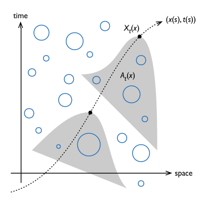
Ambit processes describe the dynamics in a stochastically developing field, for instance a turbulent wind field, along curves embedded in such a field. An illustration of the various concepts involved is demonstrated by figure 1. This shows a curve running with time through space. To each point on the curve is associated a random variable $X_{\theta}$ย which should be thought of as the value of an observation at that point. This value is assumed to depend only on a region of previous space-time, indicated by the solid line in the figure, called the ambit set associated to the point in question. Further, a key characteristic of the modelling framework, which distinguishes ambit fields from other approaches is that beyond the most basic kind of random input it also specifically incorporates additional, often drastically changing, inputs referred to as volatility or intermittency. This feature is illustrated by the blue circles whose sizes indicate volatility effects of varying degree.

In terms of mathematical formulae an ambit field is specified via

Xtโ€‹(x)=ฮผ+โˆซAtโ€‹(x)gโ€‹(t,s,x,ฮพ)โ€‹ฯƒsโ€‹(ฮพ)โ€‹Lโ€‹(dโ€‹s,dโ€‹ฮพ)+โˆซDtโ€‹(x)qโ€‹(t,s,x,ฮพ)โ€‹asโ€‹(ฮพ)โ€‹dsโ€‹dฮพsubscript๐‘‹๐‘ก๐‘ฅ๐œ‡subscriptsubscript๐ด๐‘ก๐‘ฅ๐‘”๐‘ก๐‘ ๐‘ฅ๐œ‰subscript๐œŽ๐‘ ๐œ‰๐ฟd๐‘ d๐œ‰subscriptsubscript๐ท๐‘ก๐‘ฅ๐‘ž๐‘ก๐‘ ๐‘ฅ๐œ‰subscript๐‘Ž๐‘ ๐œ‰differential-d๐‘ differential-d๐œ‰\displaystyle X_{t}(x)=\mu+\int_{A_{t}(x)}g(t,s,x,\xi)\sigma_{s}(\xi)L(\mathrm{d}s,\mathrm{d}\xi)+\int_{D_{t}(x)}q(t,s,x,\xi)a_{s}(\xi)\mathrm{d}s\mathrm{d}\xi (1.1)

where $t$ denotes time while $x$ย gives the position in space. Further, $A_{t}(x)$ and $D_{t}(x)$ are ambit sets, $g$ and $q$ are deterministic weight functions, $\sigma$ represents the volatility or intermittency field, $a$ is a drift field and $L$ denotes a Lรฉvy basis. We recall that a Lรฉvy basis $L=\{L(B):~{}B\in\mathcal{S}\}$, where $\mathcal{S}$ is a $\delta$-ring of an arbitrary non-empty set $S$ such that there exists an increasing sequence of sets $(S_{n})\subset\mathcal{S}$ with $\cup_{n\in\mathbb{N}}S_{n}=S$, is an independently scattered random measure with Lรฉvy-Khinchin representation

$\displaystyle\log\mathbb{E}[\exp(iuL(B))]=iuv_{1}(B)-\frac{1}{2}u^{2}v_{2}(B)+\int_{\mathbb{R}}\left(\exp(iuy)-1-iuy1_{[-1,1]}(y)\right)v_{3}(dy,B).$ (1.2)

Here $v_{1}$ is a signed measure on $\mathcal{S}$, $v_{2}$ is a measure on $\mathcal{S}$ and $v_{3}(\cdot,\cdot)$ is a generalised Lรฉvy measure on $\mathbb{R}\times\mathcal{S}$ (see e.g. [46] for details). In the turbulence framework the stochastic field $(X_{t}(x))_{t\geq 0,x\in\mathbb{R}^{3}}$ describes the velocity of a turbulent flow at time $t$ and position $x$, while the ambit sets $A_{t}(x),D_{t}(x)$ are typically bounded.

Triggered by the wide applicability of ambit fields there is an increasing need in understanding their mathematical properties. The main mathematical topics of interest are: stochastic analysis for ambit fields, modelling of volatility/intermittency, asymptotic theory for ambit fields, numerical approximations of ambit fields, and asymptotic statistics. The aim of this paper is to give an overview of recent studies and to point out the main challenges in future. We will see that most of the mathematical problems already arise in a null spatial setting, and therefore parts of the presented theory will deal with this case only. However, possible extensions to spatial dimension will be discussed. At this stage we would like to mention another review on ambit fields [6], which focuses on integration theory, various examples of ambit fields and their applications in physics and finance. Numerical schemes for ambit processes, which will not be demonstrated in this work, are investigated in [22].

The paper is structured as follows. We introduce the main mathematical setting and discuss some basic probabilistic properties of ambit fields in Section 2. Section 3 gives a review on integration concepts with respect to ambit fields. Section 4 is devoted to limit theorems for high frequency statistics of ambit fields and their statistical applications.

2 The model and basic probabilistic properties

Throughout this paper all stochastic processes are defined on a given probability space $(\Omega,\mathcal{F},\mathbb{P})$. We first consider a subclass of an ambit field defined via

Xtโ€‹(x)=ฮผ+โˆซA+(t,x)gโ€‹(tโˆ’s,xโˆ’ฮพ)โ€‹ฯƒsโ€‹(ฮพ)โ€‹Lโ€‹(dโ€‹sโ€‹dโ€‹ฮพ)+โˆซD+(t,x)qโ€‹(tโˆ’s,xโˆ’ฮพ)โ€‹asโ€‹(ฮพ)โ€‹dsโ€‹dฮพ,subscript๐‘‹๐‘ก๐‘ฅ๐œ‡subscript๐ด๐‘ก๐‘ฅ๐‘”๐‘ก๐‘ ๐‘ฅ๐œ‰subscript๐œŽ๐‘ ๐œ‰๐ฟd๐‘ d๐œ‰subscript๐ท๐‘ก๐‘ฅ๐‘ž๐‘ก๐‘ ๐‘ฅ๐œ‰subscript๐‘Ž๐‘ ๐œ‰differential-d๐‘ differential-d๐œ‰\displaystyle X_{t}(x)=\mu+\int_{A+(t,x)}g(t-s,x-\xi)\sigma_{s}(\xi)L(\mathrm{d}s\mathrm{d}\xi)+\int_{D+(t,x)}q(t-s,x-\xi)a_{s}(\xi)\mathrm{d}s\mathrm{d}\xi, (2.1)

where $A,D\subset\mathbb{R}\times\mathbb{R}^{d}$ are fixed ambit sets. This specific framework allows for modelling stationary random fields, namely when the field $(\sigma,a)$ is stationary and independent of the driving Lรฉvy basis $L$, $X$ turns out to be stationary too. Another potentially important features of a random field, such as e.g. isotropy or skewness, can be easily modelled via an appropriate choice of the deterministic kernels $g$ and $q$, and the stochastic field $(\sigma,a)$.

Specializing even further, we introduce a Lรฉvy semi-stationary process given by

Yt=ฮผ+โˆซโˆ’โˆžtgโ€‹(tโˆ’s)โ€‹ฯƒsโ€‹Lโ€‹(dโ€‹s)+โˆซโˆ’โˆžtqโ€‹(tโˆ’s)โ€‹asโ€‹ds,subscript๐‘Œ๐‘ก๐œ‡superscriptsubscript๐‘ก๐‘”๐‘ก๐‘ subscript๐œŽ๐‘ ๐ฟd๐‘ superscriptsubscript๐‘ก๐‘ž๐‘ก๐‘ subscript๐‘Ž๐‘ differential-d๐‘ \displaystyle Y_{t}=\mu+\int_{-\infty}^{t}g(t-s)\sigma_{s}L(\mathrm{d}s)+\int_{-\infty}^{t}q(t-s)a_{s}\mathrm{d}s, (2.2)

where now $L$ is a two-sided one dimensional Lรฉvy motion and $A=D=(-\infty,0)$, which is a purely temporal analogue of the ambit field at (2.1). It is indeed this special subclass of ambit fields, which will be the focus of our interest, as many mathematical problems have to be solved for Lรฉvy semi-stationary processes first before transferring the principles to more general random fields. In the following we will check the validity and discuss some basic properties of ambit fields. Note that we sometimes use dโ€‹Ls๐‘‘subscript๐ฟ๐‘ dL_{s} instead of Lโ€‹(dโ€‹s)๐ฟd๐‘ L(\mathrm{d}s) in the setting of (2.2). We also remark that the meaning of some notations may change from section to section.

2.1 Definition of the stochastic integral

The first natural question when introducing an ambit field is the definition of the first integral appearing in the decomposition (1.1). Here we recall two classical approaches of Rajput and Rosinski [46] and Walsh [50].

2.1.1 Rajput and Rosinski theory

The first simplified mathematical problem is the definition of stochastic integral in case of a deterministic intermittency field $\sigma$. In this situation we may study a more general integral

$$\int_{A}fdL,$$

where $L$ is a Lรฉvy basis on a $\delta$-ring $\mathcal{S}$, $f:(S,\sigma(\mathcal{S}))\rightarrow(\mathbb{R},\mathcal{B}(\mathbb{R}))$ a measurable real valued function and $A\in\sigma(\mathcal{S})$, which is the main object of a seminal paper [46]. We will briefly recall the most important results of this work. By definition of a Lรฉvy basis the law of $(L(A_{1}),\ldots,L(A_{d}))$, $A_{i}\in\mathcal{S}$, is infinitely divisible, the random variables $L(A_{1}),\ldots,L(A_{d})$ are independent when the sets $A_{1},\ldots,A_{d}$ are disjoint, and

$$L\left(\cup_{i=1}^{\infty}A_{i}\right)=\sum_{i=1}^{\infty}L(A_{i})\qquad\mathbb{P}-\text{almost surely}$$

for disjoint $A_{i}$โ€™s with $\cup_{i=1}^{\infty}A_{i}\in\mathcal{S}$. Recalling the characteristic triplet $(v_{1},v_{2},v_{3})$ from the Lรฉvy-Khinchin representation (1.2), the control measure $\lambda$ of $L$ is defined via

$$\lambda(A):=|v_{1}|(A)+v_{2}(A)+\int_{\mathbb{R}}\min(1,x^{2})v_{3}(dx,A),\qquad A\in\mathcal{S},$$

where $|v_{1}|$ denotes the total variation measure associated with $v_{1}$. In this subsection we will use the truncation function

$$\tau(z):=\left\{\begin{array}[]{cc}z:&\|z\|\leq 1\\ z/\|z\|:&\|z\|>1\end{array}\right.$$

Now, for any simple function

$$f(x)=\sum_{i=1}^{d}a_{i}1_{A_{i}}(x),\qquad a_{i}\in\mathbb{R},A_{i}\in\mathcal{S},$$

the stochastic integral is defined as

$$\int_{A}fdL:=\sum_{i=1}^{d}a_{i}L(A\cap A_{i}),\qquad A\in\sigma(\mathcal{S}).$$

The extension of this definition is as follows.

Definition 2.1

A measurable function $f:(\mathcal{S},\sigma(\mathcal{S}))\rightarrow(\mathbb{R},\mathcal{B}(\mathbb{R}))$ is called $L$-integrable if there exists a sequence of simple functions $(f_{n})_{n\geq 1}$ such that

  • (i)

    $f_{n}\rightarrow f$ $\lambda$-almost surely.

  • (ii)

    For any $A\in\sigma(\mathcal{S})$ the sequence $(\int_{A}f_{n}dL)$ converges in probability.

In this case the stochastic integral is defined by

$$\int_{A}fdL:=\mathbb{P}-\lim_{n\rightarrow\infty}\int_{A}f_{n}dL.$$

Although this definition is quite intuitive, it does not specify the class of $L$-integrable functions explicitly. The next theorem, which is one of the main results of [46], gives an explicit condition on the $L$-integrability of a function $f$.

Theorem 2.2

([46, Theorem 2.7]) Let $f:(S,\sigma(\mathcal{S}))\rightarrow(\mathbb{R},\mathcal{B}(\mathbb{R}))$ be a measurable function. Then $f$ is $L$-integrable if and only if the following conditions hold:

โˆซSUโ€‹(fโ€‹(s),s)โ€‹ฮปโ€‹(dโ€‹s)<โˆž,โˆซSf2โ€‹(s)โ€‹v2โ€‹(s)โ€‹ฮปโ€‹(dโ€‹s)<โˆž,โˆซSV0โ€‹(fโ€‹(s),s)โ€‹ฮปโ€‹(dโ€‹s)<โˆž,formulae-sequencesubscript๐‘†๐‘ˆ๐‘“๐‘ ๐‘ ๐œ†๐‘‘๐‘ formulae-sequencesubscript๐‘†superscript๐‘“2๐‘ subscript๐‘ฃ2๐‘ ๐œ†๐‘‘๐‘ subscript๐‘†subscript๐‘‰0๐‘“๐‘ ๐‘ ๐œ†๐‘‘๐‘ \int_{S}U(f(s),s)\lambda(ds)<\infty,\quad\int_{S}f^{2}(s)v_{2}(s)\lambda(ds)<\infty,\quad\int_{S}V_{0}(f(s),s)\lambda(ds)<\infty,

where

Uโ€‹(u,s)๐‘ˆ๐‘ข๐‘ \displaystyle U(u,s) :=uโ€‹v1โ€‹(s)+โˆซโ„(ฯ„โ€‹(xโ€‹u)โˆ’uโ€‹ฯ„โ€‹(x))โ€‹v3โ€‹(dโ€‹x,s),assignabsent๐‘ขsubscript๐‘ฃ1๐‘ subscriptโ„๐œ๐‘ฅ๐‘ข๐‘ข๐œ๐‘ฅsubscript๐‘ฃ3๐‘‘๐‘ฅ๐‘ \displaystyle:=uv_{1}(s)+\int_{\mathbb{R}}(\tau(xu)-u\tau(x))v_{3}(dx,s),
V0โ€‹(u,s)subscript๐‘‰0๐‘ข๐‘ \displaystyle V_{0}(u,s) :=โˆซโ„minโก(1,|xโ€‹u|2)โ€‹v3โ€‹(dโ€‹x,s).assignabsentsubscriptโ„1superscript๐‘ฅ๐‘ข2subscript๐‘ฃ3๐‘‘๐‘ฅ๐‘ \displaystyle:=\int_{\mathbb{R}}\min(1,|xu|^{2})v_{3}(dx,s).

Furthermore, the real valued random variable $X=\int_{S}fdL$ is infinitely divisible with Lรฉvy-Khinchin representation

$$\log\mathbb{E}[\exp(iuX)]=iuv_{1}(f)-\frac{1}{2}u^{2}v_{2}(f)+\int_{\mathbb{R}}\left(\exp(iuy)-1-iuy1_{[-1,1]}(y)\right)v_{3}^{f}(dy),$$

where

$\displaystyle v_{1}(f)$ =โˆซSUโ€‹(fโ€‹(s),s)โ€‹ฮปโ€‹(dโ€‹s),absentsubscript๐‘†๐‘ˆ๐‘“๐‘ ๐‘ ๐œ†๐‘‘๐‘ \displaystyle=\int_{S}U(f(s),s)\lambda(ds),
$\displaystyle v_{2}(f)$ =โˆซSf2โ€‹(s)โ€‹v2โ€‹(s)โ€‹ฮปโ€‹(dโ€‹s),absentsubscript๐‘†superscript๐‘“2๐‘ subscript๐‘ฃ2๐‘ ๐œ†๐‘‘๐‘ \displaystyle=\int_{S}f^{2}(s)v_{2}(s)\lambda(ds),
$\displaystyle v_{3}^{f}(B)$ =v3โ€‹{(x,s)โˆˆโ„ร—S:xโ€‹fโ€‹(s)โˆˆBโˆ–{0}},Bโˆˆโ„ฌโ€‹(โ„).formulae-sequenceabsentsubscript๐‘ฃ3conditional-set๐‘ฅ๐‘ โ„๐‘†๐‘ฅ๐‘“๐‘ ๐ต0๐ตโ„ฌโ„\displaystyle=v_{3}\left\{(x,s)\in\mathbb{R}\times S:~{}xf(s)\in B\setminus\{0\}\right\},\qquad B\in\mathcal{B}(\mathbb{R}).
Remark 2.3

The most basic example of a null spatial ambit field is the Lรฉvy moving average process given by

Xt=โˆซโˆ’โˆžtgโ€‹(tโˆ’s)โ€‹๐‘‘Ls,subscript๐‘‹๐‘กsuperscriptsubscript๐‘ก๐‘”๐‘ก๐‘ differential-dsubscript๐ฟ๐‘ \displaystyle X_{t}=\int_{-\infty}^{t}g(t-s)dL_{s}, (2.3)

where $L$ is a two-sided Lรฉvy motion with $\mathbb{E}L_{t}=0$. In this situation the control measure $\lambda$ is just the Lebesgue measure and the sufficient conditions from Theorem 2.2 translate to

โˆซ0โˆžg2โ€‹(s)โ€‹๐‘‘s<โˆž,โˆซ0โˆž(โˆซโ„minโก(|xโ€‹gโ€‹(s)|,|xโ€‹gโ€‹(s)|2)โ€‹v3โ€‹(dโ€‹x))โ€‹๐‘‘s<โˆž,formulae-sequencesuperscriptsubscript0superscript๐‘”2๐‘ differential-d๐‘ superscriptsubscript0subscriptโ„๐‘ฅ๐‘”๐‘ superscript๐‘ฅ๐‘”๐‘ 2subscript๐‘ฃ3๐‘‘๐‘ฅdifferential-d๐‘ \int_{0}^{\infty}g^{2}(s)ds<\infty,\quad\int_{0}^{\infty}\left(\int_{\mathbb{R}}\min(|xg(s)|,|xg(s)|^{2})v_{3}(dx)\right)ds<\infty,

where $v_{3}$ is the Lรฉvy measure of $L$. $\hfill\Box$

Theorem 2.2 gives a precise condition for existence of the stochastic integral. However, it does not say anything about the existence of moments. To study this question let us assume for the rest of this subsection that

$$\mathbb{E}[|L(A)|^{q}]<\infty\qquad\forall A\in\mathcal{S},$$

for some $q>0$. Clearly, in general we can not expect the existence of moments higher than $q$ for the integral $\int_{S}fdL$, but we may study the existence of $p$th moment with $p\leq q$. For this purpose we introduce the function $\Phi_{p}:\mathbb{R}\times S\rightarrow\mathbb{R}$ via

ฮฆpโ€‹(u,s):=Uโ‹†โ€‹(u,s)+u2โ€‹v2โ€‹(s)+Vpโ€‹(u,s),assignsubscriptฮฆ๐‘๐‘ข๐‘ superscript๐‘ˆโ‹†๐‘ข๐‘ superscript๐‘ข2subscript๐‘ฃ2๐‘ subscript๐‘‰๐‘๐‘ข๐‘ \Phi_{p}(u,s):=U^{\star}(u,s)+u^{2}v_{2}(s)+V_{p}(u,s),

where

Uโ‹†โ€‹(u,s)superscript๐‘ˆโ‹†๐‘ข๐‘ \displaystyle U^{\star}(u,s) :=supcโˆˆ[โˆ’1,1]|Uโ€‹(cโ€‹u,s)|,assignabsentsubscriptsupremum๐‘11๐‘ˆ๐‘๐‘ข๐‘ \displaystyle:=\sup_{c\in[-1,1]}|U(cu,s)|,
Vpโ€‹(u,s)subscript๐‘‰๐‘๐‘ข๐‘ \displaystyle V_{p}(u,s) :=โˆซโ„(|uโ€‹x|pโ€‹1{|uโ€‹x|>1}+|uโ€‹x|2โ€‹1{|uโ€‹x|โ‰ค1})โ€‹v3โ€‹(dโ€‹x,s),assignabsentsubscriptโ„superscript๐‘ข๐‘ฅ๐‘subscript1๐‘ข๐‘ฅ1superscript๐‘ข๐‘ฅ2subscript1๐‘ข๐‘ฅ1subscript๐‘ฃ3๐‘‘๐‘ฅ๐‘ \displaystyle:=\int_{\mathbb{R}}\left(|ux|^{p}1_{\{|ux|>1\}}+|ux|^{2}1_{\{|ux|\leq 1\}}\right)v_{3}(dx,s),

and the function $U$ is introduced in Theorem 2.2. Then

โ€–fโ€–ฮฆp:=inf{c>0:โˆซSฮฆpโ€‹(cโˆ’1โ€‹|fโ€‹(s)|,s)โ€‹ฮปโ€‹(dโ€‹s)}assignsubscriptnorm๐‘“subscriptฮฆ๐‘infimumconditional-set๐‘0subscript๐‘†subscriptฮฆ๐‘superscript๐‘1๐‘“๐‘ ๐‘ ๐œ†๐‘‘๐‘ \|f\|_{\Phi_{p}}:=\inf\left\{c>0:~{}\int_{S}\Phi_{p}(c^{-1}|f(s)|,s)\lambda(ds)\right\}

defines a norm and the vector space

๐•ƒฮฆp:={f:โˆซSฮฆpโ€‹(|fโ€‹(s)|,s)โ€‹ฮปโ€‹(dโ€‹s)<โˆž}assignsuperscript๐•ƒsubscriptฮฆ๐‘conditional-set๐‘“subscript๐‘†subscriptฮฆ๐‘๐‘“๐‘ ๐‘ ๐œ†๐‘‘๐‘ \mathbb{L}^{\Phi_{p}}:=\left\{f:~{}\int_{S}\Phi_{p}(|f(s)|,s)\lambda(ds)<\infty\right\}

equipped with $\|\cdot\|_{\Phi_{p}}$ is the so called Musielak-Orlicz space (see [46] for details). The next result gives a connection between the existence of $p$th norm of the stochastic integral and the finiteness of $\|f\|_{\Phi_{p}}$.

Theorem 2.4

([46, Theorem 3.3]) Let $p\in[0,q]$. Then it holds that

$$\mathbb{E}\left[\left|\int_{S}fdL\right|^{p}\right]<\infty\Longleftrightarrow\|f\|_{\Phi_{p}}<\infty.$$
Remark 2.5

Let $X$ be a Lรฉvy moving average process as defined at (2.3), where the driving Lรฉvy motion has characteristic triplet $(0,0,\text{const.}|x|^{-1-\beta}dx)$, i.e. $L$ is a symmetric $\beta$-stable process ($\beta\in(0,2)$) without drift. In this case the $p$th absolute moment of $X_{t}$ exists whenever $g\in L^{\beta}(\mathbb{R}_{\geq 0})$ and $p<\beta$. Moreover it holds that

$$C_{1}\mathbb{E}\left[\left|\int_{0}^{\infty}|g(x)|^{\beta}dx\right|\right]^{1/\beta}\leq\mathbb{E}[|X_{t}|^{p}]^{1/p}\leq C_{2}\mathbb{E}\left[\left|\int_{0}^{\infty}|g(x)|^{\beta}dx\right|\right]^{1/\beta}$$

for some positive constants $C_{1},C_{2}$. $\hfill\Box$

2.1.2 Walsh approach

The integration concept proposed by Walsh [50] is, in some sense, an extension of Itรดโ€™s theory to spatio-temporal setting. As in the classical Itรด calculus the martingale theory and isometry play an essential role.

Here we review the main ideas of Walsh approach. In the following we will concentrate on integration with respect to a Lรฉvy basis on bounded domains (the theory can be extended to unbounded domains in a straightforward manner, see [50]). Let $\mathcal{B}_{b}(\mathbb{R}^{d})$ the Borel $\sigma$-field generated by bounded Borel sets on $\mathbb{R}^{d}$ and $L$ a Lรฉvy basis on $[0,T]\times S$ with $S\in\mathcal{B}_{b}(\mathbb{R}^{d})$. For $S\supseteq A\in\mathcal{B}_{b}(\mathbb{R}^{d})$ we introduce the notation

$$L_{t}(A):=L((0,t]\times A).$$

Unlike in the approach of Rajput and Rosinski, which does not require any moment assumptions (which however deals only with deterministic integrands), the basic assumption of Walsh concept is:

For any $A\in\mathcal{B}_{b}(\mathbb{R}^{d})$ it holds that $\mathbb{E}[L_{t}(A)]=0$ and $L_{t}(A)\in L^{2}(\Omega,\mathcal{F},\mathbb{P})$.

Now, we introduce a right continuous filtration $(\mathcal{F}_{t})_{t\geq 0}$ via

โ„ฑt:=โˆฉฯต>0โ„ฑt+ฯต0withFt0=ฯƒโ€‹{Lsโ€‹(A):SโЇAโˆˆโ„ฌbโ€‹(โ„d),0<sโ‰คt}โˆจ๐’ฉ,formulae-sequenceassignsubscriptโ„ฑ๐‘กsubscriptitalic-ฯต0subscriptsuperscriptโ„ฑ0๐‘กitalic-ฯตwithsubscriptsuperscript๐น0๐‘ก๐œŽconditional-setsubscript๐ฟ๐‘ ๐ดformulae-sequencesuperset-of-or-equals๐‘†๐ดsubscriptโ„ฌ๐‘superscriptโ„๐‘‘0๐‘ ๐‘ก๐’ฉ\mathcal{F}_{t}:=\cap_{\epsilon>0}\mathcal{F}^{0}_{t+\epsilon}\quad\text{with}\quad F^{0}_{t}=\sigma\{L_{s}(A):~{}S\supseteq A\in\mathcal{B}_{b}(\mathbb{R}^{d}),0<s\leq t\}\vee\mathcal{N},

where $\mathcal{N}$ denotes the $\mathbb{P}$-null sets of $\mathcal{F}$. Since $L$ is a Lรฉvy basis, the stochastic field $(L_{t}(A))_{t\geq 0,S\supseteq A\in\mathcal{B}_{b}(\mathbb{R}^{d})}$ is an orthogonal martingale measure with respect to $(\mathcal{F}_{t})_{t\geq 0}$ in the sense of Walsh, i.e. $(L_{t}(A))_{t\geq 0}$ is a square integrable martingale with respect to the filtration $(\mathcal{F}_{t})_{t\geq 0}$ for any $A\in\mathcal{B}_{b}(\mathbb{R}^{d})$ and the random variables $L_{t}(A),L_{t}(B)$ are independent for disjoint sets $A,B\in\mathcal{B}_{b}(\mathbb{R}^{d})$.

In the next step we introduce the covariance measure $Q$ via

$$Q([0,t]\times A):=\langle L(A)\rangle_{t},\qquad A\in\mathcal{B}_{b}(\mathbb{R}^{d}),$$

and the associated $L^{2}$-norm

$$\|\psi\|_{Q}^{2}:=\mathbb{E}\left[\int_{[0,T]\times S}\psi^{2}(t,\xi)Q(dt,d\xi)\right]$$

for a random field $\psi$ on $[0,T]\times S$. Now, we are following the Itรดโ€™s program: We call $\psi$ an elementary random field if it has the form

ฯˆโ€‹(ฯ‰,s,ฮพ)=Xโ€‹(ฯ‰)โ€‹1(a,b]โ€‹(s)โ€‹1Aโ€‹(ฮพ),๐œ“๐œ”๐‘ ๐œ‰๐‘‹๐œ”subscript1๐‘Ž๐‘๐‘ subscript1๐ด๐œ‰\psi(\omega,s,\xi)=X(\omega)1_{(a,b]}(s)1_{A}(\xi),

where $X$ is a bounded $\mathcal{F}_{a}$-measurable random variable and $A\in\mathcal{B}_{b}(\mathbb{R}^{d})$. For such an elementary random field the integral with respect to a Lรฉvy basis is defined by ($t\leq T$)

โˆซ0tโˆซBฯˆโ€‹(s,ฮพ)โ€‹Lโ€‹(dโ€‹s,dโ€‹ฮพ):=Xโ€‹(Ltโˆงbโ€‹(AโˆฉB)โˆ’Ltโˆงaโ€‹(AโˆฉB)),Bโˆˆโ„ฌbโ€‹(โ„d),A,BโІS.formulae-sequenceassignsuperscriptsubscript0๐‘กsubscript๐ต๐œ“๐‘ ๐œ‰๐ฟ๐‘‘๐‘ ๐‘‘๐œ‰๐‘‹subscript๐ฟ๐‘ก๐‘๐ด๐ตsubscript๐ฟ๐‘ก๐‘Ž๐ด๐ตformulae-sequence๐ตsubscriptโ„ฌ๐‘superscriptโ„๐‘‘๐ด๐ต๐‘†\int_{0}^{t}\int_{B}\psi(s,\xi)L(ds,d\xi):=X(L_{t\wedge b}(A\cap B)-L_{t\wedge a}(A\cap B)),\qquad B\in\mathcal{B}_{b}(\mathbb{R}^{d}),~{}A,B\subseteq S.

By linearity this definition can be extended to the linear span given by elementary random fields. The $\sigma$-field $\mathcal{P}$ generated by elementary random fields is called predictable, and the space $\mathcal{P}_{L}=L^{2}(\Omega\times[0,T]\times S,\mathcal{P},Q)$ equipped with $\|\cdot\|_{Q}$ is a Hilbert space. Furthermore, the space of elementary functions is dense in $\mathcal{P}_{L}$. Thus, for any random field $\psi\in\mathcal{P}_{L}$, we may find a sequence of elementary random fields $\psi_{n}$ with $\|\psi_{n}-\psi\|_{Q}\rightarrow 0$ and

$$\int_{0}^{t}\int_{B}\psi(t,\xi)L(dt,d\xi):=\lim_{n\rightarrow\infty}\int_{0}^{t}\int_{B}\psi_{n}(t,\xi)L(dt,d\xi)\qquad\text{in }L^{2}(\Omega,\mathcal{F},\mathbb{P}).$$

Moreover, the Itรด type isometry

๐”ผโ€‹[|โˆซ0TโˆซSฯˆโ€‹(s,ฮพ)โ€‹Lโ€‹(dโ€‹s,dโ€‹ฮพ)|2]=โ€–ฯˆโ€–Q2๐”ผdelimited-[]superscriptsuperscriptsubscript0๐‘‡subscript๐‘†๐œ“๐‘ ๐œ‰๐ฟ๐‘‘๐‘ ๐‘‘๐œ‰2superscriptsubscriptnorm๐œ“๐‘„2\mathbb{E}\left[\left|\int_{0}^{T}\int_{S}\psi(s,\xi)L(ds,d\xi)\right|^{2}\right]=\|\psi\|_{Q}^{2}

is satisfied by construction.

Remark 2.6

The Walsh approach can be used to define ambit fields in (1.1) only when the driving Lรฉvy basis is square integrable, which excludes e.g. $\beta$-stable processes ($\beta\in(0,2)$). The recent work of [26] combines the ideas of Walsh [50] and Rajput and Rosinski [46] to propose an integration concept for random integrands and general Lรฉvy bases. It relies on an earlier work [24] by Bichteler and Jacod. A general reference for comparison of various integration concepts is [30]. $\hfill\Box$

2.2 Is an ambit field a semimartingale?

Semimartingales is nowadays a well studied object in probability theory. From theoretical perspective it is important to understand whether a given null spatial subclass of ambit fields is a semimartingale or not, since in this case one may better study its fine structure properties. Furthermore, limit theory for high frequency statistics, which will be the focus of our discussion in Section 4, has been investigated in great generality in the framework of semimartingales; we refer to [35] for a comprehensive study. Thus, new asymptotic results are only needed for ambit fields, which do not belong to the class of semimartingales.

For simplicity of exposition we concentrate on the study of Volterra type processes

Xt=โˆซโˆ’โˆžtgโ€‹(t,s)โ€‹๐‘‘Ls,subscript๐‘‹๐‘กsuperscriptsubscript๐‘ก๐‘”๐‘ก๐‘ differential-dsubscript๐ฟ๐‘ \displaystyle X_{t}=\int_{-\infty}^{t}g(t,s)dL_{s}, (2.4)

where $L$ is a Lรฉvy motion with $L_{0}=0$, which is obviously a purely temporal subclass of ambit fields. The semimartingale property can be studied with respect to the filtration generated by the driving Lรฉvy motion $L$ or with respect to the natural filtration (which is a harder task). For any $t\geq 0$, we define

$$\mathcal{F}^{L}_{t}:=\sigma(L_{s}:~{}s\leq t),\qquad\mathcal{F}^{X}_{t}:=\sigma(X_{s}:~{}s\leq t).$$

In the following we will review the main studies of the semimartingale property.

2.2.1 Semimartingale property with respect to $(\mathcal{F}^{L}_{t})$

Semimartingale property of various subclasses of Volterra type processes $X$ have been studied in the literature, see e.g. [18, 21, 38] among many others. However, in this subsection we closely follow the recent results of [19, Section 4]. We note that the original work [19] contains a study of more general processes, which are specialized in this paper to models of the form (2.4).

Let $L$ be a Lรฉvy process with characteristic triplet $(a,b^{2},\nu)$. In the following we consider stationary increments moving average model of the type

Xt=โˆซโ„[g1โ€‹(tโˆ’s)โˆ’g0โ€‹(โˆ’s)]โ€‹๐‘‘Ls,subscript๐‘‹๐‘กsubscriptโ„delimited-[]subscript๐‘”1๐‘ก๐‘ subscript๐‘”0๐‘ differential-dsubscript๐ฟ๐‘ \displaystyle X_{t}=\int_{\mathbb{R}}[g_{1}(t-s)-g_{0}(-s)]dL_{s}, (2.5)

where $g_{0},g_{1}$ are measurable functions satisfying $g_{0}(x)=g_{1}(x)=0$ for $x<0$. This obviously constitutes a subclass of (2.4). Integrability conditions can be directly extracted from Theorem 2.2. Notice that by construction the process $X$ has stationary increments, which explains the aforementioned notion. The main result of this subsection is [19, Theorem 4.2].

Theorem 2.7

Assume that the process $X$ is defined as in (2.5) and the following conditions are satisfied:

โˆซ0โˆž|g1โ€ฒโ€‹(s)|2โ€‹๐‘‘s<โˆž(whenย โ€‹b2>0),superscriptsubscript0superscriptsubscriptsuperscript๐‘”โ€ฒ1๐‘ 2differential-d๐‘ whenย superscript๐‘20\displaystyle\int_{0}^{\infty}|g^{\prime}_{1}(s)|^{2}ds<\infty\qquad(\text{when }b^{2}>0),
โˆซ0โˆžโˆซโ„minโก(|xโ€‹g1โ€ฒโ€‹(s)|,|xโ€‹g1โ€ฒโ€‹(s)|2)โ€‹ฮฝโ€‹(dโ€‹x)โ€‹๐‘‘s<โˆž.superscriptsubscript0subscriptโ„๐‘ฅsubscriptsuperscript๐‘”โ€ฒ1๐‘ superscript๐‘ฅsubscriptsuperscript๐‘”โ€ฒ1๐‘ 2๐œˆ๐‘‘๐‘ฅdifferential-d๐‘ \displaystyle\int_{0}^{\infty}\int_{\mathbb{R}}\min(|xg^{\prime}_{1}(s)|,|xg^{\prime}_{1}(s)|^{2})\nu(dx)ds<\infty.

Then $X$ is a semimartingale with respect to the filtration $(\mathcal{F}^{L}_{t})$.

Theorem 2.7 gives sufficient conditions for the semimartingale property of the process $X$. In certain special cases these conditions are also necessary as the following result from [19, Corollary 4.8] shows.

Theorem 2.8

Assume that the process $X$ is defined as in (2.5), $L$ has infinite variation on compact sets and $L_{1}$ is either square integrable or has a regular varying distribution at $\infty$ with index $\beta\in[-2,-1)$. Then $X$ is a semimartingale with respect to the filtration $(\mathcal{F}^{L}_{t})$ if and only if the following conditions are satisfied:

โˆซ0โˆž|g1โ€ฒโ€‹(s)|2โ€‹๐‘‘s<โˆž(whenย โ€‹b2>0),superscriptsubscript0superscriptsubscriptsuperscript๐‘”โ€ฒ1๐‘ 2differential-d๐‘ whenย superscript๐‘20\displaystyle\int_{0}^{\infty}|g^{\prime}_{1}(s)|^{2}ds<\infty\qquad(\text{when }b^{2}>0),
โˆซ0โˆžโˆซโ„minโก(|xโ€‹g1โ€ฒโ€‹(s)|,|xโ€‹g1โ€ฒโ€‹(s)|2)โ€‹ฮฝโ€‹(dโ€‹x)โ€‹๐‘‘s<โˆž.superscriptsubscript0subscriptโ„๐‘ฅsubscriptsuperscript๐‘”โ€ฒ1๐‘ superscript๐‘ฅsubscriptsuperscript๐‘”โ€ฒ1๐‘ 2๐œˆ๐‘‘๐‘ฅdifferential-d๐‘ \displaystyle\int_{0}^{\infty}\int_{\mathbb{R}}\min(|xg^{\prime}_{1}(s)|,|xg^{\prime}_{1}(s)|^{2})\nu(dx)ds<\infty.

In this case it has the decomposition

Xt=X0+g1โ€‹(0)โ€‹Lt+โˆซ0t(โˆซโ„g1โ€ฒโ€‹(sโˆ’u)โ€‹๐‘‘Lu)โ€‹๐‘‘s.subscript๐‘‹๐‘กsubscript๐‘‹0subscript๐‘”10subscript๐ฟ๐‘กsuperscriptsubscript0๐‘กsubscriptโ„subscriptsuperscript๐‘”โ€ฒ1๐‘ ๐‘ขdifferential-dsubscript๐ฟ๐‘ขdifferential-d๐‘ X_{t}=X_{0}+g_{1}(0)L_{t}+\int_{0}^{t}\left(\int_{\mathbb{R}}g^{\prime}_{1}(s-u)dL_{u}\right)ds.

When the driving process $L$ is a symmetric $\beta$-stable Lรฉvy motion with $\beta\in(1,2)$, i.e. the characteristic triplet is given via $(0,0,\text{const.}|x|^{-1-\beta}dx)$, the condition of Theorem 2.8 translates to

โˆซ0โˆž|g1โ€ฒโ€‹(s)|ฮฒโ€‹๐‘‘s<โˆž.superscriptsubscript0superscriptsubscriptsuperscript๐‘”โ€ฒ1๐‘ ๐›ฝdifferential-d๐‘ \int_{0}^{\infty}|g^{\prime}_{1}(s)|^{\beta}ds<\infty.
Remark 2.9

Another important subclass of stationary increments moving average models, which will be the object of investigation in Section 4, is a fractional Lรฉvy motion. A fractional Lรฉvy motion is defined as

Xt=โˆซโˆ’โˆžt[(tโˆ’s)+ฮฑโˆ’(โˆ’s)+ฮฑ]โ€‹๐‘‘Ls.subscript๐‘‹๐‘กsuperscriptsubscript๐‘กdelimited-[]subscriptsuperscript๐‘ก๐‘ ๐›ผsubscriptsuperscript๐‘ ๐›ผdifferential-dsubscript๐ฟ๐‘ \displaystyle X_{t}=\int_{-\infty}^{t}[(t-s)^{\alpha}_{+}-(-s)^{\alpha}_{+}]dL_{s}. (2.6)

When $L$ is a Brownian motion, this is one of the representation of a fractional Brownian motion with Hurst parameter $H=\alpha+1/2$ (with $\alpha\in(-1/2,1/2)$). Assume now that $\alpha>0$. Then $X$ is a semimartingale with respect to the filtration $(\mathcal{F}^{L}_{t})$ if and only if $b^{2}=0$, $\alpha\in(0,1/2)$ and

$$\int_{\mathbb{R}}|x|^{1/(1-\alpha)}\nu(dx)<\infty.$$

We refer to [19, Proposition 4.6] for details. $\hfill\Box$

Remark 2.10

Sufficient conditions for the semimartingale property for general Lรฉvy semi-stationary processes defined at (2.2) can be deduced from a seminal work [45] on Volterra type equations. $\hfill\Box$

Remark 2.11

In physical applications it may appear that an ambit field is observed along a curve in time-space. Let us consider for simplicity an ambit field of the form

Xtโ€‹(x)=โˆซAtโ€‹(x)gโ€‹(t,s,x,ฮพ)โ€‹Lโ€‹(dโ€‹s,dโ€‹ฮพ),subscript๐‘‹๐‘ก๐‘ฅsubscriptsubscript๐ด๐‘ก๐‘ฅ๐‘”๐‘ก๐‘ ๐‘ฅ๐œ‰๐ฟd๐‘ d๐œ‰X_{t}(x)=\int_{A_{t}(x)}g(t,s,x,\xi)L(\mathrm{d}s,\mathrm{d}\xi),

where $L$ is a Lรฉvy basis on $\mathbb{R}_{\geq 0}\times\mathbb{R}^{d}$. Let $\theta=(\theta_{1},\theta_{2}):[0,T]\rightarrow\mathbb{R}_{\geq 0}\times\mathbb{R}^{d}$ be a curve in time-space. Then the observed process is given by

$$Y_{t}=X_{\theta_{1}(t)}(\theta_{2}(t)).$$

The semimartingale property of the process $Y$ is still an open problem. $\hfill\Box$

2.2.2 Semimartingale property with respect to $(\mathcal{F}^{X}_{t})$

Showing the semimartingale property with respect to the natural filtration $(\mathcal{F}^{X}_{t})$ is by far a more delicate issue. In this subsection we restrict our attention to Volterra processes of the form

โˆซโ„[g1โ€‹(tโˆ’s)โˆ’g0โ€‹(โˆ’s)]โ€‹๐‘‘Ws.subscriptโ„delimited-[]subscript๐‘”1๐‘ก๐‘ subscript๐‘”0๐‘ differential-dsubscript๐‘Š๐‘ \int_{\mathbb{R}}[g_{1}(t-s)-g_{0}(-s)]dW_{s}.

where $W$ is a Brownian motion, since, to the best of our knowledge, little is known for general driving Lรฉvy processes. Here $g_{0},g_{1}$ are measurable functions satisfying the integrability condition sโ†ฆg1โ€‹(tโˆ’s)โˆ’g0โ€‹(โˆ’s)โˆˆL2โ€‹(โ„)maps-to๐‘ subscript๐‘”1๐‘ก๐‘ subscript๐‘”0๐‘ superscript๐ฟ2โ„s\mapsto g_{1}(t-s)-g_{0}(-s)\in L^{2}(\mathbb{R}) for any $t\in\mathbb{R}$ (this insures the existence of the integral). In the case $g_{0}=0$ the paper [37] provides necessary and sufficient conditions for the semimartingale property with respect to the natural filtration $(\mathcal{F}^{X}_{t})$. The work [16] extends the results to include the model defined above. The methodology of proofs is based upon Fourier transforms and Hardy functions.

We need to introduce some notation. For a function $h:\mathbb{R}\rightarrow\mathbb{R}$, $\widehat{h}:\mathbb{R}\rightarrow\mathbb{C}$ denotes its Fourier transform, i.e.

$$\widehat{h}(t):=\int_{\mathbb{R}}\exp(itx)h(x)dx.$$

For a function $f:\mathbb{R}\rightarrow S^{1}$, where $S^{1}$ denotes the unit circle on a complex plane, satisfying $\overline{f}(\cdot)=f(-\cdot)$ we define the function $\widetilde{f}:\mathbb{R}\rightarrow\mathbb{R}$ via

f~โ€‹(t):=limaโ†’โˆžโˆซโˆ’aaexpโก(iโ€‹tโ€‹s)โˆ’1[โˆ’1,1]โ€‹(s)iโ€‹sโ€‹fโ€‹(s)โ€‹๐‘‘s.assign~๐‘“๐‘กsubscriptโ†’๐‘Žsuperscriptsubscript๐‘Ž๐‘Ž๐‘–๐‘ก๐‘ subscript111๐‘ ๐‘–๐‘ ๐‘“๐‘ differential-d๐‘ \widetilde{f}(t):=\lim_{a\rightarrow\infty}\int_{-a}^{a}\frac{\exp(its)-1_{[-1,1]}(s)}{is}f(s)ds.

The main result of this subsection is [16, Theorem 3.2].

Theorem 2.12

The Gaussian process $X$ is a semimartingale with respect to the natural filtration $(\mathcal{F}^{X}_{t})$ if and only if the following conditions are satisfied:

  • (i)

    The function $g_{1}$ has the representation

    g1โ€‹(t)=b+aโ€‹f~โ€‹(t)+โˆซ0tfโ€‹h^^โ€‹(s)โ€‹๐‘‘sfor Lebesgue almost allย โ€‹tโˆˆโ„,formulae-sequencesubscript๐‘”1๐‘ก๐‘๐‘Ž~๐‘“๐‘กsuperscriptsubscript0๐‘ก^๐‘“^โ„Ž๐‘ differential-d๐‘ for Lebesgue almost allย ๐‘กโ„g_{1}(t)=b+a\widetilde{f}(t)+\int_{0}^{t}\widehat{f\hat{h}}(s)ds\qquad\text{for Lebesgue almost all }t\in\mathbb{R},

    where $a,b\in\mathbb{R}$, $f:\mathbb{R}\rightarrow S^{1}$ is a measurable function with $\overline{f}(\cdot)=f(-\cdot)$, and $h\in L^{2}(\mathbb{R})$ is 00 whenever aโ‰ 0๐‘Ž0a\not=0.

  • (ii)

    Set $\zeta=\widehat{f(\widehat{g_{1}-g_{0}})}$. When aโ‰ 0๐‘Ž0a\not=0 then

    โˆซ0r(|ฮถโ€‹(s)|โˆซsโˆžฮถ2โ€‹(u)โ€‹๐‘‘u)โ€‹๐‘‘s<โˆžโˆ€r>0,formulae-sequencesuperscriptsubscript0๐‘Ÿ๐œ๐‘ superscriptsubscript๐‘ superscript๐œ2๐‘ขdifferential-d๐‘ขdifferential-d๐‘ for-all๐‘Ÿ0\int_{0}^{r}\left(\frac{|\zeta(s)|}{\sqrt{\int_{s}^{\infty}\zeta^{2}(u)du}}\right)ds<\infty\qquad\forall r>0,

    where $0/0:=0$.

The second part of [16, Theorem 3.2] gives the canonical decomposition of $X$ in case, where the above conditions (i) and (ii) are satisfied. If $X_{0}=0$ one may choose $a,b,h$ and $f$ such that the canonical decomposition $X_{t}=M_{t}+A_{t}$ is given via

Mt=aโ€‹โˆซโ„(f~โ€‹(tโˆ’s)โˆ’f~โ€‹(โˆ’s))โ€‹๐‘‘Ws,At=โˆซ0t(โˆซโ„fโ€‹h^^โ€‹(sโˆ’u)โ€‹๐‘‘Wu)โ€‹๐‘‘s.formulae-sequencesubscript๐‘€๐‘ก๐‘Žsubscriptโ„~๐‘“๐‘ก๐‘ ~๐‘“๐‘ differential-dsubscript๐‘Š๐‘ subscript๐ด๐‘กsuperscriptsubscript0๐‘กsubscriptโ„^๐‘“^โ„Ž๐‘ ๐‘ขdifferential-dsubscript๐‘Š๐‘ขdifferential-d๐‘ M_{t}=a\int_{\mathbb{R}}(\widetilde{f}(t-s)-\widetilde{f}(-s))dW_{s},\qquad A_{t}=\int_{0}^{t}\left(\int_{\mathbb{R}}\widehat{f\hat{h}}(s-u)dW_{u}\right)ds.

In this decomposition the martingale part $M$ is a Wiener process with scaling parameter $(2\pi a)^{2}$. Finally, let us remark that in the special case $g_{1}=g_{0}$, as e.g. in the fractional Brownian motion setting, the condition (ii) of Theorem 2.12 is trivially satisfied.

2.3 Fine properties of Lรฉvy semi-stationary processes

In Section 4 we will study the limit theory for power variation of Lรฉvy semi-stationary processes

$$\sum_{i=1}^{[t/\Delta_{n}]}|Y_{i\Delta_{n}}-Y_{(i-1)\Delta_{n}}|^{p}\qquad\text{with }\Delta_{n}\rightarrow 0,$$

where the process $Y$ is defined at (2.2). A first step towards understanding the first and second order asymptotics for this class of statistics is to determine the fine scale behaviour of Lรฉvy semi-stationary processes. For simplicity of exposition we start our discussion with Lรฉvy moving average processes defined at (2.3), i.e.

Xt=โˆซโˆ’โˆžtgโ€‹(tโˆ’s)โ€‹๐‘‘Ls,subscript๐‘‹๐‘กsuperscriptsubscript๐‘ก๐‘”๐‘ก๐‘ differential-dsubscript๐ฟ๐‘ X_{t}=\int_{-\infty}^{t}g(t-s)dL_{s},

which constitute a subclass of Lรฉvy semi-stationary processes with constant intermittency and zero drift. We restrict ourselves to symmetric $\beta$-stable Lรฉvy processes $L$ with $\beta\in(0,2]$ and zero drift (thus, the Brownian motion is included).

The most interesting class of weight functions $g$ in physical applications is given via

$\displaystyle g(x)=x^{\alpha}f(x)\qquad\text{for }x>0,$ (2.7)

and $g(x)=0$ for $x\leq 0$, where $f:\mathbb{R}_{\geq 0}\rightarrow\mathbb{R}$ is a smooth function with fโ€‹(0)โ‰ 0๐‘“00f(0)\not=0 decaying fast enough at infinity to ensure the existence of the integral (see Remark 2.3). When $\beta\in(0,2)$, i.e. $L$ is a pure jump process, we further always assume that $\alpha>0$, since $\alpha<0$ leads to explosive behaviour of $X$ near jump times of $L$. Hence, for any $\beta\in(0,2]$, the Lรฉvy moving average process $X$ is continuous since $g(0)=0$ when $\beta<2$. A formal differentiation leads to the identity

$$dX_{t}=g(0+)dL_{t}+\left(\int_{-\infty}^{t}g^{\prime}(t-u)dL_{u}\right)dt.$$

According to Theorem 2.8 this identity indeed makes sense when (a) $\beta=2$, $g(0+)<\infty$ and $g^{\prime}\in L^{2}(\mathbb{R}_{\geq 0})$, or (b) $\beta\in(0,2)$ and

$$\int_{0}^{\infty}|g^{\prime}(x)|^{\beta}dx<\infty.$$

In this case the Lรฉvy moving average process $X$ is an Itรด semimartingale and the law of large numbers for its power variation is well understood (see e.g. the monograph [35]). In Section 4 we will be specifically interested in situations where $X$ is not a semimartingale. It is particularly the case under the conditions

$\displaystyle\beta=2\quad\text{and}\quad\alpha\in(-1/2,1/2)\quad\text{or}$
$\displaystyle\beta\in(0,2)\quad\text{and}\quad\alpha\in(0,1-1/\beta),$

since the above integrability condition for the function $g^{\prime}$ is not satisfied near 00. Under these conditions the derivative of the function $g$ explodes at 00. For a small $\Delta>0$, we intuitively deduce the following approximation for the increments of $X$:

$\displaystyle X_{t+\Delta}-X_{t}$ =โˆซโ„[gโ€‹(t+ฮ”โˆ’s)โˆ’gโ€‹(tโˆ’s)]โ€‹๐‘‘Lsabsentsubscriptโ„delimited-[]๐‘”๐‘กฮ”๐‘ ๐‘”๐‘ก๐‘ differential-dsubscript๐ฟ๐‘ \displaystyle=\int_{\mathbb{R}}[g(t+\Delta-s)-g(t-s)]dL_{s}
โ‰ˆโˆซt+ฮ”โˆ’ฯตt+ฮ”[gโ€‹(t+ฮ”โˆ’s)โˆ’gโ€‹(tโˆ’s)]โ€‹๐‘‘Lsabsentsuperscriptsubscript๐‘กฮ”italic-ฯต๐‘กฮ”delimited-[]๐‘”๐‘กฮ”๐‘ ๐‘”๐‘ก๐‘ differential-dsubscript๐ฟ๐‘ \displaystyle\approx\int_{t+\Delta-\epsilon}^{t+\Delta}[g(t+\Delta-s)-g(t-s)]dL_{s}
โ‰ˆfโ€‹(0)โ€‹โˆซt+ฮ”โˆ’ฯตt+ฮ”[(t+ฮ”โˆ’s)+ฮฑโˆ’(tโˆ’s)+ฮฑ]โ€‹๐‘‘Lsabsent๐‘“0superscriptsubscript๐‘กฮ”italic-ฯต๐‘กฮ”delimited-[]superscriptsubscript๐‘กฮ”๐‘ ๐›ผsuperscriptsubscript๐‘ก๐‘ ๐›ผdifferential-dsubscript๐ฟ๐‘ \displaystyle\approx f(0)\int_{t+\Delta-\epsilon}^{t+\Delta}[(t+\Delta-s)_{+}^{\alpha}-(t-s)_{+}^{\alpha}]dL_{s}
โ‰ˆfโ€‹(0)โ€‹โˆซโ„[(t+ฮ”โˆ’s)+ฮฑโˆ’(tโˆ’s)+ฮฑ]โ€‹๐‘‘Ls=X~t+ฮ”โˆ’X~t,absent๐‘“0subscriptโ„delimited-[]superscriptsubscript๐‘กฮ”๐‘ ๐›ผsuperscriptsubscript๐‘ก๐‘ ๐›ผdifferential-dsubscript๐ฟ๐‘ subscript~๐‘‹๐‘กฮ”subscript~๐‘‹๐‘ก\displaystyle\approx f(0)\int_{\mathbb{R}}[(t+\Delta-s)_{+}^{\alpha}-(t-s)_{+}^{\alpha}]dL_{s}=\widetilde{X}_{t+\Delta}-\widetilde{X}_{t},

where

X~t=fโ€‹(0)โ€‹โˆซโ„[(tโˆ’s)+ฮฑโˆ’(โˆ’s)+ฮฑ]โ€‹๐‘‘Ls,subscript~๐‘‹๐‘ก๐‘“0subscriptโ„delimited-[]superscriptsubscript๐‘ก๐‘ ๐›ผsuperscriptsubscript๐‘ ๐›ผdifferential-dsubscript๐ฟ๐‘ \displaystyle\widetilde{X}_{t}=f(0)\int_{\mathbb{R}}[(t-s)_{+}^{\alpha}-(-s)_{+}^{\alpha}]dL_{s}, (2.8)

and $\epsilon>0$ is an arbitrary small real number with $\epsilon\gg\Delta$. The formal proof of this first order approximation relies on the fact that the weight gโ€‹(t+ฮ”โˆ’s)โˆ’gโ€‹(tโˆ’s)๐‘”๐‘กฮ”๐‘ ๐‘”๐‘ก๐‘ g(t+\Delta-s)-g(t-s) attains asymptotically highest values when sโ‰ˆt๐‘ ๐‘กs\approx t, since $g^{\prime}$ explodes at 00. The stochastic process $\widetilde{X}$ is called a fractional $\beta$-stable Lรฉvy motion and its properties have been studied in several papers, see e.g. [20, 39] among others (for $\beta=2$ it is just an ordinary scaled fractional Brownian motion with Hurst parameter $H=\alpha+1/2$). In particular, $\widetilde{X}$ has stationary increments, it is $(\alpha+1/\beta)$-self similar with symmetric $\beta$-stable marginals.

The key fact to learn from this approximation is that, under above assumptions on $g$, the fine structure of a Lรฉvy moving average process $X$ with symmetric $\beta$-stable driver $L$ is similar to the fine structure of a fractional $\beta$-stable Lรฉvy motion $\widetilde{X}$. Thus, under certain conditions, one may transfer the asymptotic theory for power variation of $\widetilde{X}$ to the corresponding results for power variation of $X$. The limit theory for power variation of $\widetilde{X}$ is sometimes easier to handle than the original statistic due to stationarity of increments of $\widetilde{X}$ and their self similarity property, which allows to transform the original triangular observation scheme into a usual one when studying distributional properties (for the latter, ergodic limit theory might apply). Indeed, it is one method of proofs of laws of large numbers presented in Theorem 4.8(ii) of Section 4.

Remark 2.13

As mentioned above the fractional Lรฉvy motion defined at (2.8) is, up to a scaling factor, a fractional Brownian motion $B^{H}$ with Hurst parameter $H=\alpha+1/2\in(0,1)$ when $\beta=2$. Due to self similarity property of $B^{H}$ it is sufficient to study the asymptotic behaviour of the statistic

$$\sum_{i=1}^{[t/\Delta_{n}]}|B_{i}^{H}-B_{i-1}^{H}|^{p},\qquad p>0,$$

to investigate the limit theory for power variation of $B^{H}$. Below we review some classical results of [25, 49]. First of all, we obtain the convergence

$\displaystyle\Delta_{n}\sum_{i=1}^{[t/\Delta_{n}]}|B_{i}^{H}-B_{i-1}^{H}|^{p}\stackrel{{\scriptstyle\mbox{\tiny u.c.p.}}}{{\Longrightarrow}}m_{p}t,\qquad m_{p}:=\mathbb{E}[|\mathcal{N}(0,1)|^{p}],$ (2.9)

where $Z^{n}\stackrel{{\scriptstyle\mbox{\tiny u.c.p.}}}{{\Longrightarrow}}Z$ stands for uniform convergence in probability on compact intervals, i.e. $\sup_{t\in[0,T]}|Z^{n}_{t}-Z_{t}|\stackrel{{\scriptstyle\mathbb{P}}}{{\longrightarrow}}0$. The associated weak limit theory depends on the correlation kernel of the fractional Brownian noise and the Hermite rank of the function $h(x)=|x|^{p}-m_{p}$. Recall that the correlation kernel of the fractional Brownian noise is given via

$$\rho(j):=\text{corr}(B_{1}^{H}-B_{0}^{H},B_{j+1}^{H}-B_{j}^{H})=\frac{1}{2}\Big{(}|j+1|^{2H}-2|j|^{2H}+|j-1|^{2H}\Big{)}.$$

The Hermite expansion of the function $h$ is defined as

$$h(x)=|x|^{p}-m_{p}=\sum_{l=2}^{\infty}a_{l}H_{l}(x),$$

where $(H_{l})_{l\geq 0}$ are Hermite polynomials, i.e.

$$H_{0}=1\quad\text{and}\quad H_{l}=(-1)^{l}\exp(x^{2}/2)\frac{d}{dx^{l}}\{-\exp(x^{2}/2)\}\quad\text{for }l\geq 1.$$

The Hermite rank of $h$ is the smallest index $l$ with alโ‰ 0subscript๐‘Ž๐‘™0a_{l}\not=0, which is $2$ in our case. The condition for the validity of a central limit theorem associated with (2.9) is then

$$\sum_{j=1}^{\infty}\rho^{2}(j)<\infty,$$

where the power $2$ indicates the Hermite rank of $h$. This condition holds if and only if $H\in(0,3/4)$. For $H>3/4$ the limiting process is non-central. More precisely, the following functional limit theorems hold:

$\displaystyle 0<H<3/4$ $\displaystyle:\qquad\Delta_{n}^{-1/2}\left(\Delta_{n}\sum_{i=1}^{[t/\Delta_{n}]}|B_{i}^{H}-B_{i-1}^{H}|^{p}-m_{p}t\right)\stackrel{{\scriptstyle d}}{{\longrightarrow}}v_{p}W^{\prime}_{t},$
$\displaystyle H=3/4$ $\displaystyle:\qquad(\Delta_{n}\log{\Delta_{n}^{-1}})^{-1/2}\left(\Delta_{n}\sum_{i=1}^{[t/\Delta_{n}]}|B_{i}^{H}-B_{i-1}^{H}|^{p}-m_{p}t\right)\stackrel{{\scriptstyle d}}{{\longrightarrow}}\tilde{v}_{p}W^{\prime}_{t},$
$\displaystyle 3/4<H<1$ $\displaystyle:\qquad\Delta_{n}^{2H-2}\left(\Delta_{n}\sum_{i=1}^{[t/\Delta_{n}]}|B_{i}^{H}-B_{i-1}^{H}|^{p}-m_{p}t\right)\stackrel{{\scriptstyle d}}{{\longrightarrow}}Z_{t},$

where the weak convergence takes place on $\mathbb{D}([0,T])$ equipped with the uniform topology, $W^{\prime}$ denotes a Brownian motion and $Z$ is a Rosenblatt process (see e.g. [49]). Finally, the constants $v_{p}$ and $\tilde{v}_{p}$ are given by

$\displaystyle v_{p}$ $\displaystyle:=\sum_{l=2}^{\infty}l!a_{l}^{2}\Big{(}1+2\sum_{j=1}^{\infty}\rho^{l}(j)\Big{)},$
$\displaystyle\tilde{v}_{p}$ $\displaystyle:=2\lim_{n\rightarrow\infty}\frac{1}{\log n}\sum_{j=1}^{n-1}\frac{n-k}{n}\rho^{2}(j)\cdot\sum_{l=2}^{\infty}l!a_{l}^{2}.$

$\hfill\Box$

Remark 2.14

When $\beta\in(0,2)$ and $\alpha\in(0,1-1/\beta)$ we deduce via the $(\alpha+1/\beta)$-self similarity property and the strong ergodicity of the fractional $\beta$-stable Lรฉvy process $\widetilde{X}$

$$\Delta_{n}^{1-p(\alpha+1/\beta)}\sum_{i=1}^{[t/\Delta_{n}]}|\widetilde{X}_{i\Delta_{n}}-\widetilde{X}_{(i-1)\Delta_{n}}|^{p}\stackrel{{\scriptstyle\mbox{\tiny u.c.p.}}}{{\Longrightarrow}}c_{p}t,\qquad c_{p}:=\mathbb{E}[|\widetilde{X}_{1}-\widetilde{X}_{0}|^{p}]$$

whenever $p<\beta$. For $p>\beta$ the constant $c_{p}$ is infinite and non-ergodic limits appear, see Theorem 4.8 in Section 4. $\hfill\Box$

Remark 2.15

Once we have proved the law of large numbers for power variation of the basic process $\widetilde{X}$ as in Remarks 2.13 and 2.14 (or for the Lรฉvy moving average process $X$ defined at (2.3)), the main principles of the proof usually transfer to the integral process

It=โˆซ0tฯƒsโ€‹๐‘‘X~t,subscript๐ผ๐‘กsuperscriptsubscript0๐‘กsubscript๐œŽ๐‘ differential-dsubscript~๐‘‹๐‘กI_{t}=\int_{0}^{t}\sigma_{s}d\widetilde{X}_{t},

whenever the latter is well defined. As it was shown in e.g. [7, 29] the Bernsteinโ€™s blocking technique can be applied to deduce the law of large numbers for power variation of the process $I$. For instance, when $\widetilde{X}=B^{H}$ is a fractional Brownian motion with Hurst parameter $H$, it holds that

ฮ”n1โˆ’pโ€‹Hโ€‹โˆ‘i=1[t/ฮ”n]|Iiโ€‹ฮ”nโˆ’I(iโˆ’1)โ€‹ฮ”n|pโŸนu.c.p.mpโ€‹โˆซ0t|ฯƒs|pโ€‹๐‘‘s,superscriptโŸนu.c.p.superscriptsubscriptฮ”๐‘›1๐‘๐ปsuperscriptsubscript๐‘–1delimited-[]๐‘กsubscriptฮ”๐‘›superscriptsubscript๐ผ๐‘–subscriptฮ”๐‘›subscript๐ผ๐‘–1subscriptฮ”๐‘›๐‘subscript๐‘š๐‘superscriptsubscript0๐‘กsuperscriptsubscript๐œŽ๐‘ ๐‘differential-d๐‘ \Delta_{n}^{1-pH}\sum_{i=1}^{[t/\Delta_{n}]}|I_{i\Delta_{n}}-I_{(i-1)\Delta_{n}}|^{p}\stackrel{{\scriptstyle\mbox{\tiny u.c.p.}}}{{\Longrightarrow}}m_{p}\int_{0}^{t}|\sigma_{s}|^{p}ds,

where $\sigma$ is a stochastic process, which has finite $q$-variation with $q<1/(1-H)$ (see [29]). Quite often the same asymptotic result holds also for a subclass of ambit processes given by

Yt=โˆซโˆ’โˆžtgโ€‹(tโˆ’s)โ€‹ฯƒsโ€‹๐‘‘Ws,subscript๐‘Œ๐‘กsuperscriptsubscript๐‘ก๐‘”๐‘ก๐‘ subscript๐œŽ๐‘ differential-dsubscript๐‘Š๐‘ Y_{t}=\int_{-\infty}^{t}g(t-s)\sigma_{s}dW_{s},

where $W$ is a Brownian motion (cf. Section 4). The reason is again a similar fine structure of the processes $I$ and $Y$ (see e.g. [27, Section 2.2.3] for a detailed exposition).

Transferring a central limit theorem for the power variation of the driver $B^{H}$ to the integral process $I$ (and also in case of the process $Y$) is a more delicate issue. Apart from further assumptions on the integrand $\sigma$ a more technical and precise treatment of the Bernsteinโ€™s blocking technique is required. We refer to a recent work [28] for a detailed description of such a method, which relies on fractional calculus. $\hfill\Box$

3 Integration with respect to ambit fields

In this section we will discuss the integration concepts with respect to ambit processes of the type

Xt=โˆซ0tgโ€‹(t,s)โ€‹ฯƒsโ€‹๐‘‘Ls,subscript๐‘‹๐‘กsuperscriptsubscript0๐‘ก๐‘”๐‘ก๐‘ subscript๐œŽ๐‘ differential-dsubscript๐ฟ๐‘ X_{t}=\int_{0}^{t}g(t,s)\sigma_{s}dL_{s},

where $\sigma$ is a stochastic intermittency process and $L$ is a Lรฉvy motion. Our presentation is mainly based upon the recent work [3], where Malliavin calculus is applied to define the stochastic integral. The introduction of the integral

โˆซ0tZsโ€‹๐‘‘Xs,superscriptsubscript0๐‘กsubscript๐‘๐‘ differential-dsubscript๐‘‹๐‘ \displaystyle\int_{0}^{t}Z_{s}dX_{s}, (3.1)

for a stochastic integrand $Z$, strongly depends on whether the driving process $L$ is a Brownian motion or a pure jump Lรฉvy motion, since the main notions of Malliavin calculus differ in those two cases. An alternative way of defining the stochastic integral at (3.1) without imposing $L^{2}$-structure of the integrand $Z$ is proposed in [4]. The authors apply white noise analysis to construct the integral in the situation, where $X$ is driven by a Brownian motion.

3.1 Integration with respect to ambit processes driven by Brownian motion

Before we present the definition of the integral at (3.1) for $L=W$, we start by introducing the main notions of Malliavin calculus on Gaussian spaces. The reader is referred to the monograph [40] for any unexplained definition or result.

Let $\mathbb{H}$ be a real separable Hilbert space. We denote by $B=\{B(h):h\in\mathbb{H}\}$ an isonormal Gaussian process over $\mathbb{H}$, i.e. $B$ is a centered Gaussian family indexed by the elements of $\mathbb{H}$ and such that, for every $h_{1},h_{2}\in\mathbb{H}$,

$$\mathbb{E}\big{[}B(h_{1})B(h_{2})\big{]}=\langle h_{1},h_{2}\rangle_{\mathbb{H}}.$$ (3.2)

In what follows, we shall use the notation ${L}^{2}(B)$ $=$ $L^{2}(\Omega,\sigma(B),\mathbb{P})$. For every $q\geq 1$, we write $\mathbb{H}^{\otimes q}$ to indicate the $q$th tensor power of $\mathbb{H}$; the symbol $\mathbb{H}^{\odot q}$ indicates the $q$th symmetric tensor power of $\mathbb{H}$, equipped with the norm $\sqrt{q!}\|\cdot\|_{\mathbb{H}^{\otimes q}}$. We denote by $I_{q}$ the isometry between $\mathbb{H}^{\odot q}$ and the $q$th Wiener chaos of $X$, which is a linear map satisfying the property

$$I_{q}(h^{\otimes q}):=H_{q}(B(h)),\qquad h^{\otimes q}:=h\otimes\cdots\otimes h\in\mathbb{H}^{\otimes q}\quad\text{with }\|h\|_{\mathbb{H}}=1,$$

where $H_{q}$ is the $q$th Hermite polynomial defined in Remark 2.13. It is well-known (see [40, Chapter 1]) that any random variable $F\in L^{2}(B)$ admits an orthogonal chaotic expansion:

$$F=\sum_{q=0}^{\infty}I_{q}(f_{q}),$$ (3.3)

where $I_{0}(f_{0})=\mathbb{E}[F]$, the series converges in $L^{2}$ and the kernels $f_{q}\in\mathbb{H}^{\odot q}$, $q\geq 1$, are uniquely determined by $F$. In the particular case where $\mathbb{H}=L^{2}(A,\mathcal{A},\mu)$, with $(A,\mathcal{A})$ a measurable space and $\mu$ a $\sigma$-finite and non-atomic measure, one has that โ„โŠ™q=Ls2โ€‹(Aq,๐’œโŠ—q,ฮผโŠ—q)superscriptโ„direct-productabsent๐‘žsubscriptsuperscript๐ฟ2๐‘ superscript๐ด๐‘žsuperscript๐’œtensor-productabsent๐‘žsuperscript๐œ‡tensor-productabsent๐‘ž\mathbb{H}^{\odot q}=L^{2}_{s}(A^{q},\mathcal{A}^{\otimes q},\mu^{\otimes q}) is the space of symmetric and square integrable functions on $A^{q}$. Moreover, for every $f\in\mathbb{H}^{\odot q}$, $I_{q}(f)$ coincides with the multiple Wiener-Itรด integral (of order $q$) of $f$ with respect to $B$ (see [40, Chapter 1]).

Now, we introduce the Malliavin derivative. Let $\mathcal{S}$ be the set of all smooth cylindrical random variables of the form

$$F=f\big{(}B(h_{1}),\ldots,B(h_{n})\big{)},$$

where $n\geq 1$, $f:\mathbb{R}^{n}\rightarrow\mathbb{R}$ is a smooth function with compact support and $h_{i}\in\mathbb{H}$. The Malliavin derivative of $F$ is the element of $L^{2}(\Omega,\mathbb{H})$ defined as

$$DF:=\sum_{i=1}^{n}\frac{\partial f}{\partial x_{i}}\big{(}B(h_{1}),\ldots,B(h_{n})\big{)}h_{i}.$$

For instance, $DW(h)=h$ for every $h\in\mathbb{H}$. We denote by $\mathbb{D}^{1,2}$ the closure of $\mathcal{S}$ with respect to the norm $\|\cdot\|_{1,2}$, defined by the relation

$$\|F\|_{1,2}^{2}=\mathbb{E}[F^{2}]+\mathbb{E}[\|DF\|_{\mathbb{H}}^{2}].$$

Note that, if $F$ is equal to a finite sum of multiple Wiener-Itรด integrals, then $F\in\mathbb{D}^{1,2}$. The Malliavin derivative $D$ verifies the following chain rule: if $\varphi:\mathbb{R}^{n}\rightarrow\mathbb{R}$ is in $C^{1}_{b}$ (that is, the collection of continuously differentiable functions with bounded partial derivatives) and if $\{F_{i}\}_{i=1,\ldots,n}$ is a vector of elements of $\mathbb{D}^{1,2}$, then $\varphi(F_{1},\ldots,F_{n})\in\mathbb{D}^{1,2}$ and

$$D\varphi(F_{1},\ldots,F_{n})=\sum_{i=1}^{n}\frac{\partial\varphi}{\partial x_{i}}(F_{1},\ldots,F_{n})DF_{i}.$$

We denote by $\delta$ the adjoint of the unbounded operator $D$, also called the divergence operator. A random element $u\in L^{2}(\Omega,\mathbb{H})$ belongs to the domain of $\delta$, noted ${\rm Dom}\delta$, if and only if it verifies

$$|\mathbb{E}\langle DF,u\rangle_{\mathbb{H}}|\leq c_{u}\,\|F\|_{L^{2}}\quad\mbox{for any }F\in{\mathcal{S}},$$

where $c_{u}$ is a constant depending only on $u$. If $u\in{\rm Dom}\delta$, then the random variable $\delta(u)$ is defined by the duality relationship (sometimes called โ€˜integration by parts formulaโ€™):

$$\mathbb{E}[F\delta(u)]=\mathbb{E}\langle DF,u\rangle_{\mathbb{H}},$$ (3.4)

which holds for every $F\in\mathbb{D}^{1,2}$. An immediate consequence of (3.4) is the following identity

$\displaystyle\delta(Fu)=F\delta(u)-\langle DF,u\rangle_{\mathbb{H}},$ (3.5)

which holds for all $F\in\mathbb{D}^{1,2}$ and $u\in{\rm Dom}\delta$ such that $Fu\in{\rm Dom}\delta$.

Remark 3.1

When $\mathbb{H}=L^{2}([0,T],dx)$, which is the most basic example, then the isonormal Gaussian process $B$ is a standard Brownian motion on $[0,T]$. In this case we have

ฮดโ€‹(h)=โˆซ0Thsโ€‹๐‘‘Bs,โˆ€hโˆˆL2โ€‹([0,T],dโ€‹x).formulae-sequence๐›ฟโ„Žsuperscriptsubscript0๐‘‡subscriptโ„Ž๐‘ differential-dsubscript๐ต๐‘ for-allโ„Žsuperscript๐ฟ20๐‘‡๐‘‘๐‘ฅ\delta(h)=\int_{0}^{T}h_{s}dB_{s},\qquad\forall h\in L^{2}([0,T],dx).

The divergence operator $\delta$ is often called Skorohod integral. One can show that for a stochastic process $u\in{\rm Dom}\delta$, the Skorohod integral $\delta(u)$ and the Itรด integral โˆซ0Tusโ€‹๐‘‘Bssuperscriptsubscript0๐‘‡subscript๐‘ข๐‘ differential-dsubscript๐ต๐‘ \int_{0}^{T}u_{s}dB_{s} coincide whenever the latter is well defined.

In case $\mathbb{H}=L^{2}([0,T],dx)$ the Malliavin derivative $D$ and the divergence operator $\delta$ can be computed directly using chaos expansion. Indeed, the derivative of a random variable $F$ as in (3.3) can be identified with the element of $L^{2}([0,T]\times\Omega)$ given by

$$D_{a}F=\sum_{q=1}^{\infty}qI_{q-1}\big{(}f_{q}(\cdot,a)\big{)},\quad a\in[0,T].$$ (3.6)

On the other hand, for any $u\in L^{2}([0,T]\times\Omega)$ there exists a chaos decomposition

us=โˆ‘q=0โˆžIqโ€‹(fqโ€‹(โ‹…,s)),fqโ€‹(โ‹…,s)โˆˆLs2โ€‹([0,T]qร—ฮฉ).formulae-sequencesubscript๐‘ข๐‘ superscriptsubscript๐‘ž0subscript๐ผ๐‘žsubscript๐‘“๐‘žโ‹…๐‘ subscript๐‘“๐‘žโ‹…๐‘ subscriptsuperscript๐ฟ2๐‘ superscript0๐‘‡๐‘žฮฉu_{s}=\sum_{q=0}^{\infty}I_{q}(f_{q}(\cdot,s)),\qquad f_{q}(\cdot,s)\in L^{2}_{s}([0,T]^{q}\times\Omega).

Let f~qโˆˆLs2โ€‹([0,T]q+1ร—ฮฉ)subscript~๐‘“๐‘žsubscriptsuperscript๐ฟ2๐‘ superscript0๐‘‡๐‘ž1ฮฉ\tilde{f}_{q}\in L^{2}_{s}([0,T]^{q+1}\times\Omega) denote the symmetrization of $f_{q}(\cdot,\cdot)$. Then the element $\delta(u)$ can be written in terms of chaotic decomposition as

$$\delta(u)=\sum_{q=0}^{\infty}I_{q+1}(\tilde{f}_{q}).$$

$\hfill\Box$

Now, we start introducing the definition of the integral โˆซ0tZsโ€‹๐‘‘Xssuperscriptsubscript0๐‘กsubscript๐‘๐‘ differential-dsubscript๐‘‹๐‘ \int_{0}^{t}Z_{s}dX_{s}, where the ambit process $X$ is driven by a Brownian motion $W$. The following exposition is related to a seminal work [2], where the integration with respect to Gaussian processes has been investigated. Throughout this subsection we assume that

๐”ผโ€‹[โˆซ0tg2โ€‹(t,s)โ€‹ฯƒs2โ€‹๐‘‘s]<โˆž๐”ผdelimited-[]superscriptsubscript0๐‘กsuperscript๐‘”2๐‘ก๐‘ superscriptsubscript๐œŽ๐‘ 2differential-d๐‘ \displaystyle\mathbb{E}\left[\int_{0}^{t}g^{2}(t,s)\sigma_{s}^{2}ds\right]<\infty (3.7)

and $\mathcal{F}=\sigma(W_{t}:~{}t\in[0,T])$. The following definition is due to [3, Section 4].

Definition 3.2

Assume that, for any sโ‰ฅ0๐‘ 0s\geq 0, the function tโ†ฆgโ€‹(t,s)maps-to๐‘ก๐‘”๐‘ก๐‘ t\mapsto g(t,s) has bounded variation on the interval $[t,v]$ for all 0โ‰คs<t<v<โˆž0๐‘ ๐‘ก๐‘ฃ0\leq s<t<v<\infty. We say that the process $Z$ belongs to the class $I^{X}(0,T)$ when the following conditions are satisfied:

  • (i)

    For any sโˆˆ[0,T]๐‘ 0๐‘‡s\in[0,T] the process (Zuโˆ’Zs)uโˆˆ(s,T]subscriptsubscript๐‘๐‘ขsubscript๐‘๐‘ ๐‘ข๐‘ ๐‘‡(Z_{u}-Z_{s})_{u\in(s,T]} is integrable with respect to gโ€‹(dโ€‹u,s)๐‘”๐‘‘๐‘ข๐‘ g(du,s).

  • (ii)

    Define the operator

    ๐’ฆgโ€‹(h)โ€‹(t,s):=hโ€‹(s)โ€‹gโ€‹(t,s)+โˆซst(hโ€‹(u)โˆ’hโ€‹(s))โ€‹gโ€‹(dโ€‹u,s).assignsubscript๐’ฆ๐‘”โ„Ž๐‘ก๐‘ โ„Ž๐‘ ๐‘”๐‘ก๐‘ superscriptsubscript๐‘ ๐‘กโ„Ž๐‘ขโ„Ž๐‘ ๐‘”๐‘‘๐‘ข๐‘ \mathcal{K}_{g}(h)(t,s):=h(s)g(t,s)+\int_{s}^{t}(h(u)-h(s))g(du,s).

    The process sโ†ฆ๐’ฆgโ€‹(Z)โ€‹(T,s)โ€‹ฯƒsโ€‹1[0,T]โ€‹(s)maps-to๐‘ subscript๐’ฆ๐‘”๐‘๐‘‡๐‘ subscript๐œŽ๐‘ subscript10๐‘‡๐‘ s\mapsto\mathcal{K}_{g}(Z)(T,s)\sigma_{s}1_{[0,T]}(s) belongs to ${\rm Dom}\delta$.

  • (iii)

    ๐’ฆgโ€‹(Z)โ€‹(T,s)subscript๐’ฆ๐‘”๐‘๐‘‡๐‘ \mathcal{K}_{g}(Z)(T,s) is Malliavin differentiable with respect to Dssubscript๐ท๐‘ D_{s} with sโˆˆ[0,T]๐‘ 0๐‘‡s\in[0,T], such that the mapping sโ†ฆDsโ€‹[๐’ฆgโ€‹(Z)โ€‹(T,s)]โ€‹ฯƒsmaps-to๐‘ subscript๐ท๐‘ delimited-[]subscript๐’ฆ๐‘”๐‘๐‘‡๐‘ subscript๐œŽ๐‘ s\mapsto D_{s}[\mathcal{K}_{g}(Z)(T,s)]\sigma_{s} is Lebesgue integrable on $[0,T]$.

When $Z\in I^{X}(0,T)$ we define

โˆซ0TZsโ€‹๐‘‘Xs:=ฮดโ€‹(๐’ฆgโ€‹(Z)โ€‹(T,s)โ€‹ฯƒsโ€‹1[0,T]โ€‹(s))+โˆซ0TDsโ€‹[๐’ฆgโ€‹(Z)โ€‹(T,s)]โ€‹ฯƒsโ€‹๐‘‘s.assignsuperscriptsubscript0๐‘‡subscript๐‘๐‘ differential-dsubscript๐‘‹๐‘ ๐›ฟsubscript๐’ฆ๐‘”๐‘๐‘‡๐‘ subscript๐œŽ๐‘ subscript10๐‘‡๐‘ superscriptsubscript0๐‘‡subscript๐ท๐‘ delimited-[]subscript๐’ฆ๐‘”๐‘๐‘‡๐‘ subscript๐œŽ๐‘ differential-d๐‘ \int_{0}^{T}Z_{s}dX_{s}:=\delta\left(\mathcal{K}_{g}(Z)(T,s)\sigma_{s}1_{[0,T]}(s)\right)+\int_{0}^{T}D_{s}[\mathcal{K}_{g}(Z)(T,s)]\sigma_{s}ds.

We remark that the proposed definition is linear in the integrand. It also holds that

โˆซ0TYโ€‹Zsโ€‹๐‘‘Xs=Yโ€‹โˆซ0TZsโ€‹๐‘‘Xssuperscriptsubscript0๐‘‡๐‘Œsubscript๐‘๐‘ differential-dsubscript๐‘‹๐‘ ๐‘Œsuperscriptsubscript0๐‘‡subscript๐‘๐‘ differential-dsubscript๐‘‹๐‘ \int_{0}^{T}YZ_{s}dX_{s}=Y\int_{0}^{T}Z_{s}dX_{s}

for any bounded random variable $Y$ such that $Z,YZ\in I^{X}(0,T)$. We refer to [3] for further properties and applications.

The operator $\mathcal{K}$ has been introduced in [2]. The intuition behind Definition 3.2 is explained by the following heuristic derivation. Using classical integration by parts formula and (3.5) we conclude that

โˆซ0TZsโ€‹๐‘‘Xssuperscriptsubscript0๐‘‡subscript๐‘๐‘ differential-dsubscript๐‘‹๐‘ \displaystyle\int_{0}^{T}Z_{s}dX_{s} =ZTโ€‹XTโˆ’โˆซ0Tdโ€‹Zudโ€‹uโ€‹(โˆซ0ugโ€‹(u,s)โ€‹ฯƒsโ€‹๐‘‘Ws)โ€‹๐‘‘uabsentsubscript๐‘๐‘‡subscript๐‘‹๐‘‡superscriptsubscript0๐‘‡๐‘‘subscript๐‘๐‘ข๐‘‘๐‘ขsuperscriptsubscript0๐‘ข๐‘”๐‘ข๐‘ subscript๐œŽ๐‘ differential-dsubscript๐‘Š๐‘ differential-d๐‘ข\displaystyle=Z_{T}X_{T}-\int_{0}^{T}\frac{dZ_{u}}{du}\left(\int_{0}^{u}g(u,s)\sigma_{s}dW_{s}\right)du
=ZTโ€‹XTโˆ’โˆซ0Tฮดโ€‹(dโ€‹Zudโ€‹uโ€‹gโ€‹(u,s)โ€‹ฯƒsโ€‹1[0,T]โ€‹(s))โ€‹๐‘‘uabsentsubscript๐‘๐‘‡subscript๐‘‹๐‘‡superscriptsubscript0๐‘‡๐›ฟ๐‘‘subscript๐‘๐‘ข๐‘‘๐‘ข๐‘”๐‘ข๐‘ subscript๐œŽ๐‘ subscript10๐‘‡๐‘ differential-d๐‘ข\displaystyle=Z_{T}X_{T}-\int_{0}^{T}\delta\left(\frac{dZ_{u}}{du}g(u,s)\sigma_{s}1_{[0,T]}(s)\right)du
โˆ’โˆซ0Tโˆซ0uDsโ€‹[dโ€‹Zudโ€‹u]โ€‹gโ€‹(u,s)โ€‹ฯƒsโ€‹๐‘‘sโ€‹๐‘‘u.superscriptsubscript0๐‘‡superscriptsubscript0๐‘ขsubscript๐ท๐‘ delimited-[]๐‘‘subscript๐‘๐‘ข๐‘‘๐‘ข๐‘”๐‘ข๐‘ subscript๐œŽ๐‘ differential-d๐‘ differential-d๐‘ข\displaystyle-\int_{0}^{T}\int_{0}^{u}D_{s}\left[\frac{dZ_{u}}{du}\right]g(u,s)\sigma_{s}dsdu.

Next, the stochastic Fubini theorem applied to the last two quantities implies the identity

โˆซ0TZsโ€‹๐‘‘Xssuperscriptsubscript0๐‘‡subscript๐‘๐‘ differential-dsubscript๐‘‹๐‘ \displaystyle\int_{0}^{T}Z_{s}dX_{s} =ZTโ€‹XTโˆ’ฮดโ€‹(ฯƒsโ€‹โˆซsTgโ€‹(u,s)โ€‹dโ€‹Zudโ€‹uโ€‹๐‘‘uโ€‹1[0,T]โ€‹(s))absentsubscript๐‘๐‘‡subscript๐‘‹๐‘‡๐›ฟsubscript๐œŽ๐‘ superscriptsubscript๐‘ ๐‘‡๐‘”๐‘ข๐‘ ๐‘‘subscript๐‘๐‘ข๐‘‘๐‘ขdifferential-d๐‘ขsubscript10๐‘‡๐‘ \displaystyle=Z_{T}X_{T}-\delta\left(\sigma_{s}\int_{s}^{T}g(u,s)\frac{dZ_{u}}{du}du1_{[0,T]}(s)\right)
โˆ’โˆซ0TDsโ€‹[โˆซsTgโ€‹(u,s)โ€‹dโ€‹Zudโ€‹uโ€‹๐‘‘u]โ€‹ฯƒsโ€‹๐‘‘s.superscriptsubscript0๐‘‡subscript๐ท๐‘ delimited-[]superscriptsubscript๐‘ ๐‘‡๐‘”๐‘ข๐‘ ๐‘‘subscript๐‘๐‘ข๐‘‘๐‘ขdifferential-d๐‘ขsubscript๐œŽ๐‘ differential-d๐‘ \displaystyle-\int_{0}^{T}D_{s}\left[\int_{s}^{T}g(u,s)\frac{dZ_{u}}{du}du\right]\sigma_{s}ds.

Similarly, we deduce that

ZTโ€‹XT=ฮดโ€‹(ZTโ€‹gโ€‹(T,s)โ€‹ฯƒsโ€‹1[0,T]โ€‹(s))+โˆซ0TDsโ€‹[ZT]โ€‹gโ€‹(T,s)โ€‹ฯƒsโ€‹๐‘‘s.subscript๐‘๐‘‡subscript๐‘‹๐‘‡๐›ฟsubscript๐‘๐‘‡๐‘”๐‘‡๐‘ subscript๐œŽ๐‘ subscript10๐‘‡๐‘ superscriptsubscript0๐‘‡subscript๐ท๐‘ delimited-[]subscript๐‘๐‘‡๐‘”๐‘‡๐‘ subscript๐œŽ๐‘ differential-d๐‘ Z_{T}X_{T}=\delta\left(Z_{T}g(T,s)\sigma_{s}1_{[0,T]}(s)\right)+\int_{0}^{T}D_{s}\left[Z_{T}\right]g(T,s)\sigma_{s}ds.

Thus, putting things together and applying the classical integration by parts formula once again we obtain the heuristic formula

โˆซ0TZsโ€‹๐‘‘Xssuperscriptsubscript0๐‘‡subscript๐‘๐‘ differential-dsubscript๐‘‹๐‘ \displaystyle\int_{0}^{T}Z_{s}dX_{s} =ฮดโ€‹(ฯƒsโ€‹[ZTโ€‹gโ€‹(T,s)โˆ’โˆซsTgโ€‹(u,s)โ€‹dโ€‹Zudโ€‹uโ€‹๐‘‘u]โ€‹1[0,T]โ€‹(s))absent๐›ฟsubscript๐œŽ๐‘ delimited-[]subscript๐‘๐‘‡๐‘”๐‘‡๐‘ superscriptsubscript๐‘ ๐‘‡๐‘”๐‘ข๐‘ ๐‘‘subscript๐‘๐‘ข๐‘‘๐‘ขdifferential-d๐‘ขsubscript10๐‘‡๐‘ \displaystyle=\delta\left(\sigma_{s}\left[Z_{T}g(T,s)-\int_{s}^{T}g(u,s)\frac{dZ_{u}}{du}du\right]1_{[0,T]}(s)\right)
โˆ’โˆซ0TDsโ€‹[ZTโ€‹gโ€‹(T,s)โˆ’โˆซsTgโ€‹(u,s)โ€‹dโ€‹Zudโ€‹uโ€‹๐‘‘u]โ€‹ฯƒsโ€‹๐‘‘ssuperscriptsubscript0๐‘‡subscript๐ท๐‘ delimited-[]subscript๐‘๐‘‡๐‘”๐‘‡๐‘ superscriptsubscript๐‘ ๐‘‡๐‘”๐‘ข๐‘ ๐‘‘subscript๐‘๐‘ข๐‘‘๐‘ขdifferential-d๐‘ขsubscript๐œŽ๐‘ differential-d๐‘ \displaystyle-\int_{0}^{T}D_{s}\left[Z_{T}g(T,s)-\int_{s}^{T}g(u,s)\frac{dZ_{u}}{du}du\right]\sigma_{s}ds
=ฮดโ€‹(๐’ฆgโ€‹(Z)โ€‹(T,s)โ€‹ฯƒsโ€‹1[0,T]โ€‹(s))+โˆซ0TDsโ€‹[๐’ฆgโ€‹(Z)โ€‹(T,s)]โ€‹ฯƒsโ€‹๐‘‘s.absent๐›ฟsubscript๐’ฆ๐‘”๐‘๐‘‡๐‘ subscript๐œŽ๐‘ subscript10๐‘‡๐‘ superscriptsubscript0๐‘‡subscript๐ท๐‘ delimited-[]subscript๐’ฆ๐‘”๐‘๐‘‡๐‘ subscript๐œŽ๐‘ differential-d๐‘ \displaystyle=\delta\left(\mathcal{K}_{g}(Z)(T,s)\sigma_{s}1_{[0,T]}(s)\right)+\int_{0}^{T}D_{s}[\mathcal{K}_{g}(Z)(T,s)]\sigma_{s}ds.

This explains the intuition behind Definition 3.2.

Remark 3.3

In a recent work [23] the integration concept has been extended to the class of Hilbert-valued processes. $\hfill\Box$

3.2 Integration with respect to ambit processes driven by pure jump Lรฉvy motion

In this subsection we will introduce the definition of the integral

โˆซ0tZsโ€‹๐‘‘Xs,superscriptsubscript0๐‘กsubscript๐‘๐‘ differential-dsubscript๐‘‹๐‘ \displaystyle\int_{0}^{t}Z_{s}dX_{s},

where the ambit process $X$ is driven by a square integrable pure jump Lรฉvy motion $L$ with characteristic triplet $(0,0,\nu)$. We assume that the condition (3.7) holds and $\mathcal{F}=\sigma(L_{t}:~{}t\in[0,T])$.

The definition of the stochastic integral proposed in [3] relies again on Malliavin calculus. However, in contrast to the Gaussian space, there exist different variations of Malliavin calculus for Poisson random measures. Here we follow an approach described in [31]. We deal with the Hilbert space $\mathbb{H}=L^{2}([0,T],dx)$. Let $N(dt,dz)$ denote the Poisson random measure on $[0,T]\times(\mathbb{R}\setminus\{0\})$ associated with $L$ and $\widetilde{N}(dt,dz)=N(dt,dz)-dt\nu(dz)$ the compensated Poisson random measure. We have

$\displaystyle L_{t}=\int_{0}^{t}\int_{\mathbb{R}\setminus\{0\}}z\widetilde{N}(dt,dz).$

As in the Gaussian case there exists an orthogonal chaos decomposition of the type (3.3) in terms of multiple integrals. For any fโˆˆLs2โ€‹(([0,T]ร—(โ„โˆ–{0}))q)๐‘“subscriptsuperscript๐ฟ2๐‘ superscript0๐‘‡โ„0๐‘žf\in L^{2}_{s}(([0,T]\times(\mathbb{R}\setminus\{0\}))^{q}), we introduce the $q$th order multiple integral of $f$ with respect to $\widetilde{N}(dt,dz)$ via

$\displaystyle I_{q}(f)=q!\int_{0}^{T}\int_{\mathbb{R}\setminus\{0\}}\cdots\int_{0}^{t_{2}-}\int_{\mathbb{R}\setminus\{0\}}f(t_{1},z_{1},\ldots,t_{q},z_{q})\widetilde{N}(dt_{1},dz_{1})\ldots N(dt_{q},dz_{q}).$

Then, for any random variable $F\in L^{2}(\Omega,\mathcal{F},\mathbb{P})$, there exists a unique sequence of symmetric functions $(f_{q})_{q\geq 0}$ with fqโˆˆLs2โ€‹(([0,T]ร—(โ„โˆ–{0}))q)subscript๐‘“๐‘žsubscriptsuperscript๐ฟ2๐‘ superscript0๐‘‡โ„0๐‘žf_{q}\in L^{2}_{s}(([0,T]\times(\mathbb{R}\setminus\{0\}))^{q}) such that

$\displaystyle F=\sum_{q=0}^{\infty}I_{q}(f_{q}),$ (3.8)

which is obviously an analogue of (3.3). Furthermore, it holds that

$$\mathbb{E}[F^{2}]=\sum_{q=0}^{\infty}q!\|f_{q}\|_{q,\nu}^{2},$$

where the norm $\|f_{q}\|_{q,\nu}^{2}$ is defined by

$$\|f_{q}\|_{q,\nu}^{2}:=\int_{([0,T]\times(\mathbb{R}\setminus\{0\}))^{q}}f^{2}(t_{1},z_{1},\ldots,t_{q},z_{q})dt_{1}\nu(dz_{1})\ldots dt_{q}\nu(dz_{q}).$$

Similarly to the exposition of Remark 3.1, the Malliavin derivative $D$ and the divergence operator $\delta$ are introduced using the above chaos representation. We say that a random variable $F$ with chaos decomposition (3.8) belongs to the space $\mathbb{D}^{1,2}$ whenever the condition

$$\sum_{q=0}^{\infty}qq!\|f_{q}\|_{q,\nu}^{2}<\infty$$

holds. Whenever $F\in\mathbb{D}^{1,2}$ we define

$$D_{t,z}F:=\sum_{q=1}^{\infty}qI_{q-1}(f_{q}(\cdot,t,z)).$$

Now, we say that that a random field $u\in L^{2}([0,T]\times\mathbb{R}\setminus\{0\}\times\Omega)$ belongs to the domain of the divergence operator $\delta$ (${\rm Dom}\delta$) when

$$\left|\mathbb{E}\left[\int_{0}^{T}\int_{\mathbb{R}\setminus\{0\}}u(t,z)D_{t,z}F\nu(dz)dt\right]\right|\leq c_{u}\|F\|_{L^{2}}$$

for all $F\in\mathbb{D}^{1,2}$. Whenever $u\in{\rm Dom}\delta$ the element $\delta(u)$ is uniquely characterized via the identity

$$\mathbb{E}[F\delta(u)]=\mathbb{E}\left[\int_{0}^{T}\int_{\mathbb{R}\setminus\{0\}}u(t,z)D_{t,z}F\nu(dz)dt\right]\qquad\forall F\in\mathbb{D}^{1,2},$$

which is an integration by parts formula (cf. (3.4)). An immediate consequence of the integration by parts formula is the following equation:

$\displaystyle F\delta(u)=\delta(u(F+DF))+\int_{0}^{T}\int_{\mathbb{R}\setminus\{0\}}u(t,z)D_{t,z}F\nu(dz)dt,$ (3.9)

which holds for any $F\in\mathbb{D}^{1,2}$, $u\in{\rm Dom}\delta$ such that $u(F+DF)\in{\rm Dom}\delta$. Notice the appearance of the term $uDF$ on the right hand side that is absent in the Gaussian case (cf. (3.5)).

Now, we proceed with the introduction of the stochastic integral. Its definition in the pure jump Lรฉvy framework is essentially analogous to the Gaussian case. We refer again to [3, Section 4] for a more detailed exposition and the intuition behind this definition.

Definition 3.4

Assume that, for any sโ‰ฅ0๐‘ 0s\geq 0, the function tโ†ฆgโ€‹(t,s)maps-to๐‘ก๐‘”๐‘ก๐‘ t\mapsto g(t,s) has bounded variation on the interval $[t,T]$. We say that the process $Z$ belongs to the class $I^{X}(0,T)$ when the following conditions are satisfied:

  • (i)

    For any sโˆˆ[0,T]๐‘ 0๐‘‡s\in[0,T] the process (Zuโˆ’Zs)uโˆˆ(s,T]subscriptsubscript๐‘๐‘ขsubscript๐‘๐‘ ๐‘ข๐‘ ๐‘‡(Z_{u}-Z_{s})_{u\in(s,T]} is integrable with respect to gโ€‹(dโ€‹u,s)๐‘”๐‘‘๐‘ข๐‘ g(du,s).

  • (ii)

    The process (s,z)โ†ฆzโ€‹(๐’ฆgโ€‹(Z)โ€‹(T,s)+Ds,zโ€‹[๐’ฆgโ€‹(Z)โ€‹(T,s)])โ€‹ฯƒsโ€‹1[0,T]โ€‹(s)maps-to๐‘ ๐‘ง๐‘งsubscript๐’ฆ๐‘”๐‘๐‘‡๐‘ subscript๐ท๐‘ ๐‘งdelimited-[]subscript๐’ฆ๐‘”๐‘๐‘‡๐‘ subscript๐œŽ๐‘ subscript10๐‘‡๐‘ (s,z)\mapsto z(\mathcal{K}_{g}(Z)(T,s)+D_{s,z}[\mathcal{K}_{g}(Z)(T,s)])\sigma_{s}1_{[0,T]}(s) belongs to ${\rm Dom}\delta$.

  • (iii)

    ๐’ฆgโ€‹(Z)โ€‹(T,s)subscript๐’ฆ๐‘”๐‘๐‘‡๐‘ \mathcal{K}_{g}(Z)(T,s) is Malliavin differentiable with respect to Ds,zsubscript๐ท๐‘ ๐‘งD_{s,z} with (s,z)โˆˆ[0,T]ร—โ„๐‘ ๐‘ง0๐‘‡โ„(s,z)\in[0,T]\times\mathbb{R}, such that the mapping (s,z)โ†ฆzโ€‹Ds,zโ€‹[๐’ฆgโ€‹(Z)โ€‹(T,s)]โ€‹ฯƒsmaps-to๐‘ ๐‘ง๐‘งsubscript๐ท๐‘ ๐‘งdelimited-[]subscript๐’ฆ๐‘”๐‘๐‘‡๐‘ subscript๐œŽ๐‘ (s,z)\mapsto zD_{s,z}[\mathcal{K}_{g}(Z)(T,s)]\sigma_{s} is $\nu(dz)dt$-integrable.

When $Z\in I^{X}(0,T)$ we define

โˆซ0TZsโ€‹๐‘‘Xssuperscriptsubscript0๐‘‡subscript๐‘๐‘ differential-dsubscript๐‘‹๐‘ \displaystyle\int_{0}^{T}Z_{s}dX_{s} :=ฮดโ€‹(zโ€‹(๐’ฆgโ€‹(Z)โ€‹(T,s)+Ds,zโ€‹[๐’ฆgโ€‹(Z)โ€‹(T,s)])โ€‹ฯƒsโ€‹1[0,T]โ€‹(s))assignabsent๐›ฟ๐‘งsubscript๐’ฆ๐‘”๐‘๐‘‡๐‘ subscript๐ท๐‘ ๐‘งdelimited-[]subscript๐’ฆ๐‘”๐‘๐‘‡๐‘ subscript๐œŽ๐‘ subscript10๐‘‡๐‘ \displaystyle:=\delta\left(z(\mathcal{K}_{g}(Z)(T,s)+D_{s,z}[\mathcal{K}_{g}(Z)(T,s)])\sigma_{s}1_{[0,T]}(s)\right)
+โˆซ0Tโˆซโ„zโ€‹Ds,zโ€‹[๐’ฆgโ€‹(Z)โ€‹(T,s)]โ€‹ฯƒsโ€‹ฮฝโ€‹(dโ€‹z)โ€‹๐‘‘s.superscriptsubscript0๐‘‡subscriptโ„๐‘งsubscript๐ท๐‘ ๐‘งdelimited-[]subscript๐’ฆ๐‘”๐‘๐‘‡๐‘ subscript๐œŽ๐‘ ๐œˆ๐‘‘๐‘งdifferential-d๐‘ \displaystyle+\int_{0}^{T}\int_{\mathbb{R}}zD_{s,z}[\mathcal{K}_{g}(Z)(T,s)]\sigma_{s}\nu(dz)ds.

4 Limit theory for high frequency observations of ambit fields

In this section we will review the asymptotic results for power variation of Lรฉvy semi-stationary processes (LSS) without drift, i.e.

Yt=ฮผ+โˆซโˆ’โˆžtgโ€‹(tโˆ’s)โ€‹ฯƒsโ€‹Lโ€‹(dโ€‹s).subscript๐‘Œ๐‘ก๐œ‡superscriptsubscript๐‘ก๐‘”๐‘ก๐‘ subscript๐œŽ๐‘ ๐ฟd๐‘ Y_{t}=\mu+\int_{-\infty}^{t}g(t-s)\sigma_{s}L(\mathrm{d}s).

We will see that the limit theory heavily depends on whether the driving Lรฉvy motion is a Brownian motion or a pure jump process. Furthermore, the structure of the weight function $g$ plays an important role as we will see below. More precisely, the singularity points of $g$ determine the type of the limit.

In what follows we assume that the underlying observations of Lรฉvy semi-stationary process $Y$ are

$$Y_{0},Y_{\Delta_{n}},Y_{2\Delta_{n}},\ldots,Y_{\Delta_{n}[t/\Delta_{n}]}$$

with $\Delta_{n}\rightarrow 0$ and $t$ fixed. In other words, we are in the infill asymptotics setting. For statistical purposes we introduce $k$th order differences $\Delta_{i,k}^{n}Y$ of $Y$ defined via

$\displaystyle\Delta_{i,k}^{n}Y:=\sum_{j=0}^{k}(-1)^{j}\binom{k}{j}Y_{(i-j)\Delta_{n}}.$ (4.1)

For instance,

$$\Delta_{i,1}^{n}Y=Y_{i\Delta_{n}}-Y_{(i-1)\Delta_{n}}\quad\textrm{and}\quad\Delta_{i,2}^{n}Y=Y_{i\Delta_{n}}-2Y_{(i-1)\Delta_{n}}+Y_{(i-2)\Delta_{n}}.$$

The power variation of $k$th order differences of $Y$ is given by the statistic

$\displaystyle V(Y,p,k;\Delta_{n})_{t}$ $\displaystyle:=\sum_{i=k}^{[t/\Delta_{n}]}|\Delta_{i,k}^{n}Y|^{p}.$ (4.2)

In the following we will study the asymptotic behaviour of the functional $V(Y,p,k;\Delta_{n})_{t}$.

4.1 LSS processes driven by Brownian motion

In this section we consider the case of Brownian semi-stationary processes given via

Yt=ฮผ+โˆซโˆ’โˆžtgโ€‹(tโˆ’s)โ€‹ฯƒsโ€‹Wโ€‹(dโ€‹s),subscript๐‘Œ๐‘ก๐œ‡superscriptsubscript๐‘ก๐‘”๐‘ก๐‘ subscript๐œŽ๐‘ ๐‘Šd๐‘ Y_{t}=\mu+\int_{-\infty}^{t}g(t-s)\sigma_{s}W(\mathrm{d}s),

defined on a filtered probability space $(\Omega,\mathcal{F},(\mathcal{F}_{t})_{t\in\mathbb{R}},\mathbb{P})$. The following asymptotic results have been investigated in a series of papers [8, 9, 27, 32]. We also refer to a related work [7, 29], where the power variation of integral processes as defined in Remark 2.15 has been studied.

In the model introduced above $W$ is an $(\mathcal{F}_{t})_{t\in\mathbb{R}}$-adapted white noise on $\mathbb{R}$, $g:\mathbb{R}\rightarrow\mathbb{R}$ is a deterministic weight function satisfying $g(t)=0$ for $t\leq 0$ and $g\in\mathbb{L}^{2}(\mathbb{R})$. The intermittency process $\sigma$ is assumed to be an ย (โ„ฑt)tโˆˆโ„subscriptsubscriptโ„ฑ๐‘ก๐‘กโ„(\mathcal{F}_{t})_{t\in\mathbb{R}}-adapted cร dlร g process. The finiteness of the process $X$ is guaranteed by the condition

โˆซโˆ’โˆžtg2โ€‹(tโˆ’s)โ€‹ฯƒs2โ€‹๐‘‘s<โˆžalmost surely,superscriptsubscript๐‘กsuperscript๐‘”2๐‘ก๐‘ subscriptsuperscript๐œŽ2๐‘ differential-d๐‘ almost surely\displaystyle\int_{-\infty}^{t}g^{2}(t-s)\sigma^{2}_{s}ds<\infty\quad\text{almost surely}, (4.3)

for any $t\in\mathbb{R}$, which we assume from now on. As pointed out in [8, 9] and also briefly discussed in Remark 2.15, the Gaussian core $G$ is crucial for understanding the fine structure of $Y$. The process $G=(G_{t})_{t\in\mathbb{R}}$ is a zero-mean stationary Gaussian process given by

Gt:=โˆซโˆ’โˆžtgโ€‹(tโˆ’s)โ€‹Wโ€‹(dโ€‹s),tโˆˆโ„.formulae-sequenceassignsubscript๐บ๐‘กsuperscriptsubscript๐‘ก๐‘”๐‘ก๐‘ ๐‘Š๐‘‘๐‘ ๐‘กโ„\displaystyle G_{t}:=\int_{-\infty}^{t}g(t-s)W(ds),\qquad t\in\mathbb{R}. (4.4)

We remark that $G_{t}<\infty$ since $g\in\mathbb{L}^{2}(\mathbb{R})$. A straightforward computation shows that the correlation kernel $r$ of $G$ has the form

$$r(t)=\frac{\int_{0}^{\infty}g(u)g(u+t)du}{\|g\|_{\mathbb{L}^{2}(\mathbb{R})}^{2}},\qquad t\geq 0.$$

Another important quantity for the asymptotic theory is the variogram $R$, i.e.

Rโ€‹(t):=๐”ผโ€‹[(Gt+sโˆ’Gs)2]=2โ€‹โ€–gโ€–๐•ƒ2โ€‹(โ„)2โ€‹(1โˆ’rโ€‹(t)),ฯ„kโ€‹(ฮ”n):=๐”ผโ€‹[(ฮ”i,knโ€‹G)2].formulae-sequenceassign๐‘…๐‘ก๐”ผdelimited-[]superscriptsubscript๐บ๐‘ก๐‘ subscript๐บ๐‘ 22superscriptsubscriptnorm๐‘”superscript๐•ƒ2โ„21๐‘Ÿ๐‘กassignsubscript๐œ๐‘˜subscriptฮ”๐‘›๐”ผdelimited-[]superscriptsuperscriptsubscriptฮ”๐‘–๐‘˜๐‘›๐บ2\displaystyle R(t):=\mathbb{E}[(G_{t+s}-G_{s})^{2}]=2\|g\|_{\mathbb{L}^{2}(\mathbb{R})}^{2}(1-r(t)),\qquad\tau_{k}(\Delta_{n}):=\sqrt{\mathbb{E}[(\Delta_{i,k}^{n}G)^{2}]}. (4.5)

The quantity $\tau_{k}(\Delta_{n})$ will appear as a proper scaling in the law of large numbers for the statistic $V(Y,p,k;\Delta_{n})$ introduced at (4.2).

As mentioned above the set of singularity points $0=\theta_{0}<\theta_{1}<\cdots<\theta_{l}<\infty$ of $g$ will determine the limit theory for the power variation $V(Y,p,k;\Delta_{n})$. Let $\alpha_{0},\ldots,\alpha_{l}\in(-1/2,0)\cup(0,1/2)$ be given real numbers. For any function $h\in C^{m}(\mathbb{R})$, $h^{(m)}$ denotes the $m$-th derivative of $h$. Recall that $k\geq 1$ stands for the order of the filter defined in (4.1). We introduce the following set of assumptions.

(A): For $\delta<\frac{1}{2}\min_{1\leq i\leq l}(\theta_{i}-\theta_{i-1})$ it holds that

(i) $g(x)=x^{\alpha_{0}}f_{0}(x)$ for $x\in(0,\delta)$ and $g(x)=|x-\theta_{l}|^{\alpha_{l}}f_{l}(x)$ for $x\in(\theta_{l}-\delta,\theta_{l})\cup(\theta_{l},\infty)$.

(ii) $g(x)=|x-\theta_{i}|^{\alpha_{i}}f_{i}(x)$ for $x\in(\theta_{i}-\delta,\theta_{i})\cup(\theta_{i},\theta_{i}+\delta)$, $i=1,\ldots,l-1$.

(iii) $g(\theta_{i})=0$, $f_{i}\in C^{k}\left((\theta_{i}-\delta,\theta_{i}+\delta)\right)$ and fiโ€‹(ฮธi)โ‰ 0subscript๐‘“๐‘–subscript๐œƒ๐‘–0f_{i}(\theta_{i})\not=0 for $i=0,\ldots,l$.

(iv) $g\in C^{k}(\mathbb{R}\setminus\{\theta_{0},\ldots,\theta_{l}\})$ and $g^{(k)}\in\mathbb{L}^{2}\left(\mathbb{R}\setminus\cup_{i=0}^{l}(\theta_{i}-\delta,\theta_{i}+\delta)\right)$.

(v) For any $t>0$

Ft=โˆซฮธl+1โˆžg(k)โ€‹(s)2โ€‹ฯƒtโˆ’s2โ€‹๐‘‘s<โˆž.subscript๐น๐‘กsuperscriptsubscriptsubscript๐œƒ๐‘™1superscript๐‘”๐‘˜superscript๐‘ 2superscriptsubscript๐œŽ๐‘ก๐‘ 2differential-d๐‘ \displaystyle F_{t}=\int_{\theta_{l}+1}^{\infty}g^{(k)}(s)^{2}\sigma_{t-s}^{2}ds<\infty. (4.6)

We also set

$\displaystyle\alpha:=\min\{\alpha_{0},\ldots,\alpha_{l}\},\qquad\mathcal{A}:=\{0\leq i\leq l:~{}\alpha_{i}=\alpha\}.$ (4.7)

The points $\theta_{0},\ldots,\theta_{l}$ are singularities of $g$ in the sense that $g^{(k)}$ is not square integrable around these points, because $\alpha_{0},\ldots,\alpha_{l}\in(-1/2,0)\cup(0,1/2)$ and conditions (A)(i)-(iii) hold. Condition (A)(iv) indicates that $g$ exhibits no further singularities.

Remark 4.1

According to the discussion of Section 2.3, the Brownian semi-stationary processes $Y$ (or even the Gaussian core $G$) is not a semimartingale, since $g^{\prime}\not\in L^{2}(\mathbb{R}_{\geq 0})$ due to the presence of the singularity points $\theta_{0},\ldots,\theta_{l}$. For this reason we can not rely on limit theory for power variations of continuous semimartingales investigated in e.g. [11, 34]. Although some of the asymptotic results look similar to the semimartingale case, the methodology behind the proof is completely different. The main steps of the proof are based on methods of Malliavin calculus developed in e.g. [41, 44] and on Bernsteinโ€™s blocking technique. $\hfill\Box$

The limit theory for the power variation is quite different according to whether we have a single singularity at, say, $\theta_{0}=0$ (i.e. $l=0$) or multiple singularity points. Hence, we will treat the corresponding results separately.

4.1.1 The case $l=0$

The theory presented in this section is mainly investigated in [8, 9]. Below we will intensively use the concept of stable convergence, which is originally due to Rรฉnyi [47]. We say that a sequence of processes $X^{n}$ converges stably in law to a process $X$, where $X$ is defined on an extension $(\Omega^{\prime},\mathcal{F}^{\prime},\mathbb{P}^{\prime})$ of the original probability $(\Omega,\mathcal{F},\mathbb{P})$, in the space $\mathbb{D}([0,T])$ equipped with the uniform topology (XnโŸถdsโ€‹tXsuperscriptโŸถsubscript๐‘‘๐‘ ๐‘กsuperscript๐‘‹๐‘›๐‘‹X^{n}\stackrel{{\scriptstyle d_{st}}}{{\longrightarrow}}X) if and only if

$$\lim_{n\rightarrow\infty}\mathbb{E}[f(X^{n})Z]=\mathbb{E}^{\prime}[f(X)Z]$$

for any bounded and continuous function $f:\mathbb{D}([0,T])\rightarrow\mathbb{R}$ and any bounded $\mathcal{F}$-measurable random variable $Z$. We refer to [1], [36] or [47] for a detailed study of stable convergence. Note that stable convergence is a stronger mode of convergence than weak convergence, but it is weaker that u.c.p. convergence.

The following theorem has been shown in [9, Theorems 1 and 2].

Theorem 4.2

Assume that condition (A) holds.

  • (i)

    We obtain that

    ฮ”nโ€‹ฯ„kโ€‹(ฮ”n)โˆ’pโ€‹Vโ€‹(Y,p,k;ฮ”n)tโŸนu.c.p.Vโ€‹(Y,p)t:=mpโ€‹โˆซ0t|ฯƒs|pโ€‹๐‘‘s,superscriptโŸนu.c.p.subscriptฮ”๐‘›subscript๐œ๐‘˜superscriptsubscriptฮ”๐‘›๐‘๐‘‰subscript๐‘Œ๐‘๐‘˜subscriptฮ”๐‘›๐‘ก๐‘‰subscript๐‘Œ๐‘๐‘กassignsubscript๐‘š๐‘superscriptsubscript0๐‘กsuperscriptsubscript๐œŽ๐‘ ๐‘differential-d๐‘ \displaystyle\Delta_{n}\tau_{k}(\Delta_{n})^{-p}V(Y,p,k;\Delta_{n})_{t}\stackrel{{\scriptstyle\mbox{\tiny u.c.p.}}}{{\Longrightarrow}}V(Y,p)_{t}:=m_{p}\int_{0}^{t}|\sigma_{s}|^{p}ds, (4.8)

    where the power variation $V(Y,p,k;\Delta_{n})_{t}$ is defined at (4.2) and the constant $m_{p}$ is given by (2.9).

  • (ii)

    Assume that the intermittency process $\sigma$ is Hรถlder continuous of order $\gamma\in(0,1)$ and $\gamma(p\wedge 1)>1/2$. When $k=1$ we further assume that $\alpha\in(-1/2,0)$. Then we obtain the stable convergence

    ฮ”nโˆ’1/2โ€‹(ฮ”nโ€‹ฯ„kโ€‹(ฮ”n)โˆ’pโ€‹Vโ€‹(Y,p,k;ฮ”n)tโˆ’Vโ€‹(Y,p)t)โŸถdsโ€‹tฮปโ€‹โˆซ0t|ฯƒs|pโ€‹๐‘‘BssuperscriptโŸถsubscript๐‘‘๐‘ ๐‘กsuperscriptsubscriptฮ”๐‘›12subscriptฮ”๐‘›subscript๐œ๐‘˜superscriptsubscriptฮ”๐‘›๐‘๐‘‰subscript๐‘Œ๐‘๐‘˜subscriptฮ”๐‘›๐‘ก๐‘‰subscript๐‘Œ๐‘๐‘ก๐œ†superscriptsubscript0๐‘กsuperscriptsubscript๐œŽ๐‘ ๐‘differential-dsubscript๐ต๐‘ \displaystyle\Delta_{n}^{-1/2}\Big{(}\Delta_{n}\tau_{k}(\Delta_{n})^{-p}V(Y,p,k;\Delta_{n})_{t}-V(Y,p)_{t}\Big{)}\stackrel{{\scriptstyle d_{st}}}{{\longrightarrow}}\lambda\int_{0}^{t}|\sigma_{s}|^{p}~{}dB_{s} (4.9)

    on $\mathbb{D}([0,T])$ equipped with the uniform topology, where $B$ is a Brownian motion that is defined on an extension of the original probability space $(\Omega,\mathcal{F},\mathbb{P})$ and is independent of $\mathcal{F}$, and the constant $\lambda$ is given by

    $\displaystyle\lambda^{2}=\lim_{n\rightarrow\infty}\Delta_{n}^{-1}\mathrm{var}\Big{(}\Delta_{n}^{1-pH}V(B^{H},p,k;\Delta_{n})_{1}\Big{)},\qquad$ (4.10)

    with $B^{H}$ being a fractional Brownian motion with Hurst parameter $H=\alpha+1/2$.

Remark 4.3

The appearance of the fractional Brownian motion in the definition of the constant $\lambda^{2}$ is not surprising given the discussion of fine properties of the Gaussian core $G$ in Section 2.3. In case $k=1$ the factor $\lambda^{2}$ coincides with the quantity $v_{p}$ defined in Remark 2.13. We also remark that the validity region of the central limit theorem in (4.9) in the case $k=1$ ($\alpha\in(-1/2,0)$) is smaller than the region $H=\alpha+1/2\in(0,3/4)$ described in Remark 2.13. This is due to a bias problem, which appears in the context of Brownian semi-stationary processes. $\hfill\Box$

Notice that the asymptotic result at (4.8) and (4.9) are not feasible from the statistical point of view, since the scaling $\tau_{k}(\Delta_{n})$ depends on the unknown weight function $g$. Nevertheless, Theorem 4.2 is useful for statistical applications. Our first example is the estimation of the smoothness parameter $\alpha$. Under mild conditions on the intermittency process $\sigma$, the Brownian semi-stationary process $Y$ (as well as its Gaussian core $G$) has Hรถlder continuous paths of any order smaller than $H=\alpha+1/2\in(0,1)$. In turbulence the smoothness parameter $\alpha$ is related to the so called Kolmogorovโ€™s $2/3$-law, which predicts that

$$\mathbb{E}[(X_{t+\Delta}-X_{t})^{2}]\propto\Delta^{2/3},$$

or in other words $\alpha\approx-1/6$, which holds for a certain range of frequencies $\Delta$. Hence, estimation of the parameter $\alpha$ is extremely important.

A typical model for the weight function $g$ is the Gamma kernel given via

$$g(x)=x^{\alpha}\exp(-cx),\qquad c>0,\alpha\in(-1/2,0)\cup(0,1/2),$$

which obviously satisfies the assumption (A)(i)-(iv) with $l=0$. An application of the law of large numbers at (4.8) for a fixed $t>0$ gives

$\displaystyle S_{n}:=\frac{V(Y,p,k;2\Delta_{n})_{t}}{V(Y,p,k;\Delta_{n})_{t}}\stackrel{{\scriptstyle\mathbb{P}}}{{\longrightarrow}}2^{\frac{(2\alpha+1)p}{2}},$

since $\tau_{k}(2\Delta_{n})^{2}/\tau_{k}(\Delta_{n})^{2}\rightarrow 2^{2\alpha+1}$. The latter is due to $\tau_{k}(\Delta_{n})^{2}\sim\Delta_{n}^{2\alpha+1}$, which follows from the fact that the Gaussian core $G$ and the fractional Brownian motion $B^{H}$ with Hurst parameter $H=\alpha+1/2$ have the same small scale behaviour. Thus, a consistent estimator of $\alpha$ is given via

$\displaystyle\widehat{\alpha}_{n}=\frac{1}{2}\left(\frac{2\log_{2}S_{n}}{p}-1\right)\stackrel{{\scriptstyle\mathbb{P}}}{{\longrightarrow}}\alpha,$ (4.11)

where $\log_{2}$ denotes the logarithm at basis $2$. Note that the estimator $\widehat{\alpha}_{n}$ is feasible, i.e. it does not depend on the unknown scaling $\tau_{k}(\Delta_{n})$. One may also deduce a standard feasible central limit theorem for $\widehat{\alpha}_{n}$ as it was shown in [8, 9, 27], and thus obtain asymptotic confidence regions for the smoothness parameter $\alpha$. We also refer to [27] for empirical implementation of this estimation method to turbulence data.

Another useful application of Theorem 4.2 is the estimation of the relative intermittency, which is defined as

Rโ€‹It:=โˆซ0tฯƒs2โ€‹๐‘‘sโˆซ0Tฯƒs2โ€‹๐‘‘s,tโ‰คT,formulae-sequenceassign๐‘…subscript๐ผ๐‘กsuperscriptsubscript0๐‘กsuperscriptsubscript๐œŽ๐‘ 2differential-d๐‘ superscriptsubscript0๐‘‡superscriptsubscript๐œŽ๐‘ 2differential-d๐‘ ๐‘ก๐‘‡RI_{t}:=\frac{\int_{0}^{t}\sigma_{s}^{2}ds}{\int_{0}^{T}\sigma_{s}^{2}ds},\qquad t\leq T,

where $T>0$ is a fixed time. While the intermittency process $\sigma$ is not identifiable when no structural assumption on $g$ are imposed, the relative intermittency $RI_{t}$ is easy to estimate. Indeed, the convergence in (4.8) immediately implies that

$$\widehat{RI}_{t}^{n}:=\frac{V(Y,p,k;\Delta_{n})_{t}}{V(Y,p,k;\Delta_{n})_{T}}\stackrel{{\scriptstyle\mathbb{P}}}{{\longrightarrow}}RI_{t}.$$

We refer to [12] for the limit theory and physical applications of the statistic $\widehat{RI}_{t}^{n}$.

4.1.2 The case $l\geq 1$

The limit theory for the case $l\geq 1$ appears to be more complex. The asymptotic results presented below have been investigated in [32].

First of all, we need to introduce some notations. Recall that $k\in\mathbb{N}$ denotes the order of increments. The $k$-th order filter associated with $g$ is introduced via

$\displaystyle\Delta_{k}^{n}g(x):=\sum_{j=0}^{k}(-1)^{j}\binom{k}{j}g(x-j\Delta_{n}),\qquad x\in\mathbb{R}.$ (4.12)

There is a straightforward relationship between the scaling quantity $\tau_{k}(\Delta_{n})$ defined at (4.5) and the function $\Delta_{k}^{n,}g$, namely

$$\tau_{k}(\Delta_{n})^{2}=\|\Delta_{k}^{n}g\|_{\mathbb{L}^{2}(\mathbb{R})}^{2}.$$

Now, we define the concentration measure associated with $\Delta_{k}^{n}g$:

$\displaystyle\pi_{n,k}(A):=\frac{\int_{A}(\Delta_{k}^{n}g(x))^{2}dx}{\|\Delta_{k}^{n}g\|_{\mathbb{L}^{2}(\mathbb{R})}^{2}},\qquad A\in\mathcal{B}(\mathbb{R}).$ (4.13)

Observe that $\pi_{n,k}$ is a probability measure. Its asymptotic behaviour determines the law of large numbers for the power variation. In order to identify the limit of $\pi_{n,k}$, we define the following functions

$\displaystyle h_{0}(x)$ $\displaystyle:=f_{0}(\theta_{0})\sum_{j=0}^{k}(-1)^{j}\binom{k}{j}(x-j)_{+}^{\alpha_{0}},$ (4.14)
$\displaystyle h_{i}(x)$ $\displaystyle:=f_{i}(\theta_{i})\sum_{j=0}^{k}(-1)^{j}\binom{k}{j}|x-j|^{\alpha_{i}},\qquad i=1,\ldots,l,$

where $x_{+}:=\max\{x,0\}$. The following results determines the asymptotic behaviour of the power variation $V(Y,p,k;\Delta_{n})_{t}$ for $p=2$ and $l\geq 1$. We refer to [32, Proposition 3.1, Theorems 3.2 and 3.3] for further details.

Theorem 4.4

Assume that the condition (A) holds.

  • (i)

    It holds that

    $\displaystyle\pi_{n,k}\stackrel{{\scriptstyle d}}{{\longrightarrow}}\pi_{k},$

    for any $k\geq 1$, where the probability measure $\pi_{k}$ is given as

    $\displaystyle\text{supp}(\pi_{k})=\{\theta_{i}\}_{i\in\mathcal{A}},\qquad\pi_{k}(\theta_{i})=\frac{\|h_{i}\|_{\mathbb{L}^{2}(\mathbb{R})}^{2}1_{i\in\mathcal{A}}}{\sum_{j=0}^{l}\|h_{j}\|_{\mathbb{L}^{2}(\mathbb{R})}^{2}1_{j\in\mathcal{A}}},$ (4.15)

    where the set $\mathcal{A}$ has been defined at (4.7).

  • (ii)

    We obtain the convergence

    ฮ”nฯ„kโ€‹(ฮ”n)2โ€‹Vโ€‹(Y,2,k;ฮ”n)tโŸนu.c.p.Qโ€‹Vโ€‹(Y,k)t:=โˆซ0โˆž(โˆซโˆ’ฮธtโˆ’ฮธฯƒs2โ€‹๐‘‘s)โ€‹ฯ€kโ€‹(dโ€‹ฮธ).superscriptโŸนu.c.p.subscriptฮ”๐‘›subscript๐œ๐‘˜superscriptsubscriptฮ”๐‘›2๐‘‰subscript๐‘Œ2๐‘˜subscriptฮ”๐‘›๐‘ก๐‘„๐‘‰subscript๐‘Œ๐‘˜๐‘กassignsuperscriptsubscript0superscriptsubscript๐œƒ๐‘ก๐œƒsuperscriptsubscript๐œŽ๐‘ 2differential-d๐‘ subscript๐œ‹๐‘˜๐‘‘๐œƒ\displaystyle\frac{\Delta_{n}}{\tau_{k}(\Delta_{n})^{2}}V(Y,2,k;\Delta_{n})_{t}\stackrel{{\scriptstyle\mbox{\tiny u.c.p.}}}{{\Longrightarrow}}QV(Y,k)_{t}:=\int_{0}^{\infty}\left(\int_{-\theta}^{t-\theta}\sigma_{s}^{2}ds\right)\pi_{k}(d\theta). (4.16)
  • (iii)

    Assume that the intermittency process $\sigma$ is Hรถlder continuous of order $\gamma>1/2$. When $k=1$ we further assume that $\alpha_{j}\in(-\frac{1}{2},0)$ for all $0\leq j\leq l$. Then, under condition

    $\displaystyle\alpha_{i}-\alpha>1/4\qquad\text{for all }i\not\in\mathcal{A},$ (4.17)

    we obtain the stable convergence

    ฮ”nโˆ’1/2โ€‹(ฮ”nฯ„kโ€‹(ฮ”n)2โ€‹Vโ€‹(Y,2,k;ฮ”n)tโˆ’Qโ€‹Vโ€‹(X,k)t)โŸถdsโ€‹tโˆซ0tvs1/2โ€‹๐‘‘BssuperscriptโŸถsubscript๐‘‘๐‘ ๐‘กsuperscriptsubscriptฮ”๐‘›12subscriptฮ”๐‘›subscript๐œ๐‘˜superscriptsubscriptฮ”๐‘›2๐‘‰subscript๐‘Œ2๐‘˜subscriptฮ”๐‘›๐‘ก๐‘„๐‘‰subscript๐‘‹๐‘˜๐‘กsuperscriptsubscript0๐‘กsuperscriptsubscript๐‘ฃ๐‘ 12differential-dsubscript๐ต๐‘ \displaystyle\Delta_{n}^{-1/2}\left(\frac{\Delta_{n}}{\tau_{k}(\Delta_{n})^{2}}V(Y,2,k;\Delta_{n})_{t}-QV(X,k)_{t}\right)\stackrel{{\scriptstyle d_{st}}}{{\longrightarrow}}\int_{0}^{t}v_{s}^{1/2}dB_{s} (4.18)

    on $\mathbb{D}([0,\min_{1\leq j\leq l}(\theta_{j}-\theta_{j-1})])$ equipped with the uniform topology, where $B$ is a Brownian motion, independent of $\mathcal{F}$, defined on an extension of the original probability space $(\Omega,\mathcal{F},\mathbb{P})$. The stochastic process $v$ is given by

    vs=ฮ›kโ€‹(โˆซ0โˆžฯƒsโˆ’ฮธ2โ€‹ฯ€kโ€‹(dโ€‹ฮธ))2,subscript๐‘ฃ๐‘ subscriptฮ›๐‘˜superscriptsuperscriptsubscript0subscriptsuperscript๐œŽ2๐‘ ๐œƒsubscript๐œ‹๐‘˜๐‘‘๐œƒ2\displaystyle v_{s}=\Lambda_{k}\left(\int_{0}^{\infty}\sigma^{2}_{s-\theta}\pi_{k}(d\theta)\right)^{2}, (4.19)

    where $\Lambda_{k}$ is defined by

    $$\Lambda_{k}=\lim_{n\rightarrow\infty}\Delta_{n}^{-1}\mathrm{var}\Big{(}\frac{\Delta_{n}}{\hat{\tau}_{k}(\Delta_{n})^{2}}V(B^{H},2,k;\Delta_{n})_{1}\Big{)}$$

    with $B^{H}$ being a fractional Brownian motion with Hurst parameter $H=\alpha+1/2$ and $\hat{\tau}_{k}(\Delta_{n})^{2}:=\mathbb{E}[(\Delta_{i,k}^{n}B^{H})^{2}]$.

In order to explain the mathematical intuition behind the results of Theorem 4.4 we present some remarks.

Remark 4.5

We notice that $\text{supp}(\pi_{k})=\{\theta_{i}\}_{i\in\mathcal{A}}$, which means that only those singularity points contribute to the limit, which correspond to the minimal index $\alpha$. This fact is not surprising from the statistical point of view, since a process with the roughest path always dominates when considering a power variation.

When $l=0$ it holds that $\pi_{n,k}\stackrel{{\scriptstyle d}}{{\longrightarrow}}\delta_{\{0\}}$, hence the convergence in (4.8) is a particular case of (4.16). Otherwise, the limiting measure $\pi_{k}$ is a discrete probability measure. It is an open problem whether the result of (4.16) can be deduced for a continuous probability measure $\pi_{k}$. $\hfill\Box$

Remark 4.6

Although the singularity points $\theta_{i}$ with $i\not\in\mathcal{A}$ do not contribute to the limit at (4.16), they cause a certain bias, which might explode in the central limit theorem. Condition (4.17) ensures that it does not happen. We also remark that the functional stable convergence at (4.18) does not hold on any interval $[0,T]$, but just on $[0,\min_{1\leq j\leq l}(\theta_{j}-\theta_{j-1})]$. One may still show a stable central limit theorem with an $\mathcal{F}$-conditional Gaussian process as the limit on a larger interval, but only when $\theta_{j}-\theta_{j-1}\in\mathbb{N}$ for all $j$, since otherwise the covariance structure of the original statistic does not converge. $\hfill\Box$

Notice that the minimal parameter $\alpha$ defined at (4.7) still determines the Hรถlder continuity of the process $Y$ (and the Gaussian core $G$). The estimator $\widehat{\alpha}_{n}$ defined at (4.11) remains consistent, i.e.

$$\widehat{\alpha}_{n}=\frac{1}{2}\left(\log_{2}\frac{V(Y,2,k;2\Delta_{n})_{t}}{V(Y,2,k;\Delta_{n})_{t}}-1\right)\stackrel{{\scriptstyle\mathbb{P}}}{{\longrightarrow}}\alpha.$$

One may also construct a standardized version of the statistic $\widehat{\alpha}_{n}$, which satisfies a standard central limit theorem (see [32, Section 4] for a detailed exposition). But in this case the time $t<\min_{1\leq j\leq l}(\theta_{j}-\theta_{j-1})$ must be used, which requires the knowledge of singularity points $\theta_{i}$.

Remark 4.7

For potential applications in turbulence the asymptotic results need to be extended to ambit fields $X$ driven by a Gaussian random measure, i.e.

Xtโ€‹(x)=ฮผ+โˆซAtโ€‹(x)gโ€‹(t,s,x,ฮพ)โ€‹ฯƒsโ€‹(ฮพ)โ€‹Wโ€‹(dโ€‹s,dโ€‹ฮพ),tโ‰ฅ0,xโˆˆโ„3,formulae-sequencesubscript๐‘‹๐‘ก๐‘ฅ๐œ‡subscriptsubscript๐ด๐‘ก๐‘ฅ๐‘”๐‘ก๐‘ ๐‘ฅ๐œ‰subscript๐œŽ๐‘ ๐œ‰๐‘Šd๐‘ d๐œ‰formulae-sequence๐‘ก0๐‘ฅsuperscriptโ„3X_{t}(x)=\mu+\int_{A_{t}(x)}g(t,s,x,\xi)\sigma_{s}(\xi)W(\mathrm{d}s,\mathrm{d}\xi),\qquad t\geq 0,x\in\mathbb{R}^{3},

where $W$ is a Gaussian random measure. This type of high frequency limit theory has not been yet investigated neither for observations of $X$ on a grid in time-space nor for observations of $X$ along a curve. In the multiparameter setting there exist a related work on generalized variation of fractional Brownian sheet (see e.g. [43]) and integral processes (see e.g. [42, 48]). $\hfill\Box$

4.2 LSS processes driven by a pure jump Lรฉvy motion

In this section we will mainly study the power variation of a Lรฉvy moving average process defined via

Yt=ฮผ+โˆซโˆ’โˆžtgโ€‹(tโˆ’s)โ€‹๐‘‘Ls,subscript๐‘Œ๐‘ก๐œ‡superscriptsubscript๐‘ก๐‘”๐‘ก๐‘ differential-dsubscript๐ฟ๐‘ Y_{t}=\mu+\int_{-\infty}^{t}g(t-s)dL_{s},

where $L$ is a two sided pure jump Lรฉvy motion without drift. Notice that this is a subclass of LSS processes with $\sigma=1$, and hence it plays a similar role as the Gaussian core $G$ defined at (4.4). The asymptotic theory for power variation of $Y$ is likely to transfer to limit theory for general LSS processes as it was indicated in Remark 2.15. In contrast to Gaussian moving averages, little is known about power variation of Lรฉvy moving average processes driven by a pure jump Lรฉvy motion. Below we present some recent results from [17], which completely determine the first order structure of power variation of $Y$. We need to impose a somewhat similar set of assumptions as presented in (A) for case $l=0$ (in particular, they insure the existence of $Y_{t}$, cf. Remark 2.9).

(Aโ€™): It holds that

(i) $g(x)=x^{\alpha}f(x)$ for $x\geq 0$ and $g(x)=0$ for $x<0$ with $\alpha>0$.

(ii) The function $f$ is in $C^{k}(\mathbb{R}_{\geq 0})$. For $\alpha\in(0,1/2)$ we have $|f^{(j)}(x)|\leq c_{j}|x|^{-j}$ for $x\geq 1$, while for $\alpha\geq 1/2$ there exists a $v>0$ such that $\alpha-1/2<v$ and $|f^{(j)}(x)|\leq c_{j}|x|^{-j-v}$ for $x\geq 1$ ($0\leq j\leq k$).

(iii) $L$ is a symmetric Lรฉvy processes with Lรฉvy measure $\nu$ and without Gaussian part. Lรฉvy measure $\nu$ satisfies

$\displaystyle\int_{|x|\geq 1}|x|^{1/(1-\alpha)}\nu(dx)<\infty\qquad\text{for }\alpha\in(0,1/2),$
$\displaystyle\int_{|x|\geq 1}|x|^{1/(v+1-\alpha)}\nu(dx)<\infty\qquad\text{for }\alpha\geq 1/2.$

Another important parameter in our limit theory is the Blumenthal-Getoor index of the driving Lรฉvy motion $L$, which is defined by

ฮฒ:=inf{rโ‰ฅ0:โˆ‘sโˆˆ[0,1]|ฮ”โ€‹Ls|r<โˆž},ฮ”โ€‹Ls=Lsโˆ’Lsโˆ’.formulae-sequenceassign๐›ฝinfimumconditional-set๐‘Ÿ0subscript๐‘ 01superscriptฮ”subscript๐ฟ๐‘ ๐‘Ÿฮ”subscript๐ฟ๐‘ subscript๐ฟ๐‘ subscript๐ฟlimit-from๐‘ \displaystyle\beta:=\inf\left\{r\geq 0:~{}\sum_{s\in[0,1]}|\Delta L_{s}|^{r}<\infty\right\},\qquad\Delta L_{s}=L_{s}-L_{s-}. (4.20)

Obviously, finite activity Lรฉvy processes have Blumenthal-Getoor index $\beta=0$ while Lรฉvy processes with finite variation satisfy $\beta\leq 1$. In general, the Blumenthal-Getoor index is a non-random number $\beta\in[0,2]$ and it can characterized by the Lรฉvy measure $\nu$ of $L$ as follows:

$$\beta=\inf\left\{r\geq 0:~{}\int_{-1}^{1}|x|^{r}\nu(dx)<\infty\right\}.$$

The latter implies that $\beta$-stable Lรฉvy processes with $\beta\in(0,2)$ have Blumenthal-Getoor index $\beta$.

We recall the definition of $k$th order increments $\Delta_{i,k}^{n}Y$ introduced at (4.1) and consider the power variation

$$V(Y,p,k;\Delta_{n})_{t}=\sum_{i=k}^{[t/\Delta_{n}]}|\Delta_{i,k}^{n}Y|^{p}.$$

The following theorem from [17] determines the first order structure of the statistic $V(Y,p,k;\Delta_{n})_{t}$. Notice that the results below are stated for a fixed $t>0$.

Theorem 4.8

Assume that condition (Aโ€™) holds and fix $t>0$.

  • (i)

    If $\alpha\in(0,k-1/p)$ and $p>\beta$, we obtain the stable convergence

    ฮ”nโˆ’ฮฑโ€‹pโ€‹Vโ€‹(Y,p,k;ฮ”n)tโŸถdsโ€‹t|fโ€‹(0)|pโ€‹โˆ‘m:Tmโˆˆ[0,t]|ฮ”โ€‹LTm|pโ€‹(โˆ‘l=0โˆž|hโ€‹(l+Um)|p),superscriptโŸถsubscript๐‘‘๐‘ ๐‘กsuperscriptsubscriptฮ”๐‘›๐›ผ๐‘๐‘‰subscript๐‘Œ๐‘๐‘˜subscriptฮ”๐‘›๐‘กsuperscript๐‘“0๐‘subscript:๐‘šsubscript๐‘‡๐‘š0๐‘กsuperscriptฮ”subscript๐ฟsubscript๐‘‡๐‘š๐‘superscriptsubscript๐‘™0superscriptโ„Ž๐‘™subscript๐‘ˆ๐‘š๐‘\displaystyle\Delta_{n}^{-\alpha p}V(Y,p,k;\Delta_{n})_{t}\stackrel{{\scriptstyle d_{st}}}{{\longrightarrow}}|f(0)|^{p}\sum_{m:T_{m}\in[0,t]}|\Delta L_{T_{m}}|^{p}\left(\sum_{l=0}^{\infty}|h(l+U_{m})|^{p}\right), (4.21)

    where $(U_{m})_{m\geq 1}$ are i.i.d. $\mathcal{U}([0,1])$-distributed random variables independent of the original $\sigma$-algebra $\mathcal{F}$ and the function $h=h_{0}$ is defined at (4.14).

  • (ii)

    Assume that $L$ is a symmetric $\beta$-stable Lรฉvy process with $\beta\in(0,2)$. If $\alpha\in(0,k-1/\beta)$ and $p<\beta$ then it holds

    $\displaystyle\Delta_{n}^{1-p(\alpha+1/\beta)}V(Y,p,k;\Delta_{n})_{t}\stackrel{{\scriptstyle\mathbb{P}}}{{\longrightarrow}}tc_{p},\qquad c_{p}:=\mathbb{E}[|L_{1}(k)|^{p}]<\infty,$ (4.22)

    where the process $L_{t}(k)$ is defined as

    Ltโ€‹(k):=โˆซโ„hโ€‹(s)โ€‹๐‘‘Lsassignsubscript๐ฟ๐‘ก๐‘˜subscriptโ„โ„Ž๐‘ differential-dsubscript๐ฟ๐‘ L_{t}(k):=\int_{\mathbb{R}}h(s)dL_{s}

    and the function $h=h_{0}$ is defined at (4.14).

  • (iii)

    When $\alpha>k-1/p,~{}p>\beta$ or $\beta>k-1/\beta,~{}p<\beta$, we deduce

    ฮ”n1โˆ’pโ€‹kโ€‹Vโ€‹(Y,p,k;ฮ”n)tโŸถโ„™โˆซ0t|Fkโ€‹(u)|pโ€‹๐‘‘u,Fkโ€‹(u):=โˆซโˆ’โˆžug(k)โ€‹(uโˆ’s)โ€‹๐‘‘Ls.formulae-sequencesuperscriptโŸถโ„™superscriptsubscriptฮ”๐‘›1๐‘๐‘˜๐‘‰subscript๐‘Œ๐‘๐‘˜subscriptฮ”๐‘›๐‘กsuperscriptsubscript0๐‘กsuperscriptsubscript๐น๐‘˜๐‘ข๐‘differential-d๐‘ขassignsubscript๐น๐‘˜๐‘ขsuperscriptsubscript๐‘ขsuperscript๐‘”๐‘˜๐‘ข๐‘ differential-dsubscript๐ฟ๐‘ \displaystyle\Delta_{n}^{1-pk}V(Y,p,k;\Delta_{n})_{t}\stackrel{{\scriptstyle\mathbb{P}}}{{\longrightarrow}}\int_{0}^{t}|F_{k}(u)|^{p}du,\qquad F_{k}(u):=\int_{-\infty}^{u}g^{(k)}(u-s)dL_{s}. (4.23)

We remark that the result of Theorem 4.8(i) is sharp in a sense that the conditions $\alpha\in(0,k-1/p)$ and $p>\beta$ are sufficient and (essentially) necessary to conclude (4.21). Indeed, since $|h(l+U_{m})|\leq\text{const.}l^{\alpha-k}$ for $l\geq 1$, we obtain that

$$\sum_{l=0}^{\infty}|h(l+U_{m})|^{p}\leq\text{const}<\infty$$

when $\alpha\in(0,k-1/p)$, and on the other hand $\sum_{m:T_{m}\in[0,t]}|\Delta L_{T_{m}}|^{p}<\infty$ for $p>\beta$, which follows from the definition of the Blumenthal-Getoor index.

The idea behind the proof of Theorem 4.8(ii) has been described in Section 2.3. Note that for $k=1$ the random variable $L_{1}(1)$ coincides with the increments $\widetilde{X}_{1}-\widetilde{X}_{0}$ of the fractional $\beta$-stable Lรฉvy motion introduced in (2.8). Following the mathematical intuition of the aforementioned discussion, the limit in (4.22) is not really surprising. Also notice that the limit is indeed finite since $p<\beta$.

We remark that for values of $\alpha$ close to $k-1/p$ or $k-1/\beta$ in Theorem 4.8(iii), the function $g^{(k)}$ explodes at 00. This leads to unboundedness of the process $F_{k}$ defined at (4.23). Nevertheless, under conditions of Theorem 4.8(iii), the limiting process is still finite.

Remark 4.9

Notice that the critical cases, i.e. $\alpha=k-1/p,p>\beta$ and $\alpha=k-1/,p<\beta$, are not described in Theorem 4.8. In this cases an additional log factor appears, and for $\alpha=k-1/p,p>\beta$ the mode of convergence changes from stable convergence to convergence in probability (clearly the limits change too). We refer to [17] for a detailed discussion of critical cases. $\hfill\Box$

Remark 4.10

The asymptotic results of Theorem 4.8 uniquely identify the parameters $\alpha$ and $\beta$. First of all, note that the convergence rates in (4.21)-(4.23) are all different under the corresponding conditions. Indeed, it holds that

$$p(\alpha+1/\beta)-1<\alpha p<pk-1,$$

since in case (i) we have $\alpha<k-1/p$ and in case (ii) we have $p<\beta$. Hence, computing the statistic $V(Y,p,k;\Delta_{n})_{t}$ at log scale for all $p\in[0,2]$ identifies the parameters $\alpha$ and $\beta$. $\hfill\Box$

Remark 4.11

A related study of the asymptotic theory is presented in [20], who investigated the fine structure of Lรฉvy moving average processes driven by a truncated $\beta$-stable Lรฉvy motion. The authors showed the result of Theorem 4.8(ii) (see Theorem 5.1 therein), whose prove was however incorrect, since it was based on the computation of the variance that diverges to infinity.

In a recent work [33] extended the law of large numbers in Theorem 4.8(ii) to integral processes driven by fractional Lรฉvy motion. The main idea relies on the mathematical intuition described in Remark 2.15. $\hfill\Box$

The next theorem demonstrates a central limit theorem associated with Theorem 4.8(ii) (see [17]).

Theorem 4.12

Assume that condition (Aโ€™) holds and fix $t>0$. Let $L$ be a symmetric $\beta$-stable Lรฉvy process with characteristic triplet $(0,0,c|x|^{-1-\beta}dx)$ and $\beta\in(0,2)$. When $k\geq 2$, $\alpha\in(0,k-2/\beta)$ and $p<\beta/2$ then it holds

$\displaystyle\Delta_{n}^{-1/2}\left(\Delta_{n}^{1-p(\alpha+1/\beta)}V(Y,p,k;\Delta_{n})_{t}-tc_{p}\right)\stackrel{{\scriptstyle d}}{{\longrightarrow}}\mathcal{N}(0,t\eta^{2}),$ (4.24)

where the quantity $\eta^{2}$ is defined via

$\displaystyle\eta^{2}$ $\displaystyle=\theta(0)+2\sum_{i=1}^{\infty}\theta(i),$
$\displaystyle\theta(i)$ =apโˆ’2โ€‹โˆซโ„21|s1โ€‹s2|1+pโ€‹ฯˆiโ€‹(s1,s2)โ€‹๐‘‘s1โ€‹๐‘‘s2,absentsuperscriptsubscript๐‘Ž๐‘2subscriptsuperscriptโ„21superscriptsubscript๐‘ 1subscript๐‘ 21๐‘subscript๐œ“๐‘–subscript๐‘ 1subscript๐‘ 2differential-dsubscript๐‘ 1differential-dsubscript๐‘ 2\displaystyle=a_{p}^{-2}\int_{\mathbb{R}^{2}}\frac{1}{|s_{1}s_{2}|^{1+p}}\psi_{i}(s_{1},s_{2})ds_{1}ds_{2},
ฯˆiโ€‹(s1,s2)subscript๐œ“๐‘–subscript๐‘ 1subscript๐‘ 2\displaystyle\psi_{i}(s_{1},s_{2}) =expโก(โˆ’cโ€‹|fโ€‹(0)|ฮฒโ€‹โˆซโ„|s1โ€‹hโ€‹(x)โˆ’s2โ€‹hโ€‹(x+i)|ฮฒโ€‹๐‘‘x),absent๐‘superscript๐‘“0๐›ฝsubscriptโ„superscriptsubscript๐‘ 1โ„Ž๐‘ฅsubscript๐‘ 2โ„Ž๐‘ฅ๐‘–๐›ฝdifferential-d๐‘ฅ\displaystyle=\exp\left(-c|f(0)|^{\beta}\int_{\mathbb{R}}|s_{1}h(x)-s_{2}h(x+i)|^{\beta}dx\right),
โˆ’expโก(โˆ’cโ€‹|fโ€‹(0)|ฮฒโ€‹โˆซโ„|s1โ€‹hโ€‹(x)|ฮฒ+|s2โ€‹hโ€‹(x+i)|ฮฒโ€‹dโ€‹x),๐‘superscript๐‘“0๐›ฝsubscriptโ„superscriptsubscript๐‘ 1โ„Ž๐‘ฅ๐›ฝsuperscriptsubscript๐‘ 2โ„Ž๐‘ฅ๐‘–๐›ฝ๐‘‘๐‘ฅ\displaystyle-\exp\left(-c|f(0)|^{\beta}\int_{\mathbb{R}}|s_{1}h(x)|^{\beta}+|s_{2}h(x+i)|^{\beta}dx\right),

where the function $h$ is defined at (4.14) and $a_{p}:=\int_{\mathbb{R}}(\exp(iu)-1)|u|^{-1-p}du$.

Let us explain the various conditions of Theorem 4.12. The assumption $p<\beta/2$ ensures the existence of variance of the statistic $V(Y,p,k;\Delta_{n})_{t}$. The validity range of the central limit theorem ($\alpha\in(0,k-2/\beta)$) is smaller than the validity range of the law of large numbers in Theorem 4.8(ii) ($\alpha\in(0,k-1/\beta)$). It is not clear which limit distribution appears in case $\alpha\in(k-2/\beta,k-1/\beta)$. A more severe assumption is $k\geq 2$, which excludes the first order increments. The limit theory in this case is also unknown.

Remark 4.13

Let us explain a somewhat complex form of the variance $\eta^{2}$. A major problem of proving Theorems 4.8(ii) and 4.12 is that neither the expectation of $|\Delta_{i,k}^{n}Y|^{p}$ nor its variance can be computed directly. However, the identity

$$|x|^{p}=a_{p}^{-1}\int_{\mathbb{R}}(\exp(iux)-1)|u|^{-1-p}du\qquad\text{for }p\in(0,1),$$

which can be shown by substitution $y=ux$, turns out to be a useful instrument. Indeed, for any deterministic function $\varphi:\mathbb{R}\rightarrow\mathbb{R}$ satisfying the conditions of Remark 2.3, it holds that

๐”ผโ€‹[expโก(iโ€‹uโ€‹โˆซโ„ฯ†sโ€‹๐‘‘Ls)]=expโก(โˆ’cโ€‹|u|ฮฒโ€‹โˆซโ„|ฯ†s|ฮฒโ€‹๐‘‘s).๐”ผdelimited-[]๐‘–๐‘ขsubscriptโ„subscript๐œ‘๐‘ differential-dsubscript๐ฟ๐‘ ๐‘superscript๐‘ข๐›ฝsubscriptโ„superscriptsubscript๐œ‘๐‘ ๐›ฝdifferential-d๐‘ \mathbb{E}\left[\exp\left(iu\int_{\mathbb{R}}\varphi_{s}dL_{s}\right)\right]=\exp\left(-c|u|^{\beta}\int_{\mathbb{R}}|\varphi_{s}|^{\beta}ds\right).

This two identities are used to compute the variance of the statistic $V(Y,p,k;\Delta_{n})_{t}$ and they are both reflected in the formula for the quantity $\theta(i)$.

Remark 4.14

As in the case of a Gaussian driver, Theorem 4.8(ii) might be useful for statistical applications. Indeed, for any fixed $t>0$, it holds that

$$S_{n}=\frac{V(Y,p,k;2\Delta_{n})_{t}}{V(Y,p,k;\Delta_{n})_{t}}\stackrel{{\scriptstyle\mathbb{P}}}{{\longrightarrow}}2^{p(\alpha+1/\beta)},$$

under conditions of Theorem 4.8(ii). Thus, a consistent estimator of $\alpha$ (resp. $\beta$) can be constructed given the knowledge of $\beta$ (resp. $\alpha$) and the validity of conditions $\alpha\in(0,k-1/\beta)$ and $p<\beta$. A bivariate version of the central limit theorem (4.24) for frequencies $\Delta_{n}$ and $2\Delta_{n}$ would give a possibility to construct feasible confidence regions. $\hfill\Box$

Obviously, the presented limiting results still need to be extended to spatio-temporal setting. Asymptotic theory for ambit fields observed on a grid in time-space or along a curve would be extremely useful for statistical analysis of turbulent flows.

References

  • [1] D.J. Aldous and G.K. Eagleson (1978): On mixing and stability of limit theorems. Annals of Probability 6(2), 325โ€“331.
  • [2] E. Alos, O. Mazet and D. Nualart (2001): Stochastic calculus with respect to Gaussian processes. Annals of Probability 29(2), 766โ€“801.
  • [3] O.E. Barndorff-Nielsen, F.E. Benth, J. Pedersen and A. Veraart (2014): On stochastic integration for volatility modulated Lรฉvy driven Volterra processes. Stochastic Processes and Their Applications 124(1), 812-847.
  • [4] O.E. Barndorff-Nielsen, F.E. Benth and B. Szozda (2013): On stochastic integration for volatility modulated Brownian-driven Volterra processes via white noise analysis. Working paper, available at arXiv:1303.4625.
  • [5] O.E. Barndorff-Nielsen, F.E. Benth and A. Veraart (2011): Modelling electricity forward markets by ambit fields. Working paper. Available at SSRN:http://ssrn.com/abstract=1938704.
  • [6] O.E. Barndorff-Nielsen, F.E. Benth and A. Veraart (2012): Recent advances in ambit stochastics with a view towards tempo-spatial stochastic volatility/intermittency. Working paper. Available at arXiv:1210.1354.
  • [7] O.E. Barndorff-Nielsen, J.M. Corcuera and M. Podolskij (2009): Power variation for Gaussian processes with stationary increments. Stochastic Processes and Their Applications 119, 1845โ€“865.
  • [8] O.E. Barndorff-Nielsen, J.M. Corcuera and M. Podolskij (2011): Multipower variation for Brownian semistationary processes. Bernoulli 17(4), 1159โ€“1194.
  • [9] O.E. Barndorff-Nielsen, J.M. Corcuera and M. Podolskij (2013): Limit theorems for functionals of higher order differences of Brownian semi-stationary processes. In Prokhorov and Contemporary Probability Theory: In Honor of Yuri V. Prokhorov, eds. A.N. Shiryaev, S.R.S. Varadhan and E.L. Presman. Springer.
  • [10] O.E. Barndorff-Nielsen, E.B.V. Jensen, K.Y. Jรณnsdรณttir and J. Schmiegel (2007): Spatio-temporal modelling - with a view to biological growth. In B. Finkenst dt, L. Held and V. Isham: Statistical Methods for Spatio-Temporal Systems. London: Chapman and Hall/CRC, 47-75.
  • [11] O.E. Barndorff-Nielsen, S.E. Graversen, J. Jacod, M. Podolskij and N. Shephard (2006): A central limit theorem for realised power and bipower variations of continuous semimartingales. In: Kabanov, Yu., Liptser, R., Stoyanov, J.ย (eds.), From Stochastic Calculus to Mathematical Finance. Festschrift in Honour of A.N.ย Shiryaev, pp.ย 33โ€“68. Springer, Heidelberg.
  • [12] O.E. Barndorff-Nielsen, M. Pakkanen and J. Schmiegel (2013): Assessing relative volatility/intermittency/energy dissipation. Working paper, available at arXiv:1304.6683.
  • [13] O.E. Barndorff-Nielsen and J. Schmiegel (2007): Ambit processes; with applications to turbulence and cancer growth. In F.E. Benth, Nunno, G.D., Linstrรธm, T., ร˜ksendal, B. and Zhang, T. (Eds.):ย Stochastic Analysis and Applications: The Abel Symposium 2005. Heidelberg: Springer. Pp. 93โ€“124.ย 
  • [14] O.E. Barndorff-Nielsen and J. Schmiegel (2008): Time change, volatility and turbulence. In A. Sarychev, A. Shiryaev, M. Guerra and M.d.R. Grossinho (Eds.): Proceedings of the Workshop on Mathematical Control Theory and Finance. Lisbon 2007. Berlin: Springer. Pp. 29โ€“53.
  • [15] O.E. Barndorff-Nielsen and J. Schmiegel (2009): Brownian semistationary processes and volatility/intermittency. In: Albrecher, H., Runggaldier, W., Schachermayer, W. (Eds.): Advanced Financial Modelling, 1โ€“26, Germany: Walter de Gruyter.
  • [16] A. Basse (2008): Gaussian moving averages and semimartingales. Electronic Journal of Probability 13(39), 1140โ€“1165.
  • [17] A. Basse-Oโ€™Connor, R. Lachieze-Rey and M. Podolskij (2014): Limit theorems for Lรฉvy moving average processes. Working paper.
  • [18] A. Basse and J. Pedersen (2009): Lรฉvy driven moving averages and semimartingales. Stochastic Processes and Their Applications 119(9), 2970โ€“2991.
  • [19] A. Basse-Oโ€™Connor and J. Rosinski (2012): Structure of infinitely divisible semimartingales. Working paper, available at arXiv:1209.1644v2.
  • [20] A. Benassi, S. Cohen and J. Istas (2004): On roughness indices for fractional fields. Bernoulli 10(2), 357โ€“373.
  • [21] C. Bender, A. Lindner and M. Schicks (2012): Finite variation of fractional Le vy processes. Journal of Theoretical Probability 25(2), 594โ€“612.
  • [22] F.E. Benth, H. Eyjolfsson and A.E.D. Veraart (2013): Approximating Lรฉvy semistationary processes via Fourier methods in the context of power markets. Working paper.
  • [23] F.E. Benth and A. SรผรŸ (2013): Integration theory for infinite dimensional volatility modulated Volterra processes. Working paper, available at arXiv:1303.7143.
  • [24] K. Bichteler and J. Jacod (1983): Random measures and stochastic integration. Theory and Application of Random Fields. Lecture Notes in Control and Information Sciences 49, 1โ€“18.
  • [25] P. Breuer and P. Major (1983): Central limit theorems for nonlinear functionals of Gaussian fields. Journal of Multivariate Analysis 13(3), 425โ€“441.
  • [26] C. Chong and C. Klรผppelberg (2013): Integrability conditions for space-time stochastic integrals: theory and applications. Working paper, available at arXiv:1303.2468.
  • [27] J.M. Corcuera, E. Hedevang, M. Pakkanen and M. Podolskij (2013): Asymptotic theory for Brownian semi-stationary processes with application to turbulence. Stochastic Processes and Their Applications 123, 2552-2574.
  • [28] J.M. Corcuera, D. Nualart and M. Podolskij (2014): Asymptotics of weighted random sums. Working paper, available at http://arxiv.org/abs/1402.1414.
  • [29] J. M. Corcuera, D. Nualart and J.H.C. Woerner (2006): Power variation of some integral fractional processes. Bernoulli 12(4), 713โ€“735.
  • [30] R.C. Dalang and L. Quer-Sardanyons (2011): Stochastic integrals for spdeโ€™s: a comparison. Expositiones Mathematicae 12(1), 67-109.
  • [31] G. Di Nunno, B. Oksendal and F. Proske (2009): Malliavin calculus for Lรฉvy processes with applications to finance. Springer-Verlag, Berlin.
  • [32] K. Gรคrtner and M. Podolskij (2014): On non-standard limits of Brownian semi-stationary processes. Working paper. Available at arXiv:1403.6484.
  • [33] S. Glaser (2014): A law of large numbers for the power variation of fractional Lรฉvy processes. Working paper.
  • [34] J. Jacod (2008): Asymptotic properties of realized power variations and related functionals of semimartingales. Stoch. Process. Appl. 118, 517โ€“559.
  • [35] J. Jacod and P.E. Protter (2012): Discretization of processes. Springer.
  • [36] J. Jacod and A.N. Shiryaev (2002): Limit theorems for stochastic processes, 2d Edition. Springer Verlag: Berlin.
  • [37] T. Jeulin and M. Yor (1993): Moyennes mobiles et semimartingales. Sรฉminaire de Probabilitรฉs XXVII (1557), 53โ€“77.
  • [38] F.B. Knight (1992): Foundations of the Prediction Process. Volume 1 of Oxford Studies in Probability. New York: The Clarendon Press Oxford University Press. Oxford Science Publications.
  • [39] T. Marquardt (2006): Fractional Lรฉvy processes with an application to long memory moving average processes. Bernoulli 12, 1090 -1126.
  • [40] D. Nualart (2006): The Malliavin calculus and related topics. (2nd edition). Springer, Berlin.
  • [41] D. Nualart and G. Peccati (2005): Central limit theorems for multiple stochastic integrals. Ann. Probab. 33(1), 177โ€“193.
  • [42] M. Pakkanen (2013): Limit theorems for power variations of ambit fields driven by white noise. Working paper, available at arXiv:1301.2107.
  • [43] M. Pakkanen and A. Rรฉveillac (2014): Functional limit theorems for generalized variations of the fractional Brownian sheet. Working paper. Available at arXiv:1404.2822.
  • [44] G. Peccati and C.A. Tudor (2005): Gaussian limits for vector-values multiple stochastic integrals. In: Sรฉminaire de Probabilitรฉs XXXVIII, Lecture Notes in Math., 1857. Berlin: Springer. Pp. 247โ€“193.
  • [45] P. Protter (1985): Volterra equations driven by semimartingales. Annals of Probability 13(2), 519โ€“530.
  • [46] B. Rajput and J. Rosinski(1989): Spectral representation of infinitely divisible distributions. Probability Theory and Related Fields 82, 451โ€“487.
  • [47] A. Rรฉnyi (1963): On stable sequences of events. Sankhyฤ Ser. A 25, 293โ€“302.
  • [48] A. Rรฉveillac (2009): Estimation of quadratic variation for two-parameter diffusions. Stochastic Processes and Their Applications 119(5), 1652โ€“1672.
  • [49] M. Taqqu (1979): Convergence of integrated processes of arbitrary Hermite rank. Z. Wahrsch. Verw. Gebiete 50(1), 53โ€“83.
  • [50] J. Walsch (1986): An introduction to stochastic partial differential equations. ร‰cole dโ€™Etรฉ de Prob. de St. Flour XIV, Lect. Notes in Math. 1180, 265โ€“439.