Spectra of faint sources in crowded fields with FRODOSpec on the
Liverpool Robotic Telescope

Abstract

We check the performance of the FRODOSpec integral-field spectrograph for observations of faint sources in crowded fields. Although the standard processing pipeline L2 yields too noisy fibre spectra, we present a new processing software (L2LENS) that gives rise to accurate spectra for the two images of the gravitationally lensed quasar Q0957+561. Among other things, this L2LENS reduction tool accounts for the presence of cosmic-ray events, scattered-light backgrounds, blended sources, and chromatic source displacements due to differential atmospheric refraction. Our non-standard reduction of Q0957+561 data shows the ability of FRODOSpec to provide useful information on a wide variety of targets, and thus, the big potential of integral-field spectrographs on current and future robotic telescopes.

1 Introduction

The Fibre-fed RObotic Dual-beam Optical Spectrograph (FRODOSpec; Morales-Rueda et al. 2004) is the multi-purpose spectrograph on the Liverpool Robotic Telescope (Steele et al. 2004). FRODOSpec has two independent arms, allowing simultaneous spectroscopy at blue and red wavelengths. It is also equipped with an integral field unit, which consists of 12$\times$12 square lenslets (microlenses) each 083 on sky, bonded to 144 optical fibres and covering a field of view of about 10$\times$10. After an observation session, the data processing pipeline L2 (Barnsley et al. 2012) automatically extracts a wavelength-calibrated spectrum for each fibre. Later, the user can combine some of these raw (sky-unsubtracted and flux-uncalibrated) fibre spectra, subtract the background sky level, apply a flux calibration to the sky-subtracted data, and so on. An automatic sky subtraction is also possible when L2 successfully identifies sky-only fibres.

FRODOSpec was designed mainly to study bright point-like sources (Morales-Rueda et al. 2004), and the L2 outputs for point-like sources with $V<$ 12 mag are leading to high quality spectra (Camero-Arranz et al. 2012; Casares et al. 2012; Barnsley & Steele 2013; Ribeiro et al. 2013). However, L2 has been developed to produce quick look data instead of optimal spectral results. Additionally, the ability of this spectrograph to render accurate spectra of fainter and/or blended sources has not been explored in detail so far, and only Nugent et al. (2011) have presented a useful spectrum of a point-like source with $V$ = 15 mag (SN 2011fe). In this paper, we focus on a typical observation session of our pilot project to follow-up the spectrophotometric variability of Q0957+561 (Walsh et al. 1979) with the Liverpool Robotic Telescope. Q0957+561 is a gravitational lens system consisting of a lensed quasar with two relatively faint images ($V\sim$ 17 mag) and a lensing elliptical galaxy.

In Sect. 2 we describe the relevant properties of the science target, as well as the standard processing pipeline L2 and its outputs for the typical observation session. This standard pipeline does not accurately extract the raw spectrum for each fibre for the observation session. In addition, the spectrophotometry of gravitational lens systems requires some steps that are not incorporated into L2. Thus, in Sect. 3 we introduce a new processing method (L2LENS), which is designed to obtain flux-calibrated spectra of faint sources in crowded fields. In Sect. 4 we obtain the L2LENS spectrum for each source in Q0957+561. The conclusions are presented in Sect. 5.

2 FRODOSpec data of Q0957+561 and L2

Q0957+561 (our science target) consists of two quasar images, A and B, separated by 61 with identical redshifts ($z_{\rm{Q}}$ = 1.41), and a lensing elliptical galaxy ($z_{\rm{L}}$ = 0.36) placed between A and B (Walsh et al. 1979; Young et al. 1980). The G (lensing) galaxy is only $\sim$ 1 apart from B. Accurate positions of the B image and G relative to the A image, and the optical structure of G, i.e., its de Vaucouleurs profile, are known from Hubble Space Telescope (HST) observations (Bernstein et al. 1997; Keeton et al. 1998; Kochanek et al. 2013). While both quasar images have roughly similar brightness in optical bands, the galaxy becomes increasingly bright with increasing wavelength, having comparable brightness to those of A and B at the reddest optical wavelengths.

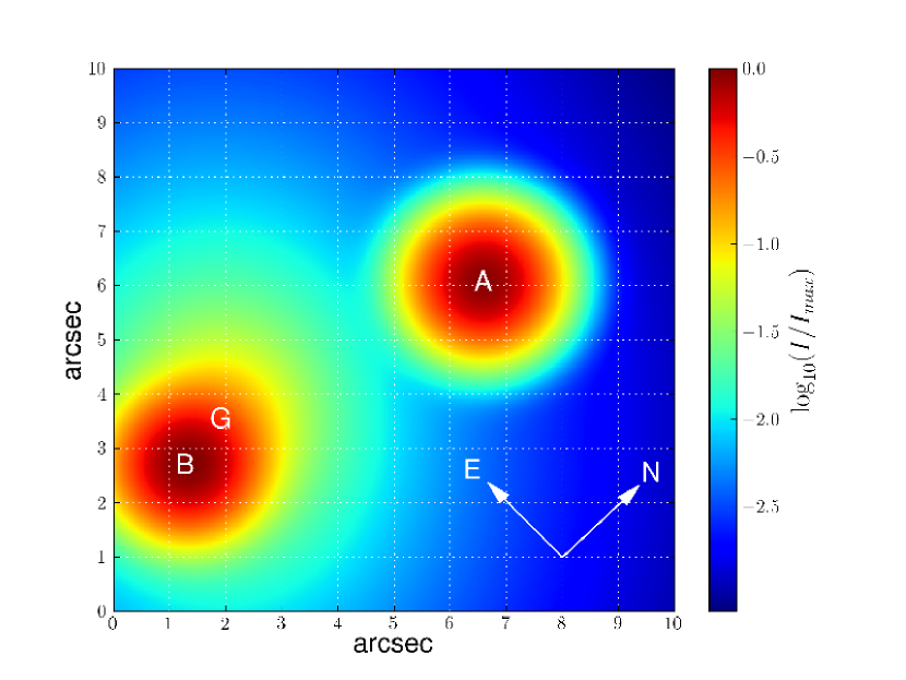
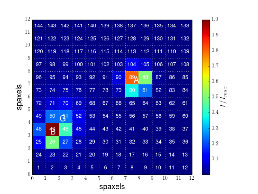
Figure 1: Model of Q0957+561 on the integral field unit of FRODOSpec. Top: the three sources (A, B and G) convolved with a 2D-Gaussian PSF (FWHM = 12). We use astro-photometric data of the system at the reddest optical wavelengths and a simple model for the atmospheric seeing. Bottom: integrated brightness within each lenslet. The whole array contains 144 (12$\times$12) lenslets coupled to fibres. Here, ”spaxels” means spatial pixels.

Due to extended emission in G and atmospheric blurring, there is some level of cross-contamination between the three sources A, B and G. In Fig. 1, we show a model of Q0957+561 on the integral field unit of FRODOSpec (see Sect. 1). This model (simulation) considers all astrometric and photometric properties of the system at the red end of the optical spectrum (A, B and G are of equal brightness), as well as the convolution between source profiles and a two-dimensional Point Spread Function (PSF) having a Gaussian shape with FWHM = 12. Mutual contamination between blurred point-like and extended sources is evident in the top panel of Fig. 1, which displays the brightness distribution on a logarithmic scale. The finite size of the 144 square lenslets also brings a pixelation effect over the field of view. The bottom panel of Fig. 1 shows the integrated brightness within each spatial pixel. After rearranging the fibre bundle in a zigzag pattern (see labels in the bottom panel of Fig. 1), the spectrograph behaves as a linear pseudo-slit.

During the Q0957+561 monitoring program, we have obtained data in many observation sessions using the low-resolution configuration. This configuration enables users to get spectra with wavelength ranges (resolving powers) of 3900$-$5700 Å (2600) and 5800$-$9400 Å (2200) for the blue and red arms. Here, in order to demonstrate the problems of the standard processing pipeline L2 with our science exposures, and the need for a new reduction scheme suitable for blended faint sources in crowded fields, we concentrate on the session on 2011 March 1. Details of the observation log (blue arm) for this night are presented in Table 1. The first letter of the filenames (’b’) refers to the blue arm. Files from the red arm start with the letter ’r’. The second letter of the filenames denotes the target, i.e., ’w’, ’e’ and ’a’ for Tungsten continuum lamp (hereafter W lamp; these exposures are used as flats for tracing fibres), sky target (hereafter q0957 $\equiv$ Q0957+561 or feige34 $\equiv$ Feige 34; feige34 is the calibration star) and Xenon arc lamp (hereafter Xe lamp; exposures for wavelength calibrations), respectively. All blue-arm and red-arm data files may be downloaded from the Gravitational LENses and DArk MAtter (GLENDAMA) website (see Appendix A).

Table 1: Details of the observation log (blue arm) on 2011 March 1

Spectrum	UT	Exposure	Filename (FITS format)
	(hh:mm)	(s)
W lamp	19:22	60	b_w_20110301_2_1_1_1
q0957	21:07	2700	b_e_20110301_7_1_1_2
Xe lamp	21:52	60	b_a_20110301_8_1_1_1
feige34	21:57	100	b_e_20110301_9_1_1_2
Xe lamp	21:59	60	b_a_20110301_10_1_1_1

Notes: q0957 was observed at an air mass of 1.43 and a Moon fraction of 0.08. At the start of observations, the estimated seeing was FWHM = 114. The star (feige34) was observed in similar conditions.

Data taken by FRODOSpec are reduced by two pipelines. The first pipeline, known as L1, is a CCD pre-processing task. L1 performs bias subtraction, overscan trimming and CCD flat fielding. For a sky target in a given arm, the output from L1 is saved as the zero extension in an eight part multi-extension FITS file, e.g., b_e_20110301_7_1_1_2.fits (see Table 1) stores q0957 data in eight extensions [0$-$7], where [0] contains the L1 output. The L1 outputs for q0957 in both spectral arms are shown in Fig. 2. In this figure, the pseudo-slit is oriented along rows (cross-dispersion axis), whereas columns correspond to the dispersion axis. The 144 fibres are located between columns 70 and 1080 in the blue arm, with an inter-fibre space of about 7 pixels (see the top panel of Fig. 2). In the red arm, the fibres are displaced 20 pixels to the right (see the bottom panel of Fig. 2).

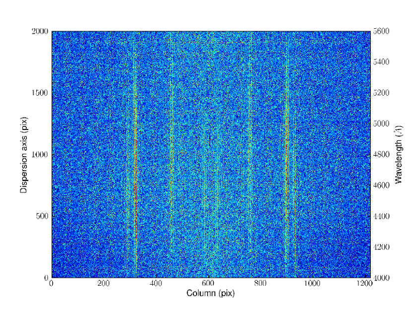
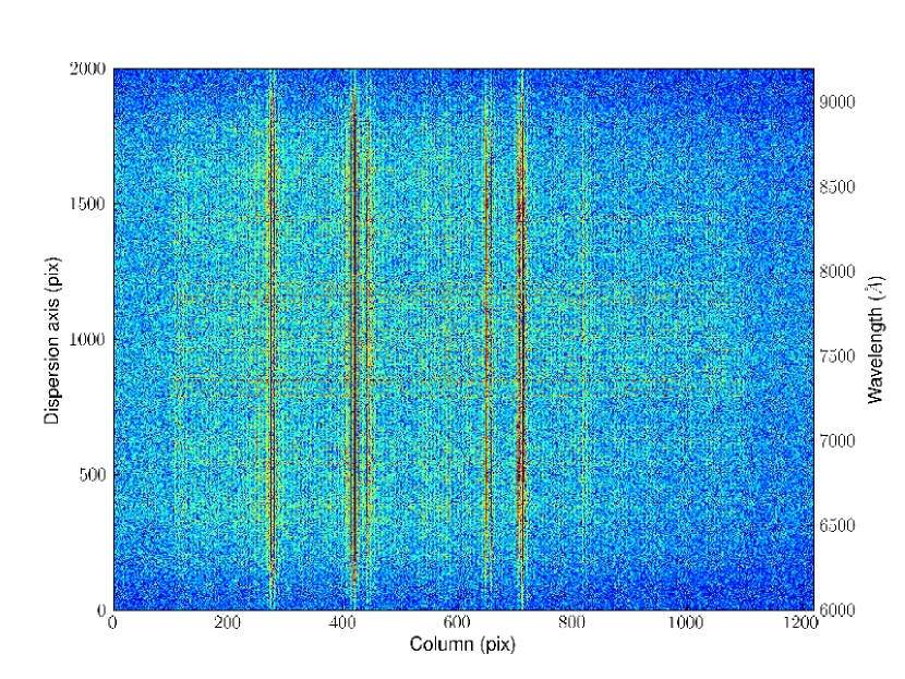
Figure 2: Outputs of the L1 pipeline for q0957. Top: blue spectral arm. Bottom: red spectral arm. See main text for details.

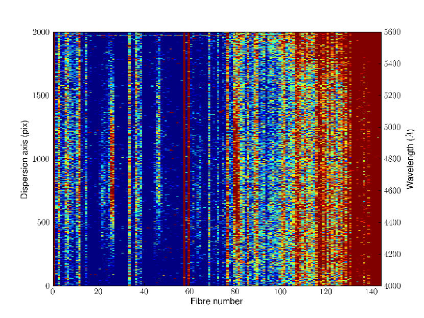
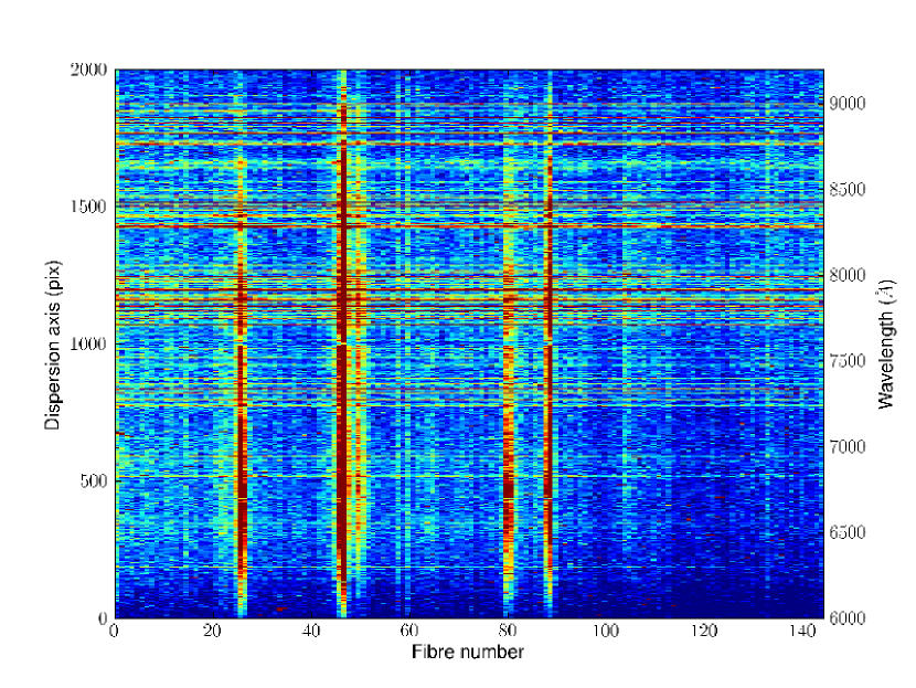
Figure 3: Outputs of the L2 pipeline for q0957. Top: raw spectra (one per fibre) in the blue arm. Bottom: raw spectra in the red arm. See main text for details.

The second pipeline, known as L2, performs the tasks unique to Integral Field Spectroscopy (IFS) reduction, and requires three frames to proceed: a sky target frame (q0957 or feige34), and W and Xe lamp exposures. This standard processing pipeline includes the following main steps (Barnsley et al. 2012):

1. to find and trace the position of each fibre along the dispersion axis (fibre tramline map generation from the W lamp exposure and polynomial fits);

2. to extract the instrumental flux in a 5-pixel aperture around the position of each fibre along the dispersion axis (standard aperture flux extraction in the W and Xe lamp exposures, and the sky target frame using the fibre tramline map);

3. wavelength calibration on a fibre-to-fibre basis (using the Xe lamp spectrum for each fibre);

4. fibre transmission correction (using the W lamp spectrum for each fibre, fibre-to-fibre throughput differences in the sky target spectra are properly corrected);

5. single wavelength solution for all fibres (rebinning the flux along the dispersion axis for each sky target spectrum).

At this stage, the outputs from L2 are saved as the extensions [1] and [2] in the corresponding multi-extension FITS file. For example, b_e_20110301_7_1_1_2.fits[1] contains the 144 wavelength-calibrated spectra for q0957 in the blue arm, while b_e_20110301_7_1_1_2.fits[2] is a spectral data cube. This data cube gives the 2D flux in the 12$\times$12 fibre array at each wavelength pixel. We remark that the [1$-$2] extensions comprise sky-unsubtracted and flux-uncalibrated spectra.

Unfortunately, the results for q0957 are not of sufficient quality, and these can be significantly improved (see Sect. 3). The outputs of the L1 pipeline for q0957 (Fig. 2) clearly show several bright vertical lines associated with the signal from the lens system, whereas the subsequent L2 outputs (one raw spectrum for each fibre on each arm) are rather confusing (Fig. 3). In the bottom panel of Fig. 3, the red light of the science target is gathered near the fibres 26, 47 and 50 (B image plus galaxy), and 80 and 90 (A image), but in the top panel of Fig. 3, is it hard to identify the blue light from the quasar images.

3 Scattered light subtraction and other refinements

It is worth examining more closely the frames in Fig. 2. A detailed look at these L1 outputs reveals two important features. Firstly, there are numerous cosmic rays. As noted by Barnsley et al. (2012), automated removal of cosmic rays from spectrographic data is too unreliable. However, manual removal of cosmic rays with visual inspection of results works quite well. In particular, we have found that the spectral version of the L.A.Cosmic algorithm (van Dokkum 2001) provides good results (see also the PyCosmic algorithm by Husemann et al. 2012). The second feature is more critical. Long exposures (see the exposure time for q0957 in Table 1) lead to high background levels, as shown in Fig. 4. This figure traces the flux curves along the cross-dispersion axis at the central rows of each arm, or more exactly, the spatial distributions of light, averaging over the rows 991$-$1010 in the two spectral arms. Apart from sharp spikes at several columns caused by cosmic rays, there are significant background levels in the fibres between the columns 70 and 1100, the inter-fibre regions (out of the fibre wings), and the fibre-free area encompassing columns 1$-$70 and 1100$-$1220. Hence, we are dealing with scattered (stray) light backgrounds (e.g., Sánchez 2006a), which have not been subtracted by the standard pipeline L2. These 15-count (blue arm) and 7-count (red arm) average background levels (see Fig. 4) can be compared with useful signals in both arms to roughly estimate signal-to-background ratios of about 0.5 (blue arm) and 2 (red arm). In the blue arm, the spectral information is substantially degraded in the presence of large amounts of non-uniformly scattered light. The vertical artefacts apparent in the top panel of Fig. 3 are due to backgrounds in fibres and their (de)magnifications through the step (iv) in L2.

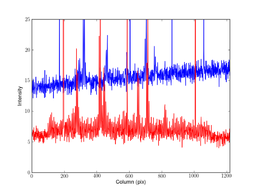
Figure 4: Spatial distributions of light at the central rows of the dispersion axis. Top: blue spectral arm. Bottom: red spectral arm. See main text for details.

We have developed procedures for cleaning the L1 outputs of cosmic rays and scattered light. These procedures are part of a new processing scheme called L2LENS, in which the extraction of fibre spectra is mainly based on the SPECRED package of the Image Reduction and Analysis Facility (IRAF). Apart from IRAF commands, we also use Python scripts to perform reduction tasks. The L2LENS scripts (see Appendix A) are freely available at the GLENDAMA website¹. With respect to the fibre spectrum extraction, the main differences between the standard L2 (Barnsley 2012; Barnsley et al. 2012, and Sect. 2) and the new L2LENS are:

1. cosmic rays are removed by the spectral version of L.A.Cosmic;

2. scattered light subtraction is carried out by means of the IRAF SPECRED/APSCATTER task, which fits a two-dimensional polynomial function to the inter-fibre background. To perform this fit, fifth-order spline functions along the cross-dispersion (columns in Fig. 2) and dispersion (rows in Fig. 2) axes are used;

3. alternative for the step (i) in L2: to trace the fibre positions near the blue end of the red arm, the polynomial order is set to APALL.T_ORDER = 6;

4. alternative for the step (ii) in L2: fibre flux extraction is made by using a 4-pixel aperture rather than the standard one (5 pixels). This procedure tries to avoid the noise in the edges of the standard aperture;

5. wavelength calibration is done in two stages. Firstly, a dispersion solution is found for each fibre independently. A cubic polynomial smoothing is then used to generate a global calibration from the set of 144 initial solutions. In the red arm, the smoothing procedure noticeably reduces fringe effects;

6. fibre-to-fibre and wavelength-to-wavelength throughput differences are corrected. Using the W lamp spectrum for each fibre, an average spectrum is calculated, and then smoothed by a 20-point filter. Individual W lamp spectra are divided by this smoothed (average) spectrum to get correction coefficients for each fibre and wavelength pixel.

At this intermediate stage of L2LENS, its outputs are shown in Fig. 5. These must be compared with the L2 products in Fig. 3. There is a substantial improvement in the blue arm (see the top panels of Fig. 3 and Fig. 5), while changes in the red arm are not so evident. Although a visual inspection of the bottom panels of Fig. 3 and Fig. 5 does not reveal clear differences between both outputs, a quantitative analysis also indicates an appreciable improvement in the red arm with the use of L2LENS. In addition, we can construct spectral data cubes (see Sect. 2). Each data cube consists of 12$\times$12 individual spectra (one per fibre) with 2001 wavelength pixels. The wavelength intervals (dispersions) are 4000$-$5600 Å (0.8 Å/pixel) and 6000$-$9200 Å (1.6 Å/pixel) for the blue and red arms. Here, we do not consider the spectral edges in the wavelength ranges 3900$-$4000, 5600$-$5700, 5800$-$6000 and 9200$-$9400 Å (see the third paragraph in Sect. 2) because they include very noisy, unusable data. Fig. 6 displays the monochromatic frames of q0957 at the central wavelengths of both arms, i.e., 4800 Å (top panel) and 7600 Å (bottom panel).

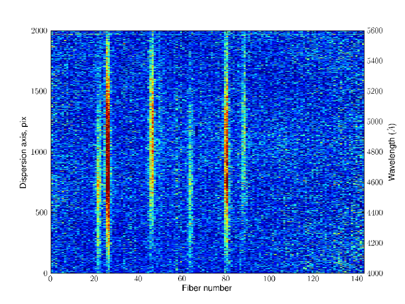
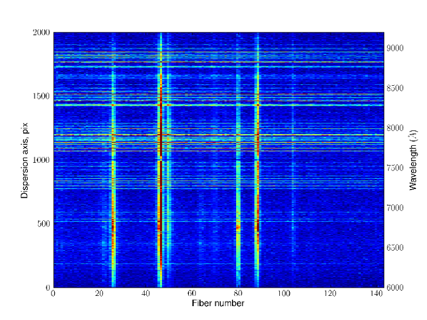
Figure 5: Intermediate outputs of the L2LENS software for q0957. Top: raw spectra (one per fibre) in the blue arm. Bottom: raw spectra in the red arm. See main text for details.

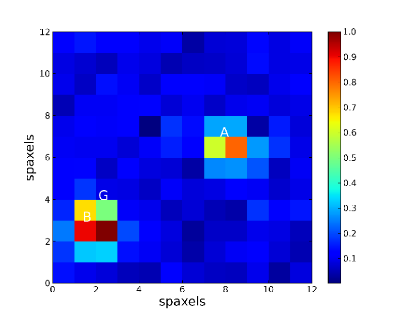
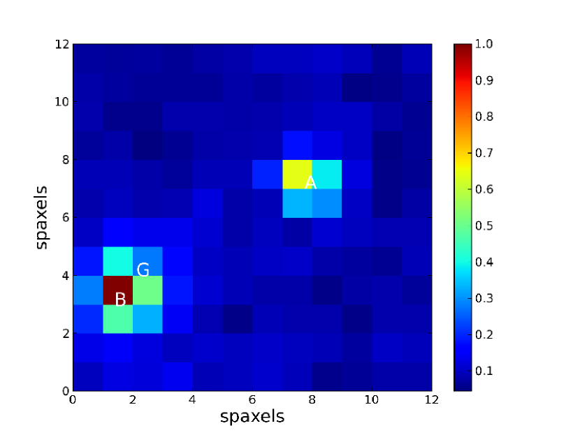
Figure 6: Monochromatic frames of q0957 from the processing scheme L2LENS. Top: $\lambda$ = 4800 Å (blue arm). Bottom: $\lambda$ = 7600 Å (red arm).

4 Flux-calibrated spectra of the lens system

When doing photometry on crowded fields, such as lens systems, aperture photometry does not yield reliable results. It is better to use a PSF fitting method (Wisotzki et al. 2003; Becker et al. 2004; Roth et al. 2004). An additional complication arises as a result of the differential atmospheric refraction, which causes source position variations with wavelength (Filippenko 1982). For example, Arribas et al. (1999) introduced an interpolation procedure to correct these effects in IFS. Our L2LENS software incorporates a PSF fitting task that takes differential atmospheric refraction effects into account.

4.1 PSF fitting method

In order to obtain accurate fluxes for the two quasar images of the lens system q0957, we use a method similar to that presented in Wisotzki et al. (2003). The Wisotzki et al.’s procedure was successfully applied to IFS data of the quadruply lensed quasar HE 0435$-$1223. At each wavelength (monochromatic frame), Wisotzki et al. (2003) decomposed this lens system into four point-like sources (quasar images) convolved with analytical 2D-Gaussian PSFs, plus a spatially constant background. In other words, each quasar image in each monochromatic frame was initially characterised by six free parameters: centroid, FWHM along major and minor axis, position angle and amplitude. However, Wisotzki et al. used some priors to reduce the large number of initial free parameters, and thus, to simplify the $\chi^{2}$ minimization and accurately determine the quasar fluxes. Firstly, the FWHM values were assumed to be the same for all four Gaussians. In a second step, the centroids, FWHM values and position angles were replaced by polynomial functions of $\lambda$, so only the four amplitudes were finally fitted.

Our procedure is a variant of the Wisotzki et al.’s scheme. To model each monochromatic frame, we consider two point-like sources, as well as one extended (de Vaucouleurs profile) source and a uniform background. Hence, our model accounts for the presence of the lensing galaxy. All three sources are convolved with the same PSF, and the first step is to decide on the most suitable shape of this convolution function. For example, Sánchez et al. (2006b) used an empirical PSF that was derived from a standard star. Unfortunately we find significant changes in the PSF with observing time, so the PSF of standard stars can not be incorporated into the model of the lens system. Whereas Wisotzki et al. (2003) used a 2D-Gaussian PSF, sometimes a Moffat profile is a better approach in IFS (Cairós et al. 2012; Kamann et al. 2013). Thus, in order to determine the optimal analytic shape of the PSF, we fit a red frame ($\lambda$ = 7600 Å) of the calibration star feige34 to different profiles. Fig. 7 shows the observed radial profile of feige34 together with the fitted curves: Gaussian (dashed line), Moffat with $\beta$ (power-law index) = 2.5 (dotted line), and Moffat with an arbitrary $\beta$ (solid line). As can be seen in Fig. 7, the Gaussian curve underestimates the flux in the 15$-$3 interval and overestimates the background level, but the Moffat curves work much better. The best fit corresponds to a Moffat profile with $\beta$ = 2.9 (solid line), and we choose a $\beta$ = 3 Moffat distribution to model the PSF in the region of interest (lens system).

Once the PSF shape is chosen, we also use an iterative fitting procedure. The positions of the B image and the lensing galaxy (G) relative to the A image, and the de Vaucouleurs profile of G are set to accurate values from HST observations (Bernstein et al. 1997; Keeton et al. 1998; Kochanek et al. 2013). Therefore, each monochromatic frame of q0957 is initially modelled by a ten-parameter distribution of light. These parameters are the centroid of A, the FWHM along major and minor axis, the position angle of the major axis, the orientation of the frame, the uncalibrated fluxes of A, B and G, and the background sky level. In a subsequent step, the first five parameters of each frame are set to the corresponding values of smoothly varying polynomial functions of $\lambda$, leaving only the three uncalibrated fluxes and the sky level to be fitted (the orientation of the frame is set to the median of all orientations from the initial fits). For calibration purposes, we present the FRODOSpec spectral response function in Sect. 4.2. In Sect. 4.3 we dive into detail on the PSF fitting task, and obtain the flux-calibrated spectra of A, B and G.

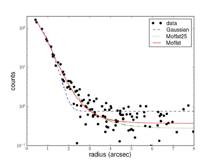
Figure 7: Radial profile of the star feige34: observational data (circles), Gaussian fit (dashed line), $\beta$ = 2.5 Moffat fit (dotted line) and general Moffat fit (solid line).

4.2 FRODOSpec spectral response function

PSF fitting is carried out on both the calibration star and the gravitational lens system. The calibration star model is defined by a single $\beta$ = 3 Moffat distribution (see Sect. 4.1) with a flux peak at ($x_{\rm{S}}$, $y_{\rm{S}}$), widths $\sigma_{x}$ and $\sigma_{y}$, a position angle of the major axis $\theta$, and a total flux $f_{\rm{S}}$. If ($\hat{x}$, $\hat{y}$) is a coordinate system centered on the flux peak, and aligned with the major and minor axes,

$$\hat{x}=(x-x_{\rm{S}})\cos\theta-(y-y_{\rm{S}})\sin\theta$$ (1)

$$\hat{y}=(x-x_{\rm{S}})\sin\theta+(y-y_{\rm{S}})\cos\theta,$$ (2)

and the Moffat distribution with power-law index $\beta$ is given by

$$M(x,y)=f_{\rm{S}}\frac{\beta-1}{\pi\sigma_{x}\sigma_{y}}\left(1+r^{2}(x,y)\right)^{-\beta},$$ (3)

where

$$r(x,y)=\sqrt{\frac{\hat{x}^{2}}{\sigma_{x}^{2}}+\frac{\hat{y}^{2}}{\sigma_{y}^{2}}}.$$ (4)

For $\beta=3$, FWHM_x = 1.02 $\sigma_{x}$ and FWHM_y = 1.02 $\sigma_{y}$. The six parameters of $M(x,y)$ are calculated in an iterative manner. In the first iteration, both spectral data cubes (blue and red arms) with 12$\times$12$\times$2001 pixel³ each are split into 40 slices along the spectral axis. In each slice, 50 adjacent monochromatic frames are combined to increase the signal-to-noise ratio. In order to reduce sampling biases in $M(x,y)$ fitting, each of the 12$\times$12 spatial pixels (or spaxels) is divided into 10$\times$10 equally-sized square subpixels, and the flux distribution in Eq. 3 is evaluated on the 120$\times$120 subpixels of the fine mesh. A flux value for each fibre is then obtained by integrating over the associated spaxel (see Fig. 1). Our $\chi^{2}$ minimization procedure is based on the Levenberg-Marquardt algorithm. This calculates the six Moffat parameters ($x_{\rm{S}}$, $y_{\rm{S}}$, $\sigma_{x}$, $\sigma_{y}$, $\theta$, and $f_{\rm{S}}$) plus a uniform background. In the top panel of Fig. 8, chromatic changes in the flux peak position are due to differential atmospheric refraction, since the measurements of ($x_{\rm{S}}$, $y_{\rm{S}}$) can be accounted for in terms of this atmospheric effect (dashed lines). In the middle panel of Fig. 8, we do not see the expected monotonic decrease of $\sigma_{x}$ with wavelength (blue and cyan squares). We note that the discontinuity does not appear in the $\sigma_{x}$ values from the lens system data (see below). Moreover, the anomaly is only observed some nights. At present, we are trying to find the origin of this time-dependent anomalous behaviour.

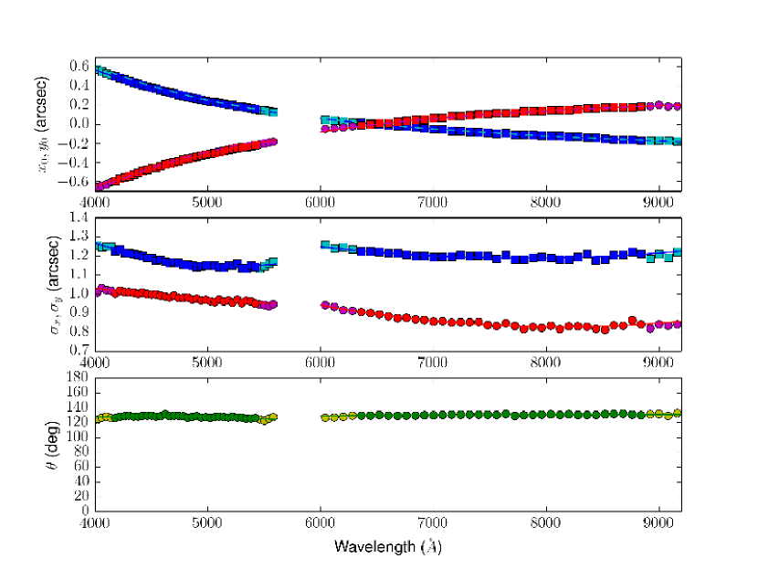
Figure 8: PSF fitting results for 40 (blue arm) + 40 (red arm) spectral slices of feige34 data. The five position-structure parameters of the Moffat distribution are fitted to smooth polynomial functions, excluding the spectral edges in magenta, cyan and yellow (solid lines). In the top panel, we present the flux peak position ($x_{\rm{S}}$, $y_{\rm{S}}$) relative to that at $\lambda$ = 6500 Å. We also show the expected values according to Filippenko (1982) (dashed lines). See main text for details.

In a second iteration, the first five Moffat parameters are fitted to smooth polynomial functions of $\lambda$ (see solid lines in Fig. 8). The position-structure parameters for each monochromatic frame are then evaluated through these polynomial functions, leaving only the uncalibrated flux and background as free parameters. Once we know the uncalibrated spectrum of feige34, $f_{\rm{S}}(\lambda)$, it is possible to build the spectral response function of the spectrograph $S(\lambda)$. This instrumental response is defined as the ratio between the detection rate in counts per second per dispersion pixel, i.e., $f_{\rm{S}}(\lambda)/T_{\rm{S}}$ ($T_{\rm{S}}$ is the exposure time), and the energy flux in erg per square centimetre per second per Å at the entrance of the telescope, $F_{\rm{S}}^{*}(\lambda)$. From the extra-atmospheric energy flux of feige34 (e.g., Oke 1990), $F_{\rm{S}}(\lambda)$, we derive

$$S(\lambda)=\frac{f_{\rm{S}}(\lambda)}{F_{\rm{S}}(\lambda)T_{\rm{S}}10^{-0.4X_{\rm{S}}E(\lambda)}},$$ (5)

where $X_{\rm{S}}$ is the mean airmass during the observation of the calibration star, and $E(\lambda)$ is the standard atmospheric extinction curve at the Roque de los Muchachos Observatory (King 1985). Fig. 9 presents the instrumental response in Eq. 5. The sensitivities at blue wavelengths (blue line) are appreciably lower than those at red wavelengths (red line). A smoothed response function is also plotted in Fig. 9 (green line). We use a 5-point filter in both arms. The red part of $S(\lambda)$ contains several noteworthy features. Apart from fringe effects, there is a striking loss of spectral sensitivity near 6900, 7300, 7600 and 8800 Å. We remark that the standard extinction curve (King 1985) does not account for telluric absorption by molecular oxygen and water vapour. This produces, e.g., the telluric oxygen artefacts near 6900 and 7600 Å. In order to correct the molecular absorption bands, one must divide Eq. 5 by a molecular absorption curve $\epsilon_{\rm{S}}(\lambda)$.

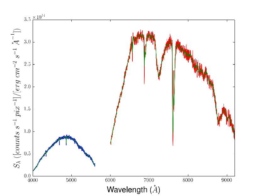
Figure 9: FRODOSpec response function from feige34 data.

4.3 Results

The key ideas to extract the final q0957 spectra are outlined in Sect. 4.1. The lens system model consists of two $\beta$ = 3 Moffat distributions, as well as a de Vaucouleurs profile convolved with a $\beta$ = 3 Moffat PSF. To avoid boundary biases, this last numerical convolution is calculated in a square area nine times larger than the field of view. In a first iteration, we fit the centroid of the A image ($x_{\rm{A}}$, $y_{\rm{A}}$), the PSF parameters ($\sigma_{x}$, $\sigma_{y}$, $\theta$), the orientation of the frame, the total fluxes of the two quasar images and the lensing galaxy ($f_{\rm{A}}$, $f_{\rm{B}}$, $f_{\rm{G}}$), and the sky level, to 2D data for different wavelength slices. The data cubes are split into 40 slices along the spectral axis, as done with the stellar data in Sect. 4.2, and the first five parameters are then treated as polynomial functions of $\lambda$ (see Fig. 10). To trace the polynomial laws, we exclude the values in the spectral edges. These excluded values are drawn in magenta, cyan and yellow in Fig. 10. The orientation of the frame is also set to the median value for all wavelength slices. In the top panel of Fig. 10, $y_{\rm{A}}$ is shown with red and magenta circles. Differential atmospheric refraction (dashed lines) causes vertical displacements $\delta y_{\rm{A}}$ exceeding one spatial pixel (= 083; see Fig. 6).

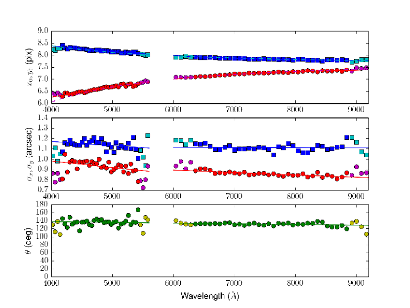
Figure 10: PSF fitting results for 40 (blue arm) + 40 (red arm) spectral slices of q0957 data. The five parameters are also fitted to smooth polynomial functions, excluding the spectral edges in magenta, cyan and yellow (solid lines). Top: $x_{\rm{A}}$ (blue and cyan squares) and $y_{\rm{A}}$ (red and magenta circles). The dashed lines describe the wavelength-dependent displacements of the centroid of the A image arising from differential atmospheric refraction (Filippenko 1982). Middle: $\sigma_{x}$ (blue and cyan squares) and $\sigma_{y}$ (red and magenta circles). Bottom: $\theta$ (green and yellow circles).

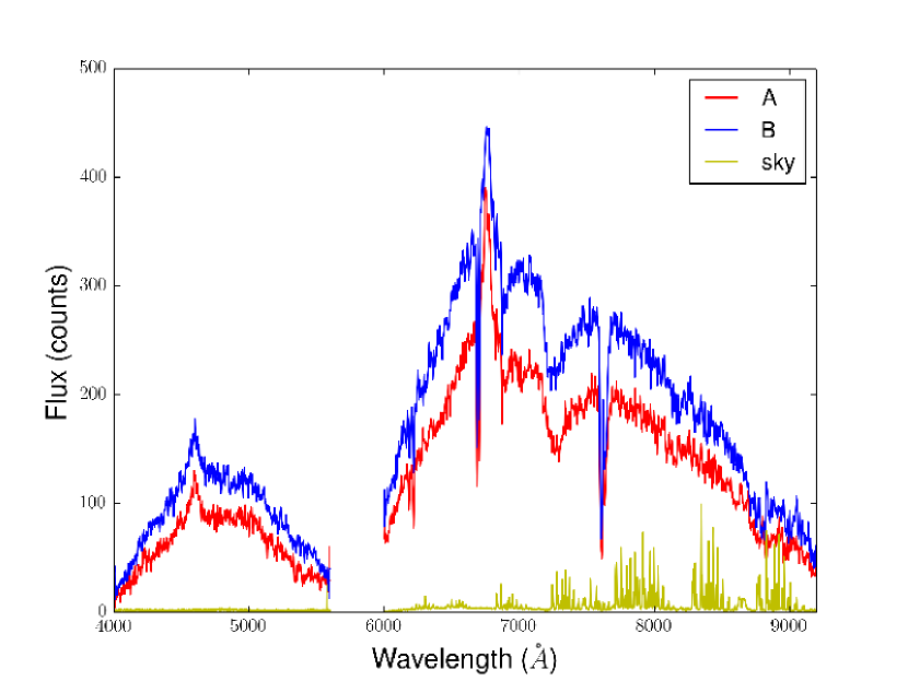
Figure 11: Flux-uncalibrated spectra of the two quasar images A and B. An 8 Å filter is used to smooth the original data. We also display the sky spectrum (counts per spaxel; yellow line) for comparison purposes.

In a second iteration, we only fit $f_{\rm{A}}$, $f_{\rm{B}}$, $f_{\rm{G}}$, and the sky level to each monochromatic frame. The flux-uncalibrated spectra of A and B appear in Fig. 11. Both quasar spectra are smoothed with an 8 Å filter. The galaxy spectrum is very noisy and is not shown in Fig. 11. However, averaging over independent intervals of 400 Å, red-arm fluxes of the galaxy are comparable to quasar fluxes. This result agrees with previous observations of the lens system (e.g., Bernstein et al. 1997; Keeton et al. 1998). The response function $S(\lambda)$ in Eq. 5 and Fig. 9 allows us to calibrate the quasar spectra (Q = A, B):

$$F_{\rm{Q}}(\lambda)=\frac{f_{\rm{Q}}(\lambda)}{S(\lambda)T_{\rm{Q}}10^{-0.4X_{\rm{Q}}E(\lambda)}[\epsilon_{\rm{Q}}(\lambda)/\epsilon_{\rm{S}}(\lambda)]},$$ (6)

where $F_{\rm{Q}}(\lambda)$ is the extra-atmospheric energy flux, $T_{\rm{Q}}$ and $X_{\rm{Q}}$ are the exposure time and airmass for q0957, and $\epsilon_{\rm{Q}}(\lambda)/\epsilon_{\rm{S}}(\lambda)$ is the quasar-to-star molecular absorption ratio. It is assumed that this last ratio is equal to 1, so we must be careful with possible spectral features at typical wavelengths for molecular (telluric) absorption bands. For example, two gray highlighted regions in Fig. 12 correspond to telluric oxygen bands around 6900 and 7600 Å. The calibrated spectra of both quasar images are plotted in Fig. 12 with red (A image) and blue (B image) lines. This figure also includes independent energy fluxes from our photometric monitoring with RATCam in the Sloan $g^{\prime}$ and $r^{\prime}$ bands (Shalyapin et al. 2008). The red (A image) and blue (B image) circles represent the $g^{\prime}r^{\prime}$-Sloan fluxes, which should be compared with spectral fluxes averaged over the $g^{\prime}$ and $r^{\prime}$ broad passbands around 4800 and 6225 Å (see filter responses in Fig. 12). We can not properly asses the calibration in the red arm because our spectra do not cover the full $r^{\prime}$ passband. However, the relative differences in the blue arm do not exceed 7%.

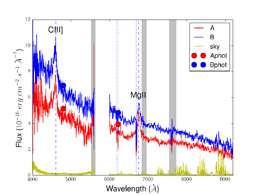
Figure 12: Calibrated spectra of the two quasar images A and B. Both spectra are smoothed with an 8 Å filter (red and blue lines). Energy fluxes from a parallel $g^{\prime}r^{\prime}$-band monitoring are also shown (red and blue circles). Vertical dashed and dotted lines correspond to emission and absorption lines at $z\sim$ 1.4, respectively, whereas the three gray highlighted regions are associated with atmospheric artefacts. Apart from two O₂ (telluric) absorption bands, an imperfect sky extraction likely produces the artefact at 5577 Å. This wavelength corresponds to a strong emission line of atmospheric O i. See main text for details.

The most prominent features of the quasar spectra in Fig. 12 are the C iii] ($\lambda$1909) and Mg ii ($\lambda$2798) emission lines (see the two vertical dashed lines). These are observed around 4600 and 6740 Å ($z_{\rm{Q}}$ = 1.41; Walsh et al. 1979). Going into details, the more accurate and recent value $z_{\rm{Q}}$ = 1.414 (e.g., Rao & Turnshek 2000) is very close to our redshifts from the Mg ii emission line: $z_{\rm{Mg\,{\sc II}}}$(A) = 1.415 and $z_{\rm{Mg\,{\sc II}}}$(B) = 1.416. Additionally, it is well known the existence of a damped Ly$\alpha$ (DLA) system at $z_{\rm{DLA}}$ = 1.391 (e.g., Rao & Turnshek 2000), and redshifts from the Fe ii+Mg ii+Mg i absorption-line complex in our spectra (vertical dotted lines in Fig. 12) deviate only $\delta z$ = 0.001 from $z_{\rm{DLA}}$. These results prove the high precision of the wavelength calibration. In regards to the signal-to-noise ratio (SNR), we obtain SNR $\sim$ 10$-$20 per spectral pixel in the 6300$-$7300 Å continuum. Therefore, averaging over 80 Å intervals (50 pixels), it is achieved $\sim$ 1% accuracy in the red continuum flux. An estimation of the accuracy in the Mg ii emission-line flux is also possible. We obtain a few percent error for this feature.

5 Conclusions

FRODOSpec data of Q0957+561 for a given observation session (2011 March 1) show that the standard processing pipeline L2 (Barnsley et al. 2012) does not yield satisfactory results. We then introduce the new processing scheme L2LENS. This is well suited to the production of spectra of blended faint sources in crowded fields. All L2LENS reduction tasks for the FRODOSpec data on 2011 March 1 are fully detailed in Appendix A. In addition to the user’s guide in Appendix A, our website¹ includes all required data files and Python scripts, as well as several auxiliary files.

Firstly, L2LENS accurately extracts the raw spectrum for each fibre across the field of view. The long exposure of the relatively faint system Q0957+561 is affected by a large number of cosmic rays and significant amounts of scattered light. While the standard pipeline does not account for these artefacts, cleaning of cosmic-ray events and scattered-light backgrounds (and some additional refinements) are incorporated into L2LENS. Secondly, the new processing software allows us to perform PSF fitting photometry on pixels (or broader slices) along the spectral axis, and thus, to infer spectra for the three blended sources of the lens system, i.e., the two quasar images and the lensing galaxy. Our PSF fitting method considers differential atmospheric refraction effects, and it is a variant of the approach by Wisotzki et al. (2003). The final products of L2LENS are the wavelength- and flux-calibrated spectra of both quasar images. Unfortunately, L2LENS does not produce accurate spectrophotometric data for the faint galaxy, whose light is distributed throughout most the field of view. Due to this extended light distribution with an effective radius of 463, the spatial pixels contain a relatively weak signal from the galaxy. To asses the true limits of FRODOSpec, we are currently observing more compact lens systems including fainter quasar images.

The new quasar spectra contain emission and absorption lines whose redshifts deviate $\leq$ 0.002 from the expected ones. Moreover, it is achieved a few percent accuracy in red continuum and Mg ii emission-line fluxes. This demonstrates the big potential of robotic programs with FRODOSpec. We also obtain 1$-$10% uncertainty in image flux ratios in the region of 6300$-$7300 Å, which proves that FRODOSpec is competitive with the Space Telescope Imaging Spectrograph (Goicoechea et al. 2005). We hope that our non-standard FRODOSpec data reduction will stimulate other teams to conduct spectroscopic projects involving relatively faint and/or blended sources (long exposures and/or crowded fields).

Future, relatively large optical telescopes with integral field spectrographs and flexible schedulings will be extraordinarily well suited for surveys/monitorings of blended faint sources with $V\geq$ 20 mag. For example, the successor to the Liverpool Robotic Telescope might be equipped with an improved version of the FRODOSpec spectrograph. This hypothetical integral field unit should have a larger field of view ($\sim$ 1 on sky) and smaller spatial pixels ($\sim$ 01 on sky). The spatial improvements are critical to extract empirical PSFs from field stars and accurately resolve all sources in very crowded fields.

Appendix A L2LENS

This simple User’s Guide describes all steps to successfully process the FRODOSpec observations of Q0957+561 (q0957) and the calibration star Feige 34 (feige34) on 2011 March 1. We assume that /home/user/l2lens is the path to the directory (folder) l2lens. The l2lens folder houses the Python scripts of the L2LENS software, some auxiliary files and the subfolder 110301. All relevant data files of q0957, feige34, and the W and Xe lamps are located in 110301. There is also a sub-subfolder database containing additional auxiliary files. The initial l2lens folder and a README file (explaining its contents; see also here below for a description of the main files and its usage) are freely available at the GLENDAMA website¹. This online material is distributed as a single compressed file l2lens.zip. We also assume that IRAF and Python are properly installed. The Python modules PyRAF, PyFITS, NumPy, SciPy and Matplotlib are needed to run L2LENS scripts.

A.1 Fibre spectrum extraction (IRAF V2.16 + Python 2.7)

For convenience, the pre-processing pipeline (L1) outputs for the blue arm of FRODOSpec are renamed with shorter labels. This is done in 110301, where the data files are found, using the IRAF command lines:

cl> imcopy b_w_20110301_2_1_1_1 bw          Ψ
cl> imcopy b_e_20110301_7_1_1_2.fits[0] be1 Ψ
cl> imcopy b_a_20110301_8_1_1_1 ba1         Ψ
cl> imcopy b_e_20110301_9_1_1_2.fits[0] be2 Ψ
cl> imcopy b_a_20110301_10_1_1_1 ba2

Similar FITS files rw, re1, ra1, re2 and ra2 are produced for the red arm. Here, *w, *e1, *a1, *e2 and *a2 refer to W lamp, q0957, Xe lamp for q0957, feige34 and Xe lamp for feige34, respectively.

The next steps are:

1. Removing cosmic-ray events
   Based on the spectroscopic version of the L.A.Cosmic algorithm⁴. This is put into the extern directory of IRAF (/iraf/iraf/extern), and then

   cl> task lacos_spec = /iraf/iraf/extern/
   lacos_spec.cl
   cl> stsdas
   cl> lacos_spec be1 be1cr be1m.pl
   gain=2.134 readn=3.85 Ψ
   cl> lacos_spec re1 re1cr re1m.pl
   gain=2.350 readn=4.44
   

   A similar procedure is followed for cleaning the feige34 frames be2 and re2. After subtraction of cosmic-ray events, the main FITS files of q0957 and feige34 are be1cr, re1cr, be2cr and re2cr
   

2. Finding and tracing fibre positions along the dispersion axis
   Based on the IRAF/SPECRED package. The command lines are

   cl> noao
   cl> imred
   cl> specred
   cl> apall bw nfind=144 resize- lower=-2
   upper=2 background- minsep=5 maxsep=10
   width=7 weights- clean- t_func="legendre"
   t_step=50 t_niter=1 t_order=3 t_sample=
   "500:2500"
   cl> apall rw nfind=144 t_order=6
   t_sample="1450:3450"
   

   The FITS files bw.ms and rw.ms contain the blue-arm and red-arm W-lamp (continuum emission) spectrum for each fibre
   

3. Removing scattered-light backgrounds
   Based on the IRAF/SPECRED package

   cl> apscatter be1cr be1sc ref=bw
   buffer=0 apscat1.order=5 apscat2.order=5
   apscat2.sample="5:4096" inter-
   

   A similar procedure is followed for cleaning the q0957 frame in the red arm, i.e., re1cr $\to$ re1sc. Now the main FITS files of q0957 are be1sc and re1sc
   

4. Fibre flux extraction
   Based on the IRAF/SPECRED package

   cl> apall be1sc ref=bw out=be1.ms trace-
   recen- intera-
   cl> apall ba1 ref=bw trace- recen-
   intera-
   cl> apall be2cr ref=bw out=be2.ms trace-
   recen- intera-
   cl> apall ba2 ref=bw trace- recen-
   intera-
   

   The FITS file be1.ms (ba1.ms) contains the q0957 (Xe-lamp) spectrum in the blue arm for each fibre, while the file be2.ms (ba2.ms) includes the blue-arm feige34 (Xe-lamp) spectra. Using similar commands, it is also possible to extract spectra in the red arm
   

5. Wavelength calibration (dispersion solution)
   Based on the Python script reident.py

   ./reident.py
   

   This program uses the idba0.ms and idra0.ms files (approximated solutions) in the database sub-subfolder. The lists of Xe emission lines are frodo_blue.dat (blue arm) and frodo_red.dat (red arm). Both lists are available in l2lens. It is necessary to run the Python script four times: name = ’ba1’, ’ba2’, ’ra1’ and ’ra2’ in reident.py
   

6. Throughput correction
   Based on the Python script norm.py

   ./norm.py
   

   Run this script twice: arm = ’b’ and ’r’ in norm.py. The normalized spectrum for each fibre can be found in the FITS files be1nr.ms (q0957/blue arm), re1nr.ms (q0957/red arm), be2nr.ms (feige34/blue arm) and re2nr.ms (feige34/red arm)
   

7. Spectral rebinning (dispersion correction)
   Based on the Python script disp_cor.py

   ./disp_cor.py
   

   Run the script twice: arm = ’b’ and ’r’ in disp_cor.py. This gives the final raw spectrum for each fibre: be1dc.ms (q0957/blue arm), re1dc.ms (q0957/red arm), be2dc.ms (feige34/blue arm) and re2dc.ms (feige34/red arm)
   

8. Making spectral data cubes
   Each data cube gives the 2D flux in the 12$\times$12 fibre array at each wavelength pixel. We use the script rss_cube.py

   ./rss_cube.py
   

   Run the script four times: inname = ’be1’, ’be2’, ’re1’ and ’re2’ in rss_cube.py. This produces the data cubes (FITS files) b1 (q0957/blue arm), r1 (q0957/red arm), b2 (feige34/blue arm) and r2 (feige34/red arm)

A.2 Flux-calibrated spectra of the lens system (Python 2.7)

1. Feige 34: photometry on slices along the spectral axis
   Based on the Python script m2free.py. Both spectral data cubes (b2 and r2) are split into 40 slices along the spectral axis. Each slice is fitted to a seven-parameter model, where the free parameters are: the centroid of the star, the FWHM along major and minor axis, the position angle of the major axis, the uncalibrated flux of the star, and the background sky level. We use the command line ./m2free.py directory x0 y0, where directory refers to the subfolder containing the two data cubes, and x0 y0 is an approximate stellar centroid, i.e.,

   ./m2free.py 110301 6 3
   

   The b2.free and r2.free outputs show 40 solutions each (one per slice)
   

2. Feige 34: polynomial fits to position-structure parameters
   Based on the Python script m2fit.py. The five position-structure parameters are fitted to smooth polynomial functions of wavelength

   ./m2fit.py 110301
   

   The b2.fit and r2.fit outputs show 2001 solutions each (one per dispersion pixel). These fits are displayed in Fig. 8
   

3. Feige 34: photometry on monochromatic frames
   Based on the Python script m2fix.py. Each monochromatic frame is fitted to a two-parameter model. The five position-structure parameters are evaluated through smooth polynomial functions (b2.fit and r2.fit), leaving only the uncalibrated flux and the sky level as free parameters

   ./m2fix.py 110301
   

   The b2.fix and r2.fix outputs show 2001 (stellar flux, sky level) pairs each. These files also include the standard spectral response of FRODOSpec (Fig. 9), which is based on the true spectrum of Feige 34 (f34a.oke in l2lens) and the standard atmospheric extinction curve at the Roque de los Muchachos Observatory (lam_extin.dat in l2lens). The optional script m2graph.py (use the command line ./m2graph.py 110301) also allows the user to check b2.fix and r2.fix
   

4. Lens system: photometry on slices along the spectral axis
   Based on the Python script m1free.py. Both spectral data cubes (b1 and r1) are split into 40 slices along the spectral axis. Each slice is fitted to a ten-parameter model, where the free parameters are: the centroid of Q0957+561A, the FWHM along major and minor axis, the position angle of the major axis, the orientation of the frame, the uncalibrated total fluxes of the two quasar images (Q0957+561A and Q0957+561B) and the lensing galaxy, and the sky level. We use the command line ./m1free.py directory x0 y0, where directory refers to the subfolder containing the two data cubes, and x0 y0 is an approximate centroid of Q0957+561A, i.e.,

   ./m1free.py 110301 8 6.5
   

   The b1.free and r1.free outputs show 40 solutions each (one per slice)
   

5. Lens system: polynomial fits to position-structure parameters and estimation of orientations
   Based on the Python script m1fit.py. The five position-structure parameters are fitted to smooth polynomial functions of wavelength, excluding the spectral edges. For each spectral arm, it is also obtained the median orientation for all wavelength slices

   ./m1fit.py 110301
   

   The b1.fit and r1.fit outputs show 2001 solutions each (one per dispersion pixel). These fits are displayed in Fig. 10. Apart from position-structure data, the outputs contain the orientations of each arm
   

6. Lens system: photometry on monochromatic frames
   Based on the Python script m1fix.py. Each monochromatic frame is fitted to a four-parameter model. The five position-structure data and the frame orientation are taken from the b1.fit and r1.fit files. Thus, only the uncalibrated fluxes and the sky level are free parameters

   ./m1fix.py 110301
   

   The b1.fix and r1.fix outputs include 2001 (flux_A, flux_B, flux_G, sky level) vectors each
   

7. Final spectra of the two quasar images
   Based on the Python script m1graph.py

   ./m1graph.py
   

   The b.dat and r.dat files contain the flux-calibrated spectra of the two quasar images and the lens galaxy (units are described in the main text). The m1graph.py script also produces Fig. 11 and a variant of Fig. 12