Exact recursive estimation of linear systems subject to bounded disturbances

Abstract

This paper addresses the classical problem of determining the sets of possible states of a linear discrete-time system subject to bounded disturbances from measurements corrupted by bounded noise. These so-called uncertainty sets evolve with time as new measurements become available. We present an exact, computationally simple procedure that propagates a point on the boundary of the uncertainty set at some time instant to a set of points on the boundary of the uncertainty set at the next time instant.

siconxxxxxxxx–x

1 Introduction

If a linear, time-invariant dynamic system is driven by set-bounded process noise, and has measurements corrupted with set-bounded observation noise, then the set of current possible states of the system consistent with the measurements up to the current time is termed the state uncertainty set (or simply uncertainty set), or sometimes the guaranteed state estimate. An algorithm for determining the uncertainty set is sometimes called a set-valued observer. This set membership estimation problem is fundamental and has many applications, for example in control under constraints in the presence of noise [2, 10]. It falls under the general topic of set membership uncertainty, see [5]. Recently there has been interest in combining stochastic and set-bounded disturbances [13]. The uncertainty set is needed in all of these applications. Uncertainty set estimation is also closely related to non-stochastic approaches to system identification [8, 21, 25, 27].

The first results on recursive determination of the uncertainty set are in [28, 34, 35]. See also [6]. Since the appearance of these papers there has appeared an extensive literature on the topic; see the survey papers [3, 22].

Most research to date has been on schemes that construct approximations to the uncertainty set, for example [1, 4, 7, 27, 29, 32, 33, 36]. In the system identification literature there are results on exact recursive polytope determination, for example [23], where useful descriptions of evolving polytopic uncertainty sets are given. We have the same goal, but a completely different algorithm. Exact schemes generally have not been suitable for real-time implementation because of their computational complexity. In this paper we present for the first time a procedure that is exact, recursive and computationally simple. When a new measurement arrives, points on the boundary of the uncertainty set at the current time are mapped exactly to points on the boundary of the uncertainty set at the next time instant. The number of points that can be propagated forwards in time this way is restricted only by speed and storage constraints, the computational requirements for propagating one point being very small.

If the process and observation noise are restricted pointwise-in-time by inequality constraints, then with the processing of more measurements the number of vertices possessed by the polytopic uncertainty set may increase, decrease, or stay the same. Each vertex of the uncertainty set at one time instant may be mapped to either zero, one, or two vertices, or to an edge, of the uncertainty set at the next time instant. Even if memory limitations preclude the determination of all vertices, knowing the exact location of a large number of points on the boundary of the uncertainty set potentially will provide useful information in a wide range of applications. Exact determination of the uncertainty set should also be of value in theoretical work and in simulations.

There is a connection between uncertainty set estimation and research on $l_{1}$ optimal control; [24, 31] provide interesting insights on this. In the robustness literature problems with the same number of disturbances as measurements, and the same number of controls as regulated outputs, are referred to as one-block problems. See [17] for a recent discussion of the one-block $l_{1}$ optimal control problem. Our estimation problem has two disturbances, one measurement and, because in this paper we are not attempting the next step of using the estimate for closed-loop feedback, no controls or regulated outputs. It is therefore a 2-block problem, where the disturbances are connected by convolution constraints. As explained in [30], multi-block $l_{1}$ control problems necessarily have convolution constraints, one-block problems have no convolution constraints, and so-called zero-interpolation constraints, which ensure stability of the closed loop system, may or may not be present in multi-block problems. If the measurements in our estimation system are identically zero, the artificial regulator system that we set up and recursively solve is a 2-block $l_{1}$ optimal control row problem with no zero-interpolation conditions. When the measurements are non-zero the cost function for the regulator system is no longer the $l_{1}-$ norm, but it remains piece-wise linear and convex. Thus the heart of our procedure can be interpreted as recursively solving a slight generalization of a 2-block $l_{1}$ optimal control problem. The results in this paper build on some of the ideas in [14, 15, 16].

Although there is no notion of optimality in the definition of uncertainty sets, our procedure is derived using optimization methods. The uncertainty sets are interpreted as feasible sets for specially constructed optimization problems, and optimal solutions to these programs are points on the boundaries of the uncertainty sets.

2 Problem formulation

A linear, time-invariant, causal discrete-time scalar system $\mathbf{z}=P\mathbf{v}+\mathbf{w}$ is depicted in Fig. 1

Fig. 1: Estimation system

where $(v_{k})_{k=1}^{\infty},(z_{k})_{k=1}^{\infty}$ and $(w_{k})_{k=1}^{\infty}$ are, respectively, the input disturbance to the plant $P$, the measurement, and the measurement disturbance sequences. The plant output sequence is $y_{k}=z_{k}-w_{k}.$ It is known a priori that the disturbances satisfy $\left|v_{k}\right|\leq 1$ and $\left|w_{k}\right|\leq 1,$ and the initial state, at time $k=0,$ is given. The restriction of $v_{k}$ and $w_{k}$ to the interval $\left[-1,1\right]$ is made for notational convenience. The method to be described generalizes easily to situations where $v_{k}$ is restricted to intervals of the form $\left[v_{k}^{l},v_{k}^{u}\right],$ and $w_{k}$ to $\left[w_{k}^{l},w_{k}^{u}\right]$, where $v^{l},v^{u},w^{l}$ and $w^{u}$ are a-priori given bounding sequences.

The state-space description best suited to our needs, given below, is related to controllability form. The plant dynamics are also expressible, via the transfer function representation of the system, as convolution constraints relating $v$ and $y$; we shall make use of both of these system representations.

The problem addressed is: Given the a priori information on $w_{1},\ldots,w_{k},v_{1},\ldots,v_{k},$ the initial state $\mathbf{x}_{0},$ the measurement history $z_{1},\ldots,z_{k},$ and the plant dynamics, what are the possible states at time $k,$ immediately after the measurement $z_{k}$ has been received? The set of all such states, termed the uncertainty set at time $k,$ will be denoted $S_{k},$ a convex polytope in $\mathbb{R}^{m},$ where $m$ is the order (McMillan degree) of the plant. Determining the set $S_{k}$ is an estimation problem, and we shall refer to the system in Fig. 1 as the estimation system.

2.1 Notation and preliminaries

The boundary and interior of a set $S$ are denoted $\partial S$ and $\operatorname*{int}S$, and $\emptyset$ denotes the empty set. The support function of a convex, bounded non-empty subset $S$ of $\mathbb{R}^{m}$ is $h_{S}(\mathbf{x}^{\ast})=\sup_{\mathbf{x}\in S}\left\langle\mathbf{x}^{\ast},\mathbf{x}\right\rangle,$ where $\mathbf{x}^{\ast}\in\mathbb{R}^{m}.$ The cone $\left\{\mathbf{x}^{\ast}:\left\langle\mathbf{x}^{\ast},\mathbf{x}\right\rangle=h_{S}(\mathbf{x}^{\ast}),\text{ }\mathbf{x}^{\ast}\neq\mathbf{0}\right\}$ associated with $\mathbf{x}\in\partial S$ is denoted $C_{S}^{O}\left(\mathbf{x}\right).$ Given a vector $\mathbf{y=}\left(y_{1},y_{2},\ldots\right)$ and any $s\in\mathbb{N}^{+},$ $t\in\mathbb{N}^{+}$ satisfying $s<t,$ we denote $\left(y_{s},y_{s+1},\ldots,y_{t}\right)$ by $y_{s:t}.$ In matrix equations vectors are by default column vectors, so for example $y_{s:t}$ occuring in a matrix equation would be a column vector, and $y_{s:t}^{T}$ is a row vector, where the superscript $T$ denotes transpose. The vector of length $t+1$ whose first $t$ components are $y_{1:t}$ and whose last component is the scalar $y$ is denoted $\left(y_{1:t},y\right).$ The $\lambda$-transform (generating function) of an arbitrary sequence $\mathbf{y}=(y_{k})_{k=1}^{\infty}$ is defined to be $\hat{y}(\lambda):=\sum_{k=1}^{\infty}y_{k}\lambda^{k-1}.$ Let $\mathbf{d}=d_{1:m+1}=(d_{1},\ldots,d_{m+1})$ and $\mathbf{n}=n_{1:m+1}=(n_{1},\ldots,n_{m+1}),$ $m\geq 1,$ be real vectors. The Toeplitz Bezoutian $B_{T}(\mathbf{n},\mathbf{d})=\left(b_{ij}\right)_{i,j=1}^{m}$ of the vectors $\mathbf{n},\mathbf{d}$ (or the polynomials $\hat{\mathbf{n}},\hat{\mathbf{d}}$) is the $m\times m$ matrix with the generating polynomial

(1) $$\sum_{i,j=1}^{m}b_{ij}t^{i-1}s^{j-1}=\frac{s^{m}\hat{\mathbf{n}}\left(1/s\right)\hat{\mathbf{d}}\left(t\right)-s^{m}\hat{\mathbf{d}}\left(1/s\right)\hat{\mathbf{n}}\left(t\right)}{1-st}.$$

Denote by $D$ and $N$ the infinite, banded, lower-triangular Toeplitz matrices whose first columns are $\mathbf{d}$ and $\mathbf{n}$, respectively. Define the following submatrices of $D$ and $N$

$$D_{L}:=\left[\begin{array}[c]{cccc}d_{1}&0&\cdots&0\\ d_{2}&d_{1}&\ddots&\vdots\\ \vdots&\ddots&\ddots&0\\ d_{m}&\cdots&d_{2}&d_{1}\end{array}\right]\qquad D_{U}:=\left[\begin{array}[c]{cccc}d_{m+1}&d_{m}&\cdots&d_{2}\\ 0&d_{m+1}&\ddots&\vdots\\ \vdots&\ddots&\ddots&d_{m}\\ 0&\cdots&0&d_{m+1}\end{array}\right]$$

$$N_{L}:=\left[\begin{array}[c]{cccc}n_{1}&0&\cdots&0\\ n_{2}&n_{1}&\ddots&\vdots\\ \vdots&\ddots&\ddots&0\\ n_{m}&\cdots&n_{2}&n_{1}\end{array}\right]\qquad N_{U}:=\left[\begin{array}[c]{cccc}n_{m+1}&n_{m}&\cdots&n_{2}\\ 0&n_{m+1}&\ddots&\vdots\\ \vdots&\ddots&\ddots&n_{m}\\ 0&\cdots&0&n_{m+1}\end{array}\right].$$

More generally, for any $k>0,$ the $k\times k$ upper left hand corner submatrix of $D$ is denoted $D_{k}.$ The matrix $N_{k}$ is defined similarly. Thus $D_{m}=D_{L}$ and $N_{m}=N_{L}.$

One form of the Gohberg-Semencul formulas [9, 11] states

(2) $$B_{T}(\mathbf{n},\mathbf{d})=D_{L}N_{U}-N_{L}D_{U}=N_{U}D_{L}-D_{U}N_{L},$$

and $B_{T}(\mathbf{n},\mathbf{d})$ is invertible if and only if $\hat{\mathbf{n}}$ and $\hat{\mathbf{d}}$ are coprime. From now on we abbreviate $B_{T}(\mathbf{n},\mathbf{d})$ to $B_{T},$ and $B_{T}^{-1}$ is the inverse of $B_{T}.$ The first row of $B_{T}$ plays an important role and will be denoted by $C,$ so $C:=\left(d_{1}\left[\begin{array}[c]{c}n_{m+1}\\ \vdots\\ n_{2}\end{array}\right]-n_{1}\left[\begin{array}[c]{c}d_{m+1}\\ \vdots\\ d_{2}\end{array}\right]\right)^{T}$. See [12] for properties of Bezoutians.

2.2 Transfer function description

The plant for the estimation system has the transfer function representation $P(\lambda)=\hat{\mathbf{n}}(\lambda)/\hat{\mathbf{d}}(\lambda)$ where

(3) $$\hat{\mathbf{n}}(\lambda) =n_{1}+n_{2}\lambda+n_{3}\lambda^{2}+\cdots+n_{m+1}\lambda^{m}$$

$$\hat{\mathbf{d}}(\lambda) =1+d_{2}\lambda+d_{3}\lambda^{2}+\cdots+d_{m+1}\lambda^{m},$$

$m\geq 1$ is an integer, $\hat{\mathbf{n}}(\lambda)$ and $\hat{\mathbf{d}}(\lambda)$ are assumed to be coprime polynomials with real coefficients, and it is assumed that both the plant $P(\lambda)$ and the plant $P^{\ast}(\lambda)$ for the regulator system, defined below, are causal, implying $d_{1}\neq 0$ and $d_{m+1}\neq 0$. Without loss of generality we take $d_{1}=1.$ Assuming zero initial conditions, $\mathbf{y}$ and $\mathbf{v}$ are related by

(4) $$\hat{\mathbf{d}}(\lambda)\hat{y}(\lambda)=\hat{\mathbf{n}}(\lambda)\hat{v}(\lambda),$$

or equivalently $\mathbf{d}\ast\mathbf{y}=\mathbf{n}\ast\mathbf{v},$ where $\ast$ denotes convolution.

Equating like powers of $\lambda$ on both sides of (4), and allowing the possibility of non-zero initial conditions, we have

(5) $$D\mathbf{y}-N\mathbf{v}=\left[\begin{array}[c]{c}D_{L}y_{1:m}-N_{L}v_{1:m}\\ 0\end{array}\right].$$

Equations (5) describe how the signals $\mathbf{y}$ and $\mathbf{v}$ are related in the estimation system. In the state-space representation to be introduced next, $B_{T}^{-1}\left(D_{L}y_{1:m}-N_{L}v_{1:m}\right)$ is the initial state $\mathbf{x}_{0}.$

2.3 State-space representations

The state-space description of the estimation system we employ is sometimes denoted second controllability canonical form ([19], p 293). It is

$$\mathbf{x}_{k} =A\mathbf{x}_{k-1}+Bv_{k}$$

(6) $$y_{k} =C\mathbf{x}_{k-1}+D_{1}v_{k}$$

$$z_{k} =y_{k}+w_{k}$$

where

(7f) $$A =\left[\begin{array}[c]{cc}0&I_{m-1}\\ -d_{m+1}&\begin{array}[c]{cc}\cdots&-d_{2}\end{array}\end{array}\right],\text{ }B=\left[\begin{array}[c]{c}0\\ 1\end{array}\right],$$

(7m) $$C^{T} =\left[\begin{array}[c]{c}n_{m+1}\\ \vdots\\ n_{2}\end{array}\right]-\left[\begin{array}[c]{c}d_{m+1}\\ \vdots\\ d_{2}\end{array}\right]n_{1},\text{ }D_{1}=n_{1};$$

and

(8) $$\mathbf{x}_{k}=\mathbf{x}_{k}(\mathbf{y},\mathbf{v}):=\left\{\begin{array}[c]{c}B_{T}^{-1}\left[D_{L}y_{k+1:k+m}-N_{L}v_{k+1:k+m}\right]\text{ for }k\geq 0\\ B_{T}^{-1}\left[-D_{U}y_{k-m+1:k}+N_{U}v_{k-m+1:k}\right]\text{ for }k\geq m\end{array}\right..$$

In (7) $I_{m-1}$ denotes the $m-1$ dimensional identity matrix, and $0$ denotes a column vector of zeros of length $m-1$. The fact that $D_{L}y_{k+1:k+m}-N_{L}v_{k+1:k+m}=-D_{U}y_{k-m+1:k}+N_{U}v_{k-m+1:k}$ for $k\geq m$ follows from (5).

We will also require a state-space realization of a related system, which we shall refer to as the regulator system. The input and output sequences are respectively $(y_{k}^{\ast})_{k=1}^{\infty}$ and $(v_{k}^{\ast})_{k=1}^{\infty},$ and the plant regulator system, denoted $P^{\ast},$ has the transfer function representation

(9) $$P^{\ast}(\lambda)=-\frac{\mathbf{\tilde{n}}(\lambda)}{\mathbf{\tilde{d}}(\lambda)}$$

where $\mathbf{\tilde{n}}=\left(n_{m+1},\ldots,n_{1}\right)$ and $\mathbf{\tilde{d}}=\left(d_{m+1},\ldots,d_{1}\right).$ A minimal state-space realization of the regulator system is

(10) $$\mathbf{x}_{k}^{\ast} =A^{\ast}\mathbf{x}_{k-1}^{\ast}+B^{\ast}y_{k}^{\ast}$$

(11) $$v_{k}^{\ast} =C^{\ast}\mathbf{x}_{k-1}^{\ast}+D_{1}^{\ast}y_{k}^{\ast}$$

(24) $$A^{\ast} =\left[\begin{array}[c]{cc}-d_{m}/d_{m+1}&I_{m-1}\\ \begin{array}[c]{c}\vdots\\ -1/d_{m+1}\end{array}&\begin{array}[c]{c}\\ 0\end{array}\end{array}\right],\text{ }B^{\ast}=\left[\begin{array}[c]{c}n_{m}\\ \vdots\\ n_{1}\end{array}\right]-\left[\begin{array}[c]{c}d_{m}\\ \vdots\\ 1\end{array}\right]\frac{n_{m+1}}{d_{m+1}},$$

(26) $$C^{\ast} =\left[\begin{array}[c]{cccc}-1/d_{m+1}&0&\cdots&0\end{array}\right],\text{ }D_{1}^{\ast}=\frac{-n_{m+1}}{d_{m+1}};$$

and

(27) $$\mathbf{x}_{k}^{\ast}=\mathbf{x}_{k}^{\ast}(\mathbf{y}^{\ast},\mathbf{v}^{\ast}):=\left\{\begin{array}[c]{c}-N_{U}^{T}y_{k+1:k+m}^{\ast}-D_{U}^{T}v_{k+1:k+m}^{\ast}\text{ for }k\geq 0\\ N_{L}^{T}y_{k-m+1:k}^{\ast}+D_{L}^{T}v_{k-m+1:k}^{\ast}\text{ for }k\geq m\end{array}\right.,$$

where $\mathbf{x}_{k}^{\ast}$ is the regulator state at time $k$. From (9) we have $\mathbf{\tilde{n}}\ast\mathbf{y}^{\ast}+\mathbf{\tilde{d}}\ast\mathbf{v}^{\ast}=\left(\left[y_{1:m}^{\ast}\right]^{T}N_{U}+\left[v_{1:m}^{\ast}\right]^{T}D_{U},0,\ldots\right)^{T}$ where the first component of the right hand side vector is $-\mathbf{x}_{0}^{\ast}.$ These state-space representations are in principle well known [18, 19, 26].

2.4 The uncertainty set and worst-case disturbances

The estimation system at time zero is in the state $\mathbf{x}_{0},$ so $D_{L}y_{1:m}-N_{L}v_{1:m}=B_{T}\mathbf{x}_{0}.$ From the input-output description (5), after $k\geq 2m$ measurements have been processed $y_{1:k}$ and $v_{1:k}$ are related by

(28) $$\left[\begin{array}[c]{cccc}D_{L}&&&\\ D_{U}&D_{L}&&\\ &\ddots&\ddots&\\ &&D_{U}&D_{L}\end{array}\right]\left[\begin{array}[c]{c}y_{1}\\ \vdots\\ y_{k}\end{array}\right]-\left[\begin{array}[c]{cccc}N_{L}&&&\\ N_{U}&N_{L}&&\\ &\ddots&\ddots&\\ &&N_{U}&N_{L}\end{array}\right]\left[\begin{array}[c]{c}v_{1}\\ \vdots\\ v_{k}\end{array}\right]=\left[\begin{array}[c]{c}B_{T}\mathbf{x}_{0}\\ 0\\ \vdots\\ 0\end{array}\right],$$

where here and later it is not necessarily the case that $k$ be an integer multiple of $m.$ In the notation of Section 2.1, (28) is $D_{k}y_{1:k}-N_{k}v_{1:k}=\left[\begin{array}[c]{cccc}B_{T}\mathbf{x}_{0}&0&\cdots&0\end{array}\right]^{T}.$ The uncertainty set $S_{k}$ is then given by

(29) $$S_{k}=\left\{\begin{array}[c]{c}\mathbf{x}\in\mathbb{R}^{m}:B_{T}\mathbf{x=}B_{T}\mathbf{x}_{k}(\mathbf{y},\mathbf{v})=-D_{U}y_{k-m+1:k}+N_{U}v_{k-m+1:k},\\ \left\|v_{1:k}\right\|_{\infty}\leq 1,\left\|y_{1:k}-z_{1:k}\right\|_{\infty}\leq 1,\text{ and (\ref{conv_lengthk}) holds.}\end{array}\right\}$$

Following Witsenhausen, [35], $S_{k}$ is given recursively in terms of $S_{k-1}$ and the new observation $z_{k}$ by

(30) $$S_{k}=\left\{\begin{array}[c]{c}\mathbf{x}_{k}:\mathbf{x}_{k-1}\in S_{k-1},\text{ }\mathbf{x}_{k}=A\mathbf{x}_{k-1}+Bv_{k},\text{ }y_{k}=C\mathbf{x}_{k-1}+D_{1}v_{k},\\ \left|v_{k}\right|\leq 1,\text{ }\left|y_{k}-z_{k}\right|\leq 1.\end{array}\right\}$$

For states $\mathbf{x}_{k-1}$ and $\mathbf{x}_{k}$ related as in (30) we shall say that $\mathbf{x}_{k-1}$ is a precursor of $\mathbf{x}_{k}$, and $\mathbf{x}_{k}$ is a successor to $\mathbf{x}_{k-1}.$

Definition 1.

The state $\mathbf{x}_{k-1}\in S_{k-1}$ is said to be a precursor of the state $\mathbf{x}_{k}\in S_{k},$ $\mathbf{x}_{k-1}$ is propagated to $\mathbf{x}_{k},$ and $\mathbf{x}_{k}$ is a successor to $\mathbf{x}_{k-1},$ if there exists a scalar $v$ satisfying $\left|v\right|\leq 1$ and $\left|C\mathbf{x}_{k-1}+D_{1}v-z_{k}\right|\leq 1$ for which $\mathbf{x}_{k}=A\mathbf{x}_{k-1}+Bv$.

Clearly every $\mathbf{x}_{k}\in S_{k}$ is a successor to some $\mathbf{x}_{k-1}\in S_{k-1}.$ The following Proposition follows directly from the preceding definitions.

Proposition 2.

The vector $\mathbf{x}_{k}$ is a successor to $\mathbf{x}_{k-1}$ if and only if there exists $(y_{1:k},v_{1:k})$ satisfying (28), $\left\|v_{1:k}\right\|_{\infty}\leq 1,$ $\left\|y_{1:k}-z_{1:k}\right\|_{\infty}\leq 1,$ $\mathbf{x}_{k}=\mathbf{x}_{k}\left(y_{1:k},v_{1:k}\right)$ and $\mathbf{x}_{k-1}=\mathbf{x}_{k-1}\left(y_{1:k},v_{1:k}\right).$

At time $k$ any state $\mathbf{x}_{k}\in S_{k}$ is associated with possibly non-unique disturbance histories $v_{1:k}$ and $w_{1:k}.$ Specifying one of the disturbance histories uniquely determines the other, if the measurement history $z_{1:k}$ and the initial state $\mathbf{x}_{0}$ are known. Thus the state at time $k$ can be expressed in terms of the initial state and $v_{1:k}.$ From (6) we have

(31) $$\mathbf{x}_{k} =A^{k}\mathbf{x}_{0}+{\displaystyle\sum\limits_{j=0}^{k-1}}A^{j}Bv_{k-j}$$

(32) $$w_{k} =z_{k}-CA^{k-1}\mathbf{x}_{0}-C{\displaystyle\sum\limits_{j=0}^{k-2}}A^{j}Bv_{k-j-1}-D_{1}v_{k}.$$

Every state $\mathbf{x}_{k}$ on the boundary of $S_{k}$ is determined, through (31), by a so-called “worst-case” disturbance sequence $v_{1:k}$.

Definition 3.

The signal $v_{1:k}$ is said to be a worst-case disturbance associated with $\mathbf{x}_{k}$ if $\mathbf{x}_{k}$ given by (31) satisfies $\mathbf{x}_{k}\in\partial S_{k}.$

We will also say $\left(w_{1:k},v_{1:k}\right)$ are worst-case disturbances associated with $\mathbf{x}_{k}$ if $v_{1:k}$ is a worst-case disturbance associated with $\mathbf{x}_{k}$ and (32) holds.

In [35] primal and dual recursive procedures based on (30) are derived; they require manipulations of sets, a computationally difficult task. Our recursion operates not on the whole set $S_{k-1}$, but rather only on those boundary points of $S_{k-1}$ that are precursors of boundary points of $S_{k}.$ We also apply the equation $\mathbf{x}_{k}=A\mathbf{x}_{k-1}+Bv_{k},$ but only after first identifying all suitable $v_{k}.$ By this is meant, for a given $\mathbf{x}_{k-1}\in S_{k-1},$ finding all $v_{k}$ satisfying $\left|v_{k}\right|\leq 1,$ $\left|y_{k}-z_{k}\right|\leq 1$ having the property $A\mathbf{x}_{k-1}+Bv_{k}\in\partial S_{k}.$ Thus $\left(z_{1:k}-y_{1:k},v_{1:k}\right)$ are worst-case disturbances associated with $\mathbf{x}_{k},$ and $\mathbf{x}_{k-1}$ is a precursor of $\mathbf{x}_{k}=A\mathbf{x}_{k-1}+Bv_{k}.$ The recursion we derive is exact and computationally simple. It is novel in the uncertainty set membership literature in that primal and dual recursions are intimately linked.

A description of the dual recursion is aided by some notation.

Definition 4.

Let $S$ be a polytope. The cone $\left\{\mathbf{x}^{\ast}:\left\langle\mathbf{x}^{\ast},\mathbf{x}\right\rangle=h_{S}(\mathbf{x}^{\ast}),\text{ }\mathbf{x}^{\ast}\neq\mathbf{0}\right\}$ associated with $\mathbf{x}\in\partial S$ is denoted $C_{S}^{O}\left(\mathbf{x}\right).$

Thus $C_{S}^{O}\left(\mathbf{x}\right)$ contains the directions of all hyperplanes which touch $S$ at $\mathbf{x.}$ It is a basic result in the theory polytopes that $C_{S}^{O}\left(\mathbf{x}\right)$ is non-empty.

While the primal recursion propagates $\mathbf{x}_{k-1}\in\partial S_{k-1}$ to $\mathbf{x}_{k}\in\partial S_{k},$ the dual recursion propagates a regulator state $\mathbf{x}_{k-1}^{\ast}\in C_{S_{k-1}}^{O}\left(\mathbf{x}_{k-1}\right)$ to $\mathbf{x}_{k}^{\ast}\in C_{S_{k}}^{O}\left(\mathbf{x}_{k}\right).$ See Fig. 2. The hyperplane with normal $\mathbf{x}_{k-1}^{\ast}$ supports $S_{k-1}$ at $\mathbf{x}_{k-1}$. Precursors $\mathbf{x}_{k-1}\in S_{k-1}$ of points $\mathbf{x}_{k}\in\partial S_{k}$ for which $\mathbf{x}_{k-1}\in\partial S_{k-1}$ are most useful because, as will be shown later, $S_{k}$ is the convex hull of the set containing all propagations of all such $\mathbf{x}_{k-1}.$ There may also be precursors $\mathbf{x}_{k-1}\in S_{k-1}$ of points $\mathbf{x}_{k}\in\partial S_{k}$ for which $\mathbf{x}_{k-1}\notin\partial S_{k-1}.$ They will be considered in Section 7.3.

Fig. 2: The vectors $\mathbf{x}_{k-1}\in\partial S_{k-1}$ and $\mathbf{x}_{k-1}^{\ast}\in C_{S_{k-1}}^{O}(\mathbf{x}_{k-1})$ are propagated to $\mathbf{x}_{k}\in\partial S_{k}$ and $\mathbf{x}_{k}^{\ast}\in C_{S_{k}}^{O}(\mathbf{x}_{k})$ by the measurement $z_{k}.$

3 Statement of the procedure for propagating states

From now on we will assume $\operatorname*{int}S_{k-1}\neq\emptyset$. In order to state the procedure for propagating points $\mathbf{x}_{k-1}\in\partial S_{k-1}$ we first introduce some definitions.

Definition 5.

The scalar pair $\left(y,v\right)$ is said to be aligned at time $k$ with the scalar pair $\left(y^{\ast},v^{\ast}\right)$ if

(33) $$\begin{array}[c]{c}v^{\ast}>0\Rightarrow v=1\\ v^{\ast}<0\Rightarrow v=-1\\ \left|v\right|<1\Rightarrow v^{\ast}=0\end{array}$$

and

(34) $$\begin{array}[c]{c}y^{\ast}>0\Rightarrow y=1+z_{k}\\ y^{\ast}<0\Rightarrow y=-1+z_{k}\\ \left|y-z_{k}\right|<1\Rightarrow y^{\ast}=0.\end{array}$$

This definition can be extended in a natural way to alignment between pairs of vector sequences. Thus the vector pair $\left(y_{1:k},v_{1:k}\right)$ is aligned with the pair $\left(y_{1:k}^{\ast},v_{1:k}^{\ast}\right)$ if, for all $j$, $\left(y_{j},v_{j}\right)$ is aligned at time $j$ with $\left(y_{j}^{\ast},v_{j}^{\ast}\right).$

Given three scalars, a set consisting of quadruples of scalars is now defined. It will play a central role.

Definition 6.

Given scalars $s,$ $t$ and $z_{k},$ the set $M$ is

$$M\left(s,t,z_{k}\right):=\left\{\begin{array}[c]{l}\mathbf{q}=\left(v,y,v^{\ast},y^{\ast}\right)\text{ satisfying}\\ 1.\text{ \ }\left|v\right|\leq 1,\left|y-z_{k}\right|\leq 1;\\ 2.\text{ \ }y-n_{1}v=s;\\ 3.\text{ \ }d_{m+1}v^{\ast}+n_{m+1}y^{\ast}=-t;\text{ and}\\ 4.\text{ }\left(y,v\right)\text{ is aligned at time }k\text{ with }\left(y^{\ast},v^{\ast}\right).\end{array}\right\}$$

The following Theorem, to be proved in Section 6, shows the basic recursive idea, and the significance of the set $M.$

Theorem 7.

Suppose $\mathbf{x}_{k-1}\in\partial S_{k-1}$ and $\mathbf{x}_{k-1}^{\ast}\in C_{S_{k-1}}^{O}(\mathbf{x}_{k-1})$. If $\left(v_{k},y_{k},v_{k}^{\ast},y_{k}^{\ast}\right)\in M\left(C\mathbf{x}_{k-1},\left(\mathbf{x}_{k-1}^{\ast}\right)_{1},z_{k}\right)$ and $\mathbf{x}_{k}^{\ast}:=A^{\ast}\mathbf{x}_{k-1}^{\ast}+B^{\ast}y_{k}^{\ast}\neq\mathbf{0}$, then $\mathbf{x}_{k}:=A\mathbf{x}_{k-1}+Bv_{k}\in\partial S_{k}$, $\mathbf{x}_{k}$ is a successor to $\mathbf{x}_{k-1}$, and $\mathbf{x}_{k}^{\ast}\in C_{S_{k}}^{O}(\mathbf{x}_{k}).$

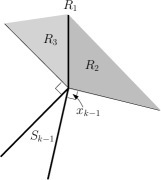
Fig. 3: The cone $C_{S_{k-1}}^{O}\left(\mathbf{x}_{k-1}\right)=R_{1}\cup R_{2}\cup R_{3}$

Theorem 7 can be used to find states on the boundary $S_{k}$, but gives no guarantee of finding all states on the boundary of $S_{k}$. In order to state results directed towards this goal, we need some more definitions. The cone $C_{S_{k-1}}^{O}\left(\mathbf{x}_{k-1}\right)$ associated with any given $\mathbf{x}_{k-1}\in\partial S_{k-1}$ can be partitioned into three disjoint cones:

$$R_{1} =R_{1}\left(\mathbf{x}_{k-1}\right):=C_{S_{k-1}}^{O}\left(\mathbf{x}_{k-1}\right)\cap\left\{\mathbf{x}_{k-1}^{\ast}:\left(\mathbf{x}_{k-1}^{\ast}\right)_{1}=0\right\}$$

$$R_{2} =R_{2}\left(\mathbf{x}_{k-1}\right):=C_{S_{k-1}}^{O}\left(\mathbf{x}_{k-1}\right)\cap\left\{\mathbf{x}_{k-1}^{\ast}:\left(\mathbf{x}_{k-1}^{\ast}\right)_{1}>0\right\}$$

$$R_{3} =R_{3}\left(\mathbf{x}_{k-1}\right):=C_{S_{k-1}}^{O}\left(\mathbf{x}_{k-1}\right)\cap\left\{\mathbf{x}_{k-1}^{\ast}:\left(\mathbf{x}_{k-1}^{\ast}\right)_{1}<0\right\}.$$

At least one of the $R_{i}$ is non-empty. See Fig. 3. One of the $R_{i}$ is selected according to the following rule.

$$R=R\left(\mathbf{x}_{k-1}\right):=\left\{\begin{array}[c]{l}R_{1}\text{ if }R_{1}\neq\emptyset\\ R_{2}\text{ if }R_{1}=\emptyset\text{ and }R_{2}\neq\emptyset\\ R_{3}\text{ if }R_{1}=\emptyset\text{ and }R_{3}\neq\emptyset\text{.}\end{array}\right.$$

This Definition makes sense because, if $R_{1}$ is empty, then precisely one of $R_{2}$ and $R_{3}$ must be non-empty.

Given $\mathbf{x}_{k-1}\in\partial S_{k-1}$, any vector $\mathbf{x}_{k-1}^{\ast}\in R\left(\mathbf{x}_{k-1}\right)$, and $z_{k}$, we define the sets $T$ and $X$.

Definition 8.

$$T\left(\mathbf{x}_{k-1},\mathbf{x}_{k-1}^{\ast},z_{k}\right) :=\left\{\begin{array}[c]{c}\left(\mathbf{x}_{k},\mathbf{x}_{k}^{\ast}\right)=\left(A\mathbf{x}_{k-1}+Bq_{1},A^{\ast}\mathbf{x}_{k-1}^{\ast}+B^{\ast}q_{4}\right)\text{{ }satisfying}\\ \mathbf{x}_{k}^{\ast}\neq\mathbf{0}\text{ and }\mathbf{q}\in M\left(C\mathbf{x}_{k-1},\left(\mathbf{x}_{k-1}^{\ast}\right)_{1},z_{k}\right)\text{.}\end{array}\right\}$$

$$\text{and }X =X\left(T\right):=\left\{\mathbf{x}_{k}:\left(\mathbf{x}_{k},\mathbf{x}_{k}^{\ast}\right)\in T\right\}\text{.}$$

The set $T=T\left(\mathbf{x}_{k-1},\mathbf{x}_{k-1}^{\ast},z_{k}\right)$ can be empty. A useful observation is that although $T$ depends on the choice of $\mathbf{x}_{k-1}^{\ast}\in R$, $X$ does not.

Proposition 9.

For any $\mathbf{x}_{k-1}\in\partial S_{k-1}$ and any $z_{k}$, the set $X\left(T\right)$ does not depend on the choice of $\mathbf{x}_{k-1}^{\ast}\in R\left(\mathbf{x}_{k-1}\right).$

Proof.

Precisely one of $R=R_{1},$ $R=R_{2}$ or $R=R_{3}$ must hold. We show details for the case $R=R_{2}.$ Select any $\mathbf{\bar{x}}_{k-1}^{\ast}\in R_{2}.$ The key observation is that, for any $\mathbf{q}\in M\left(C\mathbf{x}_{k-1},\left(\mathbf{\bar{x}}_{k-1}^{\ast}\right)_{1},z_{k}\right)$, it is only the signs of $q_{3}(=v^{\ast})$ and $q_{4}(=y^{\ast})$ that restrict $q_{1}(=v)$ and $q_{2}(=y)$; that is, for the nine constraint conditions in (33), (34) and Definition 6, the magnitudes of $v^{\ast}$ and $y^{\ast}$ do not constrain $v$ or $y$. But the possible signs of $v^{\ast}$ and $y^{\ast}$ satisfying $d_{m+1}v^{\ast}+n_{m+1}y^{\ast}=-\left(\mathbf{x}_{k-1}^{\ast}\right)_{1}$ are the same for all $\mathbf{x}_{k-1}^{\ast}\in R_{2}$, because $\left(\mathbf{x}_{k-1}^{\ast}\right)_{1}>0$ for all $\mathbf{x}_{k-1}^{\ast}\in R_{2}$. Thus $\left(A\mathbf{x}_{k-1}+Bq_{1},A^{\ast}\mathbf{\bar{x}}_{k-1}^{\ast}+B^{\ast}q_{4}\right)\in T\left(\mathbf{x}_{k-1},\mathbf{\bar{x}}_{k-1}^{\ast},z_{k}\right)$ implies $\left(A\mathbf{x}_{k-1}+Bq_{1},A^{\ast}\mathbf{x}_{k-1}^{\ast}+B^{\ast}q_{4}\right)\in T\left(\mathbf{x}_{k-1},\mathbf{x}_{k-1}^{\ast},z_{k}\right)$ for all $\mathbf{x}_{k-1}^{\ast}\in R_{2}$. The same argument applies for the case $R=R_{3}$, and the case $R=R_{1}$ is similar. ∎

In light of this result, we write $X=X\left(\mathbf{x}_{k-1},z_{k}\right)$.

The main results of the paper are now presented. The ultimate aim is to construct $S_{k}$, and this is achieved when the vertices of $S_{k}$ are known. The following two Theorems provide the basis of a recursive procedure for determining $\partial S_{k}$ from $\partial S_{k-1}$. Theorem 10 follows from Theorem 7 and is proved in Section 6. Theorem 11, which is proved in Section 8, guarantees that vertices of $S_{k}$ have at least one precursor on the boundary of $S_{k-1}$, and shows how any such precursor $\mathbf{x}_{k-1}$, and any $\mathbf{x}_{k-1}^{\ast}\in R\left(\mathbf{x}_{k-1}\right)$, are propagated.

Theorem 10.

Suppose $\mathbf{x}_{k-1}\in\partial S_{k-1}$. If $\mathbf{x}_{k}\in X\left(\mathbf{x}_{k-1},z_{k}\right)$ then $\mathbf{x}_{k}$ is a successor to $\mathbf{x}_{k-1}$ and $\mathbf{x}_{k}\in\partial S_{k}$.

Theorem 11.

Let $\mathbf{x}_{k}$ be a vertex of $S_{k}$. Then there exists $\mathbf{x}_{k-1}\in\partial S_{k-1}$ such that $\mathbf{x}_{k}\in X\left(\mathbf{x}_{k-1},z_{k}\right)$. Furthermore, for all $\mathbf{x}_{k-1}^{\ast}\in R\left(\mathbf{x}_{k-1}\right)$, there holds $\left(\mathbf{x}_{k},\mathbf{x}_{k}^{\ast}\right)\in T\left(\mathbf{x}_{k-1},\mathbf{x}_{k-1}^{\ast},z_{k}\right)$, where $\mathbf{x}_{k}^{\ast}\in C_{S_{k}}^{O}\left(\mathbf{x}_{k}\right)$.

See Fig. 4 for a graphical illustration of finding $M\left(C\mathbf{x}_{k-1},\left(\mathbf{x}_{k-1}^{\ast}\right)_{1},z_{k}\right)$ and $T$. It depicts an Example where $\left(\mathbf{x}_{k-1}^{\ast}\right)_{1}<0$ for all $\mathbf{x}_{k-1}^{\ast}\in C_{S_{k-1}}^{O}\left(\mathbf{x}_{k-1}\right),$ so $R_{1}$ and $R_{2}$ are empty, and $R=R_{3}.$ For this Example $T$ contains the singleton element $\left(A\mathbf{x}_{k-1}+B,A^{\ast}\mathbf{x}_{k-1}^{\ast}\right)$ and $X=\left\{A\mathbf{x}_{k-1}+B\right\}.$ By Theorem 10, if $\mathbf{x}_{k-1}\in\partial S_{k-1}$ then $\mathbf{x}_{k}=A\mathbf{x}_{k-1}+B\in\partial S_{k}$.

Determining the set $M$ does not become any more computationally demanding as $m$ increases. For any $m$ it involves simply finding intersections of straight lines in the plane and checking alignment.

The sets $M$ and $T$ are fundamental. Their description is aided by some notation for points and lines in the plane.

Notation 12.

Associated with any state $\mathbf{x}_{k-1}\in S_{k-1}$ there is the line $y-n_{1}v=C\mathbf{x}_{k-1}$ in the $(y,v)$ plane, denoted $L(\mathbf{x}_{k-1}).$ Denote by $Q$ the set of points on or inside the square with vertices $(1+z_{k},1),(1+z_{k},-1),(-1+z_{k},-1)$ and $(-1+z_{k},1)$.

Not every $\mathbf{x}_{k-1}\in S_{k-1}$ has a successor. Although determining successors $\mathbf{x}_{k}$ on the boundary of $S_{k}$ is the ultimate goal, it is useful to first dispose of the simpler question of determining when $\mathbf{x}_{k-1}\in S_{k-1}$ has a successor anywhere in $S_{k}$.

Proposition 13.

The state $\mathbf{x}_{k-1}\in S_{k-1}$ has a successor $\mathbf{x}_{k}\in S_{k}$ if and only if

$$\left|C\mathbf{x}_{k-1}-z_{k}\right|\leq\left|n_{1}\right|+1.$$

Furthermore, the set of all successors to $\mathbf{x}_{k-1}$ is

$$\left\{\mathbf{x}_{k}:\mathbf{x}_{k}=A\mathbf{x}_{k-1}+Bv,\text{ }(y,v)\in Q\cap L\left(\mathbf{x}_{k-1}\right)\right\}.$$

Proof.

By Definition 1, $\mathbf{x}_{k-1}$ has a successor if and only if scalars $v$ and $y$ exist for which $\left|v\right|\leq 1,$ $\left|y-z_{k}\right|\leq 1$ and $y=C\mathbf{x}_{k-1}+n_{1}v,$ in which case the successor is $\mathbf{x}_{k}=A\mathbf{x}_{k-1}+Bv.$ By elementary geometry of the plane such scalars $v$ and $y$ exist if and only if the line $L\left(\mathbf{x}_{k-1}\right)$ intersects $Q,$ and the Proposition statements follow easily. ∎

The proof of the next Proposition is similar.

Proposition 14.

For any $\mathbf{x}_{k-1}\in\partial S_{k-1}$, and any $\mathbf{x}_{k-1}^{\ast}\in C_{S_{k-1}}^{O}\left(\mathbf{x}_{k-1}\right)$, the sets
$M\left(C\mathbf{x}_{k-1},\left(\mathbf{x}_{k-1}^{\ast}\right)_{1},z_{k}\right)$, $T$ and $X$ are empty if $\left|C\mathbf{x}_{k-1}-z_{k}\right|>\left|n_{1}\right|+1.$

The following two Propositions follow easily from the obvious fact that the line $L\left(\mathbf{x}_{k-1}\right)$ can intersect the boundary of $Q$ at most twice. Let $\mathbf{x}_{k-1}\in\partial S_{k-1}$.

Proposition 15.

If $C_{S_{k-1}}^{O}\left(\mathbf{x}_{k-1}\right)$ is such that $R_{1}=\emptyset$ then the possible values of $\operatorname*{card}\left(X\left(\mathbf{x}_{k-1},z_{k}\right)\right)$ are $0,1$ and $2.$

Proposition 16.

If $C_{S_{k-1}}^{O}\left(\mathbf{x}_{k-1}\right)$ is such that $R_{1}\neq\emptyset$ then the set $X\left(\mathbf{x}_{k-1},z_{k}\right)$ is either empty, contains one element, or is the one-dimensional line segment
$\left\{\mathbf{x}_{k}:\mathbf{x}_{k}=A\mathbf{x}_{k-1}+Bv,\text{ }v\in[v_{\min},v_{\max}]\right\}$ where $v_{\min}$ and $v_{\max}$ are the minimum and maximum values of $v$ for which the line $L\left(\mathbf{x}_{k-1}\right)$ intersects the sides of $Q.$

To proceed further we need duality. The proofs of the Theorems in this Section are based on the duality existing between programs constructed from the estimator and regulator systems.

Fig. 4: For this measurement $z_{k},$ the location of the square implies that the unique element in $M\left(C\mathbf{x}_{k-1},\left(\mathbf{x}_{k-1}^{\ast}\right)_{1},z_{k}\right)$ is $\left(1,n_{1}+C\mathbf{x}_{k-1},\frac{-\left(\mathbf{x}_{k-1}^{\ast}\right)_{1}}{d_{m+1}},0\right)$.

4 The estimator program $\mathcal{E}_{z_{1:k}}(\mathbf{x}^{\ast})$

From now on we will always assume $k\geq 2m$ and $S_{k}\neq\emptyset$. The optimization problem we construct is based on the support function for the set $S_{k}$. Since $S_{k}$ is compact its support function is $h_{S_{k}}(\mathbf{x}^{\ast})=\max_{\mathbf{x}\in S_{k}}\left\langle\mathbf{x}^{\ast},\mathbf{x}\right\rangle$, and the hyperplane $\left\{\mathbf{x}:\left\langle\mathbf{x}^{\ast},\mathbf{x}\right\rangle=h_{S_{k}}(\mathbf{x}^{\ast})\right\}$ in the direction $\mathbf{x}^{\ast}$ supports $S_{k}$ at $\mathbf{x}.$ For any $\mathbf{x}^{\ast}\in\mathbb{R}^{m},$ define the estimator program

$$\mathcal{E}_{z_{1:k}}(\mathbf{x}^{\ast}):\text{ \ \ }\max\limits_{\mathbf{x}\in S_{k}}\left\langle\mathbf{x}^{\ast},\mathbf{x}\right\rangle.$$

It has optimal value $h_{S_{k}}(\mathbf{x}^{\ast}).$ The notation $\mathcal{E}_{z_{1:k}}(\mathbf{\cdot})$ will be used to denote the estimator program when $\mathbf{x}^{\ast}$ is not important or not specified.

The following Proposition follows directly from the definitions.

Proposition 17.

For any $\mathbf{x}\in S_{k}$ and any $\mathbf{x}^{\ast}\in\mathbb{R}^{m},$ there holds

$$\mathbf{x}\in\arg\max\mathcal{E}_{z_{1:k}}(\mathbf{x}^{\ast})\Leftrightarrow h_{S_{k}}(\mathbf{x}^{\ast})=\left\langle\mathbf{x}^{\ast},\mathbf{x}\right\rangle.$$

Furthermore, for any $\mathbf{x}\in\partial S_{k}$ and $\mathbf{0\neq x}^{\ast}\in\mathbb{R}^{m}$ there holds

$$\mathbf{x}\in\arg\max\mathcal{E}_{z_{1:k}}(\mathbf{x}^{\ast})\Leftrightarrow\mathbf{x}^{\ast}\in C_{S_{k}}^{O}(\mathbf{x}).$$

If $S_{k}$ is non-empty and $\mathbf{x}^{\ast}\neq\mathbf{0}$ then optimizing $\mathbf{x}$ must be on the boundary of $S_{k}$, and $\arg\max\mathcal{E}_{z_{1:k}}(\mathbf{x}_{k}^{\ast})$ is a non-empty subset of $\partial S_{k}.$ Any point in $\partial S_{k}$ will belong to $\arg\max\mathcal{E}_{z_{1:k}}(\mathbf{x}^{\ast})$ for some $\mathbf{x}^{\ast}\neq\mathbf{0}$. All of these statements are simple consequences of $S_{k}$ being convex and compact. Some elementary properties relating optimal solutions to the program $\mathcal{E}_{z_{1:k}}(\mathbf{x}^{\ast})$ with geometry of the polytope $S_{k}$ are collected in the next Proposition.

Proposition 18.

Suppose $S_{k}$ is non-empty. Then
1) if $\mathbf{x}\in\partial S_{k}$ and $\mathbf{x}^{\ast}\neq\mathbf{0}$ is the direction of any hyperplane supporting $S_{k}$ at $\mathbf{x}$, then $\mathbf{x}\in\arg\max\mathcal{E}_{z_{1:k}}(\mathbf{x}^{\ast})$;
2) if $\mathbf{x}\in\partial S_{k}$ then there exists $\mathbf{x}^{\ast}\neq\mathbf{0}$ for which $\mathbf{x}\in\arg\max\mathcal{E}_{z_{1:k}}(\mathbf{x}^{\ast})$;
3) if $\mathbf{x}\in\arg\max\mathcal{E}_{z_{1:k}}(\mathbf{x}^{\ast})$ and $\mathbf{x}^{\ast}\neq\mathbf{0}$, then $\mathbf{x}^{\ast}$ is the direction of a hyperplane supporting $S_{k}$ at $\mathbf{x}$;
4) if $\mathbf{x}\in\arg\max\mathcal{E}_{z_{1:k}}(\mathbf{x}^{\ast})$ and $\mathbf{x}\in\operatorname*{int}S_{k}$, then $\mathbf{x}^{\ast}=\mathbf{0}$; and
5) $\arg\max$ $\mathcal{E}_{z_{1:k}}(\mathbf{0})=S_{k}$.

A program almost identical to $\mathcal{E}_{z_{1:k}}(\mathbf{x}^{\ast})$, denoted $\mathcal{E}_{z_{1:k}}^{\prime}(\mathbf{x}^{\ast})$, is introduced for notational clarity. By (29) $\mathcal{E}_{z_{1:k}}(\mathbf{x}^{\ast})$ can be equivalently expressed as

$$\begin{array}[c]{c}\mathcal{E}_{z_{1:k}}^{\prime}(\mathbf{x}^{\ast}):\text{ \ \ }\max\limits_{y_{1:k},v_{1:k}}\left\langle\mathbf{x}^{\ast},\mathbf{x}\right\rangle\\ \text{subject to }\\ \left\|y_{1:k}-z_{1:k}\right\|_{\infty}\leq 1,\text{ }\left\|v_{1:k}\right\|_{\infty}\leq 1\text{ and}\\ \left[\begin{array}[c]{cccc}D_{L}&&&\\ D_{U}&D_{L}&&\\ &\ddots&\ddots&\\ &&D_{U}&D_{L}\\ &&&D_{U}\end{array}\right]\left[\begin{array}[c]{c}y_{1}\\ \vdots\\ y_{k}\end{array}\right]-\\ \left[\begin{array}[c]{cccc}N_{L}&&&\\ N_{U}&N_{L}&&\\ &\ddots&\ddots&\\ &&N_{U}&N_{L}\\ &&&N_{U}\end{array}\right]\left[\begin{array}[c]{c}v_{1}\\ \vdots\\ v_{k}\end{array}\right]=\left[\begin{array}[c]{c}B_{T}\mathbf{x}_{0}\\ 0\\ \vdots\\ 0\\ -B_{T}\mathbf{x}\end{array}\right]\begin{array}[c]{c}\text{fixed}\\ \\ \\ \\ \text{free}\end{array}\end{array}.$$

By (8) the final state $\mathbf{x}$ satisfies $\mathbf{x=x}_{k}\left(y_{1:k},v_{1:k}\right)$. See Fig. 5. The decision variables for the program $\mathcal{E}_{z_{1:k}}^{\prime}(\mathbf{x}^{\ast})$ are the outputs and inputs of the estimation system up to time $k.$ From now on we put $(\mathbf{y},\mathbf{v}):=\left(y_{1:k},v_{1:k}\right),$ and later $(\mathbf{y}^{\ast},\mathbf{v}^{\ast}):=\left(y_{1:k}^{\ast},v_{1:k}^{\ast}\right)$. The relationship between estimator signals $(\mathbf{y},\mathbf{v})$ and states $\mathbf{x}\in\partial S_{k}$ occurring as optimizing decision variables in the programs $\mathcal{E}_{z_{1:k}}(\mathbf{x}^{\ast})$ and $\mathcal{E}_{z_{1:k}}^{\prime}(\mathbf{x}^{\ast})$ is summarized in the following Proposition.

Proposition 19.

1) For all $\mathbf{x}\in\partial S_{k}$, and for all $\mathbf{x}^{\ast}\in C_{S_{k}}^{O}(\mathbf{x}),$ there exists $\left(\mathbf{y},\mathbf{v}\right)$ $\in\arg\max\mathcal{E}_{z_{1:k}}^{\prime}(\mathbf{x}^{\ast})$ for which $\mathbf{x}=\mathbf{x}_{k}\left(\mathbf{y},\mathbf{v}\right)$.
2) Suppose $\mathbf{x}^{\ast}\in\mathbb{R}^{m}$ and $(\mathbf{y},\mathbf{v})\in\mathbb{R}^{k}\times\mathbb{R}^{k}$. Then $(\mathbf{y},\mathbf{v})\in\arg\max\mathcal{E}_{z_{1:k}}^{\prime}(\mathbf{x}^{\ast})$ if and only if $\mathbf{x}_{k}(\mathbf{y},\mathbf{v})\in\arg\max\mathcal{E}_{z_{1:k}}(\mathbf{x}^{\ast})$.

Note also that the origin may or may not be in $S_{k}$. If $S_{k}$ does not contain the origin then there will exist $\mathbf{x}^{\ast}$ for which $h_{S_{k}}\left(\mathbf{x}^{\ast}\right)<0.$

5 The regulator program $\mathcal{R}_{z_{1:k}}(\mathbf{x}^{\ast})$

We would like to use a dynamic programming style argument to determine all optimal solutions to the program $\mathcal{E}_{z_{1:k}}(\mathbf{x}_{k}^{\ast})$ recursively from a known optimal solution to $\mathcal{E}_{z_{1:k-1}}(\mathbf{x}_{k-1}^{\ast}),$ where $\mathbf{x}_{k}^{\ast}$ is determined recursively from $\mathbf{x}_{k-1}^{\ast}.$ Such a recursion would yield point(s) on the boundary of the feasible set for $\mathcal{E}_{z_{1:k}}(\mathbf{x}_{k}^{\ast}),$ the desired points on the boundary of $S_{k}.$ However, the cost function for the program $\mathcal{E}_{z_{1:k}}(\mathbf{x}_{k}^{\ast})$ is not in a form suitable for application of dynamic programming. We make use of a program with a dual pairing to $\mathcal{E}_{z_{1:k}}(\mathbf{x}_{k}^{\ast}),$ termed the regulator program, and denoted $\mathcal{R}_{z_{1:k}}(\mathbf{x}_{k}^{\ast}),$ for which the cost function is of a suitable form. Although a straightforward application of dynamic programming to $\mathcal{R}_{z_{1:k}}(\mathbf{x}_{k}^{\ast})$ by itself does not yield a computationally tractable recursion, we show that linking the optimal solutions to $\mathcal{R}_{z_{1:k}}(\mathbf{x}_{k}^{\ast})$ and $\mathcal{E}_{z_{1:k}}(\mathbf{x}_{k}^{\ast})$ through alignment (complementary slackness) conditions, in conjunction with the use of dynamic programming, does yield the desired recursion.

The duality between $\mathcal{R}_{z_{1:k}}(\mathbf{x}^{\ast})$ and $\mathcal{E}_{z_{1:k}}(\mathbf{x}^{\ast})$ will now be interpreted in the structural form required to carry through this plan. The regulator program is defined as:

$$\begin{array}[c]{c}\mathcal{R}_{z_{1:k}}(\mathbf{x}^{\ast}):\text{ \ \ }\min\limits_{\mathbf{y}^{\ast},\mathbf{v}^{\ast}}\left\{\left\|\mathbf{y}^{\ast}\right\|_{1}+\left\|\mathbf{v}^{\ast}\right\|_{1}+\left\langle y_{1:k}^{\ast},z_{1:k}\right\rangle+\left\langle\mathbf{x}_{0}^{\ast},\mathbf{x}_{0}\right\rangle\right\}\\ \text{subject to }\\ \left[\begin{array}[c]{cccc}N_{U}^{T}&&&\\ N_{L}^{T}&N_{U}^{T}&&\\ &\ddots&\ddots&\\ &&N_{L}^{T}&N_{U}^{T}\\ &&&N_{L}^{T}\end{array}\right]\left[\begin{array}[c]{c}y_{1}^{\ast}\\ \vdots\\ y_{k}^{\ast}\end{array}\right]+\\ \left[\begin{array}[c]{cccc}D_{U}^{T}&&&\\ D_{L}^{T}&D_{U}^{T}&&\\ &\ddots&\ddots&\\ &&D_{L}^{T}&D_{U}^{T}\\ &&&D_{L}^{T}\end{array}\right]\left[\begin{array}[c]{c}v_{1}^{\ast}\\ \vdots\\ v_{k}^{\ast}\end{array}\right]=\left[\begin{array}[c]{c}-\mathbf{x}_{0}^{\ast}\\ 0\\ \vdots\\ 0\\ \mathbf{x}^{\ast}\end{array}\right]\begin{array}[c]{c}\text{free}\\ \\ \\ \\ \text{fixed}\end{array}\end{array}$$

The decision variables are the inputs and outputs of the regulator system up to time $k$ described in Section 2.3. See Fig. 6. If the measurements are all zero, $\mathbf{x}_{0}=\mathbf{0}$ and $k\rightarrow\infty$, then $\mathcal{R}_{z_{1:k}}(\mathbf{x}^{\ast})$ has an interpretation as a time-reversed deterministic $l_{1}$-norm regulator problem, where the input and output signals are made as small as possible and driven asymptotically to zero.

A formal statement of the duality existing between $\mathcal{E}_{z_{1:k}}^{\prime}(\mathbf{x}^{\ast})$ and $\mathcal{R}_{z_{1:k}}(\mathbf{x}^{\ast})$ is now stated.

Proposition 20.

Suppose the set $S_{k}$ is non-empty. Then the optimal values of $\mathcal{E}_{z_{1:k}}^{\prime}(\mathbf{x}^{\ast})$ and $\mathcal{R}_{z_{1:k}}(\mathbf{x}^{\ast})$ are finite and equal. Furthermore, if $(\mathbf{y},\mathbf{v})$ and $(\mathbf{y}^{\ast},\mathbf{v}^{\ast})$ are feasible for $\mathcal{E}_{z_{1:k}}^{{}^{\prime}}(\mathbf{x}^{\ast})$ and $\mathcal{R}_{z_{1:k}}(\mathbf{x}^{\ast}),$ respectively, then a necessary and sufficient condition that they both be optimal is that they be aligned.

Proof.

The proof in outline follows standard linear programming arguments. The Gohberg-Semencul formula (2) is also required. Details are in the Appendix. ∎

Remark 21.

For the program $\mathcal{R}_{z_{1:k}}(\mathbf{x}^{\ast})$ the initial state is free, and the terminal state is fixed, at $\mathbf{x}^{\ast}$. For the program $\mathcal{E}_{z_{1:k}}^{\prime}(\mathbf{x}^{\ast})$ the initial state is fixed, at $\mathbf{x}_{0}$, and the terminal state is free.

Fig. 5: The program $\mathcal{E}_{z_{1:k}}(\mathbf{x}_{k}^{\ast}).$ If $\mathbf{x}_{k}^{\ast}\neq\mathbf{0}$ then optimizing $\mathbf{x}_{k}$ are points on the boundary of $S_{k}.$

Fig. 6: The program $\mathcal{R}_{z_{1:k}}(\mathbf{x}_{k}^{\ast})$

6 Combined recursion in the estimator and regulator programs

Our goal is determine when and how a state $\mathbf{x}_{k-1}\in\partial S_{k-1}$ is propagated to a successor $\mathbf{x}_{k}\in\partial S_{k}$. Now $\mathbf{x}_{k-1}$ has at least one associated worst-case disturbance $v_{1:k-1},$ and if $\left\langle\mathbf{x}_{k-1}^{\ast},\mathbf{x}_{k-1}\right\rangle=h_{S_{k-1}}(\mathbf{x}_{k-1}^{\ast})$ then $\left(y_{1:k-1},v_{1:k-1}\right)\in\arg\max\mathcal{E}_{z_{1:k-1}}^{\prime}(\mathbf{x}_{k-1}^{\ast})$ where, by (32), $y_{1:k-1}$ is uniquely determined by $v_{1:k-1},$ $z_{1:k-1}$ and $\mathbf{x}_{0}.$ By Proposition 20, for all such $\left(y_{1:k-1},v_{1:k-1}\right)\in\arg\max\mathcal{E}_{z_{1:k-1}}^{\prime}(\mathbf{x}_{k-1}^{\ast}),$ there exists $\left(y_{1:k-1}^{\ast},v_{1:k-1}^{\ast}\right)\in\arg\min$$\mathcal{R}_{z_{1:k-1}}(\mathbf{x}_{k-1}^{\ast}),$ and $\left(y_{1:k-1}^{\ast},v_{1:k-1}^{\ast}\right)$ is aligned with $\left(y_{1:k-1},v_{1:k-1}\right).$ The next Proposition yields useful extensions to $\left(y_{1:k-1},v_{1:k-1}\right)$ and $\left(y_{1:k-1}^{\ast},v_{1:k-1}^{\ast}\right)$.

Proposition 22.

Suppose $\mathbf{x}_{k-1}$ and $\mathbf{x}_{k-1}^{\ast}$ satisfying $\left\langle\mathbf{x}_{k-1},\mathbf{x}_{k-1}^{\ast}\right\rangle=h_{S_{k-1}}(\mathbf{x}_{k-1}^{\ast})$ are given. Select any $\left(y_{1:k-1},v_{1:k-1}\right)\in\arg\max\mathcal{E}_{z_{1:k-1}}^{\prime}(\mathbf{x}_{k-1}^{\ast}),$ and any $\left(y_{1:k-1}^{\ast},v_{1:k-1}^{\ast}\right)\in\arg\min$$\mathcal{R}_{z_{1:k-1}}(\mathbf{x}_{k-1}^{\ast}).$ Then $\left(y_{1:k},v_{1:k}\right)\in\arg\max\mathcal{E}_{z_{1:k}}^{\prime}(A^{\ast}\mathbf{x}_{k-1}^{\ast}+B^{\ast}y_{k}^{\ast})$ and $\left(y_{1:k}^{\ast},v_{1:k}^{\ast}\right)\in\arg\min$$\mathcal{R}_{z_{1:k}}(A^{\ast}\mathbf{x}_{k-1}^{\ast}+B^{\ast}y_{k}^{\ast})$ if $\left(v_{k},y_{k},v_{k}^{\ast},y_{k}^{\ast}\right)\in\linebreak M\left(C\mathbf{x}_{k-1},\left(\mathbf{x}_{k-1}^{\ast}\right)_{1},z_{k}\right)$.

Proof.

First note that, from the discussion above, there does exist $\left(y_{1:k-1},v_{1:k-1}\right)\in\arg\max\mathcal{E}_{z_{1:k-1}}(\mathbf{x}_{k-1}^{\ast})$ and $\left(y_{1:k-1}^{\ast},v_{1:k-1}^{\ast}\right)\in\arg\min$$\mathcal{R}_{z_{1:k-1}}(\mathbf{x}_{k-1}^{\ast}),$ and that $\left(y_{1:k-1}^{\ast},v_{1:k-1}^{\ast}\right)$ is aligned with $\left(y_{1:k-1},v_{1:k-1}\right)$.

Suppose $\left(v_{k},y_{k},v_{k}^{\ast},y_{k}^{\ast}\right)\in M\left(C\mathbf{x}_{k-1},\left(\mathbf{x}_{k-1}^{\ast}\right)_{1},z_{k}\right)$. It follows from the state space representation of the estimator system (6) that, since $y_{k}$ satisfies $y_{k}-n_{1}v_{k}=C\mathbf{x}_{k-1}$ (that is $y_{k}=C\mathbf{x}_{k-1}+D_{1}v_{k}$), then $\mathbf{x}_{k}:=A\mathbf{x}_{k-1}+Bv_{k}$ satisfies $\mathbf{x}_{k}=\mathbf{x}_{k}(\mathbf{y},\mathbf{v}),$ where $(\mathbf{y},\mathbf{v})=\left(y_{1:k},v_{1:k}\right)$ satisfies the matrix contraint equations for $\mathcal{E}_{z_{1:k}}(\mathbf{\cdot}).$ Since also $\left|v_{k}\right|\leq 1$ and $\left|y_{k}-z_{k}\right|\leq 1$ hold it follows that $(\mathbf{y},\mathbf{v})$ is feasible for $\mathcal{E}_{z_{1:k}}(\mathbf{\cdot})$.

From the regulator system representation (10), (11), satisfaction of $v_{k}^{\ast}=C^{\ast}\mathbf{x}_{k-1}^{\ast}+D_{1}^{\ast}y_{k}^{\ast}$ by $y_{k}^{\ast}$ and $v_{k}^{\ast}$ implies $(\mathbf{y}^{\ast},\mathbf{v}^{\ast})=\left(y_{1:k}^{\ast},v_{1:k}^{\ast}\right)$ is feasible for $\mathcal{R}_{z_{1:k}}(\mathbf{x}_{k}^{\ast}),$ where $\mathbf{x}_{k}^{\ast}:=A^{\ast}\mathbf{x}_{k-1}^{\ast}+B^{\ast}y_{k}^{\ast}.$ Since $\left(y_{1:k-1},v_{1:k-1}\right)$ is aligned with $\left(y_{1:k-1}^{\ast},v_{1:k-1}^{\ast}\right),$ and $\left(v_{k},y_{k},v_{k}^{\ast},y_{k}^{\ast}\right)\in M\left(C\mathbf{x}_{k-1},\left(\mathbf{x}_{k-1}^{\ast}\right)_{1},z_{k}\right)\Rightarrow\left(y_{k},v_{k}\right)$ is aligned at time $k$ with $\left(y_{k}^{\ast},v_{k}^{\ast}\right),$ we have $(\mathbf{y},\mathbf{v})$ is aligned with $(\mathbf{y}^{\ast},\mathbf{v}^{\ast}).$ We have shown that $(\mathbf{y},\mathbf{v})$ and $(\mathbf{y}^{\ast},\mathbf{v}^{\ast})$ are feasible for $\mathcal{E}_{z_{1:k}}(\mathbf{x}_{k}^{\ast})$ and $\mathcal{R}_{z_{1:k}}(\mathbf{x}_{k}^{\ast})$, and that they are aligned. By Proposition 20, $(\mathbf{y},\mathbf{v})$ and $(\mathbf{y}^{\ast},\mathbf{v}^{\ast})$ are optimal for $\mathcal{E}_{z_{1:k}}(\mathbf{x}_{k}^{\ast})$ and $\mathcal{R}_{z_{1:k}}(\mathbf{x}_{k}^{\ast})$, respectively. ∎

As an immediate application of Proposition 22 we now prove Theorem 7.

Proof of Theorem 7

Suppose $\mathbf{x}_{k-1}\in\partial S_{k-1}$, $\mathbf{x}_{k-1}^{\ast}\in C_{S_{k-1}}^{O}(\mathbf{x}_{k-1})$ and $\left(v_{k},y_{k},v_{k}^{\ast},y_{k}^{\ast}\right)\in M\left(C\mathbf{x}_{k-1},\left(\mathbf{x}_{k-1}^{\ast}\right)_{1},z_{k}\right)$. Now $\mathbf{x}_{k-1}^{\ast}\in C_{S_{k-1}}^{O}(\mathbf{x}_{k-1})\Rightarrow\left\langle\mathbf{x}_{k-1}^{\ast},\mathbf{x}_{k-1}\right\rangle=h_{S_{k-1}}(\mathbf{x}_{k-1}^{\ast})$ so, by Proposition 22, for any $\left(y_{1:k-1},v_{1:k-1}\right)\in\arg\max\mathcal{E}_{z_{1:k-1}}(\mathbf{x}_{k-1}^{\ast}),$ and any $\left(y_{1:k-1}^{\ast},v_{1:k-1}^{\ast}\right)\in\arg\min$$\mathcal{R}_{z_{1:k-1}}(\mathbf{x}_{k-1}^{\ast}),$ there holds $\left(y_{1:k},v_{1:k}\right)=:(\mathbf{y},\mathbf{v})\in\arg\max\mathcal{E}_{z_{1:k}}(\mathbf{x}_{k}^{\ast})$ and $\left(y_{1:k}^{\ast},v_{1:k}^{\ast}\right)=:(\mathbf{y}^{\ast},\mathbf{v}^{\ast})\in\arg\min$$\mathcal{R}_{z_{1:k}}(\mathbf{x}_{k}^{\ast})$, where $\mathbf{x}_{k}^{\ast}=A^{\ast}\mathbf{x}_{k-1}^{\ast}+B^{\ast}y_{k}^{\ast}.$ Hence, by the second statement of Proposition 19, $\mathbf{x}_{k}:=\mathbf{x}_{k}(\mathbf{y},\mathbf{v})\in$ $\arg\max\mathcal{E}_{z_{1:k}}(\mathbf{x}_{k}^{\ast}),$ and by (6) $\mathbf{x}_{k}=A\mathbf{x}_{k-1}+Bv_{k}$. By assumption $\mathbf{x}_{k}^{\ast}\neq\mathbf{0}$, so $\mathbf{x}_{k}\in\partial S_{k}$. Then Proposition 17 implies $\mathbf{x}_{k}^{\ast}\in C_{S_{k}}^{O}(\mathbf{x}_{k})$. Finally, $\mathbf{x}_{k}$ being a successor to $\mathbf{x}_{k-1}$ follows from $\left(y_{1:k-1},v_{1:k-1}\right)$ being feasible for $\arg\max\mathcal{E}_{z_{1:k-1}}(\mathbf{x}_{k-1}^{\ast})$, the second Condition of Definition 6 and Proposition 2.

The proof of Theorem 10 follows directly.

Proof of Theorem 10

If $\mathbf{x}_{k}\in X\left(\mathbf{x}_{k-1},z_{k}\right)$ then there exists $\mathbf{x}_{k-1}^{\ast}\in R(\mathbf{x}_{k-1})$ and $\mathbf{q}\in M\left(C\mathbf{x}_{k-1},\left(\mathbf{x}_{k-1}^{\ast}\right)_{1},z_{k}\right)$ such that $\left(\mathbf{x}_{k},\mathbf{x}_{k}^{\ast}\right):=\left(A\mathbf{x}_{k-1}+Bq_{1},A^{\ast}\mathbf{x}_{k-1}^{\ast}+B^{\ast}q_{4}\right)$ and $\mathbf{x}_{k}^{\ast}\neq\mathbf{0}$. Since $\mathbf{x}_{k-1}^{\ast}\in C_{S_{k-1}}^{O}(\mathbf{x}_{k-1})$, by Theorem 7, $\mathbf{x}_{k}\in\partial S_{k}$ and $\mathbf{x}_{k}$ is a successor to $\mathbf{x}_{k-1}$.

From Theorem 10 we have a procedure that is guaranteed to produce states that lie on the boundary of $S_{k}$ when $T$ is non-empty. But not yet addressed is the question: Under what conditions are all successors of $\mathbf{x}_{k-1}\in\partial S_{k-1}$ that lie on the boundary of $S_{k}$ contained in $X(\mathbf{x}_{k-1},z_{k})$? Also, there may be points on the boundary of $S_{k}$ whose precursors are in the interior of $S_{k-1}$. These issues are examined next.

7 Finding precursors of a given $\mathbf{x}_{k}\in\partial S_{k}$

In the previous Section we were given $\mathbf{x}_{k-1}\in\partial S_{k-1}$ and any $\mathbf{x}_{k-1}^{\ast}\in R(\mathbf{x}_{k-1})$, and showed that all states $\mathbf{x}_{k}\in X\left(\mathbf{x}_{k-1},z_{k}\right)$ belong to $\partial S_{k}.$ The question is now turned around: For a given $\mathbf{x}_{k}\in\partial S_{k},$ where are the precursors? To answer this question we need dynamic programming.

7.1 Dynamic programming applied to the programs $\mathcal{E}_{z_{1:k}}(\mathbf{\cdot})$ and $\mathcal{R}_{z_{1:k}}(\mathbf{\cdot})$

Let $k>2m$ be an integer. Recall, from (27), $\mathbf{x}_{k}^{\ast}\left(\mathbf{y}^{\ast},\mathbf{v}^{\ast}\right):=N_{L}^{T}y_{k-m+1:k}^{\ast}+D_{L}^{T}v_{k-m+1:k}^{\ast},$ so $\mathbf{x}_{k-1}^{\ast}\left(\mathbf{y}^{\ast},\mathbf{v}^{\ast}\right)=N_{L}^{T}y_{k-m:k-1}^{\ast}+D_{L}^{T}v_{k-m:k-1}^{\ast}$. Also, from (8), $\mathbf{x}_{k-1}\left(\mathbf{y},\mathbf{v}\right)=B_{T}^{-1}\left[-D_{U}y_{k-m:k-1}+N_{U}v_{k-m:k-1}\right].$

Proposition 23.

For any $\mathbf{x}_{k}^{\ast}\in\mathbb{R}^{m},$ any $\left(\mathbf{y}^{\ast},\mathbf{v}^{\ast}\right)\in\arg\min$$\mathcal{R}_{z_{1:k}}(\mathbf{x}_{k}^{\ast})$ and any $\left(\mathbf{y},\mathbf{v}\right)\in\arg\max\mathcal{E}_{z_{1:k}}^{\prime}(\mathbf{x}_{k}^{\ast}),$ there holds
(i) $\left(y_{1:k-1}^{\ast},v_{1:k-1}^{\ast}\right)\in\arg\min$$\mathcal{R}_{z_{1:k-1}}\left(\mathbf{x}_{k-1}^{\ast}\left(\mathbf{y}^{\ast},\mathbf{v}^{\ast}\right)\right)$,
(ii) $\left(y_{1:k-1},v_{1:k-1}\right)\in\arg\max\mathcal{E}_{z_{1:k-1}}^{\prime}\left(\mathbf{x}_{k-1}^{\ast}\left(\mathbf{y}^{\ast},\mathbf{v}^{\ast}\right)\right)$, and(iii) $\left\langle\mathbf{x}_{k-1}^{\ast}\left(y^{\ast},v^{\ast}\right),\mathbf{x}_{k-1}\left(y,v\right)\right\rangle=h_{S_{k-1}}(\mathbf{x}_{k-1}^{\ast}\left(\mathbf{y}^{\ast},\mathbf{v}^{\ast}\right))$.

Proof.

(i) This follows immediately from the dynamic programming principle of optimality. If $\left(y_{1:k-1}^{\ast},v_{1:k-1}^{\ast}\right)\notin\arg\min$$\mathcal{R}_{z_{1:k-1}}\left(\mathbf{x}_{k-1}^{\ast}\left(\mathbf{y}^{\ast},\mathbf{v}^{\ast}\right)\right)$ then, for any $\left(\bar{y}_{1:k-1}^{\ast},\bar{v}_{1:k-1}^{\ast}\right)\in\arg\min\mathcal{R}_{z_{1:k-1}}(\mathbf{x}_{k-1}^{\ast}\left(\mathbf{y}^{\ast},\mathbf{v}^{\ast}\right)),$ we have $\left((\bar{y}_{1:k-1}^{\ast},y_{k}^{\ast}),(\bar{v}_{1:k-1}^{\ast},v_{k}^{\ast})\right)$ is feasible for $\mathcal{R}_{z_{1:k}}(\mathbf{x}_{k}^{\ast})$ with a lower cost than $\left(\mathbf{y}^{\ast},\mathbf{v}^{\ast}\right)\in\arg\min$$\mathcal{R}_{z_{1:k}}(\mathbf{x}_{k}^{\ast}),$ a contradiction.
(ii) By (i), $\left(y_{1:k-1}^{\ast},v_{1:k-1}^{\ast}\right)\in\arg\min$$\mathcal{R}_{z_{1:k-1}}\left(\mathbf{x}_{k-1}^{\ast}\left(\mathbf{y}^{\ast},\mathbf{v}^{\ast}\right)\right)$, and Theorem 20 applied to $\mathcal{R}_{z_{1:k}}(\mathbf{x}_{k}^{\ast})$ and $\mathcal{E}_{z_{1:k}}^{\prime}(\mathbf{x}_{k}^{\ast})$ implies that $\left(y_{1:k-1},v_{1:k-1}\right)$ is aligned with $\left(y_{1:k-1}^{\ast},v_{1:k-1}^{\ast}\right)$. Since also $\left(y_{1:k-1},v_{1:k-1}\right)$ is feasible for $\mathcal{E}_{z_{1:k-1}}^{\prime}\left(\mathbf{x}_{k-1}^{\ast}\left(\mathbf{y}^{\ast},\mathbf{v}^{\ast}\right)\right)$ Theorem 20 applied to $\mathcal{R}_{z_{1:k-1}}(\mathbf{x}_{k-1}^{\ast})$ and $\mathcal{E}_{z_{1:k-1}}^{\prime}(\mathbf{x}_{k-1}^{\ast})$ gives $\left(y_{1:k-1},v_{1:k-1}\right)\in\arg\max\mathcal{E}_{z_{1:k-1}}^{\prime}\left(\mathbf{x}_{k-1}^{\ast}\left(\mathbf{y}^{\ast},\mathbf{v}^{\ast}\right)\right).$ Furthermore, Proposition 18 applied to $\mathcal{E}_{z_{1:k-1}}\left(\mathbf{x}_{k-1}^{\ast}\left(\mathbf{y}^{\ast},\mathbf{v}^{\ast}\right)\right)$ gives $\mathbf{x}_{k-1}\left(y,v\right)\in\arg\max\mathcal{E}_{z_{1:k-1}}\left(\mathbf{x}_{k-1}^{\ast}\left(\mathbf{y}^{\ast},\mathbf{v}^{\ast}\right)\right)$, implying (iii). ∎

In Proposition 23 a relationship between evolving, connected estimator and regulator states is given. Some extra notation is helpful in such situations. In similar fashion to the use of the terms successor and precursor for estimator states, we make the following definition for regulator states. Different definitions of the word successor in Definitions 1 and 24 should not cause confusion as the Definition 1 is used exclusively for unstarred, estimator variables, and Definition 24 exclusively for starred regulator variables. Recall from (27) the definition $\mathbf{x}_{k-1}^{\ast}(\mathbf{y}^{\ast},\mathbf{v}^{\ast}):=N_{L}^{T}y_{k-m:k-1}^{\ast}+D_{L}^{T}v_{k-m:k-1}^{\ast}$.

Definition 24.

The vector $\mathbf{x}_{k}^{\ast}$ is a successor to the vector $\mathbf{x}_{k-1}^{\ast},$ and $\mathbf{x}_{k-1}^{\ast}$ is a precursor of $\mathbf{x}_{k}^{\ast},$ if there exists $(\mathbf{y}^{\ast},\mathbf{v}^{\ast})\in\arg\min\mathcal{R}_{z_{1:k}}(\mathbf{x}_{k}^{\ast})$ and $\mathbf{x}_{k-1}^{\ast}=\mathbf{x}_{k-1}^{\ast}(\mathbf{y}^{\ast},\mathbf{v}^{\ast}).$

For the case $\mathbf{x}_{k}^{\ast}\neq\mathbf{0}$ Proposition 23 yields the following useful result.

Theorem 25.

Let $\mathbf{x}_{k-1}$ be a precursor of $\mathbf{x}_{k}\in\partial S_{k}$, and let $\mathbf{x}_{k-1}^{\ast}$ be a precursor of $\mathbf{x}_{k}^{\ast}\in C_{S_{k}}^{O}\left(\mathbf{x}_{k}\right)$. Then

$$\text{(i) }\mathbf{x}_{k-1} \in\operatorname*{int}S_{k-1}\Rightarrow\mathbf{x}_{k-1}^{\ast}=\mathbf{0}\text{; and}$$

$$\text{(ii) if }\mathbf{x}_{k-1} \in\partial S_{k-1}\text{ and }\mathbf{x}_{k-1}^{\ast}\neq\mathbf{0}\text{, then }\mathbf{x}_{k-1}^{\ast}\in C_{S_{k-1}}^{O}(\mathbf{x}_{k-1})\text{.}$$

Proof.

Since $\mathbf{x}_{k}$ is a successor to $\mathbf{x}_{k-1}$, by Proposition 2 there exists $\mathbf{y=}y_{1:k}$ and $\mathbf{v=}v_{1:k}$ such that $\left(\mathbf{y},\mathbf{v}\right)$ is feasible for the program $\mathcal{E}_{z_{1:k}}^{\prime}(\mathbf{\cdot})$, $\mathbf{x}_{k}=\mathbf{x}_{k}\left(\mathbf{y},\mathbf{v}\right)$, and $\mathbf{x}_{k-1}=\mathbf{x}_{k-1}\left(\mathbf{y},\mathbf{v}\right)$. By Proposition 23, $\mathbf{x}_{k-1}\in\arg\max\mathcal{E}_{z_{1:k}}(\mathbf{x}_{k-1}^{\ast})$. Then (i) follows from statement 4 of Proposition 18, and (ii) follows from the first statement in Proposition 18 and Proposition 17. ∎

7.2 Precursors of $\mathbf{x}_{k}\in\partial S_{k}$ that lie on the boundary of $S_{k-1}$

This Section is devoted to a proof of Theorem 31, which says that if a state $\mathbf{x}_{k}$ is in a particular subset of the boundary of $S_{k}$, and is a successor to some state $\mathbf{x}_{k-1}$ on the boundary of $S_{k-1}$, then determining $X(\mathbf{x}_{k-1},z_{k})$ suffices to produce $\mathbf{x}_{k}$. Fortunately this subset of the boundary of $S_{k}$ is big enough to include all vertices of $S_{k}$.

Some preliminary results are required. The first concerns direction vectors in $C_{S_{k-1}}^{O}(\mathbf{x}_{k-1})$. A simplifying feature of the results in Theorems 10 and 11 is that only one element of the cone $C_{S_{k-1}}^{O}(\mathbf{x}_{k-1})$ is needed to propagate $\mathbf{x}_{k-1}$ to $\mathbf{x}_{k}$, because the set $X\left(\mathbf{x}_{k-1},z_{k}\right)$ is constructed from only one such element. In our proofs it is often convenient to argue using the set $X^{O}$ defined below; the fact that Theorems 10 and 11 can be stated simply in terms of $X$ depends on Proposition 27 below.

Definition 26.

Given any $\mathbf{x}_{k-1}\in\partial S_{k-1}$, the set $X^{O}\left(\mathbf{x}_{k-1},z_{k}\right)=X^{O}$ is defined as

$$X^{O}:={\displaystyle\bigcup\limits_{\mathbf{x}_{k-1}^{\ast}\in C_{S_{k-1}}^{O}\left(\mathbf{x}_{k-1}\right)}}\left\{\begin{array}[c]{c}\mathbf{x}_{k}:\mathbf{x}_{k}=A\mathbf{x}_{k-1}+Bq_{1},\mathbf{q}\in M\left(C\mathbf{x}_{k-1},\left(\mathbf{x}_{k-1}^{\ast}\right)_{1},z_{k}\right)\\ \text{and }A^{\ast}\mathbf{x}_{k-1}^{\ast}+B^{\ast}q_{4}\neq\mathbf{0}\end{array}\right\}\text{.}$$

From Definition 8 and Proposition 9 we have, for an arbitrarily selected $\mathbf{x}_{k-1}^{\ast}\in R(\mathbf{x}_{k-1})$, that $X=X\left(\mathbf{x}_{k-1},z_{k}\right)$ is given by

$$X=\left\{\mathbf{x}_{k}:\mathbf{x}_{k}=A\mathbf{x}_{k-1}+Bq_{1},\mathbf{q}\in M\left(C\mathbf{x}_{k-1},\left(\mathbf{x}_{k-1}^{\ast}\right)_{1},z_{k}\right),A^{\ast}\mathbf{x}_{k-1}^{\ast}+B^{\ast}q_{4}\neq\mathbf{0}\right\}\text{.}$$

The set $X^{O}$ would appear to be bigger than $X$, so the following Proposition is at first sight surprising.

Proposition 27.

For any $\mathbf{x}_{k-1}\in\partial S_{k-1}$ there holds $X^{O}\left(\mathbf{x}_{k-1},z_{k}\right)=X\left(\mathbf{x}_{k-1},z_{k}\right)$.

Proof.

Obviously $X\subseteq X^{O}$, so the proof is complete if it can be shown that $\mathbf{x}_{k}\in X^{O}\Rightarrow\mathbf{x}_{k}\in X$. We assume $\mathbf{x}_{k}\in X^{O}$ and, for any $\mathbf{x}_{k-1}^{\ast}\in C_{S_{k-1}}^{O}\left(\mathbf{x}_{k-1}\right)$, case split the three possibilities $\mathbf{x}_{k-1}^{\ast}\in R_{i}$. In each case it is shown that $\mathbf{x}_{k}\in X$.
Case (i). If $\mathbf{x}_{k-1}^{\ast}\in R_{1}$, then $R\left(x_{k-1}\right)=R_{1}\neq\emptyset$, and $\mathbf{x}_{k-1}^{\ast}\in R(\mathbf{x}_{k-1})\Rightarrow\mathbf{x}_{k}\in X.$
Case (ii). Now suppose $\mathbf{x}_{k-1}^{\ast}\in R_{2}$. If $R_{1}$ is empty then $\mathbf{x}_{k-1}^{\ast}\in R_{2}=R(\mathbf{x}_{k-1})\Rightarrow\mathbf{x}_{k}\in X$. So assume $R=R_{1}\neq\emptyset$. Select any $\mathbf{\bar{x}}_{k-1}^{\ast}\in R(\mathbf{x}_{k-1})$, so $\left(\mathbf{\bar{x}}_{k-1}^{\ast}\right)_{1}=0$. Now

$$\mathbf{q} \mathbf{=}\left(q_{1},q_{2},q_{3},q_{4}\right)\in M\left(C\mathbf{x}_{k-1},\left(\mathbf{x}_{k-1}^{\ast}\right)_{1},z_{k}\right)\Rightarrow\left(q_{1},q_{2},0,0\right)\in M\left(C\mathbf{x}_{k-1},\left(\mathbf{\bar{x}}_{k-1}^{\ast}\right)_{1},z_{k}\right)$$

$$\Rightarrow\left(A\mathbf{x}_{k-1}+Bq_{1},A^{\ast}\mathbf{\bar{x}}_{k-1}^{\ast}\right)\in T\left(\mathbf{x}_{k-1},\mathbf{\bar{x}}_{k-1}^{\ast},z_{k}\right)$$

$$\Rightarrow\mathbf{x}_{k}\in X\left(T\left(\mathbf{x}_{k-1},\mathbf{\bar{x}}_{k-1}^{\ast},z_{k}\right)\right)$$

$$\Rightarrow\mathbf{x}_{k}\in X\left(\mathbf{x}_{k-1},z_{k}\right)\text{ by Proposition \ref{propTi}, as required.}$$

Case (iii), that is $\mathbf{x}_{k-1}^{\ast}\in R_{3}$, is similar to case (ii).
It has been shown that, for any $\mathbf{x}_{k-1}^{\ast}\in C_{S_{k-1}}^{O}(\mathbf{x}_{k-1})$, there holds
$\left\{\mathbf{x}_{k}:\mathbf{x}_{k}=A\mathbf{x}_{k-1}+Bq_{1},\mathbf{q}\in M\left(C\mathbf{x}_{k-1},\left(\mathbf{x}_{k-1}^{\ast}\right)_{1},z_{k}\right),A^{\ast}\mathbf{x}_{k-1}^{\ast}+B^{\ast}q_{4}\neq\mathbf{0}\right\}\subseteq X$, and the result follows. ∎

Another preparatory result is the following.

Proposition 28.

If $\mathbf{x}_{k}\in\partial S_{k}$ and $\mathbf{x}_{k}^{\ast}\in C_{S_{k}}^{O}(\mathbf{x}_{k})$ then for any $\left(\mathbf{y},\mathbf{v}\right)\in\arg\max\mathcal{E}_{z_{1:k}}^{\prime}(\mathbf{x}_{k}^{\ast})$ and any $\left(\mathbf{y}^{\ast},\mathbf{v}^{\ast}\right)\in\arg\min$$\mathcal{R}_{z_{1:k}}(\mathbf{x}_{k}^{\ast})$ we have
$\left(v_{k},y_{k},v_{k}^{\ast},y_{k}^{\ast}\right)\in M\left(C\mathbf{x}_{k-1},\left(\mathbf{x}_{k-1}^{\ast}\right)_{1},z_{k}\right)$, where $\mathbf{x}_{k-1}$ is any precursor of $\mathbf{x}_{k}$, and $\mathbf{x}_{k-1}^{\ast}$ is any precursor of $\mathbf{x}_{k}^{\ast}$.

Proof.

The proof is complete if it can be shown that the four conditions in Definition 6 are satisfied when $s=C\mathbf{x}_{k-1}$ and $t=\left(\mathbf{x}_{k-1}^{\ast}\right)_{1}$. The first condition holds because $\left(\mathbf{y},\mathbf{v}\right)$ is feasible for $\mathcal{E}_{z_{1:k}}^{\prime}(\mathbf{x}_{k}^{\ast}).$ Since $\mathbf{x}_{k}$ is a successor to $\mathbf{x}_{k-1},$ by (6) we have $y_{k}-n_{1}v_{k}=s,$ and $\mathbf{x}_{k}^{\ast}$ being a successor to $\mathbf{x}_{k-1}^{\ast}$ implies, using (11), that $d_{m+1}v_{k}^{\ast}+n_{m+1}y_{k}^{\ast}=-t.$ This verifies the second and third conditions. Finally, by Proposition 20 applied to $\mathcal{E}_{z_{1:k}}^{\prime}(\mathbf{x}_{k}^{\ast})$ and $\mathcal{R}_{z_{1:k}}(\mathbf{x}_{k}^{\ast})$ it follows that $\left(y_{k},v_{k}\right)$ and $\left(y_{k}^{\ast},v_{k}^{\ast}\right)$ are aligned at time $k.$ ∎

Notation for a pair of opposing faces of the polytope $S_{k}$ is required.

Notation 29.

Suppose $\operatorname*{int}S_{k}\neq\emptyset$. Then $F_{k}^{+}:=H^{+}\cap S_{k}$, $H^{+}=\left\{\mathbf{x}:\left\langle\mathbf{x},B^{\ast}\right\rangle=h_{S_{k}}(B^{\ast})\right\}$ and $F_{k}^{-}:=H^{-}\cap S_{k}$, $H^{-}=\left\{\mathbf{x}:\left\langle\mathbf{x},-B^{\ast}\right\rangle=h_{S_{k}}(-B^{\ast})\right\}$.

The following result is intuitively obvious but important, so we provide a proof.

Proposition 30.

Let $\mathbf{x}\in\partial S_{k}$. If $\mathbf{x}^{\ast}\in C_{S_{k}}^{O}\left(\mathbf{x}\right)$ is unique up to multiplication by a positive scalar, then $\mathbf{x}\in\operatorname*{relint}F$, where $F=S_{k}\cap H$ is a face of $S_{k}$ and $H$ is the hyperplane with direction $\mathbf{x}^{\ast}$ supporting $S_{k}$ at $\mathbf{x}$.

Proof.

The boundary of $S_{k}$ is given by hyperplanes $H=\left\{y:\left\langle\mathbf{x}^{\ast}(i),\mathbf{y}\right\rangle=c_{i}\right\}$ for $i=1,\ldots,N$ such that $\mathbf{x}^{\ast}(i)\neq\lambda\mathbf{x}^{\ast}(j)$ for all $\lambda>0$ as long as $i\neq j$. So $S_{k}=\cap_{i=1}^{N}\left\{y:\left\langle\mathbf{x}^{\ast}(i),\mathbf{y}\right\rangle\leq c_{i}\right\}$. Suppose $\mathbf{x}\notin\operatorname*{relint}F$. Then $\mathbf{x}$ is on, at least, two hyperplanes, $H_{1}$ and $H_{2}$ say; that is $\left\langle\mathbf{x}^{\ast}(i),\mathbf{y}\right\rangle=c_{i}$, $i=1,2$. It follows that $\left\langle\mathbf{x}^{\ast}(i),\mathbf{y}\right\rangle\leq\left\langle\mathbf{x}^{\ast}(i),\mathbf{x}\right\rangle$ for all $\mathbf{y}\in S_{k}$, that is $\left\langle\mathbf{x}_{i}^{\ast},\mathbf{x}\right\rangle=h_{S_{k}}(\mathbf{x}_{i}^{\ast})$. By the uniqueness of $\mathbf{x}^{\ast}$ we have $\mathbf{x}^{\ast}(1)=\mu\mathbf{x}^{\ast}(2)=\mathbf{x}^{\ast}$ for some $\mu>0$, a contradiction. ∎

We are finally able to prove Theorem 31.

Theorem 31.

Let $\mathbf{x}_{k-1}\in\partial S_{k-1}$ be given. If $\mathbf{x}_{k}\in\partial S_{k}\setminus\left(\operatorname*{relint}F_{k}^{+}\cup\operatorname*{relint}F_{k}^{-}\right)$ and $\mathbf{x}_{k}$ is a successor to $\mathbf{x}_{k-1}$ then $\mathbf{x}_{k}\in X(\mathbf{x}_{k-1},z_{k})$. Furthermore, for all $\mathbf{x}_{k-1}^{\ast}\in R\left(\mathbf{x}_{k-1}\right)$, there holds $\left(\mathbf{x}_{k},\mathbf{x}_{k}^{\ast}\right)\in T\left(\mathbf{x}_{k-1},\mathbf{x}_{k-1}^{\ast},z_{k}\right)$, where $\mathbf{x}_{k}^{\ast}\in C_{S_{k}}^{O}\left(\mathbf{x}_{k}\right)$.

Proof.

By the contrapositive of Proposition 30, if $\mathbf{x}_{k}\in\partial S_{k}\setminus\left(\operatorname*{relint}F_{k}^{+}\cup\operatorname*{relint}F_{k}^{-}\right)$ then there exists $\mathbf{x}_{k}^{\ast}\in C_{S_{k}}^{O}\left(\mathbf{x}_{k}\right)$ where $\mathbf{x}_{k}^{\ast}\neq\alpha B^{\ast}$ for any scalar $\alpha$. Now any precursor $\mathbf{x}_{k-1}^{\ast}$ of $\mathbf{x}_{k}^{\ast}$ satisfies $\mathbf{x}_{k}^{\ast}=A^{\ast}\mathbf{x}_{k-1}^{\ast}+B^{\ast}y^{\ast}$ for some scalar $y^{\ast}$, so $\mathbf{x}_{k-1}^{\ast}\neq\mathbf{0}$. By Theorem 25 $\mathbf{x}_{k-1}^{\ast}\in C_{S_{k-1}}^{O}\left(\mathbf{x}_{k-1}\right)$. The fact that $\mathbf{x}_{k}$ is a successor to $\mathbf{x}_{k-1}$ implies $\mathbf{x}_{k}=A\mathbf{x}_{k-1}+Bv$ for some scalar $v$. By Proposition 28, there holds
$\left(v,C\mathbf{x}_{k-1}+n_{1}v,-\left(\left(\mathbf{x}_{k-1}^{\ast}\right)_{1}+n_{m+1}y^{\ast}\right)/d_{m+1},y^{\ast}\right)\in M\left(C\mathbf{x}_{k-1},\left(\mathbf{x}_{k-1}^{\ast}\right)_{1},z_{k}\right)$, implying, by Theorem 7, that $\left(\mathbf{x}_{k},\mathbf{x}_{k}^{\ast}\right)\in T\left(\mathbf{x}_{k-1},\mathbf{x}_{k-1}^{\ast},z_{k}\right)$ and $\mathbf{x}_{k}\in X^{O}\left(\mathbf{x}_{k-1},z_{k}\right)$. Then $\mathbf{x}_{k}\in X(\mathbf{x}_{k-1},z_{k})$ by Proposition 27. ∎

7.3 Precursors of $\mathbf{x}_{k}\in\partial S_{k}$ that lie in the interior of $S_{k-1}$

This Section is concerned with propagating the interior of $S_{k-1}$. Understanding this is necessary in order to identify which states on the boundary of $S_{k}$ have precursors on the boundary of $S_{k-1}$. Only then will we be able to guarantee, by using also Theorem 31, that all vertices of $S_{k}$ belong to $X(\mathbf{x}_{k-1},z_{k})$ for some $\mathbf{x}_{k-1}\in\partial S_{k-1}$.

Theorem 32.

(i) Suppose $\mathbf{x}_{k-1}\in\operatorname*{int}S_{k-1}$. If $\mathbf{x}_{k}\in\partial S_{k}$ is a successor to $\mathbf{x}_{k-1},$ then precisely one of $\mathbf{x}_{k}\in\operatorname*{relint}F_{k}^{+}$ or $\mathbf{x}_{k}\in\operatorname*{relint}F_{k}^{-}$ must hold.
(ii) If $\mathbf{x}_{k}\in\partial S_{k}\setminus\left(\operatorname*{relint}F_{k}^{+}\cup\operatorname*{relint}F_{k}^{-}\right)$ then all precursors $\mathbf{x}_{k-1}$ of $\mathbf{x}_{k}$ satisfy $\mathbf{x}_{k-1}\in\partial S_{k-1}$.

Proof.

(i) Suppose $\mathbf{x}_{k-1}\in\operatorname*{int}S_{k-1}$ has a successor $\mathbf{x}_{k}\in\partial S_{k}.$ For any $\mathbf{x}_{k}^{\ast}\in C_{S_{k}}^{O}\left(\mathbf{x}_{k}\right)$, and any precursor $\mathbf{x}_{k-1}^{\ast}$ of $\mathbf{x}_{k}^{\ast}$, by Theorem 25 we have $\mathbf{x}_{k-1}^{\ast}=\mathbf{0.}$ Thus all precursors of any $\mathbf{x}_{k}^{\ast}\in C_{S_{k}}^{O}\left(\mathbf{x}_{k}\right)$ are the zero vector so, by (10), any $\mathbf{x}_{k}^{\ast}\in C_{S_{k}}^{O}\left(\mathbf{x}_{k}\right)$ must be of the form $\pm\alpha B^{\ast}$ for some non-zero scalar $\alpha$. This means that $\mathbf{x}_{k}$ must lie either in the face $F_{k}^{+}$, or in the face $F_{k}^{-}$. In fact either $\mathbf{x}_{k}\in\operatorname*{relint}F_{k}^{+}$ or $\mathbf{x}_{k}\in\operatorname*{relint}F_{k}^{-}$ must hold because, up to multiplication by a positive scalar, $B^{\ast}(-B^{\ast})$ in the definition of $F_{k}^{+}(F_{k}^{-})$ is unique, and Proposition 30 implies $\mathbf{x}_{k}\in\operatorname*{relint}F_{k}^{+}\cup\operatorname*{relint}F_{k}^{-}$.

To show (ii), assume $\mathbf{x}_{k}\in\partial S_{k}\setminus\left(\operatorname*{relint}F_{k}^{+}\cup\operatorname*{relint}F_{k}^{-}\right).$ By the definitions of $F_{k}^{+}$ and $F_{k}^{-}$, there exists $\mathbf{x}_{k}^{\ast}\neq\alpha B^{\ast}$, $\alpha\neq 0$, for which $\mathbf{x}_{k}^{\ast}\in C_{S_{k}}^{O}(\mathbf{x}_{k})$. For any precursor $\mathbf{x}_{k-1}^{\ast}$ of $\mathbf{x}_{k}^{\ast}$ there exists $y^{\ast}$ for which $\mathbf{x}_{k}^{\ast}=A^{\ast}\mathbf{x}_{k-1}^{\ast}+B^{\ast}y^{\ast}$, so $\mathbf{x}_{k-1}^{\ast}\neq\mathbf{0}$. By Theorem 25, for any precursor $\mathbf{x}_{k-1}$ of $\mathbf{x}_{k},$ we have $\mathbf{x}_{k-1}\in\partial S_{k-1}$. ∎

Theorem 32 describes all circumstances under which a point in the interior of $S_{k-1}$ can propagate to a point on the boundary of $S_{k}$. One interesting corollary follows from the fact that the face $F_{k}^{+}$ (or $F_{k}^{-}$) will have empty relative interior if and only if it contains a single point, that point being a vertex of $S_{k}.$ Hence, if $F_{k}^{+}$ and $F_{k}^{-}$ each contain a single vertex of $S_{k}$, by Theorem 32 all precursors of all $\mathbf{x}_{k}\in\partial S_{k}$ are in $\partial S_{k}$.

8 Vertex results and discussion

By combining previous results the proof of Theorem 11 can now be given.

Proof of Theorem 11

Although there may exist $\mathbf{x}_{k-1}\in S_{k-1}$ with no successor, it is clear from (30) that every $\mathbf{x}_{k}\in S_{k}$ is a successor to at least one $\mathbf{x}_{k-1}\in S_{k-1}$. In particular every vertex of $S_{k}$ has at least one precursor $\mathbf{x}_{k-1}\in S_{k-1}$. Now all vertices of $S_{k}$ belong to $\partial S_{k}\setminus\left(\operatorname*{relint}F_{k}^{+}\cup\operatorname*{relint}F_{k}^{-}\right)$ so, by the second statement of Theorem 32, any precursor $\mathbf{x}_{k-1}$ of any vertex of $S_{k}$ satisfies $\mathbf{x}_{k-1}\in\partial S_{k-1}$. The Theorem statements then follow from Theorem 31.

The ability to propagate exactly any state on the boundary of $S_{k-1},$ along with the direction of supporting hyperplanes, is obviously useful. We conclude with some remarks on how the results in this paper might be used to update $S_{k-1}$ to the whole of $S_{k}$. How best to achieve this in a computationally effective scheme requires further work.

Suppose $\partial S_{k-1}$ is known. By Theorem 11 all vertices of $S_{k}$ have precursors in $\partial S_{k-1}$. It would be useful to be able to identify these precursors, so all vertices of $S_{k}$ can be found. Some of these precursors are themselves vertices of $S_{k-1}$, so it makes sense to use Theorem 31 to find all of the successors of vertices of $S_{k-1}$ that lie in $\partial S_{k}$. But some of the vertices of $S_{k}$ may be successors to states that are not vertices of $S_{k-1}.$ It is believed that the results in this paper will provide the tools needed to locate them. This is a topic for future research.

Another issue is the propagation of directions of supporting hyperplanes. To continue the recursion from $S_{k}$ to $S_{k+1}$, for precursors $\mathbf{\bar{x}}_{k}$ of vertices $\mathbf{x}_{k+1}$ of $S_{k+1}$, an element of each $R(\mathbf{\bar{x}}_{k})$ is needed. In principle this is known if $S_{k}$ is known, because $S_{k}$ determines all $C_{S_{k}}^{O}\left(\mathbf{\bar{x}}_{k}\right)$. However, finding even one element of $R(\mathbf{\bar{x}}_{k})$ knowing only the vertex set of $S_{k}$ is not a computationally simple task. From the dual recursion we have at least one element of $C_{S_{k}}^{O}\left(\mathbf{\bar{x}}_{k}\right)$. If this element happens to be in $R(\mathbf{\bar{x}}_{k})$ then $\mathbf{x}_{k+1}$ is easily found. It is not yet clear how best to proceed if no element of $R(\mathbf{\bar{x}}_{k})$ is readily available. This also is a topic for future work.

Proof of Proposition 20

After expressing the program $\mathcal{R}_{z_{1:k}}(\mathbf{x}^{\ast})$ as an equivalent linear program, the standard duality result in asymmetric form ([20] p. 86, 96) is used:

(35) $$\begin{array}[c]{cc}\text{Primal}&\text{Dual}\\ \begin{array}[c]{c}\min\mathbf{c}^{T}\mathbf{x}\\ \text{s. t. }A\mathbf{x}=\mathbf{b}\\ \mathbf{x}\geq 0\end{array}&\begin{array}[c]{c}\max\mathbf{\lambda}^{T}\mathbf{b}\\ \text{s. t. }A^{T}\mathbf{\lambda}\leq\mathbf{c}\end{array}\text{,}\end{array}$$

where complementary slackness holds: Let $\mathbf{x}$ and $\mathbf{\lambda}$ be feasible solutions for the primal and dual problems, respectively. A necessary and sufficient condition that they both be optimal solutions is that for all $i$

i) $x_{i}>0\Rightarrow a_{i}^{T}\lambda=c_{i}$ (where $a_{i}^{T}$ is the i’th row of $A^{T}$)

ii) $x_{i}=0\Leftarrow a_{i}^{T}\lambda<c_{i}.$

Note that the use of the symbol $\mathbf{x}$ for the primal decision variable in (35) is different from the use of the symbols $\mathbf{x}_{0}$, $\mathbf{x}_{0}^{\ast}$, $\mathbf{x}_{k}$, and $\mathbf{x}_{k}^{\ast}$, which retain their meanings given in the body of the paper.

The program $\mathcal{R}_{z_{1:k}}(\mathbf{x}_{k}^{\ast})$ has a convex piecewise linear cost function and linear constraints. There is a standard procedure, which we now follow, for converting such a program to an equivalent linear programming problem. Introduce new non-negative $k$-dimensional column vectors $\mathbf{v}^{\ast+},\mathbf{v}^{\ast-},\mathbf{y}^{\ast+}$ and $\mathbf{y}^{\ast-}$, and put $v_{j}^{\ast}=v_{j}^{\ast+}-v_{j}^{\ast-}$ and $y_{j}^{\ast}=y_{j}^{\ast+}-y_{j}^{\ast-}.$ At optimality at least one of $v_{j}^{\ast+},v_{j}^{\ast-}$, and at least one of $y_{j}^{\ast+},y_{j}^{\ast-}$, will be zero, so $\left|v_{j}^{\ast}\right|=v_{j}^{\ast+}+v_{j}^{\ast-}$ and $\left|y_{j}^{\ast}\right|=y_{j}^{\ast+}+y_{j}^{\ast-}$. Since $\left\langle\mathbf{x}_{0}^{\ast},\mathbf{x}_{0}\right\rangle=-\mathbf{x}_{0}^{T}\left[N_{U}^{T}y_{1:m}^{\ast}+D_{U}^{T}v_{1:m}^{\ast}\right]$, the primal cost function for $\mathcal{R}_{z_{1:k}}(\mathbf{x}^{\ast})$, namely $\left\|y^{\ast}\right\|_{1}+\left\|v^{\ast}\right\|_{1}+\left\langle y_{1:k}^{\ast},z_{1:k}\right\rangle+\left\langle\mathbf{x}_{0}^{\ast},\mathbf{x}_{0}\right\rangle=:J_{pr},$ can be written as

$$J_{pr}=\left[\boldsymbol{1}_{4k}+\mathbf{\delta}+\mathbf{\gamma}\right]\left[\begin{array}[c]{c}\mathbf{y}^{\ast+}\\ \mathbf{y}^{\ast-}\\ \mathbf{v}^{\ast+}\\ \mathbf{v}^{\ast-}\end{array}\right]$$

where$\ \boldsymbol{1}_{4k}$ denotes a $4k-$dimensional row vector of ones, and the row vectors $\mathbf{\delta}$ and $\mathbf{\gamma}$ are defined by

$$\mathbf{\delta} :=\left[\begin{array}[c]{cccccccc}-\mathbf{x}_{0}^{T}N_{U}^{T}&\mathbf{0}_{k-m}&\mathbf{x}_{0}^{T}N_{U}^{T}&\mathbf{0}_{k-m}&-\mathbf{x}_{0}^{T}D_{U}^{T}&\mathbf{0}_{k-m}&\mathbf{x}_{0}^{T}D_{U}^{T}&\mathbf{0}_{k-m}\end{array}\right]$$

$$\mathbf{\gamma} :=\left[\begin{array}[c]{ccc}z_{1:k}^{T}&-z_{1:k}^{T}&\mathbf{0}_{2k}\end{array}\right],$$

where $\mathbf{0}_{k-m}$ denotes a $\left(k-m\right)$-dimensional row vector of zeros.

The constraints for the program $\mathcal{R}_{z_{1:k}}(\mathbf{x}^{\ast})$ in terms of the new variables are

$$\left[\begin{array}[c]{cccc}N_{k}^{T}&-N_{k}^{T}&D_{k}^{T}&-D_{k}^{T}\end{array}\right]\left[\begin{array}[c]{c}\mathbf{y}^{\ast+}\\ \mathbf{y}^{\ast-}\\ \mathbf{v}^{\ast+}\\ \mathbf{v}^{\ast-}\end{array}\right] =\left[\begin{array}[c]{c}0\\ \vdots\\ 0\\ \mathbf{x}_{k}^{\ast}\end{array}\right]$$

$$y_{j}^{\ast+},y_{j}^{\ast-},v_{j}^{\ast+},v_{j}^{\ast-} \geq 0.$$

The matrices $D_{k}$ $(N_{k})$ are defined in Section 2.1, and $D_{k}^{T}$ $(N_{k}^{T})$ denotes the transpose of $D_{k}$ $(N_{k}).$

In (35) put

(37) $$A =\left[\begin{array}[c]{cccc}N_{k}^{T}&-N_{k}^{T}&D_{k}^{T}&-D_{k}^{T}\end{array}\right]$$

(39) $$\mathbf{x} =\left[\begin{array}[c]{cccc}\mathbf{y}^{\ast+T}&\mathbf{y}^{\ast-T}&\mathbf{v}^{\ast+T}&\mathbf{v}^{\ast-T}\end{array}\right]^{T},\text{ }c^{T}=\boldsymbol{1}_{4k}+\mathbf{\delta}+\mathbf{\gamma}$$

(41) $$\mathbf{b} =\left[\begin{array}[c]{cccc}0&\ldots&0&\mathbf{x}_{k}^{\ast T}\end{array}\right]^{T}.$$

Then by (35) the dual of a program equivalent to $\mathcal{R}_{z_{1:k}}(\mathbf{x}^{\ast})$ is

(42) $$\begin{array}[c]{c}\max\limits_{\mathbf{\lambda}\in{\mathbb{R}}^{k}}\left\langle\mathbf{\lambda}_{k-m+1:k},\mathbf{x}_{k}^{\ast}\right\rangle\\ \left[\begin{array}[c]{c}N_{k}\\ -N_{k}\\ D_{k}\\ -D_{k}\end{array}\right]\mathbf{\lambda}\leq\left[\boldsymbol{1}_{4k}+\mathbf{\delta}+\mathbf{\gamma}\right]^{T}.\end{array}$$

We now show that this program is equivalent to $\mathcal{E}_{z_{1:k}}(\mathbf{x}^{\ast}).$

Put

(43) $$\mathbf{v}:=D_{k}\mathbf{\lambda}+\left[\begin{array}[c]{c}D_{U}\mathbf{x}_{0}\\ 0\end{array}\right];\text{ }\mathbf{y}:=N_{k}\mathbf{\lambda}+\left[\begin{array}[c]{c}N_{U}\mathbf{x}_{0}\\ 0\end{array}\right]$$

so

(44) $$\left[\begin{array}[c]{c}N_{k}\\ -N_{k}\\ D_{k}\\ -D_{k}\end{array}\right]\mathbf{\lambda}-\mathbf{\delta}^{T}=\left[\begin{array}[c]{c}\mathbf{y}\\ -\mathbf{y}\\ \mathbf{v}\\ -\mathbf{v}\end{array}\right].$$

Then there exists $\mathbf{\lambda}$ satisfying (43) if and only if $\mathbf{v}$ and $\mathbf{y}$ satisfy

(45) $$-N_{k}\mathbf{v}+D_{k}\mathbf{y}=\left[\begin{array}[c]{c}B_{T}\mathbf{x}_{0}\\ 0\end{array}\right].$$

To see this, observe that the first $m$ rows of the left hand side of (45) are $-N_{L}\left[D_{L}\mathbf{\lambda}+D_{U}\mathbf{x}_{0}\right]+D_{L}\left[N_{L}\mathbf{\lambda}+N_{U}\mathbf{x}_{0}\right]=\left[-N_{L}D_{U}+D_{L}N_{U}\right]\mathbf{x}_{0}=B_{T}\mathbf{x}_{0},\$and the other rows of (45) follow from (2).

Next we show $\left\langle\mathbf{\lambda}_{k-m+1:k},\mathbf{x}^{\ast}\right\rangle=\left\langle\mathbf{x}_{k}\left(\mathbf{y},\mathbf{v}\right),\mathbf{x}^{\ast}\right\rangle.$ This is true because

$$\mathbf{x}_{k}\left(\mathbf{y},\mathbf{v}\right) =\left(B_{T}\right)^{-1}\left[N_{U}v_{k-m+1:k}-D_{U}y_{k-m+1:k}\right]$$

$$=\left(B_{T}\right)^{-1}\left[N_{U}D_{L}\lambda_{k-m+1:k}-D_{U}N_{L}\lambda_{k-m+1:k}\right]\text{ by (\ref{eq13})}$$

$$=\lambda_{k-m+1:k}\text{ by (\ref{def:BTmatrix}).}$$

It remains only to show that the alignment conditions of the Theorem statement hold. The inequalities $\left|v_{j}\right|\leq 1$ and $\left|y_{j}-z_{j}\right|\leq 1$ follow from (44) and the inequalities (42). The other inequalities in Definition 5 follow directly from the complementary slackness conditions for (35) when the associations (37) are made.

References

- [1] T. Alamo, J. M. Bravo, and E. F. Camacho, Guaranteed state estimation by zonotopes, Automatica J. IFAC, 41 (2005), pp. 1035–1043.
- [2] Dimitri P. Bertsekas and Ian B. Rhodes, Recursive state estimation for a set-membership description of uncertainty, IEEE Trans. Automatic Control, AC-16 (1971), pp. 117–128.
- [3] F. Blanchini, Controlling systems via set-theoretic methods: some perspectives, in Decision and Control, 2006 45th IEEE Conference on, 2006, pp. 4550–4555.
- [4] Franco Blanchini and Mario Sznaier, A convex optimization approach to synthesizing bounded complexity filters, IEEE Trans. Automat. Control, 57 (2012), pp. 216–221.
- [5] P.L. Combettes, The foundations of set theoretic estimation, Proceedings of the IEEE, 81 (1993), pp. 182–208.
- [6] M. Delfour and S. Mitter, Reachability of perturbed systems and min sup problems, SIAM Journal on Control, 7 (1969), pp. 521–533.
- [7] N. Elia and M. A. Dahleh, Controller design with multiple objectives, IEEE Trans. Automat. Contr., 42, 5,May (1997), pp. 596–613.
- [8] Eli Fogel and Y.F. Huang, On the value of information in system identification: Bounded noise case, Automatica, 18 (1982), pp. 229 – 238.
- [9] Paul A. Fuhrmann, A Polynomial Approach to Linear Algebra, Springer-Verlag, New York, 1996.
- [10] J.D. Glover and F.C. Schweppe, Control of linear dynamic systems with set constrained disturbances, Automatic Control, IEEE Transactions on, 16 (1971), pp. 411–423.
- [11] I. C. Gohberg and A. A. Semencul, The inversion of finite Toeplitz matrices and their continuous analogues, Mat. Issled., 7 (1972), pp. 201–223, 290.
- [12] G. Heinig and K. Rost, Introduction to bezoutians, Operator Theory: Advances and Applications, 199 (2010), pp. 25–118.
- [13] T. Henningsson, Recursive state estimation for linear systems with mixed stochastic and set-bounded disturbances, in Decision and Control, 2008. CDC 2008. 47th IEEE Conference on, 2008, pp. 678–683.
- [14] Robin Hill, Yousong Luo, and Uwe Schwerdtfeger, Exact solutions to a two-block optimal control problem, in Proc. of the 7th IFAC Symposium on Robust Control Design, Aalborg, June 2012, pp. 467–472.
- [15] Robin D. Hill, Linear programming and -norm minimization problems with convolution constraints, in Proc. of the 44th Conf. on Decision and Control, European Control Conf., Seville, December 2005, pp. 4404–4409.
- [16] R. D. Hill, Dual periodicity in -norm minimisation problems, Systems and Control Letters, 57(6) (2008), pp. 489–496.
- [17] Zdenek Hurak, Albrecht Bottcher, and Michael Sebek, Minimum distance to the range of a banded lower triangular toeplitz operator in and application in -optimal control, SIAM Journal on Control and Optimization, 45 (2006), pp. 107–16.
- [18] Thomas Kailath, Linear Systems, Prentice-Hall, Englewood Cliffs, N.J, 1980.
- [19] D. G. Luenberger, Introduction to Dynamic Systems: Theory, Models and Application, Wiley, New York, 1979.
- [20] , Linear and Nonlinear Programming, Addison-Wesley, Reading, Massachusetts, 1984.
- [21] Mario Milanese, John Norton, Hélène Piet-Lahanier, and Éric Walter, eds., Bounding approaches to system identification, Plenum Press, New York, 1996.
- [22] M. Milanese and A. Vicino, Optimal estimation theory for dynamic systems with set membership uncertainty: An overview, Automatica, 27 (1991), pp. 997 – 1009.
- [23] S. H. Mo and J. P. Norton, Fast and robust algorithm to compute exact polytope parameter bounds, Math. Comput. Simulation, 32 (1990), pp. 481–493.
- [24] Krishan M. Nagpal and K. Poolla, On filtering and smoothing, in Decision and Control, 1992, Proceedings of the 31st IEEE Conference on, 1992, pp. 1238–1242 vol.1.
- [25] Brett Ninness and Graham C. Goodwin, Estimation of model quality, Automatica, 31 (1995), pp. 1771 – 1797. Trends in System Identification.
- [26] Jan Willem Polderman and Jan C. Willems, Introduction to Mathematical Systems Theory: A Behavioral Approach, Springer, New York, 1998.
- [27] Andrey V. Savkin and Ian R. Petersen, Robust state estimation and model validation for discrete-time uncertain systems with a deterministic description of noise and uncertainty, Automatica, 34 (1998), pp. 271 – 274.
- [28] F.C. Schweppe, Recursive state estimation: Unknown but bounded errors and system inputs, Automatic Control, IEEE Transactions on, 13 (1968), pp. 22–28.
- [29] J.S. Shamma and Kuang-Yang Tu, Set-valued observers and optimal disturbance rejection, Automatic Control, IEEE Transactions on, 44 (1999), pp. 253–264.
- [30] Olof J. Staffans, The four-block model matching problem in and infinite-dimensional linear programming, SIAM J. Control Optim., 31 (1993), pp. 747–779.
- [31] A.A. Stoorvogel, state estimation for linear systems using nonlinear observers, in Decision and Control, 1996., Proceedings of the 35th IEEE Conference on, vol. 3, 1996, pp. 2407–2411 vol.3.
- [32] Roberto Tempo, Robust estimation and filtering in the presence of bounded noise, IEEE Trans. Automat. Control, 33 (1988), pp. 864–867.
- [33] Petros Voulgaris, On optimal to filtering, Automatica J. IFAC, 31 (1995), pp. 489–495.
- [34] H.S. Witsenhausen, A minimax control problem for sampled linear systems, Automatic Control, IEEE Transactions on, 13 (1968), pp. 5–21.
- [35] H. S. Witsenhausen, Sets of possible states of linear systems given perturbed observations., IEEE Trans. Automatic Control, AC-13 (1968), pp. 556–558.
- [36] Fuwen Yang and Yongmin Li, Set-membership filtering for polytopic uncertain discrete-time systems, International Journal of General Systems, 40 (2011), pp. 741–754.