Zero-Convex Functions, Perturbation Resilience, and Subgradient Projections for Feasibility-Seeking Methods

Abstract

The convex feasibility problem (CFP) is at the core of the modeling of many problems in various areas of science. Subgradient projection methods are important tools for solving the CFP because they enable the use of subgradient calculations instead of orthogonal projections onto the individual sets of the problem. Working in a real Hilbert space, we show that the sequential subgradient projection method is perturbation resilient. By this we mean that under appropriate conditions the sequence generated by the method converges weakly, and sometimes also strongly, to a point in the intersection of the given subsets of the feasibility problem, despite certain perturbations which are allowed in each iterative step. Unlike previous works on solving the convex feasibility problem, the involved functions, which induce the feasibility problem’s subsets, need not be convex. Instead, we allow them to belong to a wider and richer class of functions satisfying a weaker condition, that we call “zero-convexity”. This class, which is introduced and discussed here, holds a promise to solve optimization problems in various areas, especially in non-smooth and non-convex optimization. The relevance of this study to approximate minimization and to the recent superiorization methodology for constrained optimization is explained.

1 Introduction

1.1 Feasibility problems

In this paper we investigate, among other things, perturbation resilience of the sequential subgradient projection (SSP) method for feasibility-seeking. Feasibility-seeking is concerned with solving the convex feasibility problem (CFP), which is, to find a point in the intersection $C=\cap_{j}C_{j}$ of a family (usually finite) of closed convex subsets $C_{j}\subseteq\mathbb{R}^{d}$ of the Euclidean space or of a real Hilbert space. The CFP formalism is at the core of the modeling of many problems in various areas of mathematics and the physical sciences, among them image reconstruction, radiation therapy treatment planning, data compression, and antenna design. See, e.g., bb96 ; cccdh11 ; Combettes1996 for references. One of the reasons for this is the observation that the solution of a system of inequalities is nothing but a point in the intersection of the level-sets of the corresponding functions which induce these inequalities. In particular, when convex functions are considered, the context is that of the CFP. Feasible sets represented by a system of inequalities appear frequently in optimization BertsekasNedicOzdaglar2003 ; BorweinLewis-book-2006 ; Dixit1976 ; HenrLassCSM2004 ; Razumichin1987 ; Rockafellar1970 ; Tuncel2010 .

1.2 Perturbation resilience

Perturbation resilience asks how, and by how much, can the iterates of an algorithm be perturbed at each iterative step without losing the overall convergence to a solution of the original problem. Stability of algorithms is a well-known topic in numerical analysis of algorithms, see, e.g., BtEgN2009 ; BS00 ; higham96 . However, this is commonly studied in the context of supplying a guarantee that an algorithm that has such stability is immune to changes that occur in its progress due to noise, errors, and other disturbances that can cause the algorithm to deviate from its “pure” mathematical formulation.

Our motivation in studying perturbation resilience comes not only from this classical context, but also from the recent line of research of a new concept called superiorization. The superiorization principle aims not at finding a feasible point (the feasibility problem) and not at the quest for a constrained minimum point. Instead, the declared aim is to seek a feasible point that is “better”, i.e., superior, over other reachable feasible points, with respect to a given objective function. Superiorization algorithms rely on bounded perturbation resilience that gives the user the certificate to perturb the iterations of an efficient feasibility-seeking method in a way that will steer the iterates toward a superior solution without losing the guarantee of convergence to a feasible point. See ButnariuDavidiHermanKazantsev ; CensorDavidiHerman ; CDHST2013 ; dhc09 ; HermanDavidi ; hgdc12 ; scottetal10 and DavidiPhD for more details and for experimental work demonstrating that algorithms can efficiently and usefully perform superiorization.

An additional aspect of perturbation resilience is a greater flexibility that the users of a given algorithm may have. Indeed, once it is proved that the algorithm is perturbation resilient, the users have more freedom in generating the iterative sequence and, in particular, may obtain faster convergence by selecting appropriately the perturbation terms.

1.3 Subgradient projection methods

The reason for investigating perturbation resilience of subgradient projection methods, such as the cyclic subgradient projection (CSP) method of cl82 , is their advantage in feasibility-seeking. Under the commonly used assumption that each of the sets $C_{j}$ of the CFP can be written as the zero-level-set of some convex function $g_{j}$, $j\in J$, namely $C_{j}=\{x|\,\,g_{j}(x)\leq 0\}$ (as happens in the case of convex inequalities), the advantage is that instead of orthogonal (least Euclidean distance) projections onto the sets $C_{j}$, commonly employed by many other feasibility-seeking algorithms, the subgradient projection methods use “subgradient projections” . When each set $C_{j}$ is linear (i.e., hyperplanes or half-spaces) or otherwise “simple” to orthogonally project onto (like balls), then there is no advantage in using subgradient projections. But in other cases the subgradient projections are easier to compute than orthogonal projections since they do not call for the, computationally demanding, inner-loop of least Euclidean distance minimization, but rather employ the “subgradient projection” which is merely a step in the negative direction of a calculable subgradient of $g_{j}$ at the current iteration; see, e.g., ButnariuCensorGurfilHadar ; CensorLent ; CensorZenios ; IusemMoledo . For a general review on projection algorithms for the CFP see bb96 and consult the recent work Cegielski2012 .

1.4 Current literature

Perturbation resilience of algorithms in optimization is discussed, under the title of stability, in BS00 but many algorithms still await investigation of this feature. The relevant discussions in ButnariuDavidiHermanKazantsev ; BRZ_InexactBregman ; ButnariuReichZaslavsky ; Combettes2001 ; CorvellecFlam ; IusemOtero ; Kiwiel2004 ; NedicBertsekas2010 ; OstrowskiStability ; PRZ2008 ; PRZ2009 ; SolodovZavriev1998 are about feasibility-seeking projection methods or about the incremental method that use orthogonal projections whose nonexpansivity (or related properties) often plays an important role in the convergence proofs. Since subgradient operators are usually not nonexpansive, proofs of convergence of the corresponding methods should use different properties.

Currently available theorems on perturbation resilience of iterative feasibility-seeking projection methods are for methods that employ orthogonal (least Euclidean distance) projections onto convex sets. To the best of our knowledge, with the exception of the work of De Pierro and Iusem DePierroIusem1988 and of Combettes Combettes2001 , perturbation resilience of the subgradient projection method for solving the feasibility problem has not been dealt with in the literature.

The perturbations considered in DePierroIusem1988 are different from those that we consider. The setting is a finite-dimensional space, convex functions, almost cyclic control, and a Slater-type condition is imposed on the functions $g_{j}$ which induce the subsets $C_{j}$.

The work of Combettes describes a general framework for dealing with some optimization algorithms involving a generalization of Fejér-monotonicity in their convergence analysis, in which perturbations of the type we consider are allowed (Combettes2001, , Section 4). However, neither our Theorem 6.1 follows from Combettes2001 nor do the results of Combettes2001 follow from ours (e.g., because, on the one hand Combettes considers only convex functions, while we allow more general functions, but on the other hand, he also considers operators beyond the subgradient operator for convex functions, such as nonexpansive operators). Nonetheless, Theorem 6.1 below generalizes the related result (BauschkeCombettes2001, , Corollary 6.10(i)) from the setting of convex functions without perturbations to zero-convex functions with perturbations.

A common assumption in many works regarding the feasibility problem is the convexity of the functions whose level-sets define the subsets $C_{j}$ (thus the name CFP). When this assumption is removed, the corresponding convergence results are quite weak (local convergence or convergence of subsequences) see, e.g., CorvellecFlam . The only strong (global, but without perturbations) convergence result that we are aware of is CensorSegal2006 in which the convexity is replaced by the concept of quasiconvexity (i.e., $f(\alpha x+(1-\alpha)y)\leq\max\{f(x),f(y)\}$ for all $x,y$ and all $\alpha\in[0,1]$) along with a strong continuity condition (Hölder or Lipschitz) of the involved functions; the setting there is a finite-dimensional Euclidean space and the algorithm is a kind of a subgradient projection method (with star-subdifferentials Penot1998 ).

1.5 The class of zero-convex functions

A variant of our method, namely the cyclic subgradient projection (CSP) method (for functions defined on the whole space), was previously discussed in cl82 , (CensorZeniosBook, , Theorem 5.3.1) in a finite-dimensional Euclidean space, for finitely many convex functions and without perturbations. See also bb96 for a Hilbert space treatment. In contrast, the nonconvex functions that we consider here are functions which satisfy a generalized version of the subgradient inequality. We call these functions zero-convex. An equivalent characterization of these functions (when they are lower semicontinuous) is that their zero-level-sets are convex: see Proposition 1(c) below.

Since a well-known characterization of quasiconvex functions is the property that all their $\beta$-level-sets $\{x\mid f(x)\leq\beta\}$, $\beta\in\mathbb{R}$, are convex (bss-3ed-2006, , pp. 135–136), it follows, in particular, that when they are lower semicontinuous, then they are zero-convex, and hence the class of zero-convex functions is quite wide. Zero-convex functions may lack properties that convex functions have and their standard subdifferential might be empty at many points. In return, their corresponding $0$-subdifferential is never empty.

The class of zero-convex functions holds a promise for studying optimization problems which involve non-convex functions and to enrich the theory of generalized convexity ADSZ2010 ; CambiniMartein2009-book ; CM-LV-1998-handbook ; HKS2005-handbook . The subclass of nonconvex (multivariate) polynomials seems to be of special interest. An example are polynomials which appear in the context of control theory HenrLassCSM2004 . As said there (page 72): “Polynomial optimization problems arising from control problems are often highly non-convex, with several local optima, and are difficult to solve…”. Additional related discussion can be found in (HenrLassTAC2012, , Problems 1 and 2), with 2-variable polynomials whose degree tends to infinity, and in HenrLass-Bookchap-2005 ; LassSIOPT2001 . A related example is Example 4 below. Zero-convex functions can help to analyze systems of (multivariate polynomial) equations, much like convex optimization helps doing so in other cases CGTV-IJRNC-2003 . They can help in the analysis of (quasiconvex) quadratic functions which appear in the context of economics (ADSZ2010, , Chapter 6), (CambiniMartein2009-book, , Chapter 6). Our method (Algorithm 1 below) can be used for accelerating convergence in the case of quasiconvex polynomials HildebrandKoppe2013 .

As said above, lower semicontionuous quasiconvex functions are zero-convex. Hence this subclass of zero-convex functions is promising too, especially when taking into account that such functions arise in optimization CM-LV-1998-handbook ; HKS2005-handbook ; Martinez-Legaz1988 or related areas such as economics and operations research ADSZ2010 ; CambiniMartein2009-book , location theory Gromicho1998-book , control BGJ2013 ; BarronLiu1997 , and geometric problems AmeBerEpp-Algs-1999 ; Epp-MSRI-2005 ; Epp-TALG-2004-qaba . In this context see Example 5 and Example 6 below where the involved (geometric) function is not necessarily quasiconvex. See also Section 7 below. Functions which appear in global optimization HP1995-handbook ; HorstTuy-book-1990 ; Pinter-book-1996 seem to be of interest too since they are usually nonconvex, e.g., d.c. functions (namely functions which can be represented as a difference of two convex functions).

1.6 The number of involved sets

In most works dealing with subgradient projection methods for solving the CFP, a common assumption is that the feasible set $C$ is obtained from the intersection of finitely many sets. However, because infinitely many sets do appear in theory and practice, e.g., when dealing with infinite systems of linear equalities GG-book-1981 or with infinitely many nonlinear (convex) constraints arising in certain problems in economics and other areas (see (ButnariuIusemBook, , pp. xiii-xiv) and the references therein), it is natural to consider also the CFP with infinitely many sets appearing in the formulation of the problem, and this is done in the present paper. A few other works considering the CFP with infinitely many sets exist, for instance, BauschkeCombettes2001 ; BCK2006 ; Combettes2001 and ButnariuCensorReich1997 ; ButnariuIusemBook , but some do not consider the SSP.

1.7 The contributions of the present paper

The contributions of the present paper are listed as follows: (1) Introducing and discussing in a quite detailed way the class of zero-convex functions, a rich class of convex and nonconvex functions which holds a promise to solve optimization problems in various areas, especially in non-smooth and non-convex optimization; (2) Discussing the sequential subgradient projection method for solving the feasibility problem, where the involved functions are zero-convex functions defined on a closed and convex subset of a real Hilbert space; (3) Showing that certain perturbations are allowed without losing the weak and global convergence of sequences, generated with such perturbations, to a solution of the feasibility problem; (4) Sometimes the convergence is in norm; (5) The control sequence, according to which the subsets are employed during the sequential iterative process, can be more general than the cyclic or almost cyclic (quasi-periodic) controls; (6) Our results apply to feasibility problems with finitely- or infinitely-many sets; (7) Our results can be applied to additional optimization schemes (approximate minimization, superioization).

1.8 Paper layout

The paper is laid out as follows. In Section 2 the zero-convex functions and $0$-subdifferentiabilty are defined and a few examples are given. In Section 3 some of their properties are discussed. The algorithm is formulated in Section 4. Additional conditions for its convergence are listed in Section 5 and its convergence is analyzed in Section 6. In Section 7 we present some computational results. We end the paper in Section 8 with a discussion of a number of issues related to the main themes of this paper, as well as several lines for further investigation.

2 Zero-convex functions: Definition and examples

In this section we introduce the class of functions that we deal with in this paper and illustrate it with examples. These functions satisfy a generalized version of the subgradient inequality described in Definition 1 below.

From now on, unless otherwise stated, $H$ is a real Hilbert space with an inner product $\langle\cdot,\cdot\rangle$ and a norm $\|\cdot\|$, and $\Omega$ is a nonempty and convex subset of $H$ (closed in many cases). The $\beta$-level set of a function $g:\Omega\rightarrow\mathbb{R}$ is the set $g^{\leq\beta}:=\{x\in\Omega\mid\,g(x)\leq\beta\}$ and, in particular, the zero-level-set is $g^{\leq 0}=\{x\in\Omega\mid g(x)\leq 0\}$. The distance (or the gap) between a point $x\in H$ and a set $A\subseteq H$ is $d(x,A)=\inf\{d(x,a)\mid a\in A\}$. The line segment connecting two points $x_{1},x_{2}\in H$ is the set $[x_{1},x_{2}]:=\{x_{1}+t(x_{2}-x_{1})\,|\,t\in[0,1]\}$.

Definition 1

Let $H$ be a real Hilbert space . Let $\Omega$ be a nonempty convex subset of $H$. A function $g:\Omega\rightarrow\mathbb{R}$ is said to be zero-convex at the point $y\in\Omega$ if there exists a vector $t\in H$ (called a $0$-subgradient of $g$ at $y$) satisfying

$$g(y)+\langle t,x-y\rangle\leq 0,\quad\forall x\in g^{\leq 0}.$$ (2.1)

When the corresponding vector $t$ is given, then $g$ is said to be zero-convex at $y$ with respect to $t$. The set of all $0$-subgradients of $g$ at $y$ is denoted by $\partial^{0}g(y)$ and called the 0-subdifferential of $g$ at $y$. A function $g$ satisfying (2.1) for all $y\in\Omega$ will be called zero-convex on $\Omega$ or just zero-convex (or 0-convex).

As the examples below show (see Section 7 for additional examples), zero-convex functions are not necessarily convex. Also, by taking in (2.1) the vector $t$ to be in the dual space, the definition can be extended to any real normed space and even beyond (e.g., locally convex topological vector spaces and even to linear spaces if $t$ is merely a possibly discontinuous linear functional). However, we confine ourselves to real Hilbert spaces.

Remark 1

Geometric interpretations: The zero-convexity of a function $g$ can be illustrated geometrically. Two such interpretations are given below.

First interpretation: using the graph: See Figures 2 and 2. In what follows, it is useful to adopt the following terminology: the $g$-nonpositive part of the graph of a function $f:\Omega\rightarrow\mathbb{R}$ is the set $\{(x,f(x))\mid x\in g^{\leq 0}\}$. Using this notion, one can see that the function $g$ is zero-convex at $y$ with respect to $t$ if the $g$-nonpositive part of the graph of the affine function $f(x)=g(y)+\langle t,x-y\rangle$ is below $0$. Therefore, in order to check whether $g$ is zero-convex at $y$ with respect to the vector $t$, we draw the graphs of this $f$ and of $g$, then we remove from the domains of definition of these graphs all the points $x$ for which $g$ is positive, and then we check whether the remaining part of the graph of $f$ is below $0$.

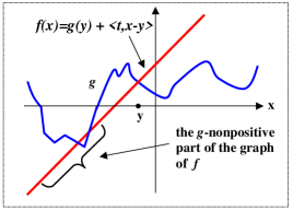
Figure 1: The first geometric interpretation of zero-convexity: using the graph (Remark 1).

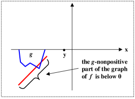
Figure 2: The setting of Figure 2 after the $g$-positive parts of $f$ and $g$ were removed.

Second interpretation: using separating hyperplanes: This interpretation holds only when $y\notin g^{\leq 0}$. We assume also that $g^{\leq 0}\neq\emptyset$. See Figure 3. In this case (2.1) implies that if $g$ is zero-convex at $y$ with a 0-subgradient $t$, then $t\neq 0$ (otherwise $g(y)\leq 0$ because of (2.1), a contradiction) and for each $\omega\in(0,1]$ the hyperplane

$$M(t,\omega):=\{x\in H|\,\,\langle t,x-y\rangle=-\omega g(y)\}$$ (2.2)

strictly separates $y$ from $g^{\leq 0}$. On the other hand, as proved Proposition 1(c) below, if $g^{\leq 0}$ is closed and convex, then $g$ is zero-convex at each point and any (closed) hyperplane separating $y\notin g^{\leq 0}$ from $g^{\leq 0}$ (including $M(t,\omega)$) allows us to find a 0-subgradient $t\in\partial^{0}g(y)$ and to express it explicitly. In fact, any multiplication of this $t$ by a scalar greater than 1 remains a 0-subgradient as follows from Proposition 2(g) below. Thus, at least when $g^{\leq 0}$ is nonempty, closed and convex, there is a certain duality between the 0-subgradients of $g$ at points $y\notin g^{\leq 0}$ and (closed) separating hyperplanes between $g^{\leq 0}$ and these points $y$. The freedom in the choice of the separating hyperplane yields a freedom in the choice of $t$, and this freedom may help in practice.

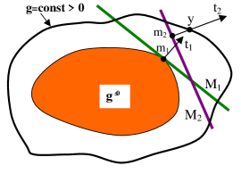
Figure 3: The second geometric interpretation of zero-convexity: using separating hyperplanes (Remark 1). The 0-subgradients can be expressed explicitly using (2.3).

Remark 2

To the best of our knowledge, our generalizations of the subgradient inequality and the subdifferential in Definition 1 are new. Several other generalizations or variations of the standard notion of subdifferential have been considered in the literature, e.g., the Clarke subdifferential (Clarke1983, , pp. 25–27), CSLW1998 , the Fréchet and Hadamard subdifferentials Rockafellar1979 , the $G$-subdifferential Ivanov2004 , the $H$-subdifferential Martinez-Legaz1988 , Mordukhovich’s Subdifferential Mordukhovich1976 ; Soleimani-damaneh2010 , Plastria’s lower subdifferential Plastria , the Quasi-subdifferential GreenbergPierskalla , the Q-subdifferential MartinezLegazSach , the $\Phi$-subdifferential PallaschkeRolewicz1997 , the star-subdifferential Penot1998 , the $\epsilon$-subdifferential MonteiroSvaiter2013 , generalizations of the subgradient inequality such as the notion of invexity Ben-IsraelMond1986 ; Hanson1981 or other notions related to convexity such as approximate convexity DJL2009 ; NgaiLucThera . For a survey on some of these concepts see BorweinZhu1999 .

Remark 3

Computation of $\partial^{0}g$ is not always a simple task but we do have a theoretical method which enables the computation of an element in $\partial^{0}g(y)$ for each $y\in\Omega$ whenever $g^{\leq 0}$ is closed and convex. The method is as follows. If $y\in g^{\leq 0}$, then we simply take $t=0$. If $y\notin g^{\leq 0}$, then we can take

$$t=\frac{g(y)}{\|y-m\|^{2}}(y-m),$$ (2.3)

where $M$ is any (closed) hyperplane which separates $y$ from $g^{\leq 0}$ and $m\in M$ is the orthogonal projection of $y$ onto $M$. See Figure 3 above for an illustration and Proposition 1(c) below for a proof.

The examples given in this section, together with the propositions and their proofs given in Section 3 and the computations given in Section 7, illustrate further some of the techniques of computation. In this connection we note that if one knows how to compute $G(y):=d(y,g^{\leq 0})$, then this yields a convex function whose 0-level-set coincides with $g^{\leq 0}$, and at least for the purpose of the CFP, one may want to use $G$ instead of $g$. However, as already said in Section 1, usually this computation is not simple, and, in addition, it may result in either a complicated function $G$ or complicated (standard) subgradients. Nevertheless, if $G$ can be computed, then one also has an additional way to compute 0-subgradients of $g$ (see Proposition 1(d)) and this freedom may help in practice.

Example 1

Any convex function $g:H\to\mathbb{R}$ having at least one point of continuity is zero-convex at any $y\in H$. This is so because in this case (VanTiel1984, , p. 76) it has a standard subgradient at $y$ and the standard subgradient inequality

$$g(y)+\langle t,x-y\rangle\leq g(x)$$ (2.4)

implies that $g(y)+\langle t,x-y\rangle\leq 0$ whenever $x\in g^{\leq 0}$, that is, (2.1) holds with a standard subgradient $t\in\partial g(y)$. In particular $g$ is zero-convex at any $y\in H$ whenever $H=\mathbb{R}^{n}$ because by (VanTiel1984, , p. 70) the finite dimensionality of $H$ implies that $g$ is continuous everywhere.

In general, whenever $g:\Omega\to\mathbb{R}$ has a standard subgradient $t$ at some $y\in\Omega$, then $t$ is a 0-subgradient of $g$ no matter what subset is $\Omega$. This is true even if $g$ is not convex but (2.4) holds. In this connection, Corollary 1 below implies that any lower semicontinuous quasiconvex function is zero-convex.

Example 2

Any nonpositive function $g$ is zero-convex at every $y\in\Omega$ with $t=0$. However, this class of functions is not interesting for our SSP algorithm (Section 4 below) since in this case any initial point $y$ will satisfy $g_{j}(y)\leq 0$ for all involved functions $g_{j}$, hence the generated sequence will be constant (equal to $y$ itself) which obviously converges to a point in the intersection $C=\cap_{j\in J}\{x\in\Omega\mid g_{j}(x)\leq 0\}$. Additionally, any positive function is zero-convex since (2.1) is void. But again, this is not interesting for our algorithm. However, a nonnegative function having a unique root (like many energy functions) is interesting for our algorithm since it is zero-convex (because its zero-level-set is obviously closed and convex: see Remark 1, second interpretation) and hence, when we apply our algorithm to it, we can find its root, which is also its unique minimum.

Example 3

Let $g:\mathbb{R}\rightarrow\mathbb{R}$ be defined by

$$g(x):=\left\{\begin{array}[c]{ll}\sin x,&\text{for }x\leq\pi/2,\\ 2^{\sin x},&\text{for }x>\pi/2,\end{array}\right.$$ (2.5)

and let $y=\pi/2$. Then $g$ has a discontinuity at $y$. However, $g$ is zero-convex at $y$ with respect to $t=4/\pi$. Indeed, if $g(x)\leq 0$, then $x\leq 0$. Therefore (2.1) holds:

$$g(y)+\langle t,x-y\rangle=1+4x/\pi-2<x\leq 0.$$ (2.6)

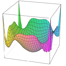
Figure 4: An illustration of the polynomial of Example 4.

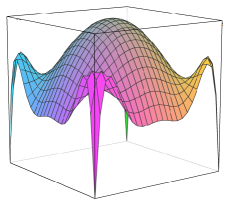
Figure 5: Another illustration of the polynomial, now from the reverse perspective.

Example 4

Let $g:\mathbb{R}^{2}\rightarrow\mathbb{R}$ be defined by

$$g(x_{1},x_{2})=x_{1}^{2}+x_{2}^{2}-x_{1}^{4}x_{2}^{4}+x_{1}^{6}x_{2}^{6}/4-0.3.$$ (2.7)

Elementary calculations (checking the principal minors and using polar coordinates) show that $g$ is convex on the disk $D_{1}=\{(x_{1},x_{2})\mid\,x_{1}^{2}+x_{2}^{2}<0.7^{2}\}$ and that $g^{\leq 0}\subseteq D_{2}=\{(x_{1},x_{2})\mid x_{1}^{2}+x_{2}^{2}\leq 0.6^{2}\}$. In addition, it is evident from Figures 5 and 5 that $g$ is not quasiconvex. As for the computation of the 0-subgradients of $g$, if $y=(y_{1},y_{2})\in D_{1}$, then we can simply take standard subgradients, thus,

$$t=\nabla g(y)=(2y_{1}-4y_{1}^{3}y_{2}^{4}+1.5y_{1}^{5}y_{2}^{6},2y_{2}-4y_{2}^{3}y_{1}^{4}+1.5y_{2}^{5}y_{1}^{6}).$$ (2.8)

For $y\notin D_{1}$, we use (2.3). The line $M$ passing through the projection $m=(0.6y)/\|y\|$ of $y$ on $D_{2}$ and orthogonal to $y-m$ separates $y$ and $g^{\leq 0}$. Thus from (2.3) we conclude that

$$t=\frac{g(y)(y-m)}{\|y-m\|^{2}}=\frac{g(y)}{\|y\|(\|y\|-0.6)}(y_{1},y_{2})$$ (2.9)

is in $\partial^{0}g(y)$. As said in Section 1, inequalities involving nonconvex polynomials (sometimes of high degree) appear in optimization problems HenrLassCSM2004 ; HenrLass-Bookchap-2005 ; HenrLassTAC2012 ; HildebrandKoppe2013 ; LassSIOPT2001 and related fields such as economics and operations research ADSZ2010 ; CambiniMartein2009-book .

Example 5

Let $H$ be a real Hilbert space and $\Omega$ be a nonempty closed and convex subset of $H$. Let $p\in\Omega$ and $A\subseteq H$ be given. Suppose that the distance $d(p,A)$ between $p$ and $A$ is positive. Define a function $g:\Omega\rightarrow\mathbb{R}$ by

$$g(x):=d(x,p)-d(x,A),\quad\forall x\in\Omega.$$ (2.10)

This function (or, actually, the so obtained family of functions) is zero-convex. Indeed, as said in Remark 1 (second interpretation), it suffices to show that $g^{\leq 0}$ is closed and convex (it is nonempty because $p\in g^{\leq 0}$). Now, since $g^{\leq 0}=\{x\in H\mid d(x,p)\leq d(x,A)\}\bigcap\Omega$ and because $\Omega$ is closed and convex, it is sufficient to prove that the first set in the intersection is closed and convex. A computation shows that

$$\{x\in H\mid d(x,p)\leq d(x,A)\}=\bigcap_{a\in A}\{x\in H\mid d(x,p)\leq d(x,a)\}.$$ (2.11)

Since $p\neq a$ for each $a\in A$, each of the members in the above intersection is nothing but the closed half-space whose bounding hyperplane passes through $(p+a)/2$ and orthogonal to $p-a$. Thus $\{x\in H\mid d(x,p)\leq d(x,A)\}$ is the intersection of closed and convex sets, and hence closed and convex.

The zero-level-set of this function $g$ is the, so-called, Voronoi cell of $p$ (restricted to $\Omega$) with respect to the set $A$, and hence $g$ deserves the name “Voronoi function”. A particular and frequently explored case is where the set $A$ consists of finitely many distinct points $p_{1},p_{2},\ldots,p_{\ell}$. These points, together with the given point $p=p_{0}$, are called the sites, and the Voronoi cell corresponding to the site $p_{i}$ is the set $\{x\in\Omega\mid d(x,p_{i})\leq d(x,p_{j}),\quad\forall j\neq i\}$. The collection of these cells is the Voronoi diagram induced by the sites. Voronoi diagrams have numerous applications in science and technology, see, e.g., Aurenhammer ; VoronoiWeb ; OBSC . As can be seen from these surveys, Voronoi diagrams have applications also when the sites are assumed to have more general shapes than points, such as lines segments, balls, and so on, and hence in this case the set $A$ may be infinite. Traditionally, Voronoi diagrams have been investigated in finite-dimensional spaces (especially in $\mathbb{R}^{2}$ and $\mathbb{R}^{3}$), but recently they have been investigated in infinite-dimensional spaces too KopeckaReemReich ; ReemISVD09 ; ReemGeometricStabilityArxiv , and several real-world and theoretical applications were mentioned there.

Returning to $g$, it can be shown, using the triangle inequality, that $\left|g(x)\right|\leq\sup_{a\in A}\|p-a\|$ for every $x\in\Omega$ (in fact, because $\{p\}$ is a singleton, the right-hand side is equal to the Hausdorff distance between $\{p\}$ and $A$). Thus, when $A$ is bounded, then $g$ is bounded on $\Omega$. However, if in addition $\Omega=H$, then this implies that $g$ cannot be convex. Indeed, assume by way of negation that $g$ is convex. Then because it is proper (since it is finite) and lower semicontinuous (actually continuous), it can be represented as the pointwise supremum of a nonempty family of continuous affine functions (VanTiel1984, , p. 91). Since $g$ is non-constant, at least one member $h$ in this family of affine functions must be non-constant. In other words, there exist $0\neq v\in H$ and $\alpha\in\mathbb{R}$ such that $h:=\langle v,\cdot\rangle+\alpha$ satisfies $h(x)\leq g(x)$ for all $x\in\Omega$. But $\lim_{t\to\infty}h(tv)=\infty$. Thus $g$ is not bounded, a contradiction to what was established before.

As a matter of fact, frequently $g$ is not even quasiconvex. Indeed, just consider the simple case where $\Omega=H=\mathbb{R}^{2}$, $p=(0,0)$, $A=\{(0,1)\}$. Then for $x=(-1,1),$ $z=(1,1)$, and $y=(0,1)$ we have $y\in[x,z]$ but $g(x)=g(z)=\sqrt{2}-1<1=g(y)$. The same argument holds whenever $A$ contains an isolated point and the dimension of the space is at least 2 and $\Omega=H$. It can hold even if $A$ does not have any isolated point: just take $p,x,y,z,\Omega,H$ as above but either $A=\{0\}\times[0.5,1]$ or $A=\{0\}\times[0.5,\infty)$. However, in some symmetric configurations $g$ may be quasiconvex: for instance, when $A$ is a sphere, $p$ is the center of the corresponding ball, and $\Omega=H$.

Computation of the 0-subgradients of $g$ is possible by the description mentioned in Remark 3 (especially equality (2.3)). If $y\in g^{\leq 0}$, then obviously $0\in\partial^{0}g(y)$. Otherwise, the definitions of $g$ and $g^{\leq 0}$ imply that there exists an $a\in A$ such that $\|y-a\|<\|y-p\|$. If we denote by $M$ the bisector between $p$ and $a$, namely the set of all points in $H$ having equal distance to $p$ and to $a$, then $M$ is a hyperplane which is the boundary of the half-space $\{x\in H\mid d(x,p)\leq d(x,a)\}$. The point $y$ is located strictly inside the other half-space $\{x\in H\mid d(x,a)\leq d(x,p)\}$. Since $g^{\leq 0}$ is contained in $\{x\in H\mid d(x,p)\leq d(x,a)\}$ (as explained in (2.11) and above it) it follows that $M$ is a hyperplane separating $y$ and $g^{\leq 0}$. Let $m$ be the orthogonal projection of $y$ onto $M$. By (2.3) it follows that $t=g(y)(y-m)/\|y-m\|^{2}$ is in $\partial^{0}g(y)$.

It is possible to represent $t$ in a more convenient way. Indeed, note that the hyperplane $M$ defined above can be represented explicitly as $M=\{x\in H\mid\langle x-u_{0},v\rangle=0\}$ where $u_{0}=0.5(a+p)$ and $v=(a-p)/\|a-p\|$. Since $m$ is the orthogonal projection of $y$ onto $M$ we can write $y=m+\beta v$ where $\beta$ is some real number. This and the Pythagoras theorem imply the identity $\|y-u_{0}\|^{2}=\beta^{2}+\|y-\beta v-u_{0}\|^{2}$, from which it follows that $\beta=\langle y-u_{0},v\rangle$. From (2.3) we conclude that

$$t=\frac{g(y)v}{\beta}=\frac{g(y)(a-p)}{\langle y-0.5(a+p),a-p\rangle}.$$ (2.12)

This $t$ depends on $y$ but also on $a$. By an appropriate selection of $a\in A$ we can ensure that $\|t\|\leq 4$. In fact, we can even ensure that $\|t\|$ will be bounded above by a number arbitrarily close to 2 and sometimes even by 2 (when $d(y,A)$ is attained). Indeed, assume $y\notin g^{\leq 0}$. Let $\epsilon\in(0,0.5g(y))$ be arbitrary. Let $a\in A$ be chosen such that

$$d(y,a)<d(y,A)+\epsilon.$$ (2.13)

From the definition of $g$ and the triangle inequality we see that any point $x$ in the open ball of radius $0.5g(y)-\epsilon$ around $y$ satisfies

$$d(x,a)\leq d(x,y)+d(y,a)<0.5g(y)-\epsilon+d(y,A)+\epsilon\\ \leq d(y,p)-g(y)+0.5g(y)\leq d(y,x)+d(x,p)-0.5g(y)<d(x,p),$$ (2.14)

and hence $x$ belongs to the half-space to which $y$ belongs. Recalling that $|\beta|=\|y-m\|$ and that $m$ is in the other half-space, we have $|\beta|\geq 0.5g(y)-\epsilon$. This and (2.12) show that

$$\|t\|\leq\frac{g(y)}{0.5g(y)-\epsilon}.$$ (2.15)

This proves the claim since $\epsilon$ can be arbitrary small and we can select the appropriate $a\in A$ as above so that (2.13) and hence (2.15) will be satisfied. In particular, by taking $\epsilon=0.25g(y)$ we obtain $\|t\|\leq 4$. If in addition $d(y,A)=d(y,a)$ for some $a\in A$, then by choosing this $a$ and mimicking the previous analysis with $\epsilon=0$ we see that $\|t\|\leq 2$.

Example 6

The functions described below are variations of the Voronoi function defined in (2.10). They deserve some attention since a particular case of them will be used in Section 7.

One variation is obtained by replacing $p$ by a subset $P$ and taking

$$g(x):=g_{P,A}(x)=d(x,P)-d(x,A).$$ (2.16)

See Aurenhammer ; VoronoiWeb ; KopeckaReemReich ; OBSC ; ReemGeometricStabilityArxiv and the references therein for some applications of Voronoi cells defined in this way. In general, the Voronoi cell $g^{\leq 0}$ is closed ($g$ is 2-Lipschitz) but not convex. However, in some cases it is convex, e.g., when $\Omega=H=\mathbb{R}^{2}$, $A=\{(-1,0),(0,-1),(1,-1),(0,1),(1,1),(2,0)\}$, and $P=\{(0,0),(1,0)\}$.

Another variation is to consider weighted distances, namely, we assign to each $a\in A$ a real number $w_{a}$ (a weight), and assign a weight $w_{p}$ to $p$. For every $x\in\Omega$ and $a\in A$ let

$$\begin{array}[c]{lll}d_{p}(x)&:=&\|x-p\|-w_{p},\\ d_{a}(x)&:=&\|x-a\|-w_{a},\\ d_{A}(x)&:=&\inf\{d_{a}(x)\mid a\in A\},\end{array}$$ (2.17)

and define the additively weighted Voronoi function

$$g(x):=g_{w}(x):=d_{p}(x)-d_{A}(x).$$ (2.18)

The 0-level-set $g^{\leq 0}$ is the additively weighted Voronoi cell of the site $p$. It is closed since $d_{A}$ is upper semicontinuous and hence $g$ is lower semicontinuous. In molecular biology GPF1997 ; KWCKLBK2006 ; RKCPK2005 the site $p$ represents the center of a spherical atom (or molecule) whose van der Waals radius is $w_{p}$. Hence $d_{p}(x)$ is the distance from $x$ to the sphere for each $x$ outside the corresponding ball. Similarly, each $a\in A$ represents the center of a spherical atom (or molecule) whose van der Waals radius is $w_{a}$. In crystallography and stochastic geometry the common name to additively weighted Voronoi diagrams is Johnson-Mehl tessellation (or model). In this model $p$ (and each $a\in A$) represent a nucleation center from which a crystal starts to grow in a uniform way in all directions, but the growing process starts at different times from each nucleation center. In this case $w_{p}$ is minus the starting time of the growth from $p$ and $w_{a}$ is minus the starting time of the growth from $a$. See, e.g., CSKM2013 ; OBSC and the references therein. See also Section 7 below for a concrete computational result in the molecular biology context.

Under certain assumptions on the parameters the function $g$ defined in (2.18) is zero-convex. For instance, assume that $A=\{a\}$, $a\in H$ is given, and that

$$w_{p}\leq w_{a}<\|a-p\|+w_{p}.$$ (2.19)

Let $B$ be the ball of radius $w_{a}-w_{p}$ around $a$ (degenerates to a point when $w_{a}=w_{p}$). We claim that under these assumptions

$$g^{\leq 0}=G^{\leq 0}$$ (2.20)

where $G(x)=d(x,p)-d(x,B)$ for all $x\in\Omega$. Indeed, if $x\notin B$, then we have the equality $G(x)=d(x,p)-(d(x,a)-(w_{a}-w_{p}))=g(x)$. Hence the intersection of both sides of (2.20) with the complement of $B$ coincide. If $x\in B$, then $G(x)=d(x,p)$ and hence $x\in G^{\leq 0}$ would imply that $x=p$, a contradiction to $p\notin B$ (by (2.19)). Therefore $x\notin G^{\leq 0}$. However, the assumption $x\in B$ implies $d(x,a)\leq w_{a}-w_{p}$. Hence $x$ cannot belong to $g^{\leq 0}$ because this would imply that $d(x,p)\leq d(x,a)-(w_{a}-w_{p})\leq 0$, and again $x=p$, a contradiction. We conclude that (2.20) holds. Since we already know from Example 5 that $G^{\leq 0}$ is convex, it follows that $g^{\leq 0}$ is convex. Since $g^{\leq 0}$ is closed, Remark 1 (second interpretation) implies that $g$ is zero-convex. Geometrically (at least when $\Omega$ is, say, the whole space or it is a cube containing $p$ and $a$ in its interior), the boundary of $g^{\leq 0}$ is the intersection of $\Omega$ with the (possibly infinite dimensional) hyperboloid $\{x\in H\,|\,d(x,p)-d(x,a)=w_{p}-w_{a}\}$. In addition, $p\in g^{\leq 0}$. When $w_{p}=w_{a}$, the hyperboloid degenerates to a hyperplane.

We finish this example by noting that there are other weighted versions of Voronoi diagrams. One of them is the multiplicative weighted distance in which $d_{p}(x)=d(x,p)/w_{p}$ and $d_{a}(x)=d(x,a)/w_{a}$ for some given positive weights $w_{p}$ and $w_{a}$. This version is used in molecular biology, e.g., in GTL1995 , where again $w_{p}$ and $w_{a}$ are the van der Waals radii of the involved atoms/molecules. See also Aurenhammer ; OBSC .

3 Zero-convex functions: Properties

In this section we present several properties of zero-convex functions and discuss theoretical ways of constructing their 0-subgradients.

Proposition 1

Let $H$ be a real Hilbert space and let $\Omega$ be a nonempty convex subset of $H$. Let $g:\Omega\rightarrow\mathbb{R}$ be given.

1. The function $g$ is zero-convex at $y\in\Omega$ with respect to some $t\in\partial^{0}g(y)$ if and only if there exists a function $\psi:\mathbb{R}\rightarrow\mathbb{R}$ satisfying $\psi(r)\leq 0$ for all $r\leq 0$ such that

   $$g(y)+\langle t,x-y\rangle\leq\psi(g(x)),\quad\forall x\in g^{\leq 0}.$$ (3.1)

2. If $g$ is zero-convex, then its zero-level-set $g^{\leq 0}$ is convex.

3. If $g^{\leq 0}$ is closed and convex, then $g$ is zero-convex. In fact, if $y\in g^{\leq 0}$, then $0\in\partial^{0}g(y)$, and if $y\notin g^{\leq 0}$, then for

   $$t=\frac{g(y)}{\|y-m\|^{2}}(y-m),$$ (3.2)

   we have $t\in\partial^{0}g(y)$ where $m\in M$ is the orthogonal projection of $y$ onto a (closed) hyperplane $M$ strictly separating $y$ from $g^{\leq 0}$.

4. If $m$ is the (unique) orthogonal projection of $y\notin g^{\leq 0}$ onto $g^{\leq 0}$, then for $t$ defined in (3.2) we have $t\in\partial^{0}g(y)$.

Proof

It can be assumed that $g^{\leq 0}\neq\emptyset$, otherwise the assertion holds trivially (void).

1. If there exists such a function $\psi$, then (3.1) implies (2.1) since $g(x)\leq 0$ implies $\psi(g(x))\leq 0$. Hence $g$ is zero-convex at $y$ and $t\in\partial^{0}g(y)$. Conversely, if $g$ is zero-convex at $y$ and $t\in\partial^{0}g(y)$, then (3.1) is satisfied with any function $\psi:\mathbb{R}\rightarrow\mathbb{R}$ satisfying $\psi(r)=0$ whenever $r\leq 0$.

2. Suppose, by way of negation, that $g^{\leq 0}$ is not convex. Then there exist two distinct points $x_{1},$ $x_{2}\in g^{\leq 0}$ such that for some $y$ in the line segment $[x_{1},x_{2}]$ we have $y\notin g^{\leq 0}$, namely $g(y)>0$. Since $g$ is zero-convex on the convex subset $\Omega,$ thus at $y,$ there is a point $t\in H$ such that (2.1) holds. This and the fact that $g(x_{i})\leq 0$, $i=1,2,$ imply that the function

   $$f(x):=g(y)+\langle t,x-y\rangle$$ (3.3)

   satisfies $f(x_{i})\leq 0$, $i=1,2$. Since $f(x)$ is convex and $y\in[x_{1},x_{2}]$ we also have $f(y)\leq 0$. This is a contradiction since $f(y)=g(y)>0$.

3. Given $y\in\Omega$, distinguish between the cases $y\in g^{\leq 0}$ or $y\notin g^{\leq 0}$. In the first case define $t:=0$. Then for any $x\in g^{\leq 0}$ we obviously have

   $$g(y)+\langle t,x-y\rangle\leq 0+0,$$ (3.4)

   hence, (2.1) is satisfied. Now consider the case $y\notin g^{\leq 0}$. Since $g^{\leq 0}$ is closed and convex, the Hahn-Banach theorem, in one of its geometric versions (VanTiel1984, , p. 38), ensures that there exists a hyperplane $M$ strictly separating $y$ from $g^{\leq 0}$. The hyperplane $M$ is guaranteed to be a closed set and, actually, it can be written as $M=\{x\in H\mid\langle e,x-m\rangle=0\}$ where $m\in M$ is the orthogonal projection of $y$ onto $M$ and $e=(y-m)/\|y-m\|$. We have the decomposition $H=M\cup H_{1}\cup H_{2}$ where $H_{1}=\{x\in H\mid\langle e,x-m\rangle>0\}$ and $H_{2}=\{x\in H\mid\langle e,x-m\rangle<0\}$. By the definition of $m$, $M$, and $e$ it follows that $y\in H_{1}$ and $g^{\leq 0}\subseteq M\cup H_{2}$. Let $\beta:=g(y)/\|y-m\|$ and $t:=\beta e$, as in (3.2). Since $g(y)>0$ we have $\beta>0$. The above implies that for each $x\in g^{\leq 0}$

   $$g(y)+\langle t,x-y\rangle=\langle t,y-m\rangle+\langle t,x-y\rangle=\beta\langle e,x-m\rangle\leq 0,$$ (3.5)

   thus, (2.1) is satisfied again. As a matter of fact, by translating $M$ slightly towards $y$ we can even ensure that $g^{\leq 0}\subset H_{2}$ and so (3.5) will be satisfied with strict inequality.

4. Because $m$ is the orthogonal projection of $y\notin g^{\leq 0}$ onto $g^{\leq 0}$ (whose existence and uniqueness are well-known, see, e.g., GG-book-1981 ), then the hyperplane $M$ which passes through $m$ and is orthogonal to $y-m$ strictly separates $y$ and $g^{\leq 0}$. Indeed, since $\langle y-m,y-m\rangle>0$ (otherwise $y\in g^{\leq 0}$) we have $y\in H_{1}=\{x\in H\mid\langle y-m,x-m\rangle>0\}$. We can write $M=\{x\in H\mid\langle y-m,x-m\rangle=0\}$ and we have the decomposition $H=M\cup H_{1}\cup H_{2}$ where $H_{2}=\{x\in H\mid\langle y-m,x-m\rangle<0\}$. A well-known characterization of the orthogonal projection $m$ of a point $y$ onto a nonempty, closed and convex subset says that $\langle y-m,x-m\rangle\leq 0$ for every $x$ in the subset (see (BauschkeCombettes2011, , p. 46)). Therefore $g^{\leq 0}\subseteq M\cup H_{2}$ and hence $g^{\leq 0}\cap H_{1}=\emptyset$. Thus $M$ strictly separates $y$ and $g^{\leq 0}$ and the assertion follows from part (c).

Remark 4

An alternative but somewhat related approach to the fact that the convexity of $g^{\leq 0}$ implies the zero-convexity of $g$, based on an idea of Benar Svaiter SvaiterPC2011 , is as follows. Assume that $g^{\leq 0}\neq\emptyset$, otherwise the assertion holds trivially (void). Define the distance from $x$ to $g^{\leq 0}$ as $f(x):=d(x,g^{\leq 0})$ for each $x$. This continuous function is also convex since $g^{\leq 0}$ is convex. Hence, as is well-known (VanTiel1984, , p.76), it has a (standard) subgradient $s$ at any $y$. Let $t:=cs$ where

$$c:=\left\{\begin{array}[c]{ll}g(y)/f(y),&\text{if }f(y)\neq 0,\\ 0,&\text{otherwise.}\end{array}\right.$$ (3.6)

Note that $f(y)=0$ if and only if $y\in g^{\leq 0}$ because $g^{\leq 0}$ is closed. This implies (2.1) when $y\in g^{\leq 0}$ with $t=0$ (as in (3.4)). When $y\notin g^{\leq 0}$ we have $f(y)>0$, $g(y)>0$, and $t=(g(y)/f(y))s$. By the subgradient inequality, which $f$ satisfies, we have

$$f(y)+\langle s,x-y\rangle\leq f(x)=0,\quad\forall x\in g^{\leq 0}.$$ (3.7)

This implies (2.1) after multiplying this inequality by $c=g(y)/f(y)$.

Corollary 1

Let $H$ be a Hilbert space and $\Omega\subseteq H$ be nonempty, closed, and convex. Any lower semicontinuous function $g:\Omega\to\mathbb{R}$ having a convex zero-level-set is zero-convex. In particular, if $g$ is lower semicontinuous and quasiconvex, then it is zero-convex.

Proof

It can be assumed that $g^{\leq 0}\neq\emptyset$, otherwise the assertion holds trivially (void). Since $g$ is lower semicontinuous $g^{\leq 0}$ is closed in $\Omega$ (in the topology induced by the norm) and hence ($\Omega$ is closed) in $H$. Thus, when $g^{\leq 0}$ is assumed to be convex the assertion follows from Proposition 1(c). The assertion about lower semicontinuous quasiconvex functions is a consequence of Proposition 1(c) and the fact that all their level-sets are closed and convex.

Proposition 2

Let $H$ be a real Hilbert space and let $\Omega$ be a nonempty convex subset of $H$.

1. If $g:\Omega\rightarrow\mathbb{R}$ is zero-convex at $y$ with respect to both $t_{1}\in\partial^{0}g(y)$ and $t_{2}\in\partial^{0}g(y)$, then it is zero-convex at $y$ with respect to any convex combination of $t_{1}$ and $t_{2}$.

2. Suppose that $g:\Omega\rightarrow\mathbb{R}$ is zero-convex at $y$ with respect to some $t\in\partial^{0}g(y)$. Given $\alpha\geq 0$, the function $\tilde{g}:=\alpha g$ is zero-convex at $y$ with respect to $\tilde{t}=\alpha t$.

3. Suppose that $g_{1},g_{2},\ldots,g_{m}$ are given zero-convex functions at $y$. Then the envelope of $\{g_{i}\}_{i=1}^{m}$, defined by $g(x):=\max\{g_{i}(x)\mid\,i=1,2,\ldots,m\}$, is also zero-convex at $y$.

4. Suppose that $\{g_{i}|\,\,i\in I\}$ is a family of (possibly infinitely many) lower semicontinuous zero-convex functions defined on a closed subset $\Omega$ of $H$. Then $g=\sup\{g_{i}\mid i\in I\}$ is zero-convex.

5. Suppose that $g:\Omega\rightarrow\mathbb{R}$ is zero-convex and that it has a closed zero-level-set. Let $\psi:\mathbb{R}\rightarrow\mathbb{R}$ be a function satisfying $\psi(r)\leq 0$ if and only if $r\leq 0$. Then the composite function $\psi\circ g$ is zero-convex. In particular the above holds when $\Omega$ is closed, $g$ is lower semicontinuous and zero-convex, and $\psi$ satisfies the above-mentioned property.

6. Suppose that $g:\Omega\rightarrow\mathbb{R}$ has a nonempty zero-level-set. If $g$ is zero-convex at $y$ and if $g(y)>0$, then any 0-subgradient $t\in\partial^{0}g(y)$ satisfies $t\neq 0$.

7. Suppose that $f:\Omega\rightarrow\mathbb{R}$ and $g:\Omega\rightarrow\mathbb{R}$ are zero-convex at $y\in\Omega$ and that their zero-level-sets coincide. If $y$ is outside the zero-level-set and $t\in\partial^{0}f(y)$, then $ct\in\partial^{0}g(y)$ for any $c\geq g(y)/f(y)$. In particular, if $t\in\partial^{0}g(y)$, then so does $ct$ for all $c\geq 1$.

Proof

1. Follows from multiplication of (2.1) by each of the convex combination coefficients and adding the resulting inequalities.

2. Follows from multiplication of (2.1) by $\alpha$.

3. For each $i$ consider the associated subgradient $t_{i}\in\partial^{0}g_{i}(y)$. Let $j$ be the index for which $g(y)=g_{j}(y)$ and let $t=t_{j}$. Suppose that $x\in H$ satisfies $g(x)\leq 0$. Then $g_{j}(x)\leq 0$, thus, by (2.1),

   $$\langle t,x-y\rangle+g(y)=\langle t_{j},x-y\rangle+g_{j}(y)\leq 0,$$ (3.8)

   as required.

4. Let $x_{1},x_{2}\in g^{\leq 0}$. Then $g_{i}(x_{1})\leq g(x_{1})\leq 0$ and $g_{i}(x_{2})\leq 0$ for any $i\in I$. From the convexity of the zero-level-set of $g_{i}$ (Proposition 1(b)) it follows that $g_{i}(x)\leq 0$ for all $x$ in the line segment $[x_{1},x_{2}]$ and all $i$. Thus $g(x)\leq 0$ and hence $g^{\leq 0}$ is convex. It is well-known and not hard to verify that $g$ is lower semicontinuous. Therefore, Corollary 1 implies that $g$ is zero-convex.

5. By assumption $g^{\leq 0}$ is closed and by Proposition 1(b) it is convex. By the nature of $\psi$ the zero-level-sets of $g$ and of $\psi\circ g$ coincide. Thus Proposition 1(c) implies that $\psi\circ g$ is zero-convex. Finally, if $\Omega$ is closed and $g$ is also lower semicontinuous, then $g^{\leq 0}$ is closed and the assertion follows from the above discussion.

6. Let $t\in\partial^{0}g_{i}(y)$ and assume, to the contrary, that $t=0$. If $x\in\Omega$ satisfies $g(x)\leq 0$, then by (2.1)

   $$0<g(y)=g(y)+\langle t,x-y\rangle\leq 0,$$ (3.9)

   which is a contradiction.

7. From (2.1) and the equality between the zero-level-sets of the functions we have the inequality $\langle t,x-y\rangle\leq-f(y)$ for any $x\in g^{\leq 0}$. In addition, $f(y)>0$, thus,

   $$g(y)+\langle ct,x-y\rangle\leq g(y)-cf(y)\leq 0,$$ (3.10)

   by the choice of $c$. Therefore, $ct\in\partial^{0}g(y)$. Finally, by taking $f=g$ in the previous case, we conclude that if $t\in\partial^{0}g(y)$, then $ct\in\partial^{0}g(y)$ for any $c\geq 1$.

For later use (see, e.g., the discussion after Condition 3 below) we present a few propositions which give sufficient conditions for the existence of bounded 0-subgradients. These propositions also give some ideas regarding the way of computing 0-subgradients in certain settings. The first proposition is a generalized variation of an assertion hidden in the proof of (bb96, , Proposition 7.8, (ii)$\Longrightarrow$(iii)) (namely, that the subgradients of a convex and Lipschitz function are uniformly bounded by the Lipschitz constant).

Proposition 3

Let $H$ be a real Hilbert space and let $\Omega$ be nonempty, closed and convex. Suppose that $g:\Omega\rightarrow\mathbb{R}$ is zero-convex and Lipschitz on $\Omega$ with a Lipschitz constant $\alpha>0$ and that $g^{\leq 0}\neq\emptyset$. Then for each $y\in\Omega$ there exists $t\in\partial^{0}g(y)$ satisfying $\|t\|\leq\alpha$. As a matter of fact, for each $y\notin g^{\leq 0}$ there exists $t\in\partial^{0}g(y)$, defined by (3.2), satisfying

$$\|t\|\leq\alpha\frac{\|y-z\|}{\|y-m\|},$$ (3.11)

where $m\in M$ is the projection of $y$ onto a closed hyperplane strictly separating $y$ from $g^{\leq 0}$, and $z\in g^{\leq 0}$ is arbitrary. In particular, the above holds if $\Omega$ is contained in an open subset of $H$ and $g$ is Gâteaux-differentiable on this open set and its derivative is uniformly bounded by some $\alpha>0$.

Proof

If $y\in g^{\leq 0}$, then we can take $t=0$. Otherwise, let $t\in\partial^{0}g(y)$ be defined as in (3.2) where $m\in M$ is the projection of $y$ onto a closed hyperplane $M$ strictly separating $y$ from $g^{\leq 0}$, the existence of which is ensured by the Hahn-Banach theorem since $g^{\leq 0}$ is closed ($g$ is continuous and $\Omega$ is closed) and convex (Proposition 1(b)). From (3.2) we have $\|t\|=g(y)/\|y-m\|$. Let $z\in g^{\leq 0}$ be given. Since $g(z)\leq 0$ and $g(y)>0$, the fact that the Lipschitz constant of $g$ is $\alpha$ implies that

$$\|t\|\leq\frac{(g(y)-g(z))\|y-z\|}{\|y-z\|\|y-m\|}\leq\alpha\frac{\|y-z\|}{\|y-m\|}.$$ (3.12)

In particular, the above is true when $m$ is the best approximation (orthogonal) projection of $y$ onto $g^{\leq 0}$ and $M$ passes through $m$ and is orthogonal to $y-m$ (see the proof of Proposition 1(d)). By taking $z=m$ we have $\|t\|\leq\alpha$, as claimed. Finally, a well-known consequence of the mean value theorem says that when $g$ is Gâteaux-differentiable and its derivative is bounded by some constant, then $g$ is Lipschitz with this constant (AmbroProdi-Book-1993, , Theorem 1.8, p. 13) and hence the assertion follows.

Proposition 4

Let $H$ be a real Hilbert space and let $\Omega$ be nonempty and convex. Let $g:\Omega\rightarrow\mathbb{R}$ be zero-convex. Suppose that $\emptyset\neq g^{\leq 0}\subseteq B(c,r)$ where $B(c,r)$ is the open ball with center $c$ and radius $r>0$. Let $\epsilon>0$ be given. Suppose that $B(c,r+\epsilon)\subset\Omega$ and that $g$ is convex on this ball.

1. If $g$ is Lipschitz on $\Omega$ with constant $\alpha$, then for each $y\in\Omega$ there exists $t\in\partial^{0}g(y)$ satisfying $\|t\|\leq\alpha(1+(2r/\epsilon))$. In fact, if $y\in B(c,r+\epsilon)$, then $t$ can be taken as a standard subgradient and if $y\notin B(c,r+\epsilon)$, then $t$ can be defined by (3.2).

2. If $g$ is bounded on $\Omega$ by some $\beta>0$, then for each $y\in\Omega$ there exists $t\in\partial^{0}g(y)$ satisfying $\|t\|\leq 4\beta/\epsilon$. In fact, if $y\in B(c,r+0.5\epsilon)$, then $t$ can be taken as a standard subgradient, and if $y\notin B(c,r+0.5\epsilon)$, then this $t$ can be defined by (3.2).

Proof

1. Since $g$ is Lipschitz and convex on the ball $B(c,r+\epsilon)$ with a Lipschitz constant $\alpha$, it is known that its standard subgradients at points in this ball are bounded by $\alpha$ (see the proof of (bb96, , Proposition 7.8, (ii)$\Longrightarrow$ (iii)) and replace there $rB_{X}$ by our ball). Any standard subgradient is a 0-subgradient as explained in Example 1 above. Now let $y\in\Omega$, $y\notin B(c,r+\epsilon)$ and consider its projection $m$ onto the closed ball $\overline{B(c,r)}$. Consider also the closed hyperplane $M$ passing through $m$ and orthogonal to $y-m$. This $M$ separates the ball and hence $g^{\leq 0}$ from $y$ and for $t$ defined by (3.2) we know from Proposition 1(c) that $t\in\partial^{0}g(y)$. Let $z\in g^{\leq 0}$ be given. From (3.11), the fact that $z,m\in\overline{B(c,r)}$, and the fact that $\|y-m\|\geq\epsilon$, we have

   $$\|t\|\leq\alpha\frac{\|y-z\|}{\|y-m\|}\leq\alpha\frac{(\|y-m\|+\|m-z\|)}{\|y-m\|}\leq\alpha\left(1+\frac{2r}{\epsilon}\right).$$ (3.13)

   Since the right-hand side of (3.13) is greater than $\alpha$ we conclude that in both cases discussed above we can find $t\in\partial^{0}g(y)$ satisfying $\|t\|\leq\alpha(1+(2r/\epsilon))$.

2. The restriction of $g$ to the ball $B(c,r+\epsilon)$ is a convex function which is bounded by $\beta$, thus it is a known fact (which follows, e.g., from the proof of (VanTiel1984, , Theorem 5.21, p. 69)) that $g$ is Lipschitz on the ball $B(c,r+0.5\epsilon)$ with constant $2\beta/(r+0.5\epsilon-r)=4\beta/\epsilon$. Hence, as explained before, any standard subgradient (which is a 0-subgradient) of a point $y$ in the ball is bounded by this Lipschitz constant. Now consider a point $y$ outside this ball. For $t$ defined by (3.2) we know from Proposition 1(c) that $t\in\partial^{0}g(y)$ and $\|t\|=g(y)/\|y-m\|\leq 2\beta/\epsilon$. The assertion follows.

Remark 5

In general, if some of the above conditions are not satisfied, then uniform boundedness of a selection of 0-subgradients cannot be ensured even if the given function is continuous and quasiconvex. A simple example is $g:\mathbb{R}\to\mathbb{R}$ defined by $g(y)=0$ when $y\leq 0$, and $g(y)=\sqrt{y}$ otherwise. This is a continuous and quasiconvex function, but when $y>0$ and $t\in\partial^{0}g(y)$, it follows from (2.1) (by putting $x=0\in g^{\leq 0}$) that $t\geq 1/\sqrt{y}$.

4 Formulation of the zero-convex feasibility problem and the associated algorithm

In this section we formulate our algorithm for solving the CFP with zero-convex functions. See Section 7 below for a concrete example (including computational results). See also Subsection 1.5 and Section 2 above for related examples.

Let $\Omega$ be a nonempty closed and convex subset of the real Hilbert space $H$. Denote by $P_{\Omega}$ the best approximation (orthogonal) projection onto $\Omega$. Let $J$ be a finite or a countable set of indices. For each $j\in J$, let $g_{j}:\Omega\rightarrow\mathbb{R}$ be a continuous zero-convex function. For each $j\in J$ let

$$C_{j}=\{x\in\Omega\mid g_{j}(x)\leq 0\}$$ (4.1)

and suppose that

$$C=\bigcap_{j\in J}C_{j}\neq\emptyset.$$ (4.2)

Let $\{i(n)\}_{n=0}^{\infty}$ be an infinite sequence indices $i(n)\in J$, henceforth called a control sequence, which is almost cyclic in a generalized sense, i.e., $i:\mathbb{N}\cup\{0\}\rightarrow J$ and for each $j\in J$ there exists an $L_{j}\in\mathbb{N}$ such that the control selects the subset $C_{j}$ at least once in each block of length $L_{j}$ of successive indices of $J$. Formally,

$$\forall j\in J\text{, }\exists L_{j}\in\mathbb{N}\,\text{\ such that }\forall\,\,s\in\mathbb{N}\,\ \text{we have }j\in\{i(s),i(s+1),\ldots,i(s+L_{j}-1)\}.$$ (4.3)

This definition seems to have been introduced by Browder (Browder1967, , Definition 5). See (Combettes1996, , pp. 209–210) for an example with $L_{j}=2^{j},j\in J=\mathbb{N}$. A well-known particular case of (4.3) is the almost cyclic control, namely $J=\{1,2,\ldots,\ell\}$, $\ell\in\mathbb{N}$ is given, and there exists $L\in\mathbb{N}$ such that $L_{j}=L$ for all $j\in J$. The particular case of the almost cyclic control when $L=\ell$ is the cyclic control. For other types of controls which are related to (4.3), see CensorChenPajoohesh2011 .

We consider the following algorithm.

Algorithm 1

 The Sequential Subgradient Projection (SSP) Method with Perturbations

Initialization: $x_{0}\in\Omega$ is arbitrary.

Iterative Step:

$$x_{n+1}=\left\{\begin{array}[c]{ll}P_{\Omega}\left(x_{n}-\displaystyle\lambda_{n}{\frac{g_{i(n)}(x_{n})}{\parallel t_{n}\parallel^{2}}}t_{n}+b_{n}\right),&\text{if }g_{i(n)}(x_{n})>0,\\ x_{n},&\text{if }g_{i(n)}(x_{n})\leq 0,\end{array}\right.$$ (4.4)

where $t_{n}\in\partial^{0}g_{i(n)}(x_{n})$ and $\{b_{n}\}_{n=0}^{\infty}$ is a sequence of elements in $H$.

Relaxation Parameters: $\{\lambda_{n}\}_{n=0}^{\infty}$ is a sequence of real numbers satisfying the inequality

$$\epsilon_{1}\leq\lambda_{n}\leq 2-\epsilon_{2},\quad\forall n\in\mathbb{N}\cup\{0\}$$ (4.5)

for fixed, arbitrarily small, $\epsilon_{1},\epsilon_{2}>0$ satisfying $\epsilon_{1}+\epsilon_{2}\leq 2$.

Control Sequence: $\{i(n)\}_{n=0}^{\infty}$ is almost cyclic in a generalized sense, i.e., it obeys (4.3).

Proposition 2(f) ensures that $t_{n}\neq 0$ whenever $g_{i(n)}(x_{n})>0$, and hence $x_{n+1}$ is well-defined. The elements of the sequence $\{b_{n}\}_{n=0}^{\infty}$ act as perturbation terms in the algorithm. If $b_{n}=0$ for all $n$ then the algorithm is the ordinary feasibility-seeking Cyclic Subgradient Projection (CSP) algorithm of cl82 , at least when the control is almost cyclic and the functions $g_{j}$ are convex. When the first line of (4.4) occurs, then we say that the algorithm makes an active step at step $n+1$. When the second line of (4.4) occurs, then we say that the algorithm makes an inactive step at step $n+1$.

5 Conditions for convergence

For the convergence analysis we will need the following conditions.

Condition 1

For some $\mu>0$ which is any number greater than the distance $d(x_{0},C)$ between $x_{0}$ and $C$, the following inequality is satisfied

$$\parallel b_{n}\parallel\leq\min\left(\mu,\frac{\epsilon_{1}\epsilon_{2}h_{n}^{2}}{2(5\mu+4h_{n})}\right),\quad\forall n\in\mathbb{N},$$ (5.1)

where

$$h_{n}=\left\{\begin{array}[c]{ll}g_{i(n)}(x_{n})/\|t_{n}\|,&\text{if }g_{i(n)}(x_{n})>0,\\ 0,&\text{if }g_{i(n)}(x_{n})\leq 0.\end{array}\right.$$ (5.2)

The construction of the sequence $\{b_{n}\}_{n=0}^{\infty}$ of perturbations is done in an adaptive way, in contrast to other works dealing with inexact algorithms (such as Eckstein1998 ; Rockafellar1976 ) in which such terms satisfy a certain fixed (nonadaptive) condition, e.g., the summability condition $\sum_{n=1}^{\infty}\|b_{n}\|<\infty$ or some other fixed conditions CorvellecFlam ; DES1982 ; SolodovSvaiter2000 ; SolodovSvaiter2001 . In our case one computes $g_{i(n)}(x_{n})$ and $h_{n}$, and then chooses any $b_{n}$ such that (5.1) holds. The only somewhat adaptive perturbation terms that we are aware of appear in the very recent work (OteroIusem2012, , relations (31)–(32)).

It is interesting to note that Condition 1 actually implies that $\sum_{n=1}^{\infty}\|b_{n}\|<\infty$: see Remark 6 below. This means that Condition 1 is less general than summability, but this is not necessarily a bad thing. Indeed, as argued briefly in (SolodovSvaiter2000, , p. 216) and in a more detailed form in SvaiterPC2012 , the summability condition is not satisfactory since it gives too much freedom for the perturbations and hence it may lead to undesired practical results. On the one hand it allows perturbations of the form $b_{n}=n^{100n}$ for each $n\leq 10^{22222}$ and $b_{n}={10000}^{-n}$ for each $n>10^{22222}$, which means essentially no convergence at all in practice. On the other hand, if $b_{n}={10000}^{-n}$ right at the beginning, then this implies that very soon the perturbations will be too small for the computing device to make any difference as perturbations proceed (but usually this will not accelerate the convergence). In contrast, conditions such as Condition 1 guide the user regarding the possible values of the perturbation at the $n$-th iteration. These values are given in terms of previous iterations and they do not depend on future iterations as in the case of the summability condition. In a sense they are more adaptive to the whole problem: they are not too large and not too small.

As a final remark concerning Condition 1, we note that in order to verify (5.1) one has to know $\mu$, i.e., to have an upper bound on the (yet unknown) distance $d(x_{0},C)$. However, in practice, when applying Algorithm 1, one usually restricts the problem to a large closed, bounded, and convex region $\Omega$ (say, a cube or a ball), due to limitations in the computing device, and the diameter of this region can be taken as $\mu$. In other cases one may have better estimates on the value of $\mu$. For instance, if one of the involved subsets $C_{j}$ is bounded, then $C\subseteq C_{j}$ is bounded and one can start from a point $x_{0}$ in $C_{j}$ and take the diameter of $C_{j}$ as $\mu$.

The second condition for convergence is the following.

Condition 2

For each $j\in J$, the function $g_{j}$ is zero-convex, uniformly continuous on closed and bounded subsets of $\Omega$, and weakly sequential lower semicontinuous.

The condition of uniform continuity holds in many cases, e.g., when the space is finite-dimensional (recall that $g_{j}$ is continuous with respect to the norm topology) or when $g_{j}$ satisfies a Lipschitz or Hölder condition. The weakly sequential lower semicontinuity condition holds, for instance, when the space is finite-dimensional, or when $g_{j}$ is quasiconvex (by (BauschkeCombettes2011, , Proposition 10.23) and the assumption that $g_{j}$ is continuous).

The last condition that we need is the following.

Condition 3

There exists a number $K>0$ such that $\|t_{n}\|\leq K$ for all $n\in\mathbb{N}\cup\{0\}$.

It seems that verification of Condition 3 requires knowledge about the functions that define the subsets of the feasibility problem as level-sets. A possible relevant property which may help here is that of uniform boundedness of the subgradients on bounded sets. This property is a standard one, frequently used in theorems on subgradient projection methods, when the functions are convex. If the space is finite-dimensional, then it holds, e.g., if the effective domain of all functions is the whole space and there are finitely many functions, see, e.g., (bb96, , Proposition 7.8 and Corollary 7.9). If the space is infinite-dimensional but the functions are uniformly continuous on closed and bounded subsets (as implied by Condition 2) and all the finitely many functions are convex, then Condition 3 holds too, again from (bb96, , Proposition 7.8). When infinitely many functions are involved in the algorithm and all of them are Lipschitz with uniformly bounded Lipschitz constants, then Condition 3 holds too from (bb96, , Proposition 7.8) since in this case the proof of this proposition implies that $K$ can be any upper bound on the Lipschitz constants.

In analogy with the above we want to define the property of uniform boundedness on bounded sets of the $0$-subgradients. However, because of Proposition 2(g) one cannot expect to have uniform boundedness of all $t\in\partial^{0}g_{j}(y)$ for a given $y$ and a given $j$, namely that $\|t\|\leq K$ for all $t\in\partial^{0}g_{j}(y)$. It turns out that for all our purposes it is enough that a selection of 0-subgradients will be uniformly bounded, and this is formulated in the following definition.

Definition 2

Given a family $\{g_{j}\}_{j\in J}$ of zero-convex functions defined on $\Omega\subseteq H$, if for any bounded set $U\subseteq\Omega$ there exists a constant $K$, called a uniform bound, such that for all $j\in J$ and all $x\in U$ there exist at least one $0$-subgradient $t\in\partial^{0}g_{j}(x)$ satisfying $\left\|t\right\|\leq K$, then we say that the family of zero-convex functions has the property of partial uniform boundedness on bounded sets of the $0$-subgradients.

As shown in Lemma 1 below, the sequence $\{x_{n}\}_{n=0}^{\infty}$ generated by Algorithm 1 is contained in a bounded set, independently of the assumption imposed by Condition 3. Thus, if it is assumed that the family $\{g_{j}\}_{j\in J}$ of zero-convex functions has the partial uniform boundedness on bounded sets of the 0-subgradients, then Condition 3 holds for the selection of the corresponding $0$-subgradient $t_{n}\in\partial^{0}g_{i(n)}(x_{n})$, $n\in\mathbb{N}\cup\{0\}$. Example 1 (with convex functions), as well as Examples 4–5 and Propositions 3-4 show that Condition 3 can hold in various scenarios. For instance, the condition holds if we assume that there is a uniform Lipschitz constant for all of the functions $g_{j}$ and then use Proposition 3 (with $t_{n}=0$ if $y\in g_{i(n)}^{\leq 0}$ and with $t_{n}$ defined by (3.2) when $y\notin g_{i(n)}^{\leq 0}$). On the other hand, Remark 5 shows that this condition can be violated in some exotic cases.

6 The convergence theorem

The following theorem affirms convergence of the SSP feasibility-seeking algorithm with perturbations.

Theorem 6.1

In the framework of, and under the assumptions in, Sections 4 and 5, any sequence $\{x_{n}\}_{n=0}^{\infty},$ generated by Algorithm 1, converges weakly to a point in the set $B[x_{0},2\mu]\cap C$, where $B[x_{0},2\mu]$ is the closed ball of radius $2\mu$ centered at $x_{0}$ and $\mu$ is a fixed positive number greater than $d(x_{0},C)$. In addition, if either the space is finite-dimensional or if the set $B[x_{0},2\mu]\cap C$ has a nonempty interior with respect to $H$, then the sequence converges in norm to a point in this set.

The proof of Theorem 6.1 is based on the following lemmas.

Lemma 1

In the framework of, and under the assumptions in, Sections 4 and 5, let $q$ be any real number in the interval $[\mu,2\mu]$ and let $x\in C$ be such that $\|x_{0}-x\|\leq q$. Then any sequence $\{x_{n}\}_{n=0}^{\infty}$, generated by Algorithm 1, is contained in $\Omega$ and has the property that

$$\|x_{n+1}-x\|^{2}\leq\|x_{n}-x\|^{2}-0.5\epsilon_{1}\epsilon_{2}h_{n}^{2}$$ (6.1)

for each $n\in\mathbb{N}\cup\{0\}$.

Proof

Simple induction shows that $x_{n}\in\Omega$ for all $n\in\mathbb{N}\cup\{0\}$. The assumptions $C\neq\emptyset$ and $d(x_{0},C)<\mu\leq q$ imply that there does exist an $x\in C$ such that $\|x_{0}-x\|\leq q$. Suppose that an active step occurs at step $n+1$ and denote

$$a_{n}:=\lambda_{n}g_{i(n)}(x_{n})/\|t_{n}\|^{2}.$$ (6.2)

Since $P_{\Omega}$ is nonexpansive (BauschkeCombettes2011, , pp. 59-61), the equality $x=P_{\Omega}(x)$ and direct calculation show that

$$\|x_{n+1}-x\|^{2} =\|P_{\Omega}(x_{n}-a_{n}t_{n}+b_{n})-P_{\Omega}(x)\|^{2}$$

$$\leq\|x_{n}-a_{n}t_{n}+b_{n}-x\|^{2}$$

$$=\|x_{n}-x\|^{2}+\|b_{n}-a_{n}t_{n}\|^{2}+2\langle b_{n}-a_{n}t_{n},x_{n}-x\rangle$$

$$=\|x_{n}-x\|^{2}+\|b_{n}\|^{2}+|a_{n}|^{2}\|t_{n}\|^{2}-2a_{n}\langle b_{n},t_{n}\rangle$$

$$\quad+2\langle b_{n},x_{n}-x\rangle-2a_{n}\langle t_{n},x_{n}-x\rangle.$$ (6.3)

Since $x\in C$ it follows that $g_{i(n)}(x)\leq 0$, thus, by the $0$-subgradient inequality (2.1) and the fact that $a_{n}\geq 0$ we get

$$-2a_{n}\langle t_{n},x_{n}-x\rangle\leq-2a_{n}g_{i(n)}(x_{n}).$$ (6.4)

From (5.2), (6.2), (6.3), (6.4), and the Cauchy-Schwarz inequality,

$$\|x_{n+1}-x\|^{2} \leq\|x_{n}-x\|^{2}+\|b_{n}\|^{2}+a_{n}^{2}\|t_{n}\|^{2}-2a_{n}\langle b_{n},t_{n}\rangle+2\|b_{n}\|\|x_{n}-x\|$$

$$\quad-2a_{n}g_{i(n)}(x_{n})$$

$$=\|x_{n}-x\|^{2}+(\lambda_{n}^{2}-2\lambda_{n})h_{n}^{2}+\|b_{n}\|^{2}-2a_{n}\langle b_{n},t_{n}\rangle+2\|b_{n}\|\|x_{n}-x\|.$$ (6.5)

By the properties of $\lambda_{n}$, the Cauchy-Schwarz inequality, the definition of $h_{n}$, and the fact that $\|b_{n}\|\leq\mu$, we reach

$$\|x_{n+1}-x\|^{2} \leq\|x_{n}-x\|^{2}-\epsilon_{1}\epsilon_{2}h_{n}^{2}+\|b_{n}\|(\|b_{n}\|+2\|x_{n}-x\|)+2a_{n}\|t_{n}\|\|b_{n}\|$$

$$\leq\|x_{n}-x\|^{2}-\epsilon_{1}\epsilon_{2}h_{n}^{2}+\|b_{n}\|(\mu+2\|x_{n}-x\|+4h_{n}).$$ (6.6)

Now let $n=0$. If an active step occurs at step $1$, then (6.1) holds because $\|x_{0}-x\|\leq q\leq 2\mu$, by (6.6), and by (5.1). In particular $\|x_{1}-x\|\leq\|x_{0}-x\|\leq q$. If an inactive step occurs at step $1$, then obviously (6.1) holds since $h_{0}=0$ and $x_{n+1}=x_{n}$. In particular, $\|x_{1}-x\|\leq q$.

Continuing the induction, suppose that (6.1) holds up to some $n\geq 1$. If an inactive step occurs at step $n+1$ of Algorithm 1, then $h_{n}=0$ and obviously (6.1) holds. Otherwise, since by the induction hypothesis $\|x_{n}-x\|\leq\cdots\leq\|x_{0}-x\|\leq q\leq 2\mu$, we obtain from (6.6) and (5.1) the inequality (6.1). Therefore, (6.1) holds for $n+1$ and hence for every $n\in\mathbb{N}\cup\{0\}$.

Lemma 2

Under the assumptions of Lemma 1, there exist an integer $\nu_{0}\in\mathbb{N}$ and a real $\alpha>0$ such that

$$\|x_{n+1}-x_{n}\|^{2}\leq\alpha(\|x_{n}-x\|^{2}-\|x_{n+1}-x\|^{2}),$$ (6.7)

for all $n\geq\nu_{0}$.

Proof

By (6.1) we have

$$h_{n}^{2}\leq\alpha_{1}(\|x_{n}-x\|^{2}-\|x_{n+1}-x\|^{2}),$$ (6.8)

where $\alpha_{1}=2/(\epsilon_{1}\epsilon_{2})$. The fact that $P_{\Omega}$ is nonexpansive, the equality $x_{n}=P_{\Omega}(x_{n})$, the inequality $|\lambda_{n}|\leq 2$, (6.8), the Cauchy-Schwarz inequality, and (4.4) imply that

$$\begin{array}[c]{lll}\|x_{n+1}-x_{n}\|^{2}&\leq&\|b_{n}-(\lambda_{n}h_{n}t_{n}/\|t_{n}\|)\|^{2}\\ &\leq&\|b_{n}\|^{2}+4\|b_{n}\|h_{n}+4\alpha_{1}(\|x_{n}-x\|^{2}-\|x_{n+1}-x\|^{2}),\end{array}$$ (6.9)

whenever an active step occurs. However, (6.9) holds also when an inactive step occurs since in that case the left-hand side is 0 and the right-hand side is nonnegative (from Lemma lem:fejerM). From Lemma 1, the sequence $\{\|x_{n}-x\|\}_{n=0}^{\infty}$ is decreasing and bounded from below and hence converges to a limit. Therefore, it is a Cauchy sequence and from (6.8) it follows that there exists a positive integer $\nu_{0}$ having the property that $h_{n}<1$ whenever $n\geq\nu_{0}$. Hence $h_{n}^{4}\leq h_{n}^{3}\leq h_{n}^{2}$ for each $n\geq\nu_{0}$. Let $\alpha_{2}=(\epsilon_{1}\epsilon_{2}/(10\mu))^{2}$. From (5.1) and (6.8) it follows that

$$\|b_{n}\|^{2} \leq(\epsilon_{1}\epsilon_{2}h_{n}^{2}/(2\cdot(5\mu+4h_{n})))^{2}$$

$$\leq\alpha_{2}h_{n}^{4}\leq\alpha_{2}h_{n}^{2}\leq\alpha_{1}\alpha_{2}(\|x_{n}-x\|^{2}-\|x_{n+1}-x\|^{2}).$$ (6.10)

From (5.1), the inequality $h_{n}^{3}\leq h_{n}^{2}$, and (6.8) it follows that

$$4\|b_{n}\|h_{n}\leq 2(\epsilon_{1}\epsilon_{2}/(5\mu))\alpha_{1}(\|x_{n}-x\|^{2}-\|x_{n+1}-x\|^{2}).$$ (6.11)

This and (6.9) imply (6.7) with

$$\alpha=\alpha_{1}(4+\alpha_{2}+(2\epsilon_{1}\epsilon_{2}/(5\mu))),$$ (6.12)

whenever $n\geq\nu_{0}$.

Remark 6

It follows from (5.1) and (6.8) that $\sum_{n=0}^{\infty}\|b_{n}\|<\infty$. Indeed, from (6.8) we have $\sum_{n=1}^{\infty}h_{n}^{2}\leq(2/(\epsilon_{1}\epsilon_{2}))\|x_{0}-x\|^{2}<\infty$ and from (5.1) we have $\sum_{n=0}^{\infty}\|b_{n}\|\leq\beta\sum_{n=1}^{\infty}h_{n}^{2}$ for some $\beta>0$.

Lemma 3

Under the assumptions of Lemma 1, let some $\tau>0$ be given. There exists an integer $\nu_{1}=\nu_{1}(\tau)\in\mathbb{N},\,\nu_{1}\geq\nu_{0},$ where $\nu_{0}$ is from Lemma 2, such that $g_{i(n)}(x_{n})<\tau/2$ whenever $n\geq\nu_{1}$.

Proof

By (6.8) and the fact that the sequence $\{\|x_{n}-x\|\}_{n=0}^{\infty}$ is a Cauchy sequence it follows that there exists an integer $\nu_{1}\geq\nu_{0}$ such $Kh_{n}<\tau/2$ for any $n\geq\nu_{1}$, where $K$ is from Condition 3. Let $n\geq\nu_{1}$ be given. If an inactive step occurs at step $n+1$, then $g_{i(n)}(x_{n})\leq 0<\tau/2$. Otherwise, an active step occurs at step $n+1$. By Condition 3 it follows that $\|t_{n}\|\leq K$. The definition of $h_{n}$ then implies that $g_{i(n)}(x_{n})/K\leq h_{n}$. As a result, $g_{i(n)}(x_{n})\leq Kh_{n}<\tau/2$.

Lemma 4

Under the assumptions of Lemma 1, let $j\in J$ and $\tau>0$ be given. Let $\nu_{1}=\nu_{1}(\tau)$ be taken from Lemma 3. Then there exists an integer $\nu_{2,j}=\nu_{2,j}(\tau)\in\mathbb{N}$, such that $\nu_{2,j}\geq\nu_{1}$ and $|g_{j}(x_{n+s})-g_{j}(x_{n})|<\tau/2$ for all $n\geq\nu_{2,j}$ and all $s\in\{1,2,\ldots,L_{j}\}$, where $L_{j}$ is from (4.3).

Proof

By Lemma 1 the sequence $\{x_{n}\}_{n=0}^{\infty}$ is contained in the closed ball $B[x,q]$ of radius $q$ and center $x$. Since $g_{j}$ is uniformly continuous on $B[x,q]\bigcap\Omega$ there exists a positive number $\delta_{j}$ such that for all $u,v\in B[x,q]\bigcap\Omega$, if $\|u-v\|<\delta_{j}$ then $|g_{j}(u)-g_{j}(v)|<\tau/2$.

By (6.7) and the fact that the sequence $\{\|x_{n}-x\|\}_{n=0}^{\infty}$ is (bounded below and decreasing and hence) a Cauchy sequence, it follows that there exists $\nu_{2,j}\in\mathbb{N},\nu_{2,j}\geq\nu_{1}$ such that

$$\|x_{n+1}-x_{n}\|<\delta_{j}/L_{j}\quad\text{ for all }n\geq\nu_{2,j}.$$ (6.13)

From (6.13) and the triangle inequality it follows that $\|x_{n+s}-x_{n}\|<\delta_{j}$ for all $n\geq\nu_{2,j}$ and all integers $s\in\{1,2,\ldots,L_{j}\}$. Since $x_{n},x_{n+s}\in B[x,q]\bigcap\Omega$, we conclude that

$$|g_{j}(x_{n+s})-g_{j}(x_{n})|<\tau/2\text{ whenever }n\geq\nu_{2,j}.$$ (6.14)

Lemma 5

Under the assumptions of Lemma 1, any weak cluster point of a sequence $\{x_{n}\}_{n=0}^{\infty},$ generated by Algorithm 1, belongs to $C$.

Proof

Suppose that $y\in H$ is a weak cluster point of $\{x_{n}\}_{n=0}^{\infty}$, i.e., a subsequence $\{x_{n_{k}}\}_{k=0}^{\infty}$ of $\{x_{n}\}_{n=0}^{\infty}$ converges weakly to $y$.

Let $j\in J$ and $\tau>0$ be given. Let $k$ be large enough so that $n_{k}>\nu_{2,j}$ where $\nu_{2,j}$ is from Lemma 4. Since the control sequence satisfies (4.3) there exists an integer $s\in[n_{k},L_{j}-1+n_{k}]$ such that $i(s)=j$. From Lemma 4 we know that

$$g_{j}(x_{n_{k}})-g_{j}(x_{s})<\tau/2.$$ (6.15)

Consequently, if $g_{j}(x_{s})\leq 0$, then

$$g_{j}(x_{n_{k}})=g_{j}(x_{n_{k}})-g_{j}(x_{s})+g_{j}(x_{s})<\tau/2+0.$$ (6.16)

If $g_{j}(x_{s})>0$, then an active step occurs at step $s+1$. Since $s\geq n_{k}>\nu_{2,j}\geq\nu_{1}$ and $j=i(s)$, it follows from the definitions of $\nu_{1},\nu_{2,j}$ and from Lemma 3 that $g_{j}(x_{s})<\tau/2$. Hence, as in (6.16), we have

$$g_{j}(x_{n_{k}})<\tau/2+\tau/2=\tau.$$ (6.17)

Therefore, from the weakly sequential lower semicontinuity of $g_{j}$ we conclude that the inequality $g_{j}(y)\leq\liminf_{k\rightarrow\infty}g_{j}(x_{n_{k}})\leq\tau$ holds for each $\tau>0$. As a result, $g_{j}(y)\leq 0$ for each $j\in J$ and, thus, $y\in C$.

In order to prove Theorem 6.1 we need one of the following two general lemmas.

Lemma 6

Suppose that $\{x_{n}\}_{n=0}^{\infty}$ is a bounded sequence and that the limit $\lim_{n\rightarrow\infty}\|x_{n}-z\|$ exists for each weak limit point $z$ of the sequence. Then the whole sequence converges weakly.

Lemma 6 is a particular case of (ReemBregmanII2012, , Lemma 3.4) (take there $X$ to be a Hilbert space, $\mathbb{T}$ to be the weak topology, $D(x,y)=\|x-y\|$ or $D(x,y)=\|x-y\|^{2}$, and also use (ReemBregmanII2012, , Example 2.5) or (ReemBregmanII2012, , Example 2.6)). Lemma 6 can also be deduced, after some manipulations, from (GoebelReich, , Theorem 4.2) or from the proof of (AlberIusemSolodov1998, , Proposition 1(iii)).

Lemma 7

Let $F$ be a closed and convex subset of a Hilbert space $H$, and suppose that $\{x_{n}\}_{n=0}^{\infty}$ is a bounded sequence in $H$ such that

1. $\{x_{n}\}_{n=0}^{\infty}$ is Fejér monotone with respect to $F$, that is, the sequence $\{\|x_{n}-x\|\}_{n=0}^{\infty}$ is decreasing for each $x\in F$.

2. Each weak cluster point of the sequence $\{x_{n}\}_{n=0}^{\infty}$ lies in $F$.

Then $\{x_{n}\}_{n=0}^{\infty}$ converges weakly to a point in $F$. Alternatively, if (a) holds and the interior of $F$ is nonempty, then the sequence converges strongly to a point in $H$.

The weak convergence part of Lemma 7 is from either (Browder1967, , Lemma 6) (but, as noted in Browder1967 , this lemma was essentially proved by Opial in (Opial1967, , Lemma 1)) or (bb96, , Theorem 2.16(ii)). The strong convergence part is from (bb96, , Theorem 2.16(iii)).

It is interesting to note that both lemmas hold in a more general context: Lemma 6 holds in the general setting of weak-strong spaces and corresponding Bregman distances without Bregman functions, while Lemma 7 can be generalized to uniformly convex Banach spaces having a weakly continuous duality mapping (Browder1967, , Lemma 11) (see also (Opial1967, , Lemma 3)). In addition, as observed in (BauschkeCombettes2011, , Theorem 5.5, Proposition 5.10), the subset $F$ does not have to be closed and convex but rather it can be arbitrary nonempty (or, respectively, with a nonempty interior) when the space is Hilbert. In fact, as observed (Combettes2001, , Proposition 3.10), in this case $\{x_{n}\}_{n=0}^{\infty}$ may be just quasi-Fejér.

Now we are ready to prove Theorem 6.1.

Proof (proof of Theorem 6.1)

Let $x\in C$ be such that $d(x,x_{0})<\mu$. There exists such an $x$ since $d(x_{0},C)<\mu$. From Lemma 1 (with this $x$) it follows that $\{x_{n}\}_{n=0}^{\infty}$ is contained in the ball $B[x,\mu]$. Hence it has at least one weak cluster point. Any weak cluster point $y$ of the sequence belongs to this ball since by the lower semicontinuity of the norm we have $\|y-x\|\leq\liminf_{n\rightarrow\infty}\|x_{n}-x\|\leq\mu$. From Lemma 5 we know that $y\in C$. In addition, since

$$\|x_{0}-y\|\leq\|x_{0}-x\|+\|x-y\|\leq 2\mu$$ (6.18)

we can apply Lemma 1 with $y$ instead of $x$ to conclude that the sequence $\{\|x_{n}-y\|\}_{n=0}^{\infty}$ of nonnegative numbers is decreasing and hence converges to a nonnegative number. The previous consideration holds for any weak limit point. As a result, Lemma 6 ensures that $\{x_{n}\}_{n=0}^{\infty}$ converges weakly to some point, which, by Lemma 5, belongs to $C$, and, by the above, to $F:=B[x_{0},2\mu]\cap C$.

Alternatively, the above already proves that any weak cluster point $y$ of the sequence belongs to the closed and convex subset $F$ and also that the nonnegative sequence $\{\|x_{n}-y\|\}_{n=0}^{\infty}$ is decreasing. Hence, from Lemma 7 it follows that $\{x_{n}\}_{n=0}^{\infty}$ converges weakly to some point in $F$. By the same lemma, the convergence is strong if $F$ has a nonempty interior. The corresponding limit point is in $F$ since it coincides with the unique weak limit point which is there. The strong convergence holds also if the space is finite-dimensional since in this case the weak and strong topologies coincide.

7 Computational results

In this section we present a concrete example of the CFP with zero-convex functions, together with relevant computational results. The example is related to Examples 5 and 6 above. The context is molecular biology.

7.1 The setting

The setting of the example is as follows. There is a material located in a 3D box $\Omega$ and composed of two types of molecules. Each molecule type is modeled by a ball. One type has radius $r$ and the other has radius $R>r$, measured in angstroms (Å). This scenario is common in molecular biology GTL1995 ; GPF1997 where the first molecule typw is water ($r=1.4$Å) and the second type is a material which comes in contact with water such as some compounds of a protein (on the protein surface). An example of such a material is alpha carbon (CA) whose radius is $R=1.87$Å. As explained in Example 6 above and the references therein, the additively weighted Voronoi cell of a given molecule plays an important role in this context.

Consider now a water molecule whose center is $p$. Denote by $V_{p}$ its additively weighted Voronoi cell. We look for a point in $V_{p}$ which is not too far from $p$ and not too far from a certain neighboring alpha carbon molecule. In other words, we want to find a point in the intersection of $V_{p}$ and two balls. Such a point may help in trimming parts of the interaction interface using a spherical probe KWCKLBK2006 .

In what follows we formulate the problem as a convex feasibility problem. Let the locations of all molecules different from $p$ be denoted by the 3-dimensional vectors $a_{0},a_{1},\ldots,a_{\ell}$. Let $I_{\textnormal{water}}=\{0,1,\ldots,j_{\textnormal{water}}\}$ be the set of indices of water molecules and $I_{\alpha}=\{j_{\textnormal{water}}+1,j_{\textnormal{water}}+2,\ldots,\ell\}$ be the set of indices of the alpha carbon molecules. For each $j\in I:=\{0,1,\ldots,\ell\}=I_{water}\bigcup I_{\alpha}$ let $w_{j}=r$ when molecule $j$ is a water molecule and $w_{j}=R$ when this molecule is alpha carbon. From Example 6 we know that

$$V_{p}=\{x\in\Omega\,|\,d(x,p)-r\leq d(x,a_{j})-w_{j},\,j\in I\}=\bigcap_{j\in I}\{x\in\Omega\,|\,d(x,p)-r\leq d(x,a_{j})-w_{j}\}\\ =\left(\bigcap_{j\in I_{\textnormal{water}}}\{x\in\Omega\,|\,d(x,p)\leq d(x,a_{j})\}\right)\bigcap\left(\bigcap_{j\in I_{\alpha}}\{x\in\Omega\,|\,d(x,p)-d(x,a_{j})+R-r\leq 0\}\right).$$ (7.1)

Given $j\in I_{\textnormal{water}}$ let $C_{j}=\{x\in\Omega\,|\,d(x,p)\leq d(x,a_{j})\}$. This set is the intersection of a half-space and $\Omega$ and it can be written as $C_{j}=g_{j}^{\leq 0}$ where $g_{j}:\Omega\to\mathbb{R}$ is the function defined by $g_{j}(x)=\langle x-0.5(a_{j}+p),(a_{j}-p)/\|a_{j}-p\|\rangle$. Given $j\in I_{\alpha}$, let $g_{j}:\Omega\to\mathbb{R}$ be defined by $g_{j}(x)=d(x,p)-d(x,B_{j})$, where $B_{j}$ is the closed ball of radius $R-r$ around $a_{j}$, and let $C_{j}=\{x\in\Omega\,|\,d(x,p)-d(x,a_{j})+R-r\leq 0\}$. Example 6 above shows that $C_{j}=g_{j}^{\leq 0}$. Finally, define two additional functions $g_{\ell+1},g_{\ell+2}:\Omega\to\mathbb{R}$ by $g_{\ell+1}(x)=d(x,p)-\rho$ and $g_{\ell+2}(x)=d(x,a_{\ell})-\rho$, where $\rho$ is the radius of the probe and $a_{\ell}$ is the location of the alpha carbon molecule mentioned earlier and related to the probe. Let $C_{j}=g_{j}^{\leq 0}$, $j=\ell+1,\ell+2$, and let $J=\{0,1,2,\ldots,\ell+2\}$. Our goal is to find a point in the set

$$C:=V_{p}\bigcap C_{\ell+1}\bigcap C_{\ell+2}=\bigcap_{j\in J}C_{j}.$$ (7.2)

Example 5 above ensures that $g_{j}$ is zero-convex (and continuous) for each $j\in J$. Hence $C_{j}$ is closed and convex for all $j\in J$. For the selection of the 0-subgradients it suffices to consider $y\notin g_{j}^{\leq 0}$ and to divide the discussion into several cases. If $j=\ell+1$, then $g_{j}$ (and its extension to $\mathbb{R}^{3}$ defined by the same formula) is convex and since it is smooth at $y$ we can take $t=\nabla g_{j}(y)=(y-p)/\|y-p\|$. The norm of $t$ is bounded by 1. In the same way we can take $t=(y-a_{\ell})/\|y-a_{\ell}\|$ when $j=\ell+2$. If $j\in I$, then we can use (2.12) with $a=a_{j}+(w_{j}-r)(y-a_{j})/\|y-a_{j}\|$ if $y\notin B_{j}$ and $a=y$ otherwise, because this $a$ satisfies $d(y,B_{j})=d(y,a)<d(y,p)$ (we denote $B_{j}:=\{a_{j}\}$ when $j\in I_{\textnormal{water}}$). According to Example 5, the norms of the resulting 0-subgrdients are bounded by 2.

Regarding the locations of the molecules, we assume that they roughly form a two-sided arrangement, where the CA molecules are in one side of the cube $\Omega$, and the water molecules are in another side of $\Omega$. The molecule located at $p$ is in the middle of the cube, namely, $p=(0,0,0)$. It may happen that this configuration of locations is not likely to be realized (or will not be stable), since these data are not taken from measurements or from related computer experiments. However, different locations of the molecules will merely result in different values of some parameters but will usually not affect the essential properties of the setting (zero-convexity of the functions, etc.). The main goal of this example is to illustrate the methods and concepts discussed in this paper. To see that the algorithm really works also in other configurations, we made simulations in the case of random configurations of molecules in 3D and higher dimensions. See Table 3 below.

7.2 Concrete values in the simulations

In the concrete simulations the box was $\Omega=[-4,4]^{3}$ (in the higher dimensional version of the problem we took $\Omega=[-4,4]^{\dim}$). There were 16 water molecules located at $a_{0}=(3.5,-3.5,-3.5)$, $a_{1}=(3.5,0.0,-3.5)$, $a_{2}=(3.5,3.5,-3.5)$, $a_{3}=(3.5,-3.5,0.0)$, $a_{4}=(3.5,0.0,0.0)$, $a_{5}=(3.5,3.5,0.0)$, $a_{6}=(3.5,-3.5,3.5)$, $a_{7}=(3.5,0.0,3.5)$, $a_{8}=(3.5,3.5,3.5)$, $a_{9}=(0.0,-3.5,-3.5)$, $a_{10}=(0.0,0.0,-3.5)$, $a_{11}=(0.0,3.5,-3.5)$, $a_{12}=(0.0,-3.5,0.0)$, $a_{13}=(0.0,3.5,0.0)$, $a_{14}=(0.0,-3.5,3.5)$, $a_{15}=(0.0,3.5,3.5)$, and 10 CA molecules located at $a_{16}=(-3.5,-3.5,-3.5)$, $a_{17}=(-3.5,0.0,-3.5)$, $a_{18}=(-3.5,3.5,-3.5)$, $a_{19}=(-3.5,-3.5,0.0)$, $a_{20}=(-3.5,0.0,0.0)$, $a_{21}=(-3.5,3.5,0.0)$, $a_{22}=(-3.5,-3.5,3.5)$, $a_{23}=(-3.5,0.0,3.5)$, $a_{24}=(-3.5,3.5,3.5)$, $a_{25}=(0.0,0.0,3.5)$. The maximum index was therefore $\ell=25$ and the total number of functions was $28=\ell+3=:\ell_{3}$.

For the stopping condition, we defined a variable called “smallNumber” and checked every period that $g_{j}(x_{n})\leq smallNumber$ for all $j\in J$, namely that $x_{n}$ is in the $smallNumber$-level set of $g_{j}$ for all $j\in J$. We took $smallNumber=0.00001$. When the control was cyclic, the period mentioned above was the length of a cycle, namely $\ell_{3}$ (the total number of functions). When the control was almost cyclic, the period was $3\ell_{3}$ as explained below. If the number of iterations exceeded a certain large number chosen by the user ($5\cdot 10^{6}$ in our case) without finding a feasible point, then the process stopped with an output saying this.

The almost cyclic control was constructed in the following way. First, we constructed an array called almost$\_$cycle of length $2\ell_{3}$ (starting from 0) whose first $\ell_{3}$ entires were selected randomly from $\{0,1\}$. For $k\in\{\ell_{3},\ell_{3}+1,\ldots,2\ell_{3}-1\}$, entry number $k$ was $1-$almost$\_$cycle$[k-\ell_{3}]$. We constructed the control $i(n)$ as follows: when both almost$\_$cycle$[n\mod(2\ell_{3})]=1$ and $(n\mod 2\ell_{3})\in\{0,1,\ldots,\ell_{3}-1\}$ held true, then $i(n)$ was $n\mod(2\ell_{3})$. When both almost$\_$cycle$[n\mod(2\ell_{3})]=1$ and $(n\mod 2\ell_{3})\in\{\ell_{3},\ell_{3}+1,\ldots,2\ell_{3}-1\}$ held true, we had $i(n)=(n\mod 2\ell_{3})-\ell_{3}$. Otherwise (namely, when almost$\_$cycle$[n\mod(2\ell_{3})]=0)$ the control value $i(n)$ was selected randomly from $\{0,1,\ldots,\ell_{3}-1\}$. A simple checking (which merely needs to take into account the case almost$\_$cycle$[n\mod(2\ell_{3})]=1$) shows that every index $j\in J=\{0,1,\ldots,\ell+2\}$ is selected at least once in any block of nonnegative consecutive integers whose length is at least $3\ell_{3}$. Thus, this control is indeed almost cyclic with period $3\ell_{3}$.

For the perturbations, we constructed random vectors whose length is the right-hand side of (5.1). The user could also choose to perform a calculation with zero perturbations.

For the relaxation parameters, we either took $\lambda_{n}=\epsilon_{1}$ for all $n$, or $\lambda_{n}=2-\epsilon_{2}$ for all $n$, or $\lambda_{n}=0.5(\epsilon_{1}+2-\epsilon_{2})$ for all $n$, or $\lambda_{n}$=a random number in the interval $[\epsilon_{1},2-\epsilon_{2}]$ for all $n$.

7.3 The computational results

The tables below describe the computational results. Here is a legend of abbreviation that are used: no.=the serial number of each experimental run of the algorithm; perturb=the perturbation terms were nonzero; ac=almost cyclic; c=cyclic; min numb. iter.=minimum number of iterations among 10 trials; max numb. iter.=maximum number of iterations among 10 trials; aver. numb. iter.=average number of iterations among 10 trials; feasible point: the feasible point obtained after the specified number of iterations in the minimum case; dim=dimension.

Table 1: Two-sided 3D arrangement, $x_{0}=(4,3.853,4)$, $\rho=2.0318$

no.	$\epsilon_{1}$	$\epsilon_{2}$	$\lambda_{n}$	control	perturb	min numb. iter.	max numb. iter.	aver. numb. iter.	feasible point
1	0.303	0.57	$1.43$	ac	no	84	2688	621.6	$(-0.053,0.375,1.504)$
2	0.303	0.57	$0.303$	ac	no	25788	26880	26342.4	$(0.288,0.283,1.509)$
3	0.303	0.57	random	c	no	5404	5880	5656	$(-0.030,0.403,1.509)$
4	0.303	0.57	$0.88$	c	no	6104	6104	6104	$(-0.003,0.404,1.509)$
5	0.303	0.57	$1.43$	c	no	1764	1764	1764	$(-0.310,0.258,1.509)$
6	0.303	0.57	$0.303$	c	no	25368	25368	25368	$(0.263,0.306,1.509)$
7	0.303	0.57	random	ac	no	168	8064	6745.2	$(0.340,0.193,1.508)$
8	0.303	0.57	random	ac	yes	7476	8316	7845.6	$(0.338,0.221,1.509)$
9	0.303	0.57	$1.43$	ac	yes	168	2688	1142.4	$(0.029,0.143,1.503)$
10	0.303	0.57	$0.88$	c	yes	6104	6104	6104	$(-0.003,0.404,1.509)$
11	0.303	0.57	$1.43$	c	yes	1764	1764	1764	$(-0.31,0.258,1.509)$
12	0.303	0.57	$0.303$	c	yes	25368	25368	25368	$(0.264,0.306,1.509)$
13	1	1	$1$	c	no	4676	4676	4676	$(-0.090,0.397,1.509)$
14	1	1	$1$	c	yes	4676	4704	4678.8	$(-0.089,0.394,1.509)$
15	1	1	$1$	ac	no	6804	7644	7341.6	$(0.199,0.351,1.509)$
16	1	1	random	ac	yes	6804	7644	7257.6	$(0.198,0.352,1.509)$
17	0.1	1.9	$0.1$	c	no	84924	84924	84924	$(0.285,0.286,1.509)$
18	0.1	1.9	$0.1$	c	yes	84924	84924	84924	$(0.285,0.286,1.509)$
19	0.01	1.99	$0.01$	c	no	884772	884772	884772	$(0.289,0.282,1.509)$
20	0.01	1.99	$0.01$	c	yes	884772	884772	884772	$(0.289,0.281,1.509)$
21	1.9	0.1	$1.9$	c	no	168	168	168	$(-0.051,0.057,1.498)$
22	1.9	0.1	$1.9$	c	yes	168	168	168	$(-0.051,0.057,1.498)$
23	1.99	0.01	$1.99$	c	no	308	308	308	$(-0.001,0.001,1.470)$
24	1.99	0.01	$1.99$	c	yes	308	308	308	$(0.000,0.000,1.470)$
25	1.95	0.01	$1.95$	c	no	224	224	224	$(-0.011,0.013,1.469)$
26	1.95	0.01	$1.95$	c	yes	224	224	224	$(-0.011,0.013,1.469)$
27	1.95	0.01	$1.99$	c	no	252	252	252	$(-0.004,0.004,1.484)$
28	1.95	0.01	$1.99$	c	yes	308	308	308	$(0.000,0.000,1.470)$
29	1.95	0.01	$1.97$	c	no	252	252	252	$(-0.004,0.004,1.485)$
30	1.95	0.01	$1.97$	c	yes	252	252	252	$(-0.004,0.004,1.484)$
31	1.95	0.01	random	c	no	252	280	254.8	$(-0.623,0.747,0.730)$
32	1.99	0.01	$1.99$	ac	no	168	504	302.4	$(0.008,0.000,1.476)$
33	0.01	1.99	$0.01$	ac	no	863016	883764	879018	$(0.293,0.278,1.509)$
34	1.4	0.6	$1.4$	c	no	1932	1932	1932	$(-0.304,0.265,1.509)$
35	1.4	0.6	$1.4$	c	yes	1932	1932	1932	$(-0.304,0.265,1.509)$
36	0.6	1.4	$0.6$	c	no	10752	10752	10752	$(0.151,0.374,1.509)$
37	0.6	1.4	$0.6$	c	yes	10752	10752	10752	$(0.156,0.373,1.509)$
38	0.7	1.3	$0.7$	c	no	8596	8596	8596	$(0.097,0.392,1.509)$
39	1.95	0.05	$1.95$	c	no	224	224	224	$(-0.011,0.013,1.470)$
40	1.96	0.04	$1.96$	c	no	252	252	252	$(-0.007,0.008,1.513)$
41	2.02	0.1	$2.02$	c	no	448	448	448	$(0,0,1.473)$
42	2.02	1.4	$2.02$	c	no	448	448	448	$(0,0,1.473)$
43	2.02	1.4	$2.02$	ac	no	84	504	289.3	$(-0.123,0.140,1.494)$
44	1.4	1.4	$1.4$	c	yes	1932	1932	1932	$(-0.304,0.265,1.509)$
45	1.7	0.2	$1.7$	c	yes	140	168	148.4	$(-0.271,0.201,1.510)$

Table 2: Two-sided 3D arrangement, $x_{0}=(-4,3.853,-4)$

no.	$\rho$	$\epsilon_{1}$	$\epsilon_{2}$	$\lambda_{n}$	control	perturb	min numb. iter.	max numb. iter.	aver. numb. iter.	feasible point
1	3	0.02	1.5	$0.02$	ac	yes	17136	18228	17816.4	$(-0.908,0.984,0.815)$
2	3	0.02	1.5	$0.02$	c	no	17724	17724	17724	$(-0.921,0.986,0.821)$
3	3	0.02	1.5	$0.02$	c	yes	17724	17724	17724	$(-0.925,0.983,0.821)$
4	3	0.7	1.5	$0.7$	c	no	280	280	280	$(-1.163,0.998,0.921)$
5	3	0.7	1.5	$0.7$	c	yes	280	280	280	$(-1.166,0.988,0.919)$
6	3	1.7	0.2	$1.7$	c	no	28	28	28	$(-0.448,0.359,0.567)$
7	3	1	1	$1$	c	no	28	28	28	$(-1.137,1.098,0.950)$
8	3	1	1	$1$	c	yes	28	56	42	$(-1.153,1.088,0.954)$
9	3	1.99	0.01	$1.99$	c	yes	28	28	28	$(-0.380,0.228,0.713)$
10	2.0318	1.7	0.2	$1.7$	c	yes	140	140	140	$(-0.103,0.080,1.472)$
11	2.0318	1.7	0.2	$1.7$	c	no	112	112	112	$(-0.104,0.083,1.473)$
12	2.0318	1.4	0.6	$1.4$	c	no	1736	1736	1736	$(-0.283,0.288,1.509)$
13	2.0318	1.4	0.6	$1.4$	c	yes	1708	1764	1744.4	$(-0.278,0.292,1.509)$
14	2.0318	1	1	$1$	c	yes	4704	4704	4704	$(-0.286,0.285,1.509)$
15	2.0318	1	1	$1$	c	no	4704	4704	4704	$(-0.290,0.281,1.509)$
16	2.0318	0.1	1.9	$0.1$	c	no	84224	84224	84224	$(-0.282,0.289,1.509)$
17	2.0318	0.1	1.9	$0.1$	c	yes	84168	84280	84218.4	$(-0.281,0.290,1.509)$
18	2.0318	1.9	1.9	$1.9$	c	yes	168	196	170.8	$(-0.014,0.006,1.504)$
19	2.0318	1.9	1.9	$1.9$	c	no	168	168	168	$(-0.022,0.011,1.477)$
20	2.0318	1.9	1	$1.9$	c	no	168	168	168	$(-0.022,0.011,1.477)$
21	1.5	1.9	0.1	$1.9$	c	no	$5\cdot 10^{6}$	$5\cdot 10^{6}$	$5\cdot 10^{6}$	not found
22	1	1.9	0.1	$1.9$	c	no	$5\cdot 10^{6}$	$5\cdot 10^{6}$	$5\cdot 10^{6}$	not found

Table 3: random configurations in various dimensions

no.	$\rho$	$\epsilon_{1}$	$\epsilon_{2}$	$\lambda_{n}$	control	perturb	min numb. iter.	max numb. iter.	aver. numb. iter.	dim
1	75	1.99	0.01	$1.99$	c	yes	56	84	67.2	2500
2	180	1.99	0.01	$1.99$	c	yes	0	0	0	2500
3	60	1.99	0.01	$1.99$	c	yes	224	476	364	2500
4	59	1.99	0.01	$1.99$	c	yes	336	1428	638.4	2500
5	59	1.99	0.01	$1.99$	c	no	392	980	616	2500
6	13	1.99	0.01	$1.99$	c	yes	84	280	128.8	100
7	13	1.5	0.4	$1.5$	c	no	56	84	64.4	100
8	13	1.7	0.3	$1.7$	c	no	84	140	95.2	100
9	40	1.6	0.4	$1.6$	c	no	56	84	81.2	1000
10	50	1.9	0.1	$1.9$	c	no	56	56	56	1000
11	50	1.9	0.1	$1.9$	c	no	56	56	56	1000
12	40	1	1	$1$	c	yes	1680	2660	2063.6	1000
13	3	1	1	$1$	c	no	28	$5\cdot 10^{6}$	500151.2	3
14	3	1	1	$1$	c	yes	28	184996	18743.2	3
15	3	1	1	$1$	ac	no	84	1344	294	3
16	3	1.99	0.01	$1.99$	c	no	28	112	53.2	3
17	3	1.99	0.01	$1.99$	ac	no	84	84	84	3
18	3	0.01	1.99	$0.01$	c	no	28504	82852	46015.2	3
19	3	0.01	1.99	$0.01$	ac	no	26544	112392	47292	3
20	2.0318	0.01	1.99	$0.01$	c	no	863240	$5\cdot 10^{6}$	2526148	3
21	2.0318	1.99	0.01	$1.99$	c	no	56	$5\cdot 10^{6}$	1500210	3

7.4 Discussion

The results show that usually the perturbation terms have little influence on both the number of iterations and the obtained feasible point (see, e.g, line 13 and beyond in Table 1). However, sometimes it may have a certain influence, when combined with another source of randomization (e.g., the random almost cyclic control used in the simulations), as shown in lines 1,9 and 7-8 of Table 1). In order to draw stronger conclusions, more simulations are needed.

The relaxation parameters seem to contribute significantly to the speed of convergence: the greater they are, the faster the convergence, but this dependence is not purely monotone (lines 21-24 of Table 1). On the other hand, because of (6.1) one may expect that the greater the product $\epsilon_{1}\epsilon_{2}$, the faster the convergence, but at least in our setting this has not been observed. In this connection, an interesting and unexplained phenomenon is described in lines 41-44 of Table 1: we have $\epsilon_{1}+\epsilon_{2}>2$ but still the algorithm works. However, when we tried to take $\epsilon_{1}\geq 2.1$ the program crashed.

Regarding the control, sometimes (e.g., line 13 comparing to line 15 in Table 1) the cyclic control leads to faster convergence, but not always (line 1 comparing to line 5 in Table 1). From the comparisons of line 23 to line 32 we see that the speed can also be quite similar. However, since the comparison was limited (not only because of the number of simulations and the way the control was created, but also because we used a concrete type of zero-convex functions), and since we sometimes had some problems with the random number generator (and hence with the random vector generator), one has to be careful when drawing conclusions regarding the advantage of one control over the other.

In the higher dimensional version of the original 3D setting, the data in Table 3 show that the algorithm works in this case too. This is of course not really surprising, in view of Theorem 6.1, but still one has to be careful since in some rare cases (2.19) can be violated (when the dimension grows usually $0.47=R-r<\|a_{j}-p\|$ even if each component of $a_{j}-p$ is very small). The last lines of this table show that the algorithm works when the dimension is 3 and locations of the molecules are random (with the exception that we always took $p=(0,0,0)$ and $a_{\ell}=(0,0,3.5)$). The value $5\cdot 10^{6}$ that sometimes appear there means that no feasible point was found after $5\cdot 10^{6}$ iterations.

8 Further discussion

This section concludes the paper with further discussion of certain issues. In Subsection 8.1 we discuss the possibility of inner perturbations. In Subsection 8.2 we compare briefly the SSP approach for solving the CFP to other possible optimization approaches. In Subsection 8.3 we explain how the results of this paper can be used for approximate minimization. Finally, in Subsection 8.4 we mention several open problems and lines for further investigation.

8.1 Two alternative presentations of perturbation resilience

The perturbation resilience result established in Theorem 6.1 above looks different in nature than the results described in ButnariuDavidiHermanKazantsev ; CensorDavidiHerman ; CDHST2013 ; DavidiPhD ; HermanDavidi . There the perturbed iterative step was of the form

$$x_{n+1}=A_{n}(x_{n}+b_{n})$$ (8.1)

for some sequence of perturbation vectors $b_{n}$ and a sequence of algorithmic operators $A_{n}:\mathbb{R}^{d}\rightarrow\mathbb{R}^{d}$. That format enabled the creation of superiorized algorithms that use the perturbations proactively in order to achieve an additional aim while being guaranteed that the original convergence of the algorithm is preserved. In contrast, in (4.4), at least when $\Omega=H$, the perturbed iterative step has the form

$$x_{n+1}=A_{n}(x_{n})+\widetilde{b}_{n}$$ (8.2)

where

$$\widetilde{b}_{n}:=\left\{\begin{array}[c]{ll}b_{n},&\text{if }g_{i(n)}(x_{n})>0,\\ 0,&\text{if }g_{i(n)}(x_{n})\leq 0.\end{array}\right.$$ (8.3)

In this form the perturbations express the computational (numerical) error resulting from a non-ideal computation of $A_{n}(x_{n})$. However, it is possible to obtain a convergence result in the spirit of (8.1) by modifying an argument which appears in (ButnariuDavidiHermanKazantsev, , p. 541). Indeed, define the sequence of operators $A_{n}:H\to H$

$$A_{n}(x):=\left\{\begin{array}[c]{ll}x-\lambda_{n}\displaystyle{\frac{g_{i(n)}(x)}{\|t_{n}\|^{2}}}t_{n},&\text{if }g_{i(n)}(x)>0,\\ x,&\text{if }g_{i(n)}(x)\leq 0,\end{array}\right.$$ (8.4)

and a new algorithmic sequence of vectors

$$\left\{\begin{array}[c]{l}z_{0}=A_{0}(x_{0}),\\ z_{n+1}=A_{n+1}(z_{n}+\widetilde{b}_{n}).\end{array}\right.$$ (8.5)

Using this notation we obtain the following proposition.

Proposition 5

Let $\{x_{n}\}_{n=0}^{\infty}$ be a sequence in $\Omega:=H$, generated by (8.2), and let $\{z_{n}\}_{n=0}^{\infty}$ be the sequence generated by (8.5) with $\widetilde{b}_{n}$ and $A_{n}(x)$ defined as in (8.3) and (8.4), respectively. Suppose that $\{b_{n}\}_{n=1}^{\infty}$ is a sequence in $H$ satisfying $\lim_{n\to\infty}b_{n}=0$. If $\{x_{n}\}_{n=0}^{\infty}$ converges weakly to some $x_{\ast}$, then also $\{z_{n}\}_{n=0}^{\infty}$ converges weakly to $x_{\ast}$ and vice versa. If $\{x_{n}\}_{n=0}^{\infty}$ converges strongly, then $\{z_{n}\}_{n=0}^{\infty}$ converges strongly to the same limit and vice versa.

Proof

It follows, by induction, that

$$x_{n+1}=z_{n}+\widetilde{b}_{n},\quad\forall n\in\mathbb{N}\cup\{0\}.$$ (8.6)

Since $\lim_{n\to\infty}b_{n}=0$ we have $\lim_{n\rightarrow\infty}\|b_{n}\|=0$. Thus $\lim_{n\rightarrow\infty}\|\widetilde{b}_{n}\|=0$. Since $x_{\ast}$ is the weak limit of the sequence $\{x_{n}\}_{n=0}^{\infty}$ it follows from (8.6) that the weak $\lim_{n\rightarrow\infty}z_{n}$ exists and equals $x_{\ast}$. A similar reason implies that if $\{x_{n}\}_{n=0}^{\infty}$ converges strongly, then $\{z_{n}\}_{n=0}^{\infty}$ converges strongly to the same limit. Finally, the reverse directions, namely the convergence of $\{x_{n}\}_{n=0}^{\infty}$ from the convergence of $\{z_{n}\}_{n=0}^{\infty}$, hold by the same reasoning.

Since under the conditions of Theorem 6.1 any sequence $\{x_{n}\}_{n=0}^{\infty}$, generated by Algorithm 1, converges (weakly or strongly) to a point in the feasible set, then so does the sequence $\{z_{n}\}_{n=0}^{\infty}$, generated by (8.5). Thus, Theorem 6.1 and Proposition 5 can be used in the superiorization methodology by allowing the algorithmic sequence to have the form defined in either (8.2) or (8.5).

8.2 Comparison with other methods for solving the CFP

A possible way to solve the CFP is to formulate it as a minimization problem. For example, one can define a function $f:\Omega\to\mathbb{R}$ by $f(x):=\max\{\sup_{j\in J}g_{j}(x),0\}$ and solve the problem

$$\min_{x\in\Omega}f(x)$$ (8.7)

which has an optimal value $0$, given that the CFP is feasible (i.e., $C$ from (4.2) is nonempty). One may use many of the known methods to solve the above optimization problem, e.g., the usual subgradient descent methods. However, these methods require the functions $g_{j}$ to be convex (so that $f$ will be convex), while in Algorithm 1 we allow the functions $g_{j}$ to be zero-convex (in SolodovZavriev1998 the target function $f$ may be nonconvex, but no convergence to the optimal value is proved unless $f$ is strongly convex, and additional assumptions are needed in the analysis). In addition, each iteration in Algorithm 1 (in (4.4)) depends only on one function $g_{j}$, while in (8.7) each iteration depends on all the functions due to the definition of $f$. This dependence makes each iteration computationally demanding when many functions are involved. In addition, the convergence result described in Theorem 6.1 holds in a quite general setting, while in the case of (8.7), if for instance one allows perturbations, then some restrictions are imposed (e.g., the underlying $\Omega$ should be compact or the function $f$ should have a set of sharp minima NedicBertsekas2010 ). On the other hand, in the case of (8.7) one may have convergence even if the problem is not feasible, while we do not know what happens in this case for the sequence generated by Algorithm 1.

8.3 Approximate minimization

The results of this paper can be used for approximate minimization of a quasiconvex function $f:\Omega\to\mathbb{R}$ on $C=\bigcap_{j\in J}g_{j}^{\leq 0}$. More precisely, assume that $\alpha\in\mathbb{R}$ is a known upper bound on $\inf_{C}f$ and that we want to find an $\alpha$-approximate minimizer of $f$, that is, a point $x\in C$ satisfying $f(x)\leq\alpha$. Denote $g_{-1}:=f-\alpha$ (still quasiconvex and hence 0-convex), and assume that all the assumptions of Theorem 6.1 are satisfied with respect to the functions $g_{j},j\in J\bigcup\{-1\}$. Assume also that $-1\notin J$. Apply Algorithm 1 with these functions. Theorem 6.1 ensures that we will obtain a point $x$ belonging to the set $C\bigcap g_{-1}^{\leq 0}$, that is, a point $x\in C$ satisfying $f(x)\leq\alpha$, as required. The above generalizes (BauschkeCombettes2001, , Corollary 6.11(i)) from the setting of approximate minimization of a convex function using the SSP without perturbations.

8.4 Open questions and issues for future investigation

We conclude the paper by listing several open questions and lines for further investigation.

Regarding weakening Theorem 6.1, we ask if Condition 3 can be removed, for instance, when the growth of $\|t_{n}\|$ is not too large. Second, can the weak convergence be extended to strong convergence without the assumption that the interior of $F$ is nonempty? Third, can the assumption (4.3) on the control be relaxed to random (repetitive) controls? or at least can it be modified to other controls such as the most violated constraint control? In this connection, it may also be interesting to say something about the growth rate of the sequence $\{L_{j}\}_{j\in J}$ from (4.3) when $J$ is infinite (see also CensorChenPajoohesh2011 ).

Another question is to obtain explicit error estimates for the speed of convergence in Theorem 6.1. It is not so easy to find such explicit estimates in many closely related theorems in the literature (theorems in which Fejér monotonicity is used for proving convergence), and unfortunately, so far this is true also regarding Theorem 6.1. However, if one imposes additional assumptions, then it seems reasonable to believe that actually such explicit estimates (in fact, strong convergence in a linear rate) can be obtained. This belief is based on analogous results in the literature (for projection algorithms) in the case where the subsets $C_{j}$, $j\in J$ ($J$ is finite) are boundedly linearly regular (in particular, hyperplanes) (bb96, , Sections 5-7), or certain affine subspaces (BBL1997, , Theorem 5.7.8), or a Slater-type condition is satisfied and the control is almost cyclic (bb96, , Theorem 7.18), (DePierroIusem1988, , Theorem 2).

A different approach to the question of explicit estimates is to follow the analysis in Zaslavski2013a ; Zaslavski2013b in which one does not obtain a convergence result but rather obtains explicit time complexity estimates for approximate solutions. More precisely, given a tolerance parameter $\epsilon>0$ and an upper bound $\delta>0$ on the perturbations, one finds explicitly an iteration index $k_{0}$ and a point $x_{k_{0}}\in H$ such that $g_{j}(x_{k_{0}})\leq\epsilon$ for all $j$, under certain assumptions on the setting (e.g., there are finitely many convex and Lipschitz functions $g_{j}$ and the control is cyclic). In this case it may happen that $x_{k_{0}}$ is located far away from the intersection $C=\bigcap_{j\in J}C_{j}$, but perhaps under some additional assumptions on the subsets $C_{j}$, e.g., that there exists $\Delta\in(0,1]$ such that $\{x\in H|\,\,g_{j}(x)\leq\Delta,\,\,\,\forall j\in J\}\neq\emptyset$ (a Slater-type condition) and that $C$ is bounded, one can also find an explicit upper bound for $d(x_{k_{0}},C)$ as done in (Zaslavski2013a, , Section 6). The closely related analysis given in DePierroIusem1988 , which preceded Zaslavski2013a ; Zaslavski2013b , seems to help too in this direction.

The computational results of Section 7, and, in particular, the improvement in the speed of convergence when the relaxation parameters grow, deserve an explanation. An intuitive and incomplete explanation of this phenomenon is the geometric interpretation of the algorithm which is closely related to Remark 1 and Figure 3.

It may be of interest to study further the notion of zero-convexity in various ways. One possibility is to follow the path of many works related to quasiconvex programming or generalized convexity, e.g., ADSZ2010 ; CambiniMartein2009-book ; CM-LV-1998-handbook ; HKS2005-handbook ; Martinez-Legaz1988 , and in particular to study notions of duality in this context. Another possibility is to consider spaces which are more general than Hilbert spaces. As said after Definition 1, the notion of zero-convexity can be generalized almost word for word to arbitrary normed spaces and beyond. This fact and the analysis of the proof of Theorem 6.1 cause us to believe that (perhaps slight variations of) this theorem hold in the case where the setting is certain Banach spaces (uniformly convex Banach spaces having a weakly continuous duality mapping), certain Bregman distances (thus generalizing Kiwiel1998 ), and certain Riemannian manifolds (thus generalizing BentoMelo2012 ). Indeed, the proof of Theorem 6.1 is constructed in such a way that the assumption that $H$ is Hilbert does not appear in too many places and at least in some places where it appears there are more general results in the literature which can be used, as noted after Lemma 7.

In addition to generalizations of the above type, we believe that the notion of zero-convexity can be modified (and be useful) so it will cover zero-level-sets composed of a disjoint union of closed and convex subsets, and also to certain $\beta$-level sets instead of just $0$-level sets.

Finally, it would be interesting to consider algorithmic schemes different from Algorithm 1 that will not be anymore sequential, but rather mixed or parallel (taking into account blocks, strings, weighted sums), and also to obtain results in the infeasible case (where the intersection $C$ from (4.2) is empty).

- (1) Alber, Y.I., Iusem, A.N., Solodov, M.V.: On the projected subgradient method for nonsmooth convex optimization in a Hilbert space, Mathematical Programming 81 (1998), 23–35.
- (2) Ambrosetti, A., Prodi, G.: A Primer of Nonlinear Analysis, Cambridge University Press, Cambridge, UK, 1993.
- (3) Amenta, A.B., Bern, M.W., Eppstein, D.: Optimal point placement for mesh smoothing, Journal of Algorithms 30 (1999), 302–322.
- (4) Aurenhammer, F.: Voronoi diagrams - a survey of a fundamental geometric data structure, ACM Computing Surveys 3 (1991), 345–405.
- (5) Avriel, M., Diewert, W.E., Schaible, S., Zang, I.: Generalized concavity, Classics in Applied Mathematics, Vol. 63, SIAM, Philadelphia, PA, USA, 2010, an unabridged republication of the work first published by Plenum Press, 1988.
- (6) Barron, E.N., Goebel, R., Jensen, R.R.: Quasiconvex functions and nonlinear PDEs, Transactions of the American Mathematical Society 365 (2013), 4229–4255.
- (7) Barron, E.N., Liu, W.: Calculus of variations in , Applied Mathematics and Optimization 35 (1997), 237–263.
- (8) Bauschke H.H., Borwein, J.M.: On projection algorithms for solving convex feasibility problems, SIAM Review 38 (1996), 367–426.
- (9) Bauschke, H.H. , Borwein, J.M. , Lewis, A.S.: The method of cyclic projections for closed convex sets in Hilbert space, Contemporary Mathematics 204 (1997), 1–38.
- (10) H.H. Bauschke and P.L. Combettes, A weak-to-strong convergence principle for Fejér-monotone methods in Hilbert spaces, Mathematics of Operations Research 26 (2001), 248–264.
- (11) Bauschke, H.H., Combettes, P.L.: Convex Analysis and Monotone Operator Theory in Hilbert Spaces, Springer, New York, NY, USA, 2011.
- (12) Bauschke, H.H., Combettes, P.L., Kruk, S.G.: Extrapolation algorithm for affine-convex feasibility problems, Numerical Algorithms 41 (2006), 239–274
- (13) Bazarra, M.S., Sherali, H., Shetty, C.M.: Nonlinear Programming: Theory and Algorithms, Third edition, Wiley-Interscience, Hoboken, NJ, USA, 2006.
- (14) Ben-Israel, A., Mond, B.: What is invexity? Journal of the Australian Mathematical Society, Series B, 28 (1986), 1–9.
- (15) Ben-Tal, A., El-Ghaoui, L., Nemirovskii, A.: Robust Optimization, Princeton University Press, Princeton, NJ, USA, 2009.
- (16) Bento, G.C., Melo, J.G.: Subgradient method for convex feasibility on Riemannian manifolds, Journal of Optimization Theory and Applications 152 (2012), 773–785.
- (17) Bertsekas, D.P., Nedić, A. Ozdaglar, A.E.: Convex Analysis and Optimization, Athena Scientific, Belmont, MA, USA, 2003.
- (18) Bonnans, J.F., Shapiro, A.: Perturbation Analysis of Optimization Problems, Springer-Verlag, New York, NY, USA, 2000.
- (19) Borwein, J.M., Lewis, A.S.: Convex Analysis and Nonlinear Optimization: Theory and Examples, 2nd ed., Springer, New York, NY, USA, 2006.
- (20) Borwein, J.M., Zhu, Q.J.: A survey of subdifferential calculus with applications, Nonlinear Analysis: Theory, Methods and Applications 38 (1999), 687–773.
- (21) Browder, F.E.: Convergence theorems for sequences of nonlinear operators in Banach spaces, Mathematische Zeitschrift 100 (1967), 201–225.
- (22) Butnariu, D., Censor, Y., Gurfil, P., Hadar, E.: On the behavior of subgradient projections methods for convex feasibility problems in Euclidean spaces, SIAM Journal on Optimization 19 (2008), 786–807.
- (23) Butnariu, D., Censor, Y., Reich, S.: Iterative averaging of entropic projections for solving stochastic convex feasibility problems, Computational Optimization and Applications 8 (1997), 21–39.
- (24) Butnariu, D., Davidi, R., Herman, G.T., Kazantsev, I.G.: Stable convergence behavior under summable perturbations of a class of projection methods for convex feasibility and optimization problems, IEEE Journal of Selected Topics in Signal Processing 1 (2007), 540–547.
- (25) Butnariu, D., Iusem, A.N.: Totally convex functions for fixed point computation and infinite dimensional optimization, Kluwer Academic Publishers, Dordrecht, The Netherlands, 2000.
- (26) Butnariu, D., Reich, S., Zaslavski, A.J.: Convergence to fixed points of inexact orbits for Bregman-monotone operators and for nonexpansive operators in Banach spaces, In: Fixed Point Theory and its Applications, H. Fetter Natansky et al. (Editors), Yokohama Publishers 2006, pp. 11–33.
- (27) Butnariu, D., Reich, S., Zaslavski, A.J.: Asymptotic behavior of inexact orbits for a class of operators in complete metric spaces, Journal of Applied Analysis 13 (2007), 1–11.
- (28) Cambini, A., Martein, L.: Generalized Convexity and Optimization, Lecture Notes in Economics and Mathematical Systems, Vol. 616, Springer-Verlag, Berlin, Germany, 2009.
- (29) A. Cegielski, Iterative methods for fixed point problems in Hilbert spaces, Springer-Verlag, Berlin, Heidelberg, Germany, 2012.
- (30) Censor, Y., Chen, W., Combettes, P.L., Davidi, R., Herman, G.T.: On the effectiveness of projection methods for convex feasibility problems with linear inequality constraints, Computational Optimization and Applications 51 (2012), 1065–1088.
- (31) Y. Censor, W. Chen, and H. Pajoohesh, Finite convergence of a subgradient projections method with expanding controls, Applied Mathematics & Optimization 64 (2011), 273–285.
- (32) Censor, Y., Davidi, R., Herman, G.T.: Perturbation resilience and superiorization of iterative algorithms, Inverse Problems 26 (2010), 065008 (12pp).
- (33) Y. Censor, R. Davidi, G.T. Herman, R.W. Schulte, and L. Tetruashvili, Projected subgradient minimization versus superiorization, Journal of Optimization Theory and Applications, accepted for publication (2013).
- (34) Censor, Y., Lent, A.: An iterative row-action method for interval convex programming, Journal of Optimization Theory and Applications 34 (1981), 321–353.
- (35) Censor, Y., Lent, A.: Cyclic subgradient projections, Mathematical Programming 24 (1982), 233–235.
- (36) Censor, Y., Segal, A.: Algorithms for the quasiconvex feasibility problem, Journal of Computational and Applied Mathematics 185 (2006), 34–50.
- (37) Censor, Y., Zenios, S.A.: Proximal minimization algorithm with -functions, Journal of Optimization Theory and Applications 73 (1992), 451–464.
- (38) Censor, Y., Zenios, S.A.: Parallel Optimization: Theory, Algorithms, and Applications, Oxford University Press, New York, NY, USA, 1997.
- (39) Chesi, G., Garulli, A., Tesi, A., Vicino, A.: Characterizing the solution set of polynomial systems in terms of homogeneous forms: An LMI approach, International Journal of Robust and Nonlinear Control 13 (2003), 1239–1257.
- (40) Chiu, S.N., Stoyan, D., Kendall, W.S., Mecke, J.: Stochastic Geometry and its Applications, Third Ed., John Wiley & Sons, Ltd. Chichester, UK, 2013.
- (41) Clarke, F.H.: Optimization and Nonsmooth Analysis, Wiley Interscience, New York, NY, USA, 1983.
- (42) Clarke, F.H., Ledyaev, Y.S., Stern, R.J. Wolenski, P.R.: Nonsmooth Analysis and Control Theory, Springer, New York, NY, USA, 1998.
- (43) Combettes, P.L.: The convex feasibility problem in image recovery, Advances in Imaging and Electron Physics 95 (1996), 155–270.
- (44) Combettes, P.L.: Quasi-Fejérian analysis of some optimization algorithms, In: Inherently Parallel Algorithms in Feasibility and Optimization and their Applications, D. Butnariu, Y. Censor and S. Reich (Editors), Elsevier Science Publishers, Amsterdam, The Netherlands, 2001, pp. 115–152.
- (45) Corvellec, J.-N., Flåm, S.D.: Non-convex feasibility problems and proximal point methods, Optimization Methods and Software 19 (2004), 3–14.
- (46) Crouzeix, J.-P., Martinez-Legaz, J.-E., Volle, M.: (eds.), Generalized Convexity, Generalized Monotonicity: Recent Results, Nonconvex Optimization and its Applications, Vol. 27, Kluwer Academic Publishers, Dordrecht, The Netherlands, 1998.
- (47) Daniilidis, A., Jules, F., Lassonde, M.: Subdifferential characterization of approximate convexity: the lower semicontinuous case, Mathematical Programming 116 (2009), 115–127.
- (48) Davidi, R.: Algorithms for Superiorization and Their Applications to Image Reconstruction, Ph.D. Thesis, Department of Computer Science, The Graduate Center, The City University of New York (CUNY), New York, NY, USA, 2010. Available at: http://www.dig.cs.gc.cuny.edu/~rdavidi/Dissertation_RanDavidi.pdf.
- (49) Davidi, R., Herman, G.T., Censor, Y.: Perturbation-resilient block-iterative projection methods with application to image reconstruction from projections, International Transactions in Operational Research 16 (2009), 505–524.
- (50) Dembo, R.S., Eisenstat, S.C, Steihaug, T.: Inexact Newton methods, SIAM Journal on Numerical Analysis 19 (1982), 400–408.
- (51) De Pierro, A.R., Iusem, A.N.: A finitely convergent “row-action” method for the convex feasibility problem, Applied Mathematics and Optimization 17 (1988), 225–235.
- (52) Dixit, A.K.: Optimization in Economic Theory, Oxford University Press,New York, NY, USA, 1976.
- (53) Eckstein, J.: Approximate iterations in Bregman-function-based proximal algorithms, Mathematical Programming 83 (1998) 113–123.
- (54) Eppstein, D.: Quasiconvex programming, in: Combinatorial and Computational Geometry (J.E. Goodman, J. Pach, and E. Welzl, Editors), MSRI Publications, Vol. 52, Cambridge University Press, New York, NY, USA, 2005, pp. 287–331.
- (55) Eppstein, D.: Quasiconvex analysis of backtracking algorithms, ACM Transactions on Algorithms 2 (2006), 492–509.
- (56) Gerstein, M., Tsai, J., Levitt, M.: The volume of atoms on the protein surface: Calculated from simulation, using Voronoi polyhedra, Journal of Molecular Biology 249 (1995), 955–966.
- (57) Goebel, K., Reich, S.: Uniform Convexity, Hyperbolic Geometry, and Nonexpansive Mappings, Marcel Dekker Inc., New York, NY, USA, 1984.
- (58) Goede, A., Preissner, R., Frömmel, C.,: Voronoi cell: New method for allocation of space among atoms: Elimination of avoidable errors in calculation of atomic volume and density, Journal of Computational Chemistry 18 (1997), 1113–1123.
- (59) Gohberg, I. Goldberg, S.: Basic Operator Theory, Birkhäuser, Boston, MA, USA, 1981.
- (60) Gold, C.: The Voronoi Web Site, 2008, http://www.voronoi.com/wiki/index.php?title=Main˙Page.
- (61) Greenberg, H.P., Pierskalla, W.P.: Quasi-conjugate functions and surrogate duality, Cahiers du Centre d‘Etudes de Recherche Operationnelle 15 (1973), 437–448.
- (62) Gromicho, J.A.: Quasiconvex Optimization and Location Theory, Applied Optimization, Vol. 9, Kluwer Academic Publishers, Dordrecht, The Netherlands, 1998.
- (63) Hadjisavvas, N., Komlósi, S., Schaible, S.: (eds.), Handbook of Generalized Convexity and Generalized Monotonicity, Nonconvex Optimization and its Applications, Vol. 76, Springer-Verlag, New York, NY, USA, 2005.
- (64) Hanson, M.A.: On sufficiency of the Kuhn-Tucker conditions, Journal of Mathematical Analysis and Applications 80 (1981), 545–550.
- (65) Henrion, D., Lasserre, J.B.: Solving nonconvex optimization problems, IEEE Control Systems Magazine 24 (2004), 72–83.
- (66) Henrion, D., Lasserre, J.B.: Detecting global optimality and extracting solutions in GloptiPoly, In: Positive Polynomials in Control (D. Henrion and A. Garulli, Editors), Lecture Notes on Control and Information Sciences, Vol. 312, Springer-Verlag, Berlin, Germany, 2005, pp. 293–310.
- (67) Henrion, D., Lasserre, J.B.: Inner approximations for polynomial matrix inequalities and robust stability regions, IEEE Transactions on Automatic Control 57 (2012), 1456–1467.
- (68) Herman, G.T., Davidi, R.: Image reconstruction from a small number of projections, Inverse Problems 24 (2008), 045011.
- (69) Herman, G.T., Garduño, E., Davidi, R., Censor, Y.: Superiorization: An optimization heuristic for medical physics, Medical Physics 39 (2012), 5532–5546.
- (70) Higham,, N.J.: Accuracy and Stability of Numerical Algorithms, Society of Industrial and Applied Mathematics (SIAM), Philadelphia, PA, USA, 1996.
- (71) Hildebrand, R., Köppe, M.: A new Lenstra-type algorithm for quasiconvex polynomial integer minimization with complexity , Discrete Optimization 10 (2013), 69–84.
- (72) Horst, R., Pardalos, P.M.: (eds.), Handbook of Global Optimization, Nonconvex Optimization and its Applications, Vol. 2, Kluwer Academic Publishers, Dordrecht, The Netherlands, 1995.
- (73) Horst, R., Tuy, H.: Global Optimization: Deterministic Approaches, Springer-Verlag, Berlin, Heidelberg, Germany, 1990.
- (74) Iusem, A.N., Moledo, L.: A finitely convergent method of simultaneous subgradient projections for the convex feasibility problem, Computational and Applied Mathematics 5 (1986), 169–184.
- (75) Iusem, A.N., Otero, R.G.: Inexact versions of proximal point and augmented Lagrangian algorithms in Banach spaces, Numerical Functional Analysis and Optimization 22 (2001), 609–640.
- (76) Ivanov, M.: Sequential representation formulae for -subdifferential and Clarke subdifferential in smooth Banach spaces, Journal of Convex Analysis 11 (2004), 179–196.
- (77) Kim, C.-M., Won, C.-I., Cho, Y., Kim, D., Lee, S., Bhak, J., Kim, D.-S.: Interaction interfaces in proteins via the Voronoi diagram of atoms, Computer-Aided Design 38 (2006), 1192–1204.
- (78) Kiwiel, K.C.: Generalized Bregman projections in convex feasibility problems, Journal of Optimization Theory and Applications 96 (1998), 139–157.
- (79) Kiwiel, K.C.: Convergence of approximate and incremental subgradient methods for convex optimization, SIAM Journal on Optimization 14 (2004), 807–840.
- (80) Kopecká, E., Reem, D., Reich, S.: Zone diagrams in compact subsets of uniformly convex spaces, Israel Journal of Mathematics 188 (2012), 1–23.
- (81) Lasserre, J.B.: Global optimization with polynomials and the problem of moments, SIAM Journal on Optimization 11 (2001), 796–817.
- (82) Martínez-Legaz, J.-E.: Quasiconvex duality theory by generalized conjugation methods, Optimization 19 (1988), 603–652.
- (83) Martínez-Legaz, J.E., Sach, P.H.: A new subdifferential in quasiconvex analysis, Journal of Convex Analysis 6 (1999), 1–11.
- (84) Monteiro, R. D. C., Svaiter, B. F.: An accelerated hybrid proximal extragradient method for convex optimization and its implications to second-order methods, SIAM Journal on Optimization 23 (2013), 1092–1125.
- (85) Mordukhovich, B.S.: Maximum principle in problems of time optimal control with nonsmooth constraints, Journal of Applied Mathematics and Mechanics 40 (1976), 960–969.
- (86) Nedić, A., Bertsekas, D.P.: The effect of deterministic noise in subgradient methods, Mathematical Programming, Series A 125 (2010), 75–99.
- (87) Ngai, H.V., Luc, D.T., Thera, M.: Approximate convex functions, Journal of Nonlinear and Convex Analysis 1 (2000), 155–176.
- (88) Okabe, A., Boots,B., Sugihara, K., Chiu, S.N.: Spatial Tessellations: Concepts and Applications of Voronoi Diagrams, John Wiley & Sons Ltd., Chichester, UK, 2000, Second edition.
- (89) Opial, Z.: Weak convergence of the sequence of successive approximations for nonexpansive mappings, Bulletin of the American Mathematical Society 73 (1967), 591–597.
- (90) Ostrowski, A.M.: The round-off stability of iterations, Zeitschrift für Angewandte Mathematik und Mechanik 47 (1967), 77–81.
- (91) Otero, R.G., Iusem, A.: Fixed-point methods for a certain class of operators, Journal of Optimization Theory and Applications 159 (2013), 656–672.
- (92) Pallaschke, D., Rolewicz, S.: Foundations of Mathematical Optimization: Convex Analysis Without Linearity, Kluwer Academic Publishers, Norwell, MA, USA, 1997.
- (93) Penfold, S.N., Schulte, R.W., Censor, Y., Rosenfeld, A.B.: Total variation superiorization schemes in proton computed tomography image reconstruction, Medical Physics 37 (2010), 5887–5895.
- (94) Penot, J.-P.: Are generalized derivatives useful for generalized convex functions? In: Generalized convexity, Generalized Monotonicity: Recent Results (J.E. Martinez-Legaz J.-P. Crouzeix and M. Volle, eds.), Kluwer Academic Publishers, Dordrecht, The Netherlands, 1998, p. 3–59.
- (95) Pintér, J.: Global Optimization in Action: Continuous and Lipschitz Optimization–Algorithms, Implementations, and Applications, Kluwer Academic, Dordrecht, The Netherlands, 1996.
- (96) Plastria, F.: Lower subdifferentiable functions and their minimization by cutting planes, Journal of Optimization Theory and Applications 46 (1985), 37–53.
- (97) Pustylnik, E., Reich, S., Zaslavski, A.J.: Inexact orbits of nonexpansive mappings, Taiwanese Journal of Mathematics 12 (2008), 1511–1523.
- (98) Pustylnik, E., Reich, S., Zaslavski, A.J.: Inexact infinite products of nonexpansive mappings, Numerical Functional Analysis and Optimization. 30 (2009), 632–645.
- (99) Razumichin, B.S.: Classical Principles and Optimization Problems, D. Reidel Publishing Company, Dordrecht, Holland, 1987.
- (100) Reem, D.: An algorithm for computing Voronoi diagrams of general generators in general normed spaces, Proceedings of the Sixth International Symposium on Voronoi Diagrams in Science and Engineering (ISVD 2009), Copenhagen, Denmark, pp. 144–152.
- (101) Reem, D.: The geometric stability of Voronoi diagrams with respect to small changes of the sites, (2011), Complete version in arXiv 1103.4125 (last updated: April 6, 2011), Extended abstract in: Proceedings of the 27th Annual Symposium on Computational Geometry (SoCG 2011), Paris, France, pp. 254–263.
- (102) Reem, D.: The Bregman distance without the Bregman function II, Contemporary Mathematics 568 (2012), 213–223.
- (103) Rockafellar, R.T.: Convex Analysis, Princeton University Press, Princeton, NJ, USA, 1970.
- (104) Rockafellar, R.T.: Monotone operators and the proximal point algorithm, SIAM Journal on Control and Optimization 14 (1976), 877–898.
- (105) Rockafellar, R.T.: Directionally Lipschitzian functions and subdifferential calculus, Proceedings of the London Mathematical Society 39 (1979), 331–355.
- (106) Ryu, J., Kim, D., Cho, Y., Park, R., Kim, D.-S.: Computation of molecular surface using Euclidean Voronoi diagram, Computer-Aided Design and Applications 2 (2005), 439–448.
- (107) Soleimani-damaneh, M.: Nonsmooth optimization using Mordukhovich’s subdifferential, SIAM Journal on Control and Optimization 48 (2010), 3403–3432.
- (108) Solodov, M.V., Svaiter, B.F.: An inexact hybrid generalized proximal point algorithm and some new results in the theory of Bregman functions, Mathematics of Operations Research 51 (2000), 479–494.
- (109) Solodov, M.V., Svaiter, B.F.: A unified framework for some inexact proximal point algorithms, Numerical Functional Analysis and Optimization 22 (2001), 1013–1035.
- (110) Solodov, M.V., Zavriev, S.K.: Error stability properties of generalized gradient-type algorithms, Journal of Optimization Theory and Applications 98 (1998), 663–680.
- (111) Svaiter, B.F.: Personal Communication (2011).
- (112) Svaiter, B.F.: Personal Communication (2012).
- (113) Tuncel, L.: Polyhedral and Semidefinite Programming Methods in Combinatorial Optimization, A co-publication of the American Mathematical Society (AMS) and the Fields Institute for Research in Mathematical Sciences, Providence, RI, USA, 2010.
- (114) Van Tiel, J.: Convex Analysis: An Introductory Text, John Wiley and Sons, Chichester, UK, 1984.
- (115) Zaslavski, A.J.: Subgradient projection algorithms for convex feasibility problems in the presence of computational errors, Journal of Approximation Theory 175 (2013), 19–42.
- (116) Zaslavski, A.J.: Subgradient projection algorithms and approximate solutions of convex feasibility problems, Journal of Optimization Theory and Applications 157 (2013), 803–819.