Does the circularization radius exist or not for low angular momentum accretion?

Abstract

If the specific angular momentum of accretion gas at large radius is small compared to the local Keplerian value, one usually believes that there exists a “circularization radius” beyond which the angular momentum of accretion flow is almost a constant while within which a disk is formed and the angular momentum roughly follows the Keplerian distribution. In this paper, we perform numerical simulations to study whether the picture above is correct in the context of hot accretion flow. We find that for a steady accretion flow, the “circularization radius” does not exist and the angular momentum profile will be smooth throughout the flow. However, for transient accretion systems, such as the tidal disruption of a star by a black hole, a “turning point” should exist in the radial profile of the angular momentum, which is conceptually similar to the “circularization radius”. At this radius, the viscous timescale equals the life time of the accretion event. The specific angular momentum is close to Keplerian within this radius, while beyond this radius the angular momentum is roughly constant.

1 INTRODUCTION

Accretion is an important physical process in astrophysics. According to the temperature of the accretion flow, accretion disk models can be broadly divided into two series, namely cold and hot. The representative one of the former is the standard thin disk (Shakura & Sunyaev 1973). In this model, the gas can cool very efficiently, the temperature is much lower than the virial temperature so the disk is geometrically thin and the radiative efficiency is high. The second one is hot accretion flow, such as advection-dominated accretion flows (ADAFs; Narayan & Yi 1994; 1995; Abramowicz et al. 1995; see Yuan & Narayan 2014 for the recent review of hot accretion flow and its astrophysical applications). Different from the thin disk, the temperature is almost virial, the radiative efficiency of hot accretion flow increases with accretion rate (Xie & Yuan 2012). The most important progress in the field of hot accretion flow in recent years is perhaps the finding of the strong outflow or wind which is launched at any radius throughout the disk (Yuan, Bu & Wu 2012; Narayan et al. 2012; Li, Ostriker & Sunyaev 2013). Recently, this theoretical prediction has been confirmed by the 3 million seconds Chandra observation to the supermassive black hole in our Galactic center, Sgr A* (Wang et al. 2013). This result is interesting because wind is not only an important factor in accretion physics but also plays an important role in AGN feedback (e.g., Ostriker et al. 2010; Gan et al. 2014).

In this paper, we address the question of low-angular momentum accretion. Such kind of accretion is common in the universe. For example, many elliptical galaxies, including M87, have stellar populations with small average spin that is insufficient to create Keplerian disks near the Bondi radius (see, e.g., Inogamov & Sunyaev 2010). If the specific angular momentum of the accretion flow at large radius is very low compared to the local Keplerian value, a popular picture people have is as follows. Denoting the specific angular momentum of the accretion flow as $l_{0}$. The flow will keep their angular momentum $l_{0}$ from the outer boundary until a “circularization radius” $R_{\rm cir}$ determined by $l_{\rm k}(R_{\rm cir})=l_{0}$, here $l_{\rm k}$ is the specific Keplerian angular momentum. Within $R_{\rm cir}$, the angular momentum of accretion flow will roughly follow the Keplerian distribution.

The concept of circularization radius was perhaps first proposed in the context of accretion disks in binary systems as the characteristic radius at which the mass transfer stream from the companion will orbit at first after interacting with either the stream itself or with the disk if one was already present. Later this concept was extended and often applied now to the steady accretion flow in general in the literature (e.g., Melia, Liu & Coker 2001). We will show in this paper that the ‘circularization radius” does not exist for steady accretion. Our idea is stimulated by Yuan (1999). In that work, we calculated the one-dimensional steady global solution of hot accretion flow with various outer boundary conditions. Specifically, when the specific angular momentum is low, it was found that the radial profile of the angular momentum is quite smooth throughout the accretion flow and there is no “circularization radius”. The accretion flow simply spirals in and a Keplerian disk is never formed. Such kind of accretion is called Bondi-like accretion since the sonic radius is usually quite large (see also Abramowicz & Zurek 1981 for the study of Bondi-like accretion for an inviscid flow).

In this paper, we will first analyze the physical reason for the absence of the circularization radius (§2). Then we perform hydrodynamic (HD) and magnetohydrodynamic (MHD) numerical simulations to investigate this problem (§3). We do find the existence of a “turning point” in the angular momentum distribution at the begin of evolution, which is similar to the “circularization radius”. However, the “turning point” moves outward with time in the viscous timescale. Thus, provide that there is long enough time for the accretion flows to evolve and a steady state is reached, the angular momentum will be smooth throughout the accretion flow. We summarize our results in §4.

2 Analytical considerations

It is now widely accepted that the mechanism of angular momentum transport in ionized accretion flows is the magnetorotational instability (MRI; Balbus & Hawley 1991; 1998). In the hydrodynamic studies, we usualy use a Newtonian stress tensor $\mathbf{T}$ to mimic this turbulent stress. Following Stone, Pringle & Begleman (1999, hereafter SPB99), we assume that the only non-zero components of $\mathbf{T}$ are the azimuthal components,

$$T_{r\phi}=\mu r\frac{\partial}{\partial r}\left(\frac{v_{\phi}}{r}\right),$$ (1)

$$T_{\theta\phi}=\frac{\mu\sin\theta}{r}\frac{\partial}{\partial\theta}\left(\frac{v_{\phi}}{\sin\theta}\right).$$ (2)

This is because the MRI is driven only by the shear associated with orbital dynamics. Other components of the stress are much smaller than the azimuthal components (Stone & Pringle 2001). We adopt the coefficient of shear viscosity $\mu=\nu\rho$. For one-dimensional case, we focus only on $T_{r\phi}$ since only this component appears in the radial component of angular momentum equation. We assume $\nu=\alpha(r/r_{s})^{1/2}(2GM/c)$, where $M$ is the center black hole mass, $G$ is the gravitational constant and $r_{s}\equiv 2GM/c^{2}$ is the gravitational radius. For a “normal” accretion disk, the angular velocity $\Omega\propto r^{-3/2}$. Based on our assumption, $T_{r\phi}\propto\rho r^{1/2}\Omega_{k}(r/\Omega_{k}d\Omega/dr)\propto\rho r^{-1}$. For a hot accretion flow, the gas temerature is virial; so the square of sound speed $c_{s}^{2}\propto r^{-1}$. Therefore, the viscous tensor used in this paper $T_{r\phi}\propto\rho c_{s}^{2}\propto\alpha p$, which is the usual “$\alpha$”-viscosity description. We choose this type of stress description because it is in good consistency with the MHD numerical simulation results, namely the magnetic stress is proportional to the total pressure (e.g., Hirose, Krolik & Blaes 2009). Therefore, the viscosity description adopted above can well represent the real case.

Based on the above knowledge, we now analytically discuss whether the “circularization radius” scenario is correct or not. For a steady state, the radial angular momentum transfer equation can be simply written as

$$\rho v_{r}\frac{\partial l}{\partial r}=\frac{1}{r}\frac{\partial}{\partial r}(r^{2}T_{r\phi}),$$ (3)

where $l$ is specific angular momentum. In the “circularization radius” scenario, the specific angular momentum at $R\ga R_{\rm cir}$ is constant. Therefore, for this region the left hand side of eq. (3) is zero. In order to satisfy eq. (3), the right hand side should also be zero. This requires $r^{2}T_{r\phi}$ is constant of radius. Therefore, $T_{r\phi}\propto r^{-2}$. From equation (1), if the angular momentum of the disk is a constant of radius, $T_{r\phi}\propto\rho*r^{-3/2}$. If equation (3) is satisfied, the density profile should be $\rho\propto r^{-1/2}$. In the region $r\geq R_{c}$, the angular momentum is negligible compared to the Keplerian value. We have done test and find that if the angular momentum of an hydrodynamic flow is negligible, the density profile is $\rho\propto r^{-(1.3-1.5)}$ (Bu et al. 2013). Therefore, equation (3) can not be satisfied and thus the “circularization radius” scenario is problematic.

3 Numerical simulations

3.1 Equations

In this section, we further carry out both HD and MHD simulations using the ZEUS-2D code (Stone & Norman 1992a,1992b) to study the angular momentum profile of small angular momentum gas accretion. The equations are exactly the same as those of SPB99 and Stone & Pringle (2001). For the convenience of readers, we copy them here. The HD equations are

$$\frac{d\rho}{dt}+\rho\nabla\cdot\mathbf{v}=0,$$ (4)

$$\rho\frac{d\mathbf{v}}{dt}=-\nabla p-\rho\nabla\psi+\nabla\cdot\mathbf{T},$$ (5)

$$\rho\frac{d(e/\rho)}{dt}=-p\nabla\cdot\mathbf{v}+\mathbf{T}^{2}/\mu.$$ (6)

The MHD equations are

$$\frac{d\rho}{dt}+\rho\nabla\cdot\mathbf{v}=0,$$ (7)

$$\rho\frac{d\mathbf{v}}{dt}=-\nabla p-\rho\nabla\psi+\frac{1}{4\pi}(\nabla\times\mathbf{B})\times\mathbf{B},$$ (8)

$$\rho\frac{d(e/\rho)}{dt}=-p\nabla\cdot\mathbf{v}+\eta\mathbf{J}^{2},$$ (9)

$$\frac{\partial\mathbf{B}}{\partial t}=\nabla\times(\mathbf{v}\times\mathbf{B}-\eta\mathbf{J}).$$ (10)

In the above equations, $\rho$, $p$, $\mathbf{v}$, $\psi$, $e$, $\mathbf{B}$ and $\mathbf{J}(=(c/4\pi)\nabla\times\mathbf{B})$ are density, pressure, velocity, gravitational potential, internal energy, magnetic field and the current density, respectively. The viscous stress tensor in equations (5) and (6) is expressed in equations (1) and (2). $d/dt(\equiv\partial/\partial t+\mathbf{v}\cdot\nabla)$ denotes the Lagrangian time derivative. We adopt an equation of state of ideal gas $p=(\gamma-1)e$, and set $\gamma=5/3$. We use spherical coordinates $(r,\theta,\phi)$ to solve the equations above.

We use the pseudo-Newtonian potential to mimic the general relativistic effects, $\psi=-GM/(r-r_{s})$. The self gravity of the gas is neglected. In this paper, we set $GM=r_{s}=1$. We use the gravitational radius to normalize the length scale. Time is in unit of the Keplerian orbital time at $100r_{s}$.

In the MHD equations, the final terms in equations (9) and (10) are the magnetic heating and dissipation rate mediated by a finite resistivity $\eta$. Since the energy equation here is actually an internal energy equation, numerical reconnection inevitably results in loss of energy from the system. By adding the anomalous resistivity $\eta$, the energy loss can be captured in the form of heating in the current sheet (Stone & Pringle 2001). The exact form of $\eta$ is same as that used by Stone & Pringle (2001).

3.2 Model setup

We carry out two models, models A (for HD) and B (for MHD). In model A, we initialize our simulation as follows. The radial velocity, internal energy and density of the accretion flow are adopted from the hydrodynamic Bondi solution. We set the $\theta$ component of the velocity $v_{\theta}=0$. For the rotation velocity, when $r>20r_{s}$ and $45^{\circ}<\theta<135^{\circ}$, we set $v_{\phi}=l_{0}/r\sin{\theta}$ where $l_{0}$ is a constant. Within $20r_{s}$, the angular momentum is zero. The initial distribution of the specific angular momentum at $r>20r_{s}$ is shown by the dotted line in Fig. 1. When we solve the Bondi solution, we set $\rho_{\infty}=1$ and the ratio between the sound speed at infinity to the light speed is that $2c_{\infty}^{2}/c^{2}=10^{-3}$. According to our settings, the ratio between Bondi radius and gravitational radius $r_{B}/r_{s}=1000$. Our purpose of setting such a large $c_{\infty}$ is that the Bondi radius is small and is within our simulation domain. In this case, we can study the accretion flow from close to the black hole to the Bondi radius. In a realistic system, the Bondi radius should be much larger than that used in this paper. We set $\alpha=0.05$ in model A.

The initial conditions for the MHD model B are as follows. The initial hydrodynamic variables of density, velocities and gas internal energy are same as those in model A. The initial magnetic field is generated by using a vector potential $\mathbf{B}=\nabla\times\mathbf{A}$. The configuration of the magnetic field is same as that used in Proga & Begelman (2003): a purely radial field defined by the potential $\mathbf{A}=(A_{r}=0,A_{\theta}=0,A_{\phi}=A_{0}\cos\theta/r\sin\theta)$. We scale the magnitude of the magnetic field by a parameter $\beta_{0}=8\pi p(r_{0})/\mathbf{B}^{2}$, with $p(r_{0})$ being the gas pressure at the outer boundary. In this case, $A_{0}=sign(\cos\theta)\sqrt{(8\pi p(r_{0})/\beta_{0})}r_{0}^{2}$. In this paper, we set $\beta_{0}=10^{6}$. The magnetic field strength is minimum at the outer boundary and increases inward.

Our inner and outer radial boundaries are located at $1.5r_{s}$ and $1200r_{s}$, respectively. The polar range is $0\leq\theta\leq\pi$. We divided the computational domain into $144\times 100$ grids. We adopt non-uniform grid in the radial direction $(\bigtriangleup r)_{i+1}/(\bigtriangleup r)_{i}=1.05$. A uniform polar grid extends from $\theta=0$ to $\pi$. At the poles, we use axisymmetric boundary conditions. At the inner radial boundary, we use outflow boundary conditions. At the radial outer boundary, for hydrodynamic variables, we use inflow/outflow boundary conditions (just copy the last active zone variables to ghost zone). In the MHD model B, we fix the poloidal magnetic field to be its initial configuration at the last zone in the radial direction. While, for the toroidal magnetic field, we allow it to float.

3.3 Results

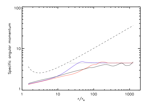
Figure 1: The time evolution of the radial profile of the specific angular momentum of accretion flow at the equatorial plane (averaged from $\theta=84^{\circ}-96^{\circ}$) for model A. The dashed line shows the Keplerian angular momentum. The dotted line shows the initial angular momentum profile. The blue, red, and black lines show the angular momentum profiles at $t=0.03,0.3$ and 22, respectively.

Figure 2: The radial profile of the specific angular momentum of the accretion flow at the equatorial plane (averaged from $\theta=84^{\circ}-96^{\circ}$) for model B when a quasi-steady state is reached. Because the fluctuation in this model is much larger than that in model A, we use 50 data files cover 3 orbital times (from $t=13$ to 16) to average the data when drawing this figure. The dashed line shows the Keplerian angular momentum. The dotted line shows the initial angular momentum profile.

In our models, we set $l_{0}=l_{k}(20r_{s})$, here $l_{k}$ is the specific angular momentum. This means that if the “circularization radius” scenario is correct, we should expect that the accretion flow remains a constant angular momentum ($l_{0}$) outside of $20r_{s}$, they forms a Keplerian disk at $\sim 20r_{s}$. We now check whether this picture is true using simulations.

Fig. 1 shows the evolution of the radial profile of angular momentum for model A which uses the usual “$\alpha$”-viscosity description. The dotted, blue, red, and black solid lines show the profiles at time $t=0,0.03,0.3$ and $22$, respectively. At $t=22$, the accretion flow inside of $100r_{s}$ has achieved a steady state. From this figure, we can see that at the beginning of simulation, $t=0.03$, the profile of angular momentum does look like to be consistent with the “circularization” scenario, a “turning point” is evident in the blue solid line which reminds us the presence of the “circularization radius”. However, the profile quickly evolves with time. From the movie of evolution of accretion flow we make, we find that the “turning point” in the profile moves outward. Finally, when a steady state is reached, the profile is quite smooth throughout the whole region and the “turning point” completely disappears. The angular momentum at the outer region $r>1000r_{s}$ is larger than the initial value, this is because of the angular momentum transfer from small to large radii. Define the viscous time scale as $\tau_{v}=r^{2}/\nu$, we find that the time needed to achieve a state that the angular momentum is smooth throughout the flow is approximately $1/3$ times the viscous timescale at the Bondi radius.

We have tested whether the value of $\alpha$ and the r-dependence of viscosity affect our result by performing two test simulations. In the first test, we assume the r-dependence of viscosity is same as that in model A, but the value of $\alpha$ is five times smaller than that in model A. In the second test, we assume $\alpha$ is same as that in model A, but $\nu\propto r$. We find that the angular momentum profile in the two tests is very similar to that in model A when a steady state is achieved.

For model B, we have checked that in the quasi-steady state, our resolution in the inner region can resolve the fastest growth wavelength of MRI for the actual angular velocity profile and magnetic field strength. Fig. 2 shows the angular momentum profile for model B in the quasi-steady state. The evolution of the profile is similar to that shown in Fig. 1 and is not shown here. The angular momentum profile is very smooth in the region $r<300r_{s}$. The “turning point” moved to 300$r_{s}$ at the end of the simulation. It indicates that our simulation has not run enough time to reach a steady state at all radii. We expect that if we run the simulation for longer time, the “turning point” will move outward further until the angular momentum profile is smooth throughout the flow. In the region $r<6r_{s}$, the angular momentum decreases quickly inward. The reason is as follows. Inside $6r_{s}$, the magnetic field is very strong because of the accumulation of magnetic flux in the simulation (the magnetic pressure is actually higher than the gas pressure). Strong magnetic field results in strong Maxwell stress in this region which can transport the angular momentum very efficiently and makes the angular momentum inside $6r_{s}$ decreasing quickly inward.

We note that Proga & Begelman (2003) also studied the small angular momentum gas accretion. Although the profile of angular momentum is not explicitly shown in their paper, they do show that the rotational velocity profile. From their Fig. 9, it seems that there exists a “circularization radius”. We suspect that this is because they have not run the simulation for long enough time.

4 SUMMARY

A popular picture people have for the accretion of low-angular momentum flow is that a “circularization” radius should exist. Outside of this radius, the angular momentum of accretion flow is constant while inside of this radius the angular momentum roughly follow the Keplerian value thus a disk is formed. In this paper, by performing numerical simulations, we show that this picture is not correct. We find that for low angular momentum gas accretion, initially, there is a “turning point” at the “circularization” radius in the angular momentum distribution. But this “turning point” will move outward with time. The time needed to achieve a state that the angular momentum profile is smooth throughout the flow is approximately the viscous timescale at the outer boundary. Therefore, for an accretion system which can persist for a time that is longer than this timescale, the radial profile of the angular momentum will eventually become smooth throughout the accretion flow. On the other hand, we would like to emphasize that for transient accretion systems, such as the tidal disruption of a star by a black hole, the radial profile of the angular momentum should be smooth only inside a finite radius $R_{0}$, at which the viscous timescale equals the life time of the accretion event. Within this radius the specific angular momentum of the accretion flow is close to Keplerian or sub-Keplerian while beyond $R_{0}$ the angular momentum should roughly be constant.

In this picture, the angular momentum is significantly smaller than the Keplerian value, which implies that the gravitational force is larger than the centrifugal force. For a hot accretion flow, such a difference of force is balanced by the gradient of gas pressure. While for a cold accretion flow, the gradient of gas pressure may not be large enough to play such a role. In this case, perhaps it is the inertia force together with the centrifugal force that balances the gravitational force. Our simulation presented in this paper only holds for hot accretion flows. The simulation of cold accretion disk is technically difficult for us thus needs to be checked in the future.

References

- [] Abramowicz M. A., Zurek W. H., 1981, ApJ, 246, 314
- [] Abramowicz M. A., Chen X., Kato S., Lasota J. P., Regev O., 1995, ApJ, 438, L37
- [] Balbus S. A., Hawley J. F., 1991, ApJ, 376, 214
- [] Balbus S. A., Hawley J. F., 1998, Rev. Mod. Phys., 70,1
- [] Bu D. F., Yuan F., Wu M. C., Cuadra J., 2013, MNRAS, 434, 1692
- [] Gan Z. M., Yuan F. Ostriker, J. P. et al. 2014, submitted to ApJ (arXiv:1403.0670)
- [] Hirose S., Krolik J. H., Blaes O., 2009, ApJ, 691, 16
- [] Inogamov N. A., Sunyaev R. A., 2010, Astronomy Letters, Volume 36, Issue 12, pp.835-847
- [] Li J., Ostriker J., Sunyaev R., 2013, ApJ, 767,105L
- [] Melia,F., Liu, S., & Coker, R. 2001, ApJ, 553, 146
- [] Narayan R., Yi I., 1994, ApJ, 428, L13
- [] Narayan R., Yi I., 1995, ApJ, 452, 710
- [] Narayan R., Sadowski A., Penna R. F., Kulkarni A. K., 2012, MNRAS, 426, 3241
- [] Ostriker J. P., Choi E., Ciotti L, Novak G. S., Proga D., 2010, ApJ, 722, 642
- [] Proga D., Begelman M. C., 2003, ApJ, 592, 767
- [] Shakura N. I., Sunyaev R. A., 1973, A&A, 24, 337
- [] Stone J.M., Norman M. L., 1992a, ApJS, 80, 753
- [] Stone J.M., Norman M. L., 1992b, ApJS, 80, 791
- [] Stone J. M., Pringle J. E., 2001, MNRAS, 322, 461
- [] Stone J. M., Pringle J. E., Begelman M. C. 1999, MNRAS, 310, 1002
- [] Wang Q. D., Nowak M. A., Markoff S. B., et al., 2013, Science, 341, 981
- [] Xie F. G., Yuan F., 2012, MNRAS, 427, 1580
- [] Yuan F., 1999, ApJ, 521, L55
- [] Yuan F., Bu D., Wu M., 2012, ApJ, 761, 130
- [] Yuan F., Narayan R., 2014, ARA&A, in press (arXiv: 1401.0586)