Recovering rank-one matrices via rank-$r$ matrices relaxation

Abstract

PhaseLift, proposed by E.J. Candès et al., is one convex relaxation approach for phase retrieval. The relaxation enlarges the solution set from rank one matrices to positive semidefinite matrices. In this paper, a relaxation is employed to nonconvex alternating minimization methods to recover the rank-one matrices. A generic measurement matrix can be standardized to a matrix consisting of orthonormal columns. To recover the rank-one matrix, the standardized frames are used to select the matrix with the maximal leading eigenvalue among the rank-$r$ matrices. Empirical studies are conducted to validate the effectiveness of this relaxation approach. In the case of Gaussian random matrices with a sufficient number of nearly orthogonal sensing vectors, we show that the singular vector corresponding to the least singular value is close to the unknown signal, and thus it can be a good initialization for the nonconvex minimization algorithm.

1 Introduction

Phase retrieval is one important inverse problem that arises in various fields, including electron microscopy, crystallography, astronomy, and optics. [17, 14, 16, 19, 10, 9]. Phase retrieval aims to recover signals from magnitude measurements only (optical devices do not allow direct recording of the phase of the electromagnetic field).

Let $x_{0}\in\mathbf{R}^{n}$ or $x_{0}\in\mathbf{C}^{n}$ be some nonzero unknown vector to be measured. Let $A\in\mathbf{R}^{N\times n}$ be the matrix whose rows are sensing vectors $\{a_{i}\in\mathbf{R}^{n}\}_{i=1}^{N}$ or $\{a_{i}\in\mathbf{C}^{n}\}_{i=1}^{N}$. The measurement vector $b\in\mathbf{R}^{N}$ is the magnitude,

$$b=|Ax_{0}| b_{i}=|{a}_{i}\cdot x_{0}| i=1,\ldots,N$$, or for .

Obviously, the signal $x_{0}$ can be determined up to a global phase factor at best, i.e., becasue

$$|x_{0}\cdot a_{j}e^{i\theta}|=|x_{0}\cdot a_{j}|\textrm{ for any $\theta\in[0,2\pi]$},$$

then $x_{0}e^{i\theta}$ is also a solution. The recovery of $x_{0}e^{i\theta}$ is referred to as the exact recovery. When $A$ is a Fourier matrix, the problem is known as phase retrieval. With this specific measurement matrix, the task becomes more demanding, because Fourier magnitude is not only preserved under global phase shift, but also under spatial shift and conjugate inversion, which yields twin images[9].

The first widely accepted phase retrieval algorithm was presented by Gerchberg and Saxton[12]. Fienup[11] developed the convergence analysis of the error-reduction algorithm and proposed input-output iterative algorithms. The basic and hybrid input-output algorithms can be viewed as a nonconvex Dykstra algorithm and a nonconvex Douglas-Rachford algorithm, respectively[3]. Empirically, the hybrid input-output algorithm is observed to converge to a global minimum (no theoretical proof is available)[19].

The major obstacle to phase retrieval is caused by the lack of convexity of the magnitude constraint[9]. PhaseLift[6], proposed by E.J. Candès et al., is one convex relaxation approach for phase retrieval. The relaxation changes the problem of vector recovery into a rank-one matrix recovery. The global optimal solution can be achieved, when $A$ is a Gaussian random matrix and $N\geq Cn$ with some absolutely constant $C$[5]. To some extent, this approach provides a solution to the phase retrieval problem, at least from the theoretical perspective, provided that the feasible set can shrink to one single point under a sufficient number of measurements. In practice, the sensing matrix $A$ does not belong to this specific Gaussian model or uniform models, and the computational load of solving the convex feasibility problem can be too demanding. In particular, it requires the computation of all the singular values in each iteration.

In this paper, we explore the possibility of using the rank-$r$ matrix relaxation in phase retrieval. In the first section, to illustrate the idea, we review the exact recovery condition in PhaseLift. Typically, the exact recovery of rank-one matrices requires a large $N/n$ ratio. We standardize the frame, such that each matrix in the feasible set has an equal trace norm. Then, the desired rank one matrix is the matrix whose leading eigenvalue is maximized. Gradually enlarging the leading eigenvalue, the matrix moves towards the rank one matrix with high probability. Our simulation result substantiates the effectiveness of recovering rank one matrices.

To reduce the computational load, in section 2, we apply the relaxation to the nonconvex alternating direction minimization method (ADM) proposed in [22]. Frames are standardized to ensure the equal trace among all feasible solutions. In theory, searching for the optimal solution in a higher dimensional space can alleviate the stagnation of local optima. Finally, with a sufficient amount of nearly orthogonal sensing vectors, we show that the corresponding singular vector is close to the unknown signal and can thus be a good initialization. To some extent, this theoretical result provides a partial answer to the solvability of phase retrieval. In fact, when there is a lack of nearly orthogonal sensing vectors, the ADM can fail to converge, as discussed in Section 3.1.

In section 3, we conduct a few experiments to demonstrate the performance of the ADM methods, including the convergence failure of nonconvex ADM, the comparison between rank one ADM to rank-$r$ ADM, and the application of phase retrieval computer simulations. Finally, given a generic matrix, we can find an equivalent matrix whose columns are orthogonal and whose rows have equal norm. We discuss the existence and uniqueness proof of the orthogonal factorization in the appendix.

1.1 Notation

In this paper, we use the following notations. Let $x^{\top}$ be the Hermitian conjugate of $x$, where $x$ can be real or complex matrices (or vectors). Hence, $x$ is Hermitian if $x=x^{\top}$. The notation $x^{*}$ is reserved for a limit point of a sequence $\{x^{k}\}_{k=0}^{\infty}$ or the final iteration of $x$ in the computation. Let $\|x\|_{F}$ be the Frobenius norm. The function $diag(X)$ produces a vector that is the diagonal of a matrix $X$. The pseudo-inverse of matrix $X$ is denoted by $X^{\dagger}$. The vector $e$ is a vector consisting of one, and $e_{j}$ is the vector consisting of zero, except one at the $j^{th}$ entry. Let $x_{0}\in\mathbf{R}^{n}$ be the unknown signal and $A\in\mathbf{R}^{N\times n}$ or $\in\mathbf{C}^{N\times n}$ be the sensing matrix. Hence $N$ is the number of measurements.

1.2 Ratio $N/n$

We shall briefly outline the threshold ratio $N/n$ on the exact recovery of $x_{0}$ [1]. The result can be regarded as a worst-case bound, because we demand the exact recovery for all possible nonzero vectors $x$. Denote a nonlinear map associated with $A$ by $M^{A}:\mathbf{R}^{n}\to\mathbf{R}^{N}$,

$$M^{A}(x)=\sum_{k=1}^{N}|a_{k}\cdot x|e_{k}.$$

The range of the mapping $M^{A}$ consists of all the possible measurement vectors $b$ via the sensing matrix $A$.

Throughout this paper, we assume that $A$ has rank $n$. We say that a matrix $A\in\mathbf{R}^{N\times n}$ satisfies the rank* condition if all square $n$-by-$n$ sub-matrices of $A$ has full rank and $N>n$. That is, any $n$ row vectors of $A$ are linearly independent.

Proposition 1.1.

Suppose that $A$ satisfies the rank* condition. If $N\geq 2n-1$, then $M^{A}:\mathbf{R}^{n}\to\mathbf{R}^{N}$ is injective.

Proof.

Suppose that $M^{A}(x)=M^{A}(\hat{x})$ with $x\neq\hat{x}$; then $|a_{k}\cdot x|=|a_{k}\cdot\hat{x}|$. Rearrange the indices and assume

$$a_{k}\cdot x=a_{k}\cdot\hat{x}\textrm{ for }k=1,\ldots,l,$$

$$a_{k}\cdot x=-a_{k}\cdot\hat{x}\textrm{ for }k=l+1,\ldots,N.$$

Because $N\geq 2n-1$, then either $l\geq n$ or $N-l\geq n$. Suppose $l\geq n$. Then $x-\hat{x}\in\mathbf{R}^{n}$ is orthogonal to $a_{1},\ldots,a_{l}$. The full rank condition yields $x-\hat{x}=0$, which shows the nonexistence of two distinct vectors $x,\hat{x}$. Similar arguments apply to the case $N-l\geq n$. ∎

According to the above proof, when $N\leq 2n-2$, we can find a pair of vectors $x,\hat{x}$ such that $|Ax|=b=|A\hat{x}|$. Indeed, when $N=2n-2$, let $u$ be the vector orthogonal to $\{a_{i}\}_{i=1}^{n-1}$ and $v$ be the vector orthogonal to $\{a_{i}\}_{i=n}^{2n-2}$. Then $x=u+v$ and $\hat{x}=u-v$ are the desired pair of vectors. However, for any particular vector $x$, it is possible that no $\hat{x}\in\mathbf{R}^{n}$ exists in the case $n+1\leq N\leq 2n-2$.

Proposition 1.2.

Fix $x_{0}\in\mathbf{R}^{n}$. Suppose each row $a_{i}$ of $A$ is independently sampled from some continuous distribution on the unit sphere in $\mathbf{R}^{n}$. Let $b=|Ax_{0}|$. Then, with probability one, $|Ax|=b$ has a unique solution $x=x_{0}$ for $N\geq n+1$.

Proof.

Assume $N=n+1$. Write

$$A:=\left[\begin{array}[]{c}A_{1}\\ A_{2}\end{array}\right]\textrm{ with }A_{1}\in\mathbf{R}^{n,n},A_{2}\in\mathbf{R}^{1,n}.$$

Then with probability one, $A_{1}$ is full rank and thus we can find a unique nonzero vector $c\in\mathbf{R}^{n}$ such that $a_{n+1}=c^{\top}A_{1}$. Clearly, $c$ is a continuous random vector that depends on $A_{2}$.

Suppose that $x=\hat{x}$ is another solution of $|Ax|=b$. Then $\hat{x}$ should be one solution of $2^{n}$ possible systems

$$\{(A_{1}\hat{x})_{i}=\pm b_{i}\}\textrm{ for $i=1,\ldots,n$.}$$

Let $y:=A_{1}(x_{0}\pm\hat{x})$. Then, $y$ must be one of the $3^{n}$ vectors with $y_{i}=\pm 2b_{i}$ or $0$ for $i=1,\ldots,n$. Note that $y$ is independent of the selection of $A_{2}$. Alternatively, $a_{n+1}x_{0}=\mp a_{n+1}\hat{x}$ yields the orthogonality between $c$ and $A_{1}(x_{0}\pm\hat{x})$, i.e.,

$$a_{n+1}\cdot(x_{0}\pm\hat{x})=c^{\top}A_{1}(x_{0}\pm\hat{x})=c\cdot y=0.$$

Since $c$ is a continuous random vector that depends on $A_{2}$, then with probability one, $c\cdot y=0$ leads to $y=0$, which implies that $x=\pm\hat{x}$ ($A_{1}$ is full rank). ∎

However, for generic complex frames, the map is injective if $N\geq 4n-2$, i.e., all vectors $x_{0}\in\mathbf{C}^{n}$ can be recovered. To recover a fixed vector $x_{0}$, $N\geq 2n$ is a necessary condition. Interested readers are referred to the discussion in [1] and [2].

One naive thought is that as $N$ grows faster than the speed of $n$, the rank one matrix can be recovered. Unfortunately, this can be incorrect in some circumstances. We can construct some matrix $A\in\mathbf{R}^{N\times n}$ with $N$ being order of $2^{n}$, but some vector $x_{0}$ still cannot be recovered due to the failure of the rank* condition, see the following remark.

Remark 1.3.

(Bernoulli random matrices) We construct an example, in which $x_{0}=e_{1}$ cannot be recovered from the measurement $|Ax_{0}|=b=e$. Denote by $S\subset\mathbf{R}^{n}$ a set of vectors whose entries are $\pm 1$. There are $2^{n}$ vectors in $S$. Pick any subset of $N$ vectors from $S$ as $\{a_{i}\}_{i=1}^{N}$ ($A\in\mathbf{R}^{N\times n}$ is the Bernoulli random matrix). All the vectors $e_{j},j=1,\ldots,n$ satisfy $|Ae_{j}|=|Ax_{0}|=b=e$. Since these matrices are indistinguishable, $M^{A}$ does not the injective property. Note that the rank of the random matrix $A$ is $n$ in most cases. The rank $n$ condition on $A$, together with a large $N$, does not imply the exact recovery of $x_{0}$. One can easily verify that the Fourier matrix yields the same difficulty.

1.3 PhaseLift

Next, we introduce the PhaseLift method proposed by Candès et al.[6]. To simplify the discussion, we focus on the noiseless case. Introduce the linear operator on Hermitian matrices,

$$\mathcal{A}:\mathcal{H}^{n\times n}\to\mathcal{R}^{N},\;\mathcal{A}(X):=diag(A^{\top}XA)=b^{2},\;b_{i}^{2}=a_{i}^{\top}Xa_{i},i=1,\ldots,N.$$

An equivalent condition of $|Ax_{0}|=b$ is that $X:=x_{0}x_{0}^{\top}$ is a rank-one solution to $\mathcal{A}(X)=b^{2}$. Hence, the phase retrieval problem can be formulated as the matrix recovery problem,

$$\min_{X}rank(X)\textrm{ subject to }\mathcal{A}(X)=b^{2},X\succeq 0.$$

By factorizing a rank one solution of $X$, we can recover the signal $x_{0}$.

To overcome the difficulty of rank minimization, Candès et al. [6] propose a convex relaxation of the rank minimization problem, which is the trace minimization problem,

$$\min_{X}tr(X),\textrm{ subject to }\mathcal{A}(X)=b^{2},X\succeq 0.$$

When

$$I_{n\times n}\in span\{a_{i}a_{i}^{\top}\}_{i=1}^{n},$$

the condition $\mathcal{A}(X)_{i}=tr(a_{i}a_{i}^{\top}X)$ automatically determines the trace $tr(X)$ of $X$ and then the trace minimization objective is redundant. Recovering $X_{0}=x_{0}x_{0}^{\top}$ can be achieved via solving the following convex feasibility problem,

$$\{X:X\succeq 0,\mathcal{A}(X)=b^{2}\}.$$ (1.1)

In the next subsection, we will show that we can always remove the trace minimization objective via an orthogonal decomposition on $A$, either SVD or QR factorizations.

The following Prop. [6] illustrates the optimality of the feasibility problem, which is a key tool for justifying the exact recovery theoretically. The proof can be found in [8].

Proposition 1.4.

Suppose that the restriction of $\mathcal{A}$ to the tangent space at $X_{0}:=x_{0}x_{0}^{\top}$ is injective. One sufficient condition for the exact recovery is the existence of $y\in\mathbf{R}^{N}$, such that

$$Y:=\mathcal{A}^{\top}y=A^{\top}diag(y)A=\sum_{i=1}^{N}y_{i}a_{i}a_{i}^{\top}$$

satisfies

$$Y_{T}=0\textrm{ and }Y_{T^{\bot}}\succ 0.$$

The proposition states one sufficient condition under which $x_{0}x_{0}^{\top}$ can be recovered from the frame $A$. In the real case, when $N\geq 2n-1$, the rank* condition on $A$ is one sufficient condition to ensure the injective property of the restriction of $\mathcal{A}$. Indeed, for any $x_{0}\neq 0$, $Ax_{0}$ consists of at most $n-1$ zeros thanks to the rank* condition, thus $Ax_{0}$ consists of at least $n$ nonzero entries. Since the tangent space at $x_{0}x_{0}^{\top}$ consists of $\hat{X}$ in a form $x_{0}x^{\top}+xx_{0}^{\top}$ with some $x\in\mathbf{R}^{n}$, then

$$\mathcal{A}(\hat{X})=\mathcal{A}(x_{0}x^{\top}+xx_{0}^{\top})=2(Ax_{0})(Ax)=0\in\mathbf{R}^{N}$$

yields $x=0$ (due to the rank* condition), which implies $\hat{X}=0$.

1.4 Special frames

We shall highlight three special frames where the feasible set only consists of one single point. Thus the unknown signal $x_{0}$ can be recovered via PhaseLift. In the first case, we show that a frame with $N=n+1$ measurement vectors are sufficient to determine the unknown matrix $X=x_{0}x_{0}^{\top}$.

Proposition 1.5.

Suppose that $a_{j}=e_{j}$ for $j=1,\ldots,n$ and $a_{n+1}(j)x_{0}(j)>0$ for $j=1,\ldots,n$. Then, the feasible set of PhaseLift consists of only one single point, $x_{0}x_{0}^{\top}$.

Proof.

From $a_{j}=e_{j}$, we have

$$a_{j}^{\top}Xa_{j}=X_{j,j}=|x_{0}(j)|^{2}.$$

The positive semidefinite requirement of $X$ yields $X_{i,j}^{2}\leq X_{i,i}X_{j,j}$. The measurement $a_{n+1}^{\top}Xa_{n+1}=|a_{n+1}\cdot x_{0}|^{2}$ enforces $a_{n+1}^{\top}Xa_{n+1}$ to reach its upper bound among $X$ being positive semidefinite, i.e., the inequalities in the following relation become equalities,

$$a_{n+1}^{\top}Xa_{n+1}=\sum_{i,j}a_{n+1}(i)X_{i,j}a_{n+1}(j)$$

$$\leq\sum_{i,j}|a_{n+1}(i)a_{n+1}(j)|\sqrt{X_{i,i}}\sqrt{X_{j,j}}\leq(\sum_{j}|a_{n+1}(j)|\sqrt{X_{j,j}})^{2}=|a_{n+1}\cdot x_{0}|^{2},$$

where we used the assumption $a_{n+1}(j)x_{0}(j)>0$ for all $j=1,\ldots,n$. Hence, $X_{i,j}^{2}=X_{i,i}X_{j,j}$ for all $i,j$, which implies $X=xx^{\top}$ is the only feasible point with $x:=(a_{n+1}x_{0}/|a_{n+1}|)$.

∎

In the second case, the exact recovery is obtained via a set of sensing vectors orthogonal to $x_{0}$.

Proposition 1.6.

Suppose that some $n-1$ linear independent sensing vectors among $\{a_{i}\}_{i=1}^{n}$ exist such that $x_{0}\cdot a_{i}=0$; then, PhaseLift with measurement matrix $A$ recovers the matrix $x_{0}x_{0}^{\top}$ exactly.

Proof.

Without loss of generality, assume that $x_{0}=e_{1}$ and write $A$ as an $n\times n$ matrix,

$$A=\left(\begin{array}[]{cc}1_{1\times 1}&*_{1\times(n-1)}\\ 0_{(n-1)\times 1}&A_{1}\end{array}\right)$$

where $A_{1}\in\mathbf{R}^{(n-1)\times(n-1)}$ has rank $n-1$, i.e., it consists of linear independent columns. Choose $y$ to be a vector with $y_{i}>0$ for $i\geq 2$. Then $Y_{T}=0$ and for any $z\in\mathbf{R}^{n-1}$,

$$(A_{1}z)^{\top}diag([y_{2},\ldots,y_{n}])A_{1}z=0.$$

Because $y_{i}>0$ for all $i=2,\ldots,n$, then $A_{1}z=0,\;i.e.,z=0.$ Hence, $Y_{T^{\bot}}\succ 0$. ∎

This special choice of the first column of $A$ indicates the orthogonality between $n-1$ sensing vectors $a_{i}$ and $x_{0}$. However, the orthogonality is generally not satisfied for arbitrary vector $x_{0}$.

In the third case, the exact recovery can be obtained via some structured sensing matrix, which in fact fails the rank* condition ($M^{A}$ is not injective).

Proposition 1.7.

Suppose that $N=2n-1$ and the sensing vectors in $A$ are $a_{i}=e_{i}$ for $i=1,\ldots,n$ and

$$a_{n+i}=e_{i}+\beta_{i}e_{i+1} \beta_{i}\neq 0 i=1,\ldots,n-1$$ with for .

Suppose that the entries of $x_{0}$ are nonzero. Then PhaseLift with measurement matrix $A$ recovers the matrix $x_{0}x_{0}^{\top}$ exactly.

Proof.

To simplify the discussion, assume $x_{0}=e$ and replace vectors $a_{i}$ with vectors $a_{i}x_{0}$ for all $i$. Any matrix $X$ in the feasible set has the form,

$$X\in\mathbf{R}^{n,n}=\left(\begin{array}[]{ccccc}1&1&&&\\ 1&1&1&&\\ &1&1&1&\\ &&&\ldots&\\ &&&1&1\end{array}\right),$$

i.e., $X_{i,i+1}=X_{i,i}=X_{i+1,i}=1$.

Claim: Because $X$ is positive semidefinite, any principal sub-matrices of $X$ are positive semidefinite, which implies that $X=ee^{\top}$.
Start with $\alpha:=X_{i_{1},j_{1}}=X_{j_{1},i_{1}}$ with $i_{1}=j_{1}+2$. Consider the principal sub-matrix $\{X_{i,j}:i,j\in\{j_{1},j_{1}+1,j_{1}+2\}\}$. Compute the determinant of this submatrix

$$-1+2\alpha-\alpha^{2}=-(1-\alpha)^{2}.$$

Hence, the nonnegative determinant yields $\alpha=1$. Similar arguments work for $i_{1}=j_{1}+3$,…. In the end, all entries of $X$ must be $1$, i.e., $X=x_{0}x_{0}^{\top}$ is the only matrix in the feasible set. ∎

Readers can apply the similar arguments to the recovery of $X_{0}=x_{0}x_{0}^{\top}$ with $x_{0}\in\mathbf{C}^{n}$ via the following matrix: Let $A\in\mathbf{C}^{N,n}$ with $N=n+2(n-1)$ and

$$a_{i}=e_{i},\;a_{n+i}=e_{i}+\beta_{i}e_{i+1},\textrm{ and $a_{2n-1+i}=e_{i}+\gamma_{i}e_{i+1}$, where }$$

$$\textrm{ $\beta_{i}\neq\gamma_{i}$ are nonzero for $i=1,\ldots,n-1$}.$$

See [4] for more discussion on the usage of $N=3n-2$ sensing vectors.

1.5 Reduction of $N/n$ via standardized frames

In the following, some orthogonality on $A$, $A^{\top}A=I_{n\times n}$ is expected to implement the matrix recovery algorithm. We say that a measurement matrix (a frame) $A$ is standardized if $A$ consists of orthonormal columns, i.e., $A^{\top}A=I_{n\times n}$. In fact, given any measurement matrix $A\in\mathbf{R}^{N\times n}$ with rank $n$, we can take the QR decomposition of the measurement matrix $A$, $A=QR$ with $Q\in\mathbf{R}^{N\times n}$ consisting of orthonormal columns and $R\in\mathbf{R}^{n\times n}$ being upper triangular. The rank of $A$ is equal to the rank of $R$. Hence, denoting $Rx$ by $y$, the problem is reduced to solving $y$ from the measurements

$$|Ax|=|QRx|=|Qy|=b.$$

Once $y$ is obtained, $x$ can be computed via simply inverting the matrix $R$. Hence, the original frame $A$ is equivalent to the standardized frame $Q$ in the sense that the two transforms $A,Q$ have the same range. That is, $M^{A}$ is injective if and only if $M^{Q}$ is injective.

In the section, we propose one modification on PhaseLift to recover the rank one matrix $X_{0}$. The idea is based on the following simple fact. Among the feasible set $\mathcal{A}(X)=b^{2}$ and $X$ being positive semidefinite, to recover the rank one solution, we should choose the matrix $X$ whose leading eigenvalue is maximized.

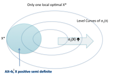
(a) One optimal solution

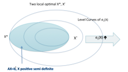
(b) Two optimal solutions

Figure 1: Maximizing the leading eigenvalue yields the rank one solution.

Consider the model

$$\min_{X}-\sigma_{1}(X),$$

subject to $X$ positive semidefinite and $\mathcal{A}X=b^{2}$, where $\sigma_{1}(X)$ refers to the largest eigenvalue function of $X$. See Fig. 1.

Then we have the following theoretical result.

Theorem 1.8.

Suppose that $A$ is a standardized matrix with $N\geq 2n-1$ in the real case and $N\geq 4n-2$ in the complex case. Then with probability one, the global minimum occurs if and only if the minimizer $X$ is exactly $X=x_{0}x_{0}^{\top}$.

Proof.

Because $|Ax|^{2}=b^{2}$ and $A$ consists of orthogonal columns,

$$e\cdot b^{2}=tr(X)=\sum_{i=1}^{n}\sigma_{i}(X),$$

where $\sigma_{i}(X)$ refers to the $i$-th eigevlaue of $X$. Because $X$ is positive semidefinite, the largest eigenvalue of $X$, which cannot exceed $e\cdot b^{2}$, is maximized if and only if $X$ is a rank one matrix. Finally, according to the above results, when $N$ exceeds the thresholds $2n-1$ or $4n-2$, with probability one, the rank one matrix is unique, which completes the proof. ∎

To address the problem, we propose the following alternating direction method(ADM). The ADM can be formulated as

$$\min_{X,Y}L_{\beta}(X,Y,\lambda):=-\sigma_{1}(X)-\lambda(X-Y)+\beta\|X-Y\|_{F}^{2}/2,$$

subject to $X$ positive semidefinite and $\mathcal{A}Y=b$. Hence, the update of $X,Y$ is

$$arg\min_{X}-\sigma_{1}(X)+\beta\|X-Y-\lambda/\beta\|_{F}^{2}/2\textrm{ subject to positive semidefinite,}$$ (1.2)

$$arg\min_{Y}\beta\|X-Y-\lambda/\beta\|_{F}^{2}/2\textrm{ subject to $\mathcal{A}Y=b^{2}$}.$$

The iteration becomes

1. Update $X$: Write $Y^{k}=UD_{Y}U^{\top}$; then, thanks to the rotational invariance of Frobenius norm, the minimizer in Eq. (1.2) is

   $$X^{k+1}=UD_{X}U^{\top},\textrm{ where }\;D_{X}=\max(D_{Y+\lambda/\beta},0)+\beta^{-1}e_{1}e_{1}^{\top},$$

   where $D_{Y+\lambda/\beta}$ is the diagonal matrix of the eigenvalue decomposition of $Y^{k}+\lambda^{k}/\beta$ and the diagonal entries are in a decreasing order, i.e., the $(1,1)$ entry is the largest eigenvalue and will be added by $\beta^{-1}$ in the $X$ update.

2. Update $Y$ via the projection of $X-\lambda/\beta$,

   $$Y^{k+1}=\mathcal{A}^{\top}(\mathcal{A}\mathcal{A}^{\top})^{-1}b+(I-\mathcal{A}^{\top}(\mathcal{A}\mathcal{A}^{\top})^{-1}\mathcal{A})Z,\textrm{ where }Z=X^{k+1}-\lambda^{k}/\beta.$$

   The matrix $\mathcal{A}^{\top}(\mathcal{A}\mathcal{A}^{\top})^{-1}\mathcal{A}$ is the orthogonal projector onto $Range(\mathcal{A}^{\top})$ which is spanned by $\{a_{i}a_{i}^{\top}\}_{i=1}^{N}$, each of which has trace one.

3. Update $\lambda$:

   $$\lambda^{k+1}=\lambda^{k}-\beta(X^{k+1}-Y^{k+1}).$$

Remark 1.9 (Counterexamples).

Because $\sigma_{1}(X)$ is convex in $X$, minimizing $-\sigma_{1}(X)$ yields a non convex minimization problem. Theoretically, there is no guarantee that the global optimal solution can always be found numerically; however, the empirical study shows that the exact recovery will occur with high probability.

Here is one counterexample.

$$A=\left(\begin{array}[]{ccc}1&1&1\\ 1&-1&-1\\ 1&\sqrt{3/2}&0\\ 1&-\sqrt{3/2}&0\\ 1&0&\sqrt{3}\\ 1&0&-\sqrt{3}\end{array}\right)$$

Then the feasible set consists of matrices $\left(\begin{array}[]{ccc}1-3\mu&0&0\\ 0&2\mu&0\\ 0&0&\mu\end{array}\right)$ with $\mu\in[0,1/3)$. The maximization of the leading eigenvalue leads to two possible solutions to $|Ax|^{2}=b^{2}$: one is $\mu=0$ (the rank-one solution) and the other is $\mu=1/3$ (the rank-two solution), depending on the initialization. See Fig. 2.

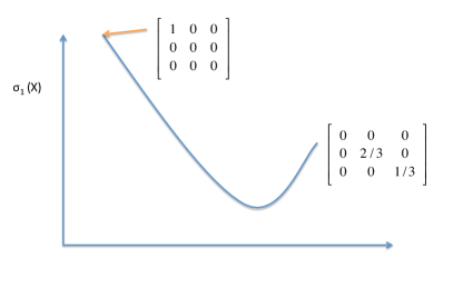
Figure 2: Maximizing the leading eigenvalue $\sigma_{1}(X)$ yields two local optimal solutions.

The following experiments illustrate that when the ratio $N/n$ is not large enough, the solution in PhaseLift is not rank one; we can successfully recover the rank one matrices via maximizing the leading eigenvalue; see Table 1 for the real case and Table 2 for the complex case.

Table 1: The number of successes out of $50$ random trials with $N=2n-1$. “via Q” refers to the standardized measurement.

n	PhaseLift		$\min-\sigma_{1}(X)$
	via $A$	via $Q$	via $A$	via $Q$
5	37	38	13	50
10	28	31	11	49
15	17	21	13	47
20	16	25	15	48
25	10	13	4	48
30	3	7	13	48
35	3	4	16	47
40	1	5	6	46
45	0	0	4	48
50	0	0	12	50

Table 2: The number of successes out of $20$ random trials via $N=2n-1,3n-1,4n-2$ standardized measurements ( complex case).

n	N=2n-1	N=3n-1	N=4n-2
5	3	20	20
10	2	20	20
15	1	20	20
20	0	20	20
25	0	20	20
30	0	20	20
35	0	20	20
40	0	20	20
45	0	20	20
50	0	20	20

The result of nonconvex minimization depends on the choice of initialization for $X^{0}$. When $X^{0}$ is near $X_{0}$, the exact recovery can be obtained.

Proposition 1.10.

Let $X_{0}=x_{0}x_{0}^{\top}$. Let $X$ be some positive semidefinite matrix. Let $f(t)$ be the spectral norm of matrices $tX_{0}+(1-t)X$,

$$f(t)=\|tX_{0}+(1-t)X\|,\;0\leq t\leq 1.$$

Let $v_{1}$ be the unit eigenvector corresponding to the largest eigenvalue of $X$. If $tr(X_{0}v_{1}v_{1}^{\top})\geq\|X\|$, then $f(t)$ increases on the interval $[0,1]$. Hence, $\min(-\sigma_{1}(X))$ yields the recovery of $X_{0}$.

Proof.

Observe that $f(t)$ is convex in $t\in[0,1]$. It suffices to show that $f(t)\geq f(0)$ for $t\in(0,1)$. According to the subdifferential of the matrix spectral norm[21], we have

$$t^{-1}(f(t)-f(0))\geq tr((X_{0}-X)^{\top}G),$$

where $G$ is a subgradient of the spectral norm at $X$. Choose $G=v_{1}v_{1}^{\top}$, then we have $tr((X_{0}-X)^{\top}G)=tr(X_{0}v_{1}v_{1}^{\top})-f(0)$, which completes the proof. ∎

Remark 1.11.

We provide a few examples to illustrate the recovery of $X_{0}$ via $-\min\sigma_{1}(X)$. Let $x_{0}=e\in\mathbf{R}^{3}$ and $X_{0}=ee^{\top}\in\mathbf{R}^{3\times 3}$. Suppose $a_{1}=e_{1}$, $a_{2}=e_{2}$ and $a_{3}=e_{3}$. Then, any feasible matrix has the form

$$X=\left(\begin{array}[]{ccc}1&1-\alpha_{1}&1-\alpha_{2}\\ 1-\alpha_{1}&1&1-\alpha_{3}\\ 1-\alpha_{2}&1-\alpha_{3}&1\end{array}\right)\textrm{ with }\alpha_{i}\geq 0.$$

Consider the case $\alpha_{1}=\alpha_{2}=\alpha$ and $\alpha_{3}=\alpha t$, then denote

$$X_{\alpha,t}:=\left(\begin{array}[]{ccc}1&1-\alpha&1-\alpha\\ 1-\alpha&1&1-\alpha t\\ 1-\alpha&1-\alpha t&1\end{array}\right),$$ (1.3)

and

$$\det(X_{\alpha,t})=\alpha^{2}t(4-2\alpha-t).$$

Thus, $X_{\alpha,t}$ is positive semidefinite if and only if

$$0\leq t\leq 4-2\alpha 0\leq\alpha\leq 2$$ and .

Hence, $X_{\alpha,4-2\alpha}$ has two positive eigenvalues and one zero eigenvalue if $0<\alpha<2$. For instance, when $\alpha=1/2$ and $t=3$, $X_{\alpha,t}$ has eigenvalues $1.5,1.5,0$. From the previous proposition, a positive semidefinite matrix $X_{\alpha,t}$ with $0\leq\alpha\leq 1/2$ can return to $X_{0}$ via maximizing the leading eigenvalue. See Fig. 3.

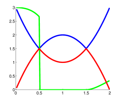
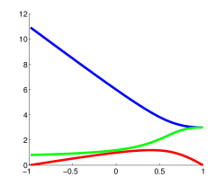
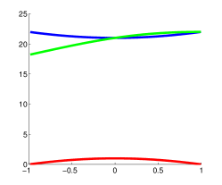
Figure 3: The left subfigure shows $\sigma_{1}(X_{\alpha,4-2\alpha})$ (blue), $\sigma_{2}(X_{\alpha,4-2\alpha})$ (red) and $|x_{0}\cdot v_{1}|^{2}$ (green). The middle and right subfigures show the results of $X_{\alpha,2\alpha-1}$ in Eq. (1.5) and $X_{\alpha}$ in Eq. (1.7), respectively. The x-axis represents $\alpha$ values.

The next example illustrates the necessity of trace invariance in recovering $X_{0}$. When the matrix trace is not constant in the feasible set, then maximizing the leading eigenvalue does not recover $X_{0}$ in general. For instance, consider$X_{0}=x_{0}x_{0}^{\top}$ with $x_{0}=e=[1,1,1]^{\top}$, and

$$A=\left(\begin{array}[]{ccc}1&0&1\\ 0&1&0\\ 0&0&1\\ 1&1&2\end{array}\right),\;b=|Ae|=\left(\begin{array}[]{c}2\\ 1\\ 1\\ 4\end{array}\right).$$

Any matrix $X$ in the feasible set has the form

$$X_{\alpha,\beta}:=\left(\begin{array}[]{ccc}3-2\beta&\beta&2-\alpha\\ \beta&1&\alpha\\ 2-\alpha&\alpha&1\end{array}\right)\textrm{ with }\det(X_{\alpha,\beta})=-(2\alpha-\beta-1)^{2},$$ (1.4)

and thus $\det(X_{\alpha,\beta})\geq 0$ yields $\beta=2\alpha-1$. In fact, the feasible set consists of matrices

$$X_{\alpha,2\alpha-1}=(1-t)\hat{e}\hat{e}^{\top}+tee^{\top},\hat{e}=[3,1,1]^{\top},\;t=(\alpha+1)/2\in[0,1].$$ (1.5)

Maximizing the leading eigenvalue yields the solution $e\hat{e}$, which is not $X_{0}$. Alternatively, consider the QR factorization,

$$A=QR=\left(\begin{array}[]{ccc}1/\sqrt{2}&0&-1/\sqrt{3}\\ 0&1&0\\ 0&0&1/\sqrt{3}\\ 1/\sqrt{2}&0&1/\sqrt{3}\end{array}\right)\left(\begin{array}[]{ccc}\sqrt{2}&\sqrt{2}&\sqrt{2}\\ 0&1&0\\ 0&0&\sqrt{3}\end{array}\right),$$

which yields the problem instead,

$$b=|QRe|=|Qx_{0}|,\;x_{0}:=Re=\left(\begin{array}[]{c}3\sqrt{2}\\ 1\\ \sqrt{3}\end{array}\right).$$

Then the feasible set $\{X:diag(QXQ^{\top})=b^{2},X\succeq 0\}$ consists of

$$X_{\alpha}:=\left(\begin{array}[]{ccc}18&3\sqrt{2}\alpha&3\sqrt{6}\\ 3\sqrt{2}\alpha&1&\sqrt{3}\alpha\\ 3\sqrt{6}&\sqrt{3}\alpha&3\end{array}\right),\;\alpha\in\mathbf{R}.$$ (1.6)

Let $x_{0}=[3\sqrt{2},-1,\sqrt{3}]^{\top}$ and $\hat{x}_{0}=[3\sqrt{2},-1,\sqrt{3}]^{\top}$. The feasible set consists of matrices

$$X_{\alpha}=(1-t)\hat{x}_{0}\hat{x}_{0}^{\top}+tx_{0}x_{0}^{\top},\;t=(\alpha+1)/2\in[0,1].$$ (1.7)

When $\alpha$ lies in $(0,1)$, maximizing the leading eigenvalue of $X_{\alpha}$ yields the exact recovery of $X_{0}$.

2 Low rank approaches

In PhaseLift, all eigenvalues of $X$ msy be computed in each iteration to be projected on the feasible set, consisting of positive semidefinite matrices with rank $n$. The projection obviously becomes a laborious task when $n$ is large. Here we propose to replace the feasible set with a subset consisting of rank-$r$ matrices, where $r$ is much smaller than $n$.

Write the positive semidefinite matrices $X$ in PhaseLift as $X=xx^{\top}$ with $x\in\mathbf{R}^{n,r}$ or $x\in\mathbf{C}^{n,r}$. Then, the original constraint in PhaseLift becomes

$$b^{2}=\mathcal{A}(X)=diag(AXA^{\top})=|Ax|^{2}.$$

2.1 ADM with $r=1$

Here we focus on the case $r=1$. In section 2.11, we will discuss the case $r>1$. When $r=1$, we arrive at the problem,

$$\textrm{ finding $x\in\mathbf{R}^{n}$ or $\mathbf{C}^{n}$ satisfying }|Ax|=b.$$

In [22], the framework

$$\min\frac{1}{2}\||z|-b\|^{2},\textrm{ subject to }z=Ax$$ (2.1)

is proposed to address phase retrieval. They introduce the augmented Lagrangian function

$$L(z,x,\lambda)=\frac{1}{2}\||z|-b\|^{2}+\lambda\cdot(Ax-z)+\frac{\beta}{2}\|Ax-z\|^{2}.$$ (2.2)

The algorithm consists of updating $z,x,$ and $\lambda$ as follows.

Algorithm 2.1.

Initialize $x^{0}$ randomly and $\hat{\lambda}^{0}=0$. Then repeat the steps for $k=0,1,2,\ldots$.

$$z^{k+1} = \frac{u}{|u|}\frac{b+\beta|u|}{1+\beta},\;u=Ax^{k}+\beta^{-1}\lambda^{k},$$

$$x^{k+1} = A^{\dagger}(z^{k+1}-\beta^{-1}\lambda^{k}),$$

$$\lambda^{k+1} = \lambda^{k}+\beta(Ax^{k+1}-z^{k+1}).$$

Let us simplify the algorithm. Let $P=AA^{\dagger}=QQ^{\top}$. Assume that $A$ has rank $n$. By eliminating $x^{k}$, the $\lambda$-iteration becomes

$$\beta^{-1}\lambda^{k+1}=(I-P)(\beta^{-1}\lambda^{k}-z^{k+1}).$$

Thus, $A^{\dagger}\lambda^{k+1}=0$. In the end, we have the following algorithm.

Algorithm 2.2.

Denote $\hat{\lambda}^{k}=\beta^{-1}\lambda^{k}$. Initialize $x^{0}$ randomly and $\hat{\lambda}^{0}=0$. Compute $z^{0}$. Then, repeat the steps for $k=0,1,2,\ldots$,

$$z^{k+1} = \frac{u}{|u|}\frac{b+\beta|u|}{1+\beta},\;u=Pz^{k}+\hat{\lambda}^{k},$$

$$\hat{\lambda}^{k+1} = (I-P)(\hat{\lambda}^{k}-z^{k+1}).$$

Remark 2.3 (Equivalence under right matrix multiplication).

Note that the iteration is updated via $P=QQ^{\top}$, instead of $A$. The matrix $R$ does not appear in the $z$ and $\lambda$ iterations. Thus, the algorithm is “ invariant” with respect to $R$. That is, for any invertible matrix $\hat{R}$, we get the same iterations $\{z^{k},\hat{\lambda}^{k}\}_{k=1}^{\infty}$, when $(A,x^{0})$ is replaced by

$$(Q\hat{R},(\hat{R})^{-1}Rx^{0}).$$

In particular, the iteration with $Q$ yields the same result as the one with $A$ itself. However, ADM can produce different results when the left matrix multiplication on $A$ is considered. See section 3.1.

Suppose that $z^{k}$ converges to $z^{*}$ and $\hat{\lambda}^{k}$ converges to $\hat{\lambda}^{*}$. Then, $Pz^{*}=z^{*}$ and $P\hat{\lambda}^{*}=0$. Hence, $x^{*}=A^{\dagger}z^{*}$, and $z^{*}=Pz^{*}=Ax^{*}$. Consider the limit of the $z$-iteration,

$$(1+\beta)z^{*}=\frac{u}{|u|}(b+\beta|u|)=\frac{u}{|u|}b+\beta(z^{*}+\hat{\lambda}^{*}).$$

Thus, we have the orthogonal projection of $bu/|u|$ onto the range of $A$ and its null space,

$$\frac{u}{|u|}b=z^{*}-\beta\hat{\lambda}^{*},$$

$$\textrm{ thus }\|b\|^{2}=\|z^{*}\|^{2}+\beta^{2}\|\hat{\lambda}^{*}\|^{2}.$$ (2.3)

This result shows $\|Ax^{*}\|\leq\|b\|$. In particular, when $A=Q$, we have $\|x^{*}\|\leq\|b\|=\|x_{0}\|$, i.e., any non-global solution has the smaller norm. Besides, Eq. (2.3) suggests the usage of smaller $\beta$ to improve the recovery of $x_{0}$. Empirical experiments show that, starting with $\lambda^{0}=0$, a smaller value $\beta$ leads to a higher chance of exact recovery.

To analyze the convergence, we write the function $L(z,x,\lambda)$ as

$$\hat{L}(z,x,\lambda,s):=\frac{1}{2}\|z-bs\|^{2}+\lambda\cdot(Ax-z)+\frac{\beta}{2}\|Ax-z\|^{2},$$

where the entries of $s$ satisfies $|s_{i}|=1$ for $i=1,\ldots,N$ and clearly the optimal vector $s$ to minimize $\hat{L}$ is given by $u/|u|$. When $s$ is fixed, then the following customized proximal point algorithm which consists of iterations

$$z^{k+1} = s\frac{b+\beta|u|}{1+\beta},\;u=Ax^{k}+\beta^{-1}\lambda^{k},$$

$$\lambda^{k+1} = \lambda^{k}+\beta(Ax^{k}-z^{k+1}),$$

$$x^{k+1} = A^{\dagger}(z^{k+1}-\beta^{-1}\lambda^{k+1})$$

can be used to solve the least squares problem

$$\min\frac{1}{2}\|z-sb\|^{2},\textrm{ subject to }z=Ax.$$ (2.4)

Gu et al. [13] provide the convergence analysis of the customized proximal point algorithm. More precisely, fixing $s$, let $(z^{*},x^{*},\lambda^{*})$ be a saddle point of $\hat{L}(z,x,\lambda,s)$ and let

$$\|v^{k+1}-v^{k}\|_{M}^{2}:=(v^{k+1}-v^{k})^{\top}M(v^{k+1}-v^{k})\textrm{ with }$$

$$M:=[\beta^{1/2}A,-\beta^{-1/2}I]^{\top}[\beta^{1/2}A,-\beta^{-1/2}I],\;v:=\left(\begin{array}[]{c}x\\ \lambda\end{array}\right).$$

In Lemma 4.2, Theorem 4.2 and Remark 7.1 [13], the sequence $\{v^{k}\}$ satisfies

$$\|v^{k+1}-v^{*}\|_{M}^{2}+\|v^{k}-v^{k+1}\|_{M}^{2}\leq\|v^{k}-v^{*}\|_{M}^{2},$$

and then $\lim_{k\to\infty}\|v^{k}-v^{k+1}\|_{M}^{2}=0$. Any limit point of $[z^{k},x^{k},\lambda^{k}]$ is a solution of the problem in Eq. (2.4) with $s$ fixed. However, the convergence analysis of the algorithm in Eq. (2.1) does not exist due to the lack of convexity in $z$. In fact, when $s$ is updated in each $z$-iteration, this algorithm sometimes fails to converge, which is shown in our simulations; see Section 3.1.

2.2 Recoverability

We make the following two observations regarding$|Ax_{0}|=b$. Suppose the unknown signal $x_{0}$ satisfies $\|x_{0}\|=1$. First, the vector $x$ is updated to maximize the inner product $|Ax|\cdot b$ in the ADM. However, because the norm constraint $\|x\|=1$ is not enforced explicitly, a non-global maximizer $x$ generally does not has the unit norm, $\|x\|<\|x_{0}\|=1$. In fact, classic phase retrieval algorithms e.g., ER, BIO, HIO[11], do not enforce the constraint directly. Second, for those indices $i$ with $a_{i}\cdot x$ close to zero, the unit vector $x$ to be recovered should be approximately perpendicular to these sensing vectors $a_{i}$. The candidate set $\{x:|a_{i}\cdot x|\leq b_{i}\}$ forms a cone, including unit vectors approximately orthogonal to $a_{i}$ corresponding to $b_{i}$ close to zero. In particular, when $a_{1}\cdot x_{0}\neq 0$ and $a_{i}\cdot x_{0}=0$ for $i=2,\ldots,N$ with $N>n$, then the cone is exactly the one-dimensional subspace spanned by the vector $x_{0}$.

One important issue of non-convex minimization problems is that the initialization can affect the performance dramatically. The x-iteration in the ADM tends to produce a vector close to the singular vector corresponding to its least singular value of $A$, in the sense that $A^{\dagger}z$ boosts the component along the singular vector corresponding to the largest singular value of $A^{\dagger}$, i.e., the smallest singular value of $A$. In the following, we will analyze the recovery problem from a viewpoint of singular vectors and derive an error estimate between the unknown signal and the singular vector.

Rearrange the indices such that $\{b_{i}\}$ are sorted in an increasing order,

$$0\leq b_{1}\leq b_{2}\leq\ldots\leq b_{N}.$$

Divide the indices into three groups,

$$\{1,2,\ldots,N\}=I\cup II\cup III.$$

We shall use subscripts $I,II,III$ to indicate the indices from these three groups. The set $I$ consists of the indices corresponding to the smallest $N_{I}$ terms among $\{b_{i}\}$. The set $II$ consists of the indices corresponding to the largest $N_{II}$ terms among $\{b_{i}\}$. Denote the matrix consisting of rows $\{a_{i}\}_{i\in I}$ by $A_{I}$. Let $A_{I}$ and $A_{II}$ consist of $N_{I}$ and $N_{II}$ rows, respectively. In the following, we illustrate that the singular vector $x_{min}$ corresponding to the least singular value of $A_{I}$ is a good initialization $x^{0}$ in the ADM.

Without loss of generality, assume that $x_{0}=e_{1}$ and that all the rows $\{a_{i}\}_{i=1}^{N}$ of $A$ are normalized, $\|a_{i}\|=1$. Observe that the desired vector satisfies $|Ax_{0}|\leq b$ and $\|x_{0}\|=1$. Hence, we look for a unit vector $x$ in the closed convex set

$$|a_{i}\cdot x|\leq b_{i}\textrm{ for all $i$}.$$

Whether phase retrieval can be solved depends on the structure of $A$. We make the following assumptions.

• First, sufficiently many indices $i\in I$ exist, such that

  $$\|b_{I}\|^{2}:=\sum_{i\in I}b_{i}^{2}\textrm{ is sufficiently small compared to }\|A_{I}x_{1}\|^{2},$$

  where $x_{1}$ is a unit vector orthogonal to $x_{0}$. (Clearly, the matrix $A_{I}$ has rank at least $n-1$.)

• Second, there are at least $n$ indices in $II$, such that

  $$\textrm{entries }\{b_{i}\}\textrm{ are {large} for }i\in II,$$

  and the matrix $A_{II}$ has rank $n$.

The assumption that $\{b_{i}\}_{i\in I}$ is close to zero implies that $\{a_{i}\}_{i\in I}$ are almost orthogonal to $x_{0}$. Thus, we instead solve the problem

$$\min_{x}\|A_{I}x\|^{2} \|x\|=1$$ with .

The minimizer denoted by $x_{min}$ is the singular vector $x_{min}$ corresponding to the least singular value of $A_{I}$. Then,

$$\|A_{I}x_{min}\|\leq\|b_{I}\|.$$

Let $\{0\leq\mu_{1}\leq\ldots\leq\mu_{n}\}_{i=1}^{n}$ be the singular values of $A_{I}$ with right singular vectors $v_{i}$. Then $v_{1}=\pm x_{min}$ and we can write

$$x_{0}=\alpha_{1}x_{min}+\sqrt{1-\alpha_{1}^{2}}\,w,$$

with some unit vector $w$ orthogonal to $x_{min}$. Let

$$x_{1}:=-(1-\alpha_{1}^{2})^{1/2}x_{min}+\alpha w,$$

then $x_{1}$ is a unit vector orthogonal to $x_{0}$. Note that

$$\|x_{0}x_{0}^{\top}-x_{min}x_{min}^{\top}\|^{2}=\|x_{0}x_{0}^{\top}-x_{min}x_{min}^{\top}\|^{2}_{F}/2=1-\alpha_{1}^{2}.$$

The following proposition gives a bound for the distance $\|x_{0}x_{0}^{\top}-x_{min}x_{min}^{\top}\|$ via the ratio $\|A_{I}x_{0}\|/\|A_{I}x_{1}\|$.

Proposition 2.4.

Let $\alpha_{1}=|x_{0}\cdot x_{min}|$. Then,

$$(2-\alpha_{1}^{2})\|b_{I}\|^{2}\geq(1-\alpha_{1}^{2})\|A_{I}x_{1}\|^{2}$$ (2.5)

Therefore, as $\|b_{I}\|$ is small enough, $1-\alpha_{1}^{2}$ must be close to $0$. Note that $\|b_{I}\|^{2}=\|A_{I}x_{0}\|^{2}$, then

$$\|b_{I}\|^{2}\|A_{I}x_{1}\|^{-2}\geq\left(\frac{1-\alpha_{1}^{2}}{2-\alpha_{1}^{2}}\right)\geq\frac{1}{2}\|x_{0}x_{0}^{\top}-x_{min}x_{min}^{\top}\|^{2}.$$ (2.6)

Proof.

Note that

$$\begin{cases}\|A_{I}x_{0}\|^{2}=\alpha_{1}^{2}\|A_{I}x_{min}\|^{2}+(1-\alpha_{1}^{2})\|A_{I}w\|^{2},\\ \|A_{I}x_{1}\|^{2}=(1-\alpha_{1}^{2})\|A_{I}x_{min}\|^{2}+\alpha_{1}^{2}\|A_{I}w\|^{2}.\;\end{cases}$$

Because $x_{min}$ is the singular vector of the the least eigenvalue,

$$(1-2\alpha_{1}^{2})\|A_{I}x_{0}\|^{2}-(1-\alpha_{1}^{2})\|A_{I}x_{1}\|^{2}$$

$$= \|A_{I}x_{min}\|^{2}+2(1-\alpha_{1}^{2})^{2}\left(\|A_{I}w\|^{2}-\|A_{I}x_{min}\|^{2}\right)\geq 0.$$

∎

Denote the sign vector of $A_{II}x_{min}$ by $u_{II}$,

$$u_{II}=\frac{A_{II}x_{min}}{|A_{II}x_{min}|}.$$

The closeness $\|A_{II}(x_{min}-x_{0})\|$ yields that $A_{II}x_{min}$ should be close to $A_{II}x_{0}$. In particular, when the magnitude of entries $b_{II}$ are large enough, both vectors have the same sign

$$\frac{A_{II}x_{min}}{|A_{II}x_{min}|}=\frac{A_{II}x_{0}}{|A_{II}x_{0}|}$$

and then

$$A_{II}x_{0}=u_{II}b_{II}.$$

Once the sign vector is retrieved, the vector $x_{0}$ can be computed via

$$x_{0}=A_{II}^{-1}(u_{II}b_{II}).$$

2.3 Real Gaussian matrices

As an example of computing $\|b_{I}\|$ and $\|A_{I}x_{1}\|$, let $A\in\mathbf{R}^{N\times n}$ be a random matrix consisting of i.i.d. normal $(0,1)$ entries. In the following, we would illustrate that when $N_{I}/N$ is small enough, $x_{min}$ is a good initialization for $x_{0}$ and thus we can recover the missing sign vector $(Ax_{0})/b$.

Let $x_{0}=e_{1}$. Then $x:=a_{i}\cdot x_{0}$ follows the distribution the normal $(0,1)$ distribution. Let $a>0$ be a function of $N_{I}/N$ and satisfy

$$F(a):=\int_{-a}^{a}(2\pi)^{-1/2}\exp(-x^{2}/2)dx=N_{I}/N.$$ (2.7)

Then the leading terms of Taylor series of Eq. (2.7) yields

$$(2/\pi)^{1/2}(a-a^{3}/6)\leq N_{I}/N\leq(2/\pi)^{1/2}a.$$ (2.8)

Define the “truncated” second moment

$$\sigma_{a}^{2}:=\int_{-a}^{a}x^{2}(2\pi)^{-1/2}\exp(-x^{2}/2)dx.$$

Taking the Taylor expansion of $\sigma_{a}^{2}$ in terms of $a$ yields the following result.

Proposition 2.5.

$$\sigma_{a}^{2}\leq(2/\pi)^{1/2}a^{3}/3.$$

Additionally, when $N_{I}/N$ tends to zero, $\sigma^{2}_{a}$ is approximately $(N_{I}/N)^{3}(\pi/6)$, where Eq. (2.8) is used.

When $N_{I}/N$ tends to zero, the following proposition shows that $N_{I}^{-1/2}\|b_{I}\|$ is approximately $(\pi/6)^{1/2}N_{I}/N$, see Fig. 4 for one numerical simulation.

Proposition 2.6.

Suppose $N_{I}/N<c$ for some constant $c$. Then with high probability

$$N_{I}^{-1/2}\|b_{I}\|\leq c_{6}(\pi/6)^{1/2}N_{I}/N,$$

for some constant $c_{6}$.

Proof.

Because $x_{0}=e_{1}$, $\|b_{I}\|$ is the norm of the first column of $A_{I}$. Let $\hat{\mu}>0$ be the sample $N_{I}$ quantile [7], $\hat{\mu}=|a_{N_{I}}\cdot x_{0}|$. We have the following probability inequality for $|\hat{\mu}-a|$: For every $\epsilon>0$,

$$\mathbb{P}(|\hat{\mu}-a|>\epsilon)\leq 2\exp(-2N\delta_{\epsilon}^{2})\textrm{ for all $N$,}$$

where

$$\delta_{\epsilon}:=\min\{F(a+\epsilon)-N_{I}/N,N_{I}/N-F(a-\epsilon)\}.$$

That is, with high probability we have

$$a-\epsilon\leq|a_{N_{I}}\cdot x_{0}|\leq a+\epsilon.$$ (2.9)

The proof is based on the Hoeffding inequality in large deviation; see Theorem 7, p. 10, [7]. Let $\hat{N}_{I}$ be the cardinality of the set $\hat{I}:=\{i:|a_{i}\cdot x_{0}|\leq a\}$. With high probability, we have

$$\hat{N}_{I}\geq N_{I}(1-\epsilon_{1})\textrm{ for any $\epsilon_{1}>0$}.$$

Let $\{Z_{i}\}_{i=1}^{N}$ be independent bounded random variables,

$$Z_{i}:=(N/N_{I})^{3}\left((a_{i}\cdot x_{0})^{2}-\sigma_{a}^{2}(N/N_{I})\right)\textrm{ if }|a_{i}\cdot x_{0}|\leq a,\textrm{ zero, otherwise.}$$

$$\textrm{ Then }\mathbb{E}[Z_{i}]=(N/N_{I})^{3}\left(\sigma_{a}^{2}-\sigma_{a}^{2}(N/N_{I})\mathbb{P}(|a_{i}\cdot x_{0}|\leq a)\right)=0,$$

i.e., $Z_{i}$ is centered. The Hoeffding inequality (e.g., Prop. 5.10 [20]) yields for some positive constants $c_{4},c_{5}$,

$$\mathbb{P}(N^{-1}|\sum_{i=1}^{N}Z_{i}|\leq t)\geq c_{4}\exp(-c_{5}Nt^{2}).$$

That is, with probability at least $1-c_{4}\exp(-c_{5}Nt^{2})$,

$$\left|N^{-1}\|\hat{b}_{I}\|^{2}-\sigma_{a}^{2}\frac{\hat{N}_{I}}{N_{I}}\right|\geq t(N_{I}/N)^{3}.$$

Thanks to $\hat{N}_{I}\geq N_{I}(1-\epsilon_{1})$ with high probability and Eq.  (2.8), (2.9),

$$\frac{\|b_{I}\|^{2}}{N_{I}}\leq\frac{\|\hat{b}_{I}\|^{2}}{\hat{N}_{I}}+\frac{\epsilon_{1}N_{I}(a+\epsilon)^{2}}{\hat{N}_{I}}\leq\frac{\|\hat{b}_{I}\|^{2}}{\hat{N}_{I}}+\epsilon_{1}\frac{(a+\epsilon)^{2}}{1-\epsilon_{1}},$$

and

$$\frac{\|\hat{b}_{I}\|^{2}}{\hat{N}_{I}}\leq\sigma_{a}^{2}\frac{N}{N_{I}}+t\frac{N_{I}}{\hat{N}_{I}}\left(\frac{N_{I}}{N}\right)^{2}$$

$$\leq\left(\sigma_{a}^{2}(N_{I}/N)^{-3}+t/(1-\epsilon_{1})\right)(\frac{N_{I}}{N})^{2}.$$

Together with Prop. 2.5, with high probability

$$N_{I}^{-1/2}\|b_{I}\|\leq c_{6}(\pi/6)^{1/2}(N_{I}/N)\textrm{ for some constant $c_{6}$.}$$

∎

To bound the norm $\|x_{0}x_{0}^{\top}-x_{min}x_{min}^{\top}\|$ in Eq. (2.6), we need to compute $\|A_{I}x_{1}\|^{2}$. Denote by $A^{\prime}_{I}$ the sub-matrix of $A_{I}$ with the first column deleted, i.e.,

$$A=[*_{N_{1}\times 1},A^{\prime}_{I}].$$

Denote by $\{\delta_{i}\}_{i=2}^{n}$ the singular values of the sub-matrix $A_{I}^{\prime}$. Since $x_{1}$ is orthogonal to $x_{0}$, then we have lower bounds for $\|A_{I}x_{1}\|=\|A_{I}^{\prime}x_{1}\|$, i.e., $\delta_{2}$. Observe that the first column of $A$ is independent of the remaining columns of $A$. Note that entries of $A^{\prime}_{I}$ are i.i.d. Normal(0,1). According to the random matrix theory of Wishart matrices, with high probability, the singular values $\{\delta_{i}\}$ of the sub-matrix are bounded between $\sqrt{N_{I}}-\sqrt{n}$ and $\sqrt{N_{I}}+\sqrt{n}$. More precisely,

$$\mathbb{P}(\sqrt{N_{I}}-\sqrt{n}-t\leq\delta_{2}\leq\delta_{n}\leq\sqrt{N_{I}}+\sqrt{n}+t)\geq 1-2e^{-t^{2}/2},\;t\geq 0,$$

see Eq. (2.3) [18]. Together with $N_{I}^{-1/2}\|b_{I}\|\leq c_{6}(\pi/6)^{1/2}N_{I}/N$ in Prop. 2.6 and Eq. (2.6), we have

$$\|x_{0}x_{0}^{\top}-x_{min}x_{min}^{\top}\|/\sqrt{2}\leq\|b_{I}\|/(\sqrt{N_{I}}-\sqrt{n}-t)$$

$$\leq c_{6}\sqrt{\pi/6}(N_{I}/N)(1-\sqrt{(n-1)/N_{I}}-\sqrt{t/N_{I}})^{-1}.$$

Let $c_{7}:=c_{6}(1-\sqrt{(n-1)/N_{I}}-\sqrt{t/N_{I}})^{-1}$, then we have the following result.

Proposition 2.7.

Suppose that $\sqrt{N_{I}}>\sqrt{n}+t$ for $t>0$. Then with high probability

$$\frac{1}{\sqrt{2}}\|x_{min}x_{min}^{\top}-x_{0}x_{0}^{\top}\|\leq(N_{I}/N)c_{7}\sqrt{\pi/6}.$$

for some constant $c_{7}>0$, independent of $N$.

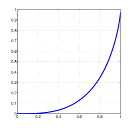
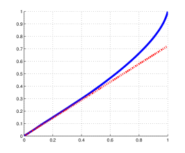
Figure 4: Figures show $N^{-1}\|b_{I}\|^{2}$ and $N_{I}^{-1/2}\|b_{I}\|$ vs. $N_{I}/N$. The red dotted line is $\sqrt{\pi/6}(N_{I}/N)$ vs. $N_{I}/N$.

Remark 2.8.

The following simulation illustrates that $x_{min}$ is a good initialization $x^{0}$. Use the alternating minimization of $x$ and $s$ to solve the problem

$$\min_{s}\min_{x}\|Ax-sb\|^{2},\;|s|=1.$$

Choose $A$ to be a Gaussian random matrix from $\mathbf{R}^{240\times 60}$ and $N_{I}=90$. Rescale both $x_{0},x^{*}$ to unit vectors, where $x^{*}$ is the vector $x$ at the final iteration. In Fig. 5, the reconstruction error is measured in terms of

$$\|x_{0}x_{0}^{\top}-x^{*}{x^{*}}^{\top}\|.$$

The figures in Fig. 5 show the results of $100$ trials using two different initializations. Obviously the singular vector is a good initialization.

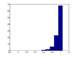
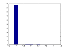
Figure 5: Figures show the histogram of the reconstruction error via the random initialization (left) and via the $x_{min}$ initialization (right).

2.4 ADM with rank-$r$

Under some circumstances, the singular vector corresponding to the least singular value becomes a poor initialization for $x_{0}$, for instance, in the presence of noise. Empirically, we find that the ADM with rank $r$ can alleviate the situation; see 3.2.

We propose the rank-$r$ method:

$$\min_{x\in\mathbf{R}^{n,r}}\frac{1}{2}\||Ax|-b\|^{2},$$ (2.10)

where $|z|$ refers to the vector whose $i$-th entry is the vector norm of the $i$-th row of the matrix $z$, i.e., $(\sum_{j=1}^{r}z_{i,j}^{2})^{1/2}$. Note that when $r=n$, the set $\{xx^{\top}:|Ax|=b\}$ is convex. In practical applications, we consider $r<n$ to save the computational load. Hence, instead of vectors $x,z$ in Eq. (2.1), we consider matrices $x\in\mathbf{R}^{n,r}$ and $z\in\mathbf{R}^{p,r}$ with $Ax=z$ in the non-convex minimization problem,

$$\min_{z,x}L(z,x,\lambda),$$ (2.11)

$$L(z,x,\lambda):=\{\frac{1}{2}\||z|-b\|^{2}+tr(\lambda^{\top}(Ax-z))+\frac{\beta}{2}\|Ax-z\|_{F}^{2}\}.$$ (2.12)

Similar to Alg. 2.1, we can adopt the ADM consisting of $z,x,\lambda$-iterations to solve the non-convex minimization problem. With $\lambda$ fixed, the optimal matrices $z,x$ have the following explicit expression.

Proposition 2.9.

Suppose $(z,x)$ is a minimizer in Eq. (2.11); then, $(zV,xV)$ is also a minimizer for any orthogonal matrix $V\in\mathbf{R}^{n,n}$. Moreover,

• for each $z$ fixed, $x=A^{\dagger}(z-\beta^{-1}\lambda)$ is the optimal matrix.

• Fixing $x$, write $u=Ax+\beta^{-1}\lambda$, then the optimality of $z$ is

  $$z=\frac{u}{|u|}\frac{b+\beta|u|}{1+\beta}.$$

Proof.

We only prove the $z$-part. The $x$-part is obvious. Because $L$ is separable in each row $z_{i}$ of $z$, then the optimization of $z_{i}$ can be solved via

$$\min_{z_{i}}\frac{1}{2}(\|z_{i}\|^{2}-2b_{i}\|z_{i}\|+b_{i}^{2})+\frac{\beta}{2}(\|u_{i}\|^{2}-2u_{i}\cdot z_{i}+\|z_{i}\|^{2}).$$

The optimality of $z_{i}$ occurs if and only if $z_{i}$ parallels $u_{i}/\|u_{i}\|$. Let $z_{i}=\alpha_{i}u_{i}/\|u_{i}\|$ with $\alpha_{i}$ to be determined. Thus,

$$\min_{\alpha_{i}}\frac{1}{2}(\alpha_{i}^{2}-2b_{i}|\alpha_{i}|+b_{i}^{2})+\frac{\beta}{2}(\|u_{i}\|^{2}-2\alpha_{i}\|u_{i}\|+\alpha_{i}^{2}).$$

Then, $\alpha_{i}\geq 0$ and

$$\alpha_{i}-b_{i}+\beta(\alpha_{i}-\|u_{i}\|)=0,$$

i.e., $\alpha_{i}=(1+\beta)^{-1}(b_{i}+\beta\|u_{i}\|)$ completes the proof. ∎

Empirical experimentation shows that the above ADM can usually yield an optimal solution $x\in\mathbf{R}^{n,r}$ with rank not equal to one, which does satisfy $|Ax|=b$. To recover the rank-one matrix $x_{0}x_{0}^{\top}$, we take the following steps. First, we standardize $A$ to be a matrix consisting of orthogonal columns via QR or SVD factorizations, such that $I_{n\times n}$ lies in the range of $\mathcal{A}$. Indeed,

$$\sum_{i=1}^{N}a_{i}a_{i}^{\top}=A^{\top}A=I_{n\times n}.$$

When $y\in\mathbf{R}^{n,r}$, we have $b^{2}\cdot e=tr(yy^{\top})=\|y\|^{2}_{F}$. Hence, the norm $\|y\|^{2}_{F}=\sum_{i=1}^{n}\sigma_{i}(y)^{2}$ remains constant for all the feasible solutions $\{y:|Qy|=b\}$, where $\sigma_{i}(y)$ refers to the singular values of $y$. Second, consider the objective function to retrieve the matrix $y$ with the maximal leading singular value,

$$\min_{y}\left(\frac{1}{2}\|Qy-z\|_{F}^{2}-\gamma\sigma_{1}(y)\right),$$ (2.13)

where $\gamma>0$ is some parameter to balance the fidelity $|Qy|=|z|=b$ and the maximization of the leading singular value $\sigma_{1}(y)$. Since the leading singular value of $y$ is maximized, there is no guarantee that we can always obtain the global optimal solution.

Proposition 2.10.

Write $Q^{\top}z$ in the SVD factorization,

$$Q^{\top}z=U_{z}D_{z}V_{z}^{\top}.$$

Then the optimal matrix $y$ in Eq. (2.13) is $y=U_{z}D_{y}V_{z}^{\top}$ in the SVD factorization, where $D_{y}=D_{z}+\gamma e_{1}e_{1}^{\top}$.

Proof.

Observe that

$$\frac{1}{2}\|Qy-z\|_{F}^{2}-\gamma\sigma_{1}(y)=\frac{1}{2}\|U_{z}^{\top}QU_{y}D_{y}V_{y}^{\top}V_{z}-D_{z}\|_{F}^{2}-\gamma D_{y}(1,1),$$

where $D_{y}(1,1)$ refers to the (1,1) entry of the diagonal matrix $D_{y}$. Due to the rotational invariance of the Frobenius norm, then the first term achieves its minimum when

$$U_{z}^{\top}QU_{y}D_{y}V_{y}^{\top}V_{z}=D_{z}+\alpha e_{1}e_{1}^{\top}$$ (2.14)

and $\alpha$ is the minimizer of

$$\min_{\alpha}\left(\alpha^{2}/2-\gamma(D_{z}(1,1)+\alpha)\right),\;i.e.,\alpha=\gamma.$$

Also, Eq. (2.14) yields $U_{z}^{\top}QU_{y}=I$ and $V_{y}^{\top}V_{z}=I$, which completes the proof. ∎

Remark 2.11.

Suppose that $|Ax|=b$ for some $x\in\mathbf{R}^{n,r}$. Then, the minimizer of

$$\min_{x}\left(\frac{1}{2}\||Ax|-b\|^{2}-\gamma\sigma_{1}(x)\right)$$

is $(1+\gamma)x_{0}$. Indeed, consider $x=\alpha x_{0}$. Then,

$$\alpha=arg\min_{\alpha}\left(\frac{1}{2}(\alpha-1)^{2}\|b\|^{2}-\gamma\alpha\right)=1+\gamma.$$

In Eq. (2.11), replacing $A$ with $Q$ and replacing the term $\frac{\beta}{2}\|Ax-z\|_{F}^{2}$ with

$$\beta\left(\frac{1}{2}\|Qy-z\|_{F}^{2}-\gamma\sigma_{1}(y)\right),$$

then we adopt the ADM to retrieve a rank-one solution.

Algorithm 2.12.

1. Initialize a random matrix $y\in\mathbf{R}^{n,r}$ and $\lambda^{0}=0_{N,r}\in\mathbf{R}^{N,r}$. Repeat the following steps, $k=1,2,\ldots$. Then let the solution $x^{*}$ be the first column of $U_{z}$, i.e., the singular vector corresponding to the maximal singular value.

2. $z$-iteration:

   $$u=Qy^{k}+\lambda^{k}\beta^{-1},\;z^{k+1}=\frac{u}{|u|}\frac{b+\beta|u|}{1+\beta},$$

3. $\lambda$-iteration:

   $$\lambda^{k+1}=\lambda^{k}+\beta(Qy^{k}-z^{k+1}),$$

4. $y$-iteration:

   $$U_{z}D_{z}V_{z}=Q^{\top}(z^{k+1}-\lambda^{k+1}\beta^{-1}),\;y^{k+1}=U_{z}(D_{z}+\gamma e_{1}).$$

2.5 Standardized frames with equal norm

In the simulations (section 3.1), we will show the importance of the unit norm condition $\|a_{i}\|=1$ for $i=1,\ldots,N$ in the ADM approach. When the QR factorization is used to generate an equivalent standardized matrix consisting of rows $\{a_{i}\}_{i=1}^{N}$, the sensing vectors $\{a_{i}\}$ do not have equal norm in general.

The following theorem states that we can standardize $A$ to obtain an orthogonal matrix $Q$ whose rows have equal norm. The proof is given in the appendix.

Theorem 2.13.

Given a matrix $A\in\mathbf{R}^{N\times n}$ satisfying the rank* condition and $N>n$, we can find a unique diagonal matrix $D$ with $D_{i,i}>0$, such that

$$D^{-1/2}A=QB,$$

and $Q$ is one standardized matrix, which is one projection matrix with $Q^{\top}Q=I_{n\times n}$, $(QQ^{\top})_{i,i}=(n/N)$ for all $i$, where $B$ is some $n\times n$ nonsingular matrix.

Here the diagonal value $n/N$ is the average of the norm $\|Q\|_{F}^{2}=tr(Q^{\top}Q)=tr(QQ^{\top})=n$. Also,

$$N=\|D^{1/2}A\|_{F}^{2}=\|QB\|_{F}^{2}=\|B\|_{F}^{2}.$$

With the uniqueness of $D$, $Q$ is also determined uniquely up to the right multiplication of an orthogonal matrix. Indeed, $B$ is uniquely determined up to the left multiplication of an orthogonal matrix:

$$A^{\top}D^{-1/2}D^{-1/2}A=B^{\top}Q^{\top}QB=B^{\top}B.$$

Recall that $A$ satisfies the rank* condition if any square $n$-by-$n$ sub-matrix of $A$ is full rank. When a matrix $A$ satisfies the rank* condition then there exists no orthogonal matrix $V\in\mathbf{R}^{n\times n}$, such that

$$AV=C=\left(\begin{array}[]{cc}C_{1,1}&0\\ 0&C_{2,2}\end{array}\right),$$ (2.15)

where the $0$s refer to zero sub-matrices with size $(N-N_{1})\times n_{1}$ and size $N_{1}\times(n-n_{1})$ and $C_{1,1}$ is an $N_{1}\times n_{1}$ matrix. Furthermore, the condition ensures that the norm of each row must be positive. It is easy to see that, with probability one, Gaussian random matrices satisfy the rank* condition.

3 Experiments

3.1 ADM failure experiments

Due to the nature of nonconvex minimization, the algorithm can fail to converge, which is indeed observed in the following two simulations.

First, let us denote the input data by $(A,b)$ with $b_{i}\neq 0$ and the unknown signal by $x_{0}$. Mathematically, solving problem (i)

$$|Ax_{0}|=b$$

is equivalent to solving problem (ii)

$$b_{i}^{-1}|a_{i}\cdot x_{0}|=1.$$

However, solving these two problems via the ADM [22] can yield different results.

Let $A$ be a real Gaussian random matrix, $A\in\mathbf{R}^{N\times n}$. Let $b=|Ax_{0}|$. Rescale the system by $b^{-1}$, i.e., the input data becomes $(b^{-1}A,1_{N\times 1})$, thus equal measurement values. Figure 6 shows the error $\||AA^{\dagger}z|-b\|$ at each iteration. Here we use the random initialization for $x^{0}$.

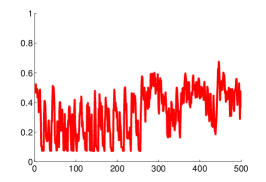
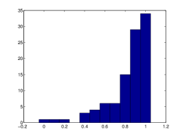
Figure 6: The left figure shows the error $\||AA^{\dagger}z|-b\|$ vs. the number of iteration via ADM with rank one [22]. The right figure shows the histogram $\|x_{0}x_{0}^{\top}-x^{*}{x^{*}}^{\top}\|$ of $100$ reruns.

Second, we demonstrate a few experiments where the ADM also fails to converge. The convergence failure sheds light on the importance of the two proposed assumptions in Section 2.2.

We sort a set of random generated sensing vectors $\{a_{i}\in\mathbf{R}^{100}\}_{i=1}^{400}$, such that

$$|a_{i}\cdot x_{0}|\leq|a_{j}\cdot x_{0}| i<j$$ for all .

That is, the indices are sorted according to the values $b_{i}$. We consider three different manners of selecting $200$ sensing vectors $\{a_{i}\}$: (1) the vectors with the smallest indices,(2) the vectors with the largest indices, and (3) a combination with $199$ small indices and one large index. Finally, we compare these results with the result using a random selection of sensing vectors, as shown in Fig. 7. Here, we fix rank $r=1$ and $\beta=0.01$. Clearly, the combination with smaller indices and larger indices performs best.

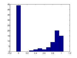
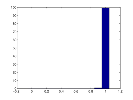
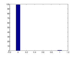
Figure 7: Figure shows the histogram $\|x_{0}x_{0}^{\top}-x^{*}{x^{*}}^{\top}\|$ under four different sets of $\{a_{i}\}_{i=1}^{400}$. In the top row, Left, middle and right subfigures show the results with $\{a_{i}\}_{i=1}^{200}$, with $\{a_{i}\}_{i=1}^{199}\cup\{a_{400}\}$ and with $\{a_{i}\}_{i=201}^{400}$. The bottom subfigure shows the result when randomly sampling $200$ sensing vectors.

3.2 Comparison experiments with noises

In this subsection, we demonstrate the performance of the ADM with $r=1$ and $r>1$ on a number of simulations, where Gaussian white noise is added. The noise-corrupted data, $b$, is generated,

$$b^{2}=\max((Ax_{0})^{2}+noise,0).$$

The signal-to-noise ratio is defined by

$$SNR=10\log_{10}\frac{\|Ax_{0}\|^{2}}{\|noise\|_{F}}.$$

In Fig. 8, we consider $A$ to be a real Gaussian random matrix with $N=2n$. We rerun the experiments $200$ times to test the effect of random initialization. The first row shows the histogram result with $n=30$ and $noise=0$. All the algorithms with $r=1,2,$ and $3$ work well. The second row shows the histogram result with $n=30$ and $SNR=29$. Here, we use $\beta=0.001$. Obviously the algorithms with $r>1$ have better performances.

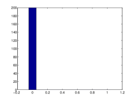
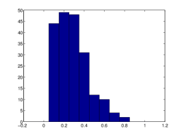
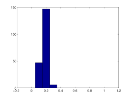
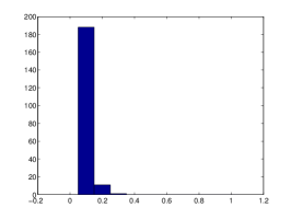
Figure 8: Figure shows the histogram $\|x_{0}x_{0}^{\top}-x^{*}{x^{*}}^{\top}\|$ under the noise effect. Left, middle and right columns show the results with rank $r=1$, $r=2$ and $r=3$. Here we use the random initialization.

Let $n=30$, $N=3n$ with $\beta=0.01$. In Fig. 9, we demonstrate the comparison between the random initialization and the singular vector initialization, i.e., the initialization is chosen to be the singular vector corresponding to the least singular value of $A_{I}\in\mathbf{R}^{45\times 30}$. Data $b$ is generated with $noise=2\times 10^{-4}\times Normal(0,1)$, $SNR=25dB$. Furthermore, with the presence of noise, when ADM with $r=1$ is employed, the difference between the two initializations is very little, in contrast to the simulation result shown in Remark 2.8.

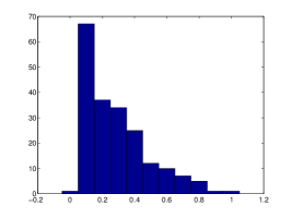
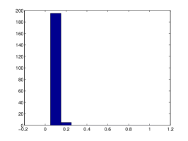
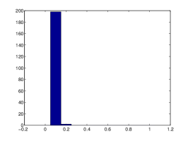
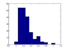
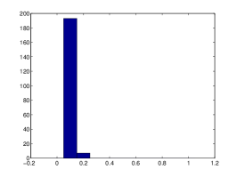
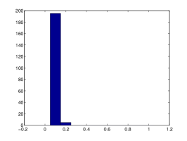
Figure 9: Figure shows the histogram $\|x_{0}x_{0}^{\top}-x^{*}{x^{*}}^{\top}\|$ of 200 trials under the noise effect. Left, middle and right columns show the results with rank $r=1$, $r=2$ and $r=3$. Here, we use the proposed initialization in the top row and the random initialization in the second row.

3.3 Phase retrieval experiments

Next, we report phase retrieval simulation results (Fourier matrices), with $x_{0}$ being real, positive images. Images are reconstructed subject to the positivity constraints ( i.e., the leading singular vector). The results are provided to show some advantage of ADM with $r=2$ over ADM with $r=1$. Here we use $\beta=0.1$ in the following experiment.

According to our experience, the phase retrieval with the Fourier matrix is a very difficult problem, in particular in the presence of noise. To alleviate the difficulty, researchers have suggested random illumination to enforce the uniqueness of solutions [9]. It is known that the phase retrieval has a unique solution up to three classes: constant global phase, spatial shift, and conjugate inversion. With high probability absolute uniqueness holds with a random phase illumination; see Cor. 1 [9].Our experiences show that the random phase illumination works much better than the above uniform illumination.

In Fig. 10, we demonstrate the the ADM with $r=1,2$ on the images with random phase illumination. Let $x_{0}\in\mathbf{R}^{300\times 300}$ be the intensity of the Lena image, see the bottom subfigure. We add noise and generate the data

$$b^{2}=\max(|Ax_{0}|^{2}+noise,0),$$

where $A$ is the Fourier matrix. The SNR is $39.8dB$ and the oversampling is $1.23$. Reconstruction errors $\|\frac{x^{*}}{\|x^{*}\|_{F}}-\frac{x_{0}}{\|x^{*}_{0}\|_{F}}\|_{F}$ for rank one and rank two are $0.126$ and $0.109$, respectively. The ADM with $r=2$ has a better reconstruction.

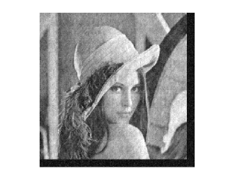
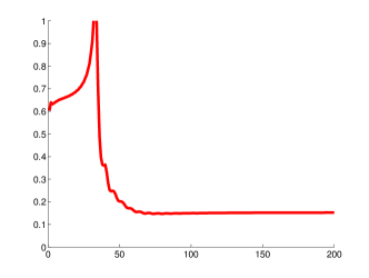
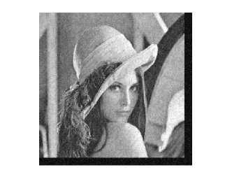
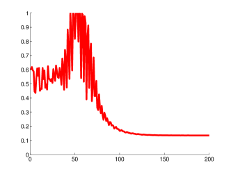
Figure 10: Figures show the reconstructed images and the error $\||AA^{\dagger}z|-b\|_{F}$ vs. the number of iteration via ADM with rank $r=1$ (the first row) and $r=2$ (the second row).

3.4 Conclusions

In this paper, we discuss the rank-one matrix recovery via two approaches. First, the rank-one matrix is computed among the Hermitian matrices as in PhaseLift. We make the observation that matrices in the feasible set have equal trace norm via the measurement matrices with orthonormal columns. Experiments show that with the aid of these orthogonal frames, exact recovery occurs under a smaller $N/n$ ratio compared with the PhaseLift in both real and complex cases. In the second part of the paper, we discuss the “lifting” of the nonconvex alternating direction minimization method from rank-one to rank-$r$ matrices, $r>1$. The benefit of this relaxation cannot be overestimated, because the construction of large Hermitian matrices is avoided, as is the associated Hermitian matrices projection. Comparing with the ADM with rank-one, the ADM with rank $r>1$ performs better in recovering noise-contaminated signals, which is demonstrated in simulation experiments.

Another contribution is the error estimate between the unknown signal and the singular vector corresponding to the least singular value. The initialization has an effect of importance in the nonconvex minimization. We demonstrate that a good initialization can be the least singular vector of the subset of sensing vectors corresponding to the small measurement values $b_{i}$. In the case of real Gaussian matrices, the error can be reduced, as the number of measurements grows at a rate proportional to the dimension of unknown signals. One of our future works is the generalization of the error estimate to complex frames, in particular the case of the Fourier matrix.

Appendix A Standardization of $A$

In the following, we will prove Theorem 2.13 in several steps. We discuss the existence first. The uniqueness analysis will be shown later. Fixing $A$, let $\mathcal{D}$ be the inverse matrices of diagonal matrices $D$,

$$\mathcal{D}:=\{D^{-1}\in\mathbf{R}^{N\times N}:\|D^{-1/2}A\|_{F}^{2}=\sum_{i=1}^{N}D_{i,i}^{-1}\sum_{j=1}^{n}A_{i,j}^{2}=N,D_{i.i}\geq 0\}.$$

Clearly $\mathcal{D}$ is nonempty and convex compact. In fact, $D_{i,i}$ has a positive lower bound,

$$D_{i,i}\geq N^{-1}\sum_{j=1}^{n}A_{i,j}^{2}\textrm{ for all $i$.}$$

For each $D^{-1}\in\mathcal{D}$, let $f:\mathcal{D}\to\mathcal{D}$ be the function

$$f(D^{-1})=\hat{D}^{-1},\textrm{ where $QB=D^{-1/2}A$ is the QR factorization},$$

and each row of $\hat{D}^{-1/2}AB^{-1}$ has norm one. In fact, the function $f$ generates iterations $\{(D^{k})^{-1}\}_{k=0}^{\infty}$ with $(D^{k+1})^{-1}=f((D^{k})^{-1})$. That is, start with $Q^{0}=A$. Repeat the two steps for $k=0,1,2,\ldots$ until it converges:

$$(ii) Q^{k} (D^{k})^{-1/2}Q^{k}$$ Normalize the row of by ;

$$(ii) \textrm{Take the QR factorization:}(D^{k})^{-1/2}Q^{k-1}=Q^{k}R^{k}.$$

Since $D^{-1/2}A$ has rank $n$, then $B$ has rank $n$ and $B^{-1}$ exists. The function $f$ is well defined: Once $B$ is given, then choose the diagonal matrix $D$ to be that which normalizes the rows of $AB^{-1}$. According to Brouwer’s fixed-point theorem, we have the existence of $D$, such that $D^{-1/2}AB^{-1}=Q$ consists of orthogonal columns and each row has norm one.

Before the uniqueness proof, we state one equation of $D$.

Proposition A.1.

The diagonal matrix $D$ satisfies the equation,

$$(n/N)D_{i,i}=(A(A^{\top}D^{-1}A)^{-1}A^{\top})_{i,i}.$$ (A.1)

Proof.

According to $D^{-1/2}A=QB$, we have

$$(n/N)D_{i,i}=(D^{1/2}QQ^{\top}D^{1/2})_{i,i}=(A(B^{\top}B)^{-1}A^{\top})_{i,i}.$$

Note that $B^{\top}B=A^{\top}D^{-1/2}Q^{\top}QD^{-1/2}A=A^{\top}D^{-1}A$. Thus,

$$\;(n/N)D_{i,i}=(A(A^{\top}D^{-1}A)^{-1}A^{\top})_{i,i}.$$

∎

Proposition A.2.

Let $p_{i}\in(0,1)$, $i=1,\ldots,n$ with $\sum_{i=1}^{n}p_{i}=1$. Let $\lambda_{i}>0$ for $i=1,\ldots,n$. Then

$$\sum_{i=1}^{n}p_{i}\lambda_{i}\geq(\sum_{i=1}^{n}p_{i}\lambda_{i}^{-1})^{-1},$$

where equality holds if and only if $\{p_{i}\}_{i=1}^{n}$ are equal.

Proof.

Let $f(x)=x^{-1}$ for $x>0$, which is strictly convex. The statement is the application of Jensen inequality,

$$\sum_{i=1}^{n}p_{i}\lambda_{i}^{-1}\geq(\sum_{i=1}^{n}p_{i}\lambda_{i})^{-1}.$$

∎

Proposition A.3.

Suppose that $Q$ is a standardized matrix satisfying the rank* condition. Let $F^{1}$ be a positive diagonal matrix. Then the iteration

$$F^{k+1}_{i,i}=(N/n)(Q(Q^{\top}(F^{k})^{-1}Q)^{-1}Q^{\top})_{i,i},\;k=1,\ldots.$$

yields $\lim_{k\to\infty}F^{k}=cI_{N\times N}$, where $c$ is some scalar.

Proof.

We will show $tr(F^{k+1})\leq tr(F^{k})$. Suppose that $\{(\lambda_{i}^{-1},q_{i})\}_{i}$ are eigenvalues-eigenvectors of $Q^{\top}(F^{k})^{-1}Q$, then $\{(\lambda_{i},q_{i})\}_{i}$ are eigenvalues-eigenvectors of $(Q^{\top}(F^{k})^{-1}Q)^{-1}$. Hence,

$$\lambda_{i}^{-1}=q_{i}^{\top}Q^{\top}(F^{k})^{-1}Qq_{i},$$

and

$$tr(F^{k+1})=\sum_{j=1}^{N}\mu^{k+1}_{j}=(N/n)\sum_{i=1}^{n}\lambda_{i}=(N/n)\sum_{i=1}^{n}(\sum_{j=1}^{N}(F^{k}_{j,j})^{-1}(Qq_{i})_{j}^{2})^{-1}.$$

Denote the j-th entry of $|(Qq_{i})_{j}|$ by $p_{j,i}$. Then $\sum_{j=1}^{N}p_{j,i}^{2}=1$ and $\sum_{i=1}^{n}p_{j,i}^{2}=n/N$. Let $\{\mu_{i}^{k}\}_{i=1}^{N}$ be the diagonal entries of $F^{k}$. Then

$$\sum_{j=1}^{N}\mu_{j}^{k+1}=(N/n)\sum_{i=1}^{n}(\sum_{j=1}^{N}(\mu^{k}_{j})^{-1}p_{j,i}^{2})^{-1}\leq(N/n)\sum_{i=1}^{n}\sum_{j=1}^{N}\mu^{k}_{j}p_{j,i}^{2}=\sum_{j=1}^{N}\mu^{k}_{j},$$

where the last equality is due to $\sum_{i=1}^{n}p_{j,i}^{2}=n/N$. Hence, $tr(F^{k+1})\leq tr(F^{k})$. Denote one of limiting points of $\mu^{k}_{i}$ by $\mu^{*}_{i}$ and then

$$(\sum_{j=1}^{N}p_{j,i}^{2}(\mu^{*}_{j})^{-1})^{-1}=\sum_{j=1}^{N}p_{j,i}^{2}\mu^{*}_{j}\textrm{ for all }i.$$

Hence, $\mu^{*}_{i}=\mu^{*}_{j}$ for all $i,j$ with $p_{j,i}>0$. Due to the rank* condition, $QV$ cannot be written in the form of Eq. (2.15) for any orthogonal matrix $V$ whose columns are orthonormal vectors $\{q_{i}\}_{i=1}^{n}$ with $p_{j,i}=|(QV)_{j,i}|$. Hence, $c=\mu^{*}_{i}=\mu^{*}_{j}$ for all $i,j$.

∎

Finally, we complete the proof in the following.

Proposition A.4.

Suppose that $A$ satisfies the rank* condition. Let $D_{*}$ be one solution of Eq. (A.1). Then with any positive diagonal matrix $D^{0}$, the iteration

$$D^{k+1}=(N/n)diag(A(A^{\top}(D^{k})^{-1}A)^{-1}A^{\top}),\;k=1,\ldots,$$

yields

$$\lim_{k\to\infty}D^{k}=D_{*}.$$

Thus, $D_{*}$ is unique.

Proof.

Let $D_{*}^{-1/2}A=QB$ be the QR factorization of $D_{*}^{-1/2}A$. Then

$$(A^{\top}D^{-1}A)^{-1}=B^{-1}(Q^{\top}(D_{*}^{-1/2}DD_{*}^{-1/2})^{-1}Q)^{-1}B^{-1},$$

and the iteration becomes

$$D^{-1/2}_{*}D^{k+1}D^{-1/2}_{*}=(N/n)diag(Q(Q^{\top}(D_{*}^{-1/2}D^{k}D_{*}^{-1/2})^{-1}Q)^{-1}Q^{\top}),\;k=1,\ldots.$$

Let $F^{k}=D^{-1/2}_{*}D^{k}D^{-1/2}_{*}$. Since $A$ satisfies the rank* condition, then for any nonsingular matrix $B$, $D_{*}^{-1/2}AB^{-1}$ also satisfies the rank* condition and cannot be written in the form in Eq. (2.15) for any orthogonal matrix. According to Prop. A.2, the proof is completed.

∎

References

- [1] Radu Balan, Pete Casazza, and Dan Edidin. On signal reconstruction without phase. Applied and Computational Harmonic Analysis, 20(3):345–356, 2006.
- [2] Afonso S. Bandeira, Jameson Cahill, Dustin G. Mixon, and Aaron A. Nelson. Saving phase: Injectivity and stability for phase retrieval. Applied and Computational Harmonic Analysis, 2013.
- [3] Heinz H. Bauschke, Patrick L. Combettes, and D. Russell Luke. Phase retrieval, error reduction algorithm, and Fienup variants: a view from convex optimization. J. Opt. Soc. Amer. A, 19:1334–1345, 2002.
- [4] E. Candès, Y. Eldar, T. Strohmer, and V. Voroninski. Phase retrieval via matrix completion. SIAM Journal on Imaging Sciences, 6(1):199–225, 2013.
- [5] Emmanuel J. Candès and Xiaodong Li. Solving quadratic equations via phaselift when there are about as many equations as unknowns. Foundations of Computational Mathematics, pages 1–10, 2013.
- [6] Emmanuel J. Candès, Thomas Strohmer, and Vladislav Voroninski. PhaseLift: Exact and stable signal recovery from magnitude measurements via convex programming. Communications on Pure and Applied Mathematics, 66(8):1241–1274, 2013.
- [7] Hung Chen. Lecture note. http://www.math.ntu.edu.tw/~hchen/teaching/LargeSample/notes/noteorder.pdf.
- [8] Laurent Demanet and Paul Hand. Stable optimizationless recovery from phaseless linear measurements. Journal of Fourier Analysis and Applications, pages 1–23, 2012.
- [9] Albert Fannjiang. Absolute uniqueness of phase retrieval with random illumination. Inverse Problems, 28(7):Article ID 075008, 20 p., 2012.
- [10] Albert Fannjiang and Wenjing Liao. Phase retrieval with random phase illumination. J. Opt. Soc. Am. A, 29(9):1847–1859, Sep 2012.
- [11] J. R. Fienup. Phase retrieval algorithms: a comparison. Appl. Opt., 21(15):2758–2769, Aug 1982.
- [12] R. W. Gerchberg and W. Owen Saxton. A practical algorithm for the determination of the phase from image and diffraction plane pictures. Optik, 35:237–246, 1972.
- [13] Guoyong Gu, Bingsheng He, and Xiaoming Yuan. Customized proximal point algorithms for linearly constrained convex minimization and saddle-point problems: a unified approach. Computational Optimization and Applications, pages 1–27, 2013.
- [14] N.E. Hurt. Phase Retrieval and Zero Crossings: Mathematical Methods in Image Reconstruction. Mathematics and Its Applications. Springer, 2001.
- [15] J. Miao, D. Sayre, and H. N. Chapman. Phase retrieval from the magnitude of the fourier transforms of nonperiodic objects. J. Opt. Soc. Am. A, 15(6):1662–1669, Jun 1998.
- [16] Jianwei Miao, Tetsuya Ishikawa, Qun Shen, and Thomas Earnest. Extending x-ray crystallography to allow the imaging of noncrystalline materials, cells, and single protein complexes. Annual Review of Physical Chemistry, 59(1):387–410, 2008. PMID: 18031219.
- [17] R. P. Millane. Phase retrieval in crystallography and optics. J. Opt. Soc. Am. A, 7(3):394–411, Mar 1990.
- [18] Mark Rudelson and Roman Vershynin. Non-asymptotic theory of random matrices: extreme singular values. Proceedings of the International Congress of Mathematicians, 2010.
- [19] Yoav Shechtman, Yonina C. Eldar, Oren Cohen, Henry N. Chapman, Jianwei Miao, and Mordechai Segev. Phase retrieval with application to optical imaging. CoRR, abs/1402.7350, 2014.
- [20] Roman Vershynin. Introduction to the non-asymptotic analysis of random matrices. CoRR, abs/1011.3027, 2010.
- [21] G.A. Watson. Characterization of the subdifferential of some matrix norms. Linear Algebra and its Applications, 170:33 – 45, 1992.
- [22] Zaiwen Wen, Chao Yang, Xin Liu, and Stefano Marchesini. Alternating direction methods for classical and ptychographic phase retrieval. Inverse Problems, 28(11):115010, 2012.