A Novel Approach to Finding Near-Cliques:
The Triangle-Densest Subgraph Problem

Abstract

Many graph mining applications rely on detecting subgraphs which are near-cliques. There exists a dichotomy between the results in the existing work related to this problem: on the one hand the densest subgraph problem (DS-Problem) which maximizes the average degree over all subgraphs is solvable in polynomial time but for many networks, fails to find subgraphs which are near-cliques. On the other hand, formulations that are geared towards finding near-cliques are $\mathbf{NP}$-hard and frequently inapproximable due to connections with the Maximum Clique problem.

In this work, we propose a formulation which combines the best of both worlds: it is solvable in polynomial time and finds near-cliques when the DS-Problem fails. Surprisingly, our formulation is a simple variation of the DS-Problem. Specifically, we define the triangle densest subgraph problem (TDS-Problem): given $G(V,E)$, find a subset of vertices $S^{*}$ such that $\tau(S^{*})=\max_{S\subseteq V}\frac{t(S)}{|S|}$, where $t(S)$ is the number of triangles induced by the set $S$. We provide various exact and approximation algorithms which the solve TDS-Problem efficiently. Furthermore, we show how our algorithms adapt to the more general problem of maximizing the $k$-clique average density. Finally, we provide empirical evidence that the TDS-Problem should be used whenever the output of DS-Problem fails to output a near-clique.

1 Introduction

A wide variety of graph mining applications relies on extracting dense subgraphs from large graphs. A list of some important such applications follows.

(1) Bader and Hogue observe that protein complexes, namely groups of proteins co-operating to achieve various biological functions, correspond to dense subgraphs in protein-protein interaction networks [BH03]. This observation is the cornerstone for several research projects which aim to identify such complexes, c.f. [BHG04, PLEO04, PWJ04].

(2) Sharan and Shamir notice that finding tight co-expression clusters in microarray data can be reduced to finding dense co-expression subgraphs [SS00]. Hu et al. capitalize on this observation to mine dense subgraphs across a family of networks [HYH⁺05].

(3) Fratkin et al. show an approach to finding regulatory motifs in DNA based on finding dense subgraphs [FNBB06].

(4) Iasemidis et al. rely on dense subgraph extraction to study epilepsy [IPSS01].

(5) Buehrer and Chellapilla show how to compress Web graphs using as their main primitive the detection of dense subgraphs [BC08].

(6) Gibson et al. observe that an algorithm which extracts dense subgraphs can be used to detect link spam in Web graphs [GKT05].

(7) Dense subgraphs are used for finding stories and events in micro-blogging streams [ASKS12].

(8) Alvarez-Hamelin et al. rely on dense subgraphs to provide a better understanding of the Internet topology [AHDBV06].

(9) In the financial domain, extracting dense subgraphs has been applied to, among others, predicting the behavior of financial instruments [BBP04], and finding price value motifs [DJD⁺09].

Among the various formulations for finding dense subgraphs, the densest subgraph problem (DS-Problem) stands out for the facts that is solvable in polynomial time [Gol84] and $\frac{1}{2}$-approximable in linear time [AHI02, Cha00, KS09]. To state the DS-Problem we introduce the necessary notation first. In this work we will focus on simple unweighted, undirected graphs. Given a graph $G=(V,E)$ and a subset of vertices $S\subseteq V$, let $G(S)=(S,E(S))$ be the subgraph induced by $S$, and let $e(S)=|E(S)|$ be the size of $E(S)$. Also, the edge density of the set $S$ is defined as $f_{e}(S)=e(S)/{|S|\choose 2}$. Notice that finding a subgraph which maximizes $f_{e}(S)$ is trivial. Since $0\leq f_{e}(S)\leq 1$ for any $S\subseteq V$, a single edge achieves the maximum possible edge density. Therefore, the direct maximization of $f_{e}$ is not a meaningful problem. The DS-Problem maximizes the ratio $\frac{e(S)}{|S|}$ over all subgraphs $S\subseteq V$. Notice that this is equivalent to maximizing the average degree. The DS-Problem is a powerful primitive for many graph applications including social piggybacking [GJL⁺13] reachability and distance query indexing [CHKZ02, JXRF09]. However, for many applications, including most of the listed applications, the goal is to find subgraphs which are near-cliques. Since the DS-Problem fails to find such subgraphs frequently by tending to favor large subgraphs with not very large edge density $f_{e}$ other formulations have been proposed, see Section 2. Unfortunately, these formulations are $\mathbf{NP}$-hard and also inapproximable due the connections with the Maximum Clique problem [Has99].

The goal of this work is to propose a tractable formulation which extracts near-cliques when the DS-Problem fails.

1.1 Contributions

The main contribution of this work is the following: we propose a novel objective which attacks efficiently the problem of extracting near-cliques from large graphs, an important problem for many applications, and is tractable. Specifically, our contributions are summarized as follows.

New objective. We introduce the average triangle density as a novel objective for finding dense subgraphs. We refer to the problem of maximizing the average triangle density as the triangle-densest subgraph problem (TDS-Problem).

Exact algorithms. We develop three exact algorithms for the TDS-Problem. The algorithm which achieves the best running time is based on maximum flow computations. It is worth outlining that Goldberg’s algorithm for the DS-Problem [Gol84] does not generalize to the TDS-Problem. For this purpose, we develop a novel approach that subsumes the DS-Problem and solves the TDS-Problem. Furthermore, our approach can solve a generalization of the DS-Problem and TDS-Problem that we introduce: maximize the average $k$-clique density for any $k$ constant.

Approximation algorithm. We propose a $\frac{1}{3}$-approximation algorithm for the TDS-Problem which runs asymptotically faster than any of the exact algorithms.

MapReduce implementation. We propose a $\frac{1}{3+3\epsilon}$-approximation algorithm for any $\epsilon>0$ which can be implemented efficiently in MapReduce. The algorithm requires $O(\log(n)/\epsilon)$ rounds and is MapReduce-efficient [KSV10] due to the existence of efficient MapReduce triangle counting algorithms [SV11].

Experimental evaluation. It is clear that in general the DS-Problem and the TDS-Problem can result in very different outputs. For instance, consider a graph which is the union of a triangle and a large complete bipartite clique. The DS-Problem problem is optimized via the bipartite clique, the TDS-Problem via the triangle. Based on experiments the two objectives behave differently on real-world networks as well. For all datasets we have experimented with, we observe that the TDS-Problem consistently succeeds in extracting near-cliques. For instance, in the Football network (see Table 1 for a description of the dataset) the DS-Problem returns the whole graph as the densest subgraph, with $f_{e}=0.094$ whereas the TDS-Problem returns a subgraph on 18 vertices with $f_{e}=0.48$.

Therefore, the TDS-Problem should be considered as an alternative to the DS-Problem when the latter fails to output near-cliques. Also, we perform numerous experiments on real datasets which show that the performance of the $\frac{1}{3}$-approximation algorithm is close to the optimal performance.

Graph mining application. We propose a modified version of the TDS-Problem, the constrained triangle densest subgraph problem (Constrainted-TDS-Problem), which aims to maximize the triangle density subject to the constraint that the output should contain a prespecified set of vertices $Q$. We show how to solve exactly the TDS-Problem. This variation is useful in various data-mining and bioinformatics tasks, see [TBG⁺13].

The paper is organized as follows: Section 2 presents related work. Section 3 defines and motivates the TDS-Problem. Section 4 presents our theoretical contributions. Section 5 presents experimental findings on real-world networks. Section 6 presents the Constrainted-TDS-Problem. Finally, Section 7 concludes the paper.

2 Related Work

In Sections 2.1 and 2.2 we review related work to finding dense subgraphs and counting triangles respectively.

2.1 Finding Dense Subgraphs

Clique. A clique is a set of vertices $S$ such that every two vertices in the subset are connected by an edge. The Clique problem, i.e., finding whether there is a clique of a given size in a graph is $\mathbf{NP}$-complete. A maximum clique of a graph $G$ is a clique of maximum possible size and its size is called the graph’s clique number. Finding the clique number is $\mathbf{NP}$-complete [Kar72]. Furthermore, H$\mathring{a}$stad proved [Has99] that unless P = NP there can be no polynomial time algorithm that approximates the maximum clique to within a factor better than $O(n^{1-\epsilon})$, for any $\epsilon>0$. When the max clique problem is parameterized by the order of the clique it is W[1]-hard [DF99]. Feige [Fei05] proposed a polynomial time algorithm that finds a clique of size $O\big{(}(\frac{\log{n}}{\log\log{n}})^{2}\big{)}$ whenever the graph has a clique of size $O(\frac{n}{\log{n}^{b}})$ for any constant $b$. This algorithm leads to an algorithm that approximates the max clique within a factor of $O\big{(}n\frac{(\log\log{n})^{2}}{\log{n}^{3}}\big{)}$. A maximal clique is a clique that is not a subset of a larger clique. A maximum clique is therefore always maximal, but the converse does not hold. The Bron-Kerbosch algorithm [BK73] is an exponential time method for finding all maximal cliques in a graph. A near optimal time algorithm for sparse graphs was introduced in [ELS10].

Densest Subgraph. In the densest subgraph problem we are given a graph $G$ and we wish to find the set $S\subseteq V$ which maximizes the average degree [Gol84, KV99]. The densest subgraph can be identified in polynomial time by solving a maximum flow problem [GGT89, Gol84]. Charikar [Cha00] proved that the greedy algorithm proposed by Asashiro et al. [AITT00] produces a $\frac{1}{2}$-approximation of the densest subgraph in linear time. Both algorithms are efficient in terms of running times and scale to large networks. In the case of directed graphs, the densest subgraph problem is solved in polynomial time as well [Cha00]. Khuller and Saha [KS09] provide a linear time $\frac{1}{2}$-approximation algorithm for the case of directed graphs among other contributions. We notice that there is no size restriction of the output, i.e., $|S|$ could be arbitrarily large. When restrictions on the size of $S$ are imposed the problem becomes $\mathbf{NP}$-hard. Specifically, the DkS problem, namely find the densest subgraph on $k$ vertices, is $\mathbf{NP}$-hard [AHI02]. For general $k$, Feige, Kortsarz and Peleg [FKP01] provide an approximation guarantee of $O(n^{\alpha})$ where $\alpha<1/3$. Currently, the best approximation guarantee is $O(n^{1/4+\epsilon})$ for any $\epsilon>0$ due to Bhaskara et al. [BCC⁺10]. The greedy algorithm of Asahiro et al. [AITT00] results in the approximation ratio $O(n/k)$. Therefore, when $k=\Omega(n)$ Asashiro et al. gave a constant factor approximation algorithm [AITT00]. It is worth mentioning that algorithms based on semidefinite programming have produced better approximation ratios for certain values of $k$ [FL01]. From the perspective of (in)approximability, Khot [Kho06] proved that that there does not exist any PTAS for the DkS problem under a reasonable complexity assumption. Arora, Karger, and Karpinski [AKK95] gave a PTAS for the special case $k=\Omega(n)$ and $m=\Theta(n^{2})$. Two interesting variations of the DkS problem were introduced by Andersen and Chellapilla [AC09]. The two problems ask for the set $S$ that maximizes the density subject to $s\leq k$ (DamkS) and $s\geq k$ (DalkS). They provide a practical 3-approximation algorithm for the DalkS problem and a slower 2-approximation algorithm. However it is not known whether DalkS is $\mathbf{NP}$-hard. For the DamkS problem they showed that if there exists a $\gamma$-approximation algorithm for DamkS, then there is a $4(\gamma^{2}+\gamma)$-approximation algorithm for the DkS problem, which indicates that DamkS is likely to be hard as well. This hardness conjecture was proved by Khuller and Saha [KS09].

Quasi-cliques. A set $S\subseteq V$ is a $\alpha$-quasiclique if $e(S)\geq\alpha{|S|\choose 2}$, i.e., if the edge density $f_{e}(S)$ exceeds a threshold parameter $0<\alpha\leq 1$. Abello et al. [ARS02] propose an algorithm for finding maximal quasi-cliques. Their algorithm starts with a random vertex and at every step it adds a new vertex to the current set $S$ as long as the density of the induced graph exceeds the prespecified threshold $\alpha$. Vertices that have many neighbors in $S$ and many other neighbors that can also extend $S$ are preferred. The algorithm iterates until it finds a maximal $\alpha$-quasi-clique. Uno presents an algorithm to enumerate all $\alpha$-pseudo-cliques [Uno10].

Recently, [TBG⁺13] introduced a general framework for dense subgraph extraction and proposed the optimal quasi-clique problem for extracting compact, dense subgraphs. The optimal quasi-clique problem is $\mathbf{NP}$-hard and inapproximable too [Tso13].

$k$-Core. A $k$-degenerate graph $G$ is a graph in which every subgraph has a vertex of degree at most k. The degeneracy of a graph is the smallest value of $k$ for which it is $k$-degenerate. The degeneracy is more known in the graph mining community as the $k$-core number. A $k$-core is a maximal connected subgraph of $G$ in which all vertices have degree at least $k$. There exists a linear time algorithm for finding $k$ cores by repeatedly removing the vertex of the smallest degree [BZ03]. A closely related concept is the triangle $k$-core, a maximal induced subgraph of $G$ for which each edge participates in at least $k$ triangles [ZP12]. To find a triangle $k$-core, edges that participate in fewer than $k$ triangles are repeatedly removed.

$k$-clubs, $kd$-cliques. A subgraph $G(S)$ induced by the vertex set $S$ is a $k$-club if the diameter of $G(S)$ is at most $k$ [Mok79]. $kd$-cliques are conceptually very close to $k$-clubs. The difference of a $kd$-clique from a $k$-club is that shortest paths between pairs of vertices from $S$ are allowed to include vertices from $V\backslash S$.

Shingling. Gibson, Kumar and Tomkins [GKT05] propose techniques to identify dense bipartite subgraphs via recursive shingling, a technique introduced by Broder et al. [BGMZ97]. This technique is geared towards large subgraphs and is based on min-wise independent permutations [BCFM98].

Triangle dense decompositions. Recently Gupta, Roughgarden and Seshadri prove constructively that when the graph has a constant transitivity ratio then the graph can be decomposed into disjoint dense clusters of radius at most two, containing a constant fraction of the triangles of $G$ [GRS14].

2.2 Triangle Counting

The state of the art algorithm for exact triangle counting is due to Alon, Yuster and Zwick [AYZ97] and runs in $O(m^{\frac{2\omega}{\omega+1}})$, where currently the fast matrix multiplication exponent $\omega$ is 2.3729 [Wil12]. Thus, their algorithm currently runs in $O(m^{1.4081})$ time. It is worth outlining that algorithms based on matrix multiplication are not practical even for medium sized networks due to the high memory requirements. For this reason, even if listing algorithms solve a more general problem than counting triangles, they are preferred for large graphs. Simple representative algorithms are the node- and the edge-iterator algorithms. In the former, the algorithm counts for each node the number of edges among its neighbors, whereas the latter counts for each edge $(i,j)$ the common neighbors of nodes’ $i,j$. Both have the same asymptotic complexity $O(mn)$, which in dense graphs results in $O(n^{3})$ time, the complexity of the naive counting algorithm. Practical improvements over this family of algorithms have been achieved using various techniques, such as hashing and sorting by the degree [Lat08, SW05]. The best known listing algorithm until recently was due to Itai and Rodeh [IR78] which runs in $O(m^{3/2})$ time. Recently, Björklund, Pagh, Williams and Zwick gave refined algorithms which are output sensitive algorithms [BPWVZ14]. Finally, it is worth mentioning that a large set of fast approximate triangle counting methods exist, e.g., [BYJK⁺02, BOV13, BFL⁺06, CJ14, JSP13, HTC13, NMPE12, PT12, PTTW13, SV11, TKMF09, TKM11].

3 Problem Definition

In this Section we define and motivate the main problem we consider in this work. We first define formally the notion of average triangle density.

Definition 1 (Triangle Density).

Let $G(V,E)$ be an undirected graph. For any $S\subseteq V$ we define its triangle density $\tau(S)$ as

$$\tau(S)=\frac{t(S)}{s},$$

where $t(S)$ is the number of triangles induced by $S$ and $s=|S|$.

Notice that $3\tau(S)$ is the average number of (induced) triangles per vertex in $S$. In this work we discuss the following problems which extend the well-known DS-Problem [Cha00, Gol84, KV99, KS09].

Problem 1 (TDS-Problem).

Given $G(V,E)$, find a subset of vertices $S^{*}$ such that $\tau(S^{*})=\tau^{*}_{G}$ where

$$\tau^{*}_{G}=\max_{S\subseteq V}\tau(S).$$

We will omit the index $G$ whenever it is obvious to which graph we refer to.

It is clear that the DS-Problem and TDS-Problem in general can result in significantly different solutions. Consider for instance a graph $G$ on $2n+3$ vertices which is the union of a triangle $K_{3}$ and of a bipartite clique $K_{n,n}$. The optimal solutions of the DS-Problem and the TDS-Problem are the bipartite clique and the triangle respectively. Therefore, the interesting question is whether maximizing the average degree and the triangle density result in different results in real-world networks.

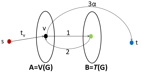
Figure 1: Figure shows the network $H$ that Algorithm 2 outputs, given a graph $G$ and a parameter $\alpha>0$ as its input. Set $A$ corresponds to the vertex set $V(G)$, whereas each vertex in set $B$ corresponds to a triangle in set $\mathcal{T}(G)$, the set of all triangles in $G$.

It is a well-known fact that triangles play a key role in numerous applications related to community detection and clustering, e.g., [GS, WS98]. This is reflected to the outcome of the TDS-Problem. Specifically, we observe that solving the TDS-Problem problem results in sets with a structure close to a clique. This is an important results for applications: as we have mentioned earlier, there exists a dichotomy among the various formulations used to extract dense subgraphs. Either the resulting optimization problem is $\mathbf{NP}$-hard or it is polynomially time solvable but tends to output subgraphs of larger size than the desired, which fail to be near-cliques.

As we will see in Section 5 in detail, the TDS-Problem consistently succeeds in finding near-cliques, even in cases where the DS-Problem fails. Furthermore, even when the DS-Problem succeeds in finding dense, compact subgraphs, the TDS-Problem output is always superior in terms of the edge density $f_{e}=e(S)/{|S|\choose 2}$ and triangle density $f_{t}=t(S)/{|S|\choose 3}$.

Table 2 shows the results of the optimal subgraphs for the DS-Problem and TDS-Problem respectively on some popular real-world networks. The results are representative on what we have observed on numerous datasets we have experimented with: the TDS-Problem optimal solution compared to the DS-Problem optimal solution is a smaller and tighter/denser subgraph which exhibits a strong near-clique structure. Therefore, the TDS-Problem appears to combine the best of both worlds: polynomial time solvability and extraction of near-cliques. On the other hand, since all algorithms we propose for the TDS-Problem require running first either a triangle listing or counting algorithm, we suggest that the TDS-Problem should be used in place of the DS-Problem, when the latter fails to extract a near-clique, as the former is computationally more expensive.

4 Proposed Method

Section 4.1 provides three algorithms which solve TDS-Problem exactly. Sections 4.2 and 4.3 provide a $\frac{1}{3}$-approximation algorithm for the TDS-Problem and an efficient MapReduce implementation respectively. Finally, Section 4.4 provides a generalization of the DS-Problem and the TDS-Problem to maximizing the average $k$-clique density and shows how the results from previous Sections adapt to this problem.

4.1 Exact Solutions

The algorithm presented in Section 4.1.1 achieves currently the best running time. We present an algorithm which relies on the supermodularity property of our objective in Section 4.1.2. It is worth outlining that even if the algorithm in Section 4.1.2 is slower, it requires less space than the algorithm in Section 4.1.1. Section 4.1.3 presents a linear programming approach which generalizes Charikar’s linear program [Cha00] to the TDS-Problem. Future improvements in the running time of procedures we use as black boxes, will imply improvements for our algorithms as well.

4.1.1 An $O\big{(}m^{3/2}+nt+\min{(n,t)}^{3}\big{)}$-time exact solution

1:  $l\leftarrow 0,u\leftarrow n^{3},S^{*}\leftarrow\emptyset$

2:  List the set of triangles $\mathcal{T}(G)$

3:  while $u\geq l+\frac{1}{n(n-1)}$ do

4:      $\alpha\leftarrow\frac{l+u}{2}$

5:      $H_{\alpha}\leftarrow$ Construct-Network$(G,\alpha,\mathcal{T}(G))$

6:     $(S,T)\leftarrow$ min $st$-cut in $H_{\alpha}$

7:     if $S=\{s\}$  then

8:        $u\leftarrow\alpha$

9:     else

10:        $l\leftarrow\alpha$

11:        $S^{*}\leftarrow\big{(}S\backslash\{s\}\big{)}\cap V(G)$

12:     end if

13:     Return $S^{*}$

14:  end while

Algorithm 1 triangle-densest subgraph$(G)$

1:  $V(H)\leftarrow\{s\}\cup V(G)\cup\mathcal{T}(G)\cup\{t\}$.

2:  For each vertex $v\in V(G)$ add an arc of capacity 1 to each triangle $t_{i}$ it participates in.

3:  For each triangle $\Delta=(u,v,w)\in\mathcal{T}(G)$ add arcs to $u,v,w$ of capacity 2.

4:  Add directed arc $(s,v)\in A(H)$ of capacity $t_{v}$ for each $v\in V(G)$.

5:  Add weighted directed arc $(v,t)\in A(H)$ of capacity $3\alpha$ for each $v\in V(G)$.

6:  Return network $H(V(H),A(H),w),s,t\in V(H)$.

Algorithm 2 Construct-Network $(G,\alpha,\mathcal{T}(G))$

Our main theoretical result is the following theorem. Its proof is constructive.

Theorem 1.

There exists a polynomial time algorithm which runs in $O\big{(}m^{3/2}+nt+\min{(n,t)}^{3}\big{)}$ time, where $n,t$ are the number of vertices and triangles in graph $G$ respectively, which solves the TDS-Problem in polynomial time.

We outline that the first term $O(m^{3/2})$ comes from using the Itai-Rodeh [IR78] as our triangle listing blackbox. If for instance we use the naive $O(n^{3})$ triangle listing algorithm then the running time expression is simplified to $O(n^{3}+nt)$. On the other hand, if we use the algorithms of Björklund et al. [BPWVZ14] the first term becomes for dense graphs $\tilde{O}\big{(}n^{\omega}+n^{3(\omega-1)/(5-\omega)}t^{2(3-\omega)/(5-\omega)}\big{)}$ and for sparse graphs $\tilde{O}\big{(}m^{2\omega/(\omega+1)}+m^{3(\omega-1)/(\omega+1)}t^{(3-\omega)/(\omega+1)}\big{)}$, where $\omega$ is the matrix multiplication exponent. Currently $\omega<2.3729$ due to [Wil12]. We maintain [IR78] as our black-box to keep the expressions simpler. However, the reader should keep in mind that the result presented in [BPWVZ14] improves the total running time of the first term.

We will work our way to proving Theorem 1 by proving first the following key lemma. Then, we will remove the logarithmic factor.

Lemma 1.

Algorithm 1 solves the TDS-Problem in $O\big{(}m^{3/2}+(nt+\min{(n,t)}^{3})\log(n)\big{)}$ time.

Algorithm 1 uses maximum flow computations to solve TDS-Problem. It is worth outlining that Goldberg’s maximum flow method [Gol84] for the DS-Problem does not adapt to the case of TDS-Problem. Algorithm 1 returns an optimal subgraph $S^{*}$, i.e., $\tau(S^{*})=\tau^{*}_{G}$. The algorithm performs a binary search on the triangle density value $\alpha$. Specifically, each binary search query corresponds to querying does there exist a set $S\subseteq V$ such that $t(S)/|S|>\alpha$?. For each binary search, we construct a network $H$ by invoking Algorithm 2. Let $\mathcal{T}(G)$ be the set of triangles in $G$. Figure 1 illustrates this network. The vertex set of $H$ is $V(H)=\{s\}\cup A\cup B\cup\{t\}$, where $A=V(G)$ and $B=\mathcal{T}(G)$. For the purpose of finding $\mathcal{T}(G)$, a triangle listing algorithm is required [BPWVZ14, IR78]. The arc set of graph $H$ is created as follows. For each vertex $r\in B$ corresponding to triangle $\Delta(u,v,w)$ we add three incoming and three outcoming arcs. The incoming arcs come from the vertices $u,v,w\in A$ which form triangle $\Delta(u,v,w)$. Each of these arcs has capacity equal to 1. The outgoing arcs go to the same set of vertices $u,v,w$, but the capacities are equal to 2. In addition to the arcs of capacity 1 from each vertex $u\in A$ to the triangles it participates in, we add an outgoing arc of capacity $3\alpha$ to the sink vertex $t$. From the source vertex $s$ we add an outgoing arc to each $u\in A$ of capacity $t_{v}$, where $t_{v}$ is the number of triangles vertex $v$ participates in $G$. As we have already noticed, $H$ can be constructed in $O(m^{3/2})$ time [IR78]. It is worth outlining that after computing $H$ for the first time, subsequent networks need to update only the arcs that depend on the parameter $\alpha$, something not shown in the pseudocode for simplicity. To prove that Algorithm 1 solves the TDS-Problem and runs in $O\big{(}m^{3/2}+(nt+\min{(n,t)}^{3})\log(n)\big{)}$ time we will proceed in steps.

For the sake of the proof, we introduce the following notation. For a given set of vertices $S$ let $t_{i}(S)$ be the number of triangles that involve exactly $i$ vertices from $S$, $i\in\{1,2,3\}$. Notice that $t_{3}(S)$ is the number of induced triangles by $S$, for which we have been using the simpler notation $t(S)$ so far.

We use the following claim as our criterion to set the initial values $l,u$ in the binary search.
Claim 1 $0\leq\tau(S)<n^{3}$ for any $S\subseteq V$.
The lower bound is trivial. The upper bound also follows trivially by observing that $t_{3}(S)\leq{n\choose 3}$ and $|S|\geq 1$ for any $\emptyset\neq S\subseteq V$. This suggests that the optimal value $\tau^{*}$ is always less than $n^{3}$.

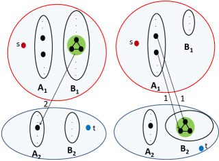
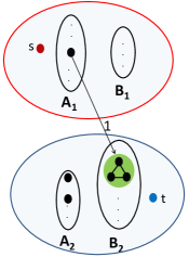
(a)	(b)	(c)

Figure 2: Figure shows the structure of any minimum $st$-cut $(S,T)$ in network $H_{\alpha}$, $\alpha>0$. Sets $S,T$ are shown within the ovals on the top (red) and the bottom (blue) respectively. Figure shows the structure with respect to three vertices $u,v,w\in A$ (in black) which form a triangle and the corresponding triangle-vertex $r\in B$ (green) for the case of a (a) type 3, (b) type 2 and (c) type 1 triangle.

The next claim serves as a criterion to decide when to stop the binary search.
Claim 2 The smallest possible difference among two distinct values $\tau(S_{1}),\tau(S_{2})$ is equal to $\frac{1}{n(n-1)}$.
To see why, notice that the difference $\delta$ between two possible different triangle density values is

$$\delta=\frac{t(S_{1})|S_{2}|-t(S_{2})|S_{1}|}{|S_{1}||S_{2}|}.$$

If $|S_{1}|=|S_{2}|$ then $|\delta|\geq\frac{1}{n}>\frac{1}{n(n-1)}$, otherwise $|\delta|\geq\frac{1}{|S_{1}||S_{2}|}\geq\frac{1}{n(n-1)}$. Notice that combining the above two claims shows that the binary search terminates in at most $5\log{n}$ queries. The following lemma is the key lemma for the correctness of Algorithm 1.

Lemma 2.

Consider any $st$ min-cut $(S,T)$ in network $H_{\alpha}$. Let $A_{1}=S\cap A,B_{1}=S\cap B$ and $A_{2}=T\cap A,B_{2}=T\cap B$. The cost of the min-cut is equal to

$$\sum_{v\notin A_{1}}t_{v}+2t_{2}(A_{1})+t_{1}(A_{1})+3\alpha|A_{1}|.$$

Proof.

Case I: $A_{1}=\emptyset$: In this case the proposition trivially holds, as the cost is equal to $\sum_{v\in A}t_{v}=3t$. It is worth noticing that in this case $B_{1}$ has to be also empty, otherwise we contradict the optimality of $(S,T)$. Hence $S=\{s\},T=A\cup B\cup\{t\}$.

Case II: $A_{1}\neq\emptyset$:

Consider the cost of the arcs from $A_{1}\cup B_{1}$ to $A_{2}\cup B_{2}$. We consider three different subcases, which are illustrated in Figure 2 If there exist three vertices $u,v,w\in A_{1}$ that form triangle $\Delta(u,v,w)$, then the vertex $r\in B$ corresponding to this specific triangle has to be in $B_{1}$. If not, then $r\in B_{2}$, and we could reduce the cost of the min-cut by 3, if we move the triangle to $B_{1}$. Therefore the cost we pay for triangles of type three is 0. This is shown in Figure 2(a). Consider three vertices $u,v,w$ such that they form a triangle $\Delta(u,v,w)$ and $u,v\in A_{1},w\in A_{2}$. Then, the vertex $r\in B$ corresponding to this triangle can be either in $B_{1}$ or $B_{2}$. The crucial point is that we always pay 2 in the cut for each triangle of type two as Figure 2(b) shows. Finally, in the case $u,v,w$ form a triangle, $u\in A_{1},v,w\in A_{2}$ the vertex $r\in B$ corresponding to triangle $\Delta(u,v,w)$ will be in $B_{2}$. If not, then it lies in $B_{1}$ and we could decrease the cost of the cut by 3 if we move it in $B_{2}$. Hence, we pay 1 in the cut for each triangle of type one as Figure 2(c) shows. Therefore the total cost is equal to $2t_{2}(A_{1})+t_{1}(A_{1})$.

Furthermore, the cost of the arcs from source $s$ to $T$ is equal to $\sum_{v\in A_{2}}t_{v}=\sum_{v\notin A_{1}}t_{v}$. The cost of the arcs from $A_{1}$ to $T$ is equal to $3\alpha|A_{1}|$. Summing up the individual cost terms, we obtain that the cost is equal to $\sum_{v\notin A_{1}}t_{v}+2t_{2}(A_{1})+t_{1}(A_{1})+3\alpha|A_{1}|$. ∎

The next lemma proves the correctness of the binary search in Algorithm 1.

Lemma 3.

(a) If there exists a set $W\subseteq V(G)$ in $G$ such that $t_{3}(W)>\alpha|W|$ then any $st$-min-cut (S,T) in $H_{\alpha}$ satisfies $S\backslash\{s\}\neq\emptyset$. (b) Furthermore, if there does not exists a set $W$ such that $t_{3}(W)>\alpha|W|$ then the cut $(\{s\},A\cup B\cup\{t\})$ is a minimum $st$-cut.

Proof.

(a) Let $W\subseteq V$ be such that

$$t_{3}(W)>\alpha|W|.$$ (1)

Suppose for the sake of contradiction that the minimum $st$-cut is achieved by $(\{s\},A\cup B\cup\{t\})$. In this case the cost of the minimum $st$-cut is $\sum_{v\in A}t_{v}=3t$. Now, consider the following $(S,T)$ cut. Set $S$ consists of the source vertex $s$, $A_{1}=W$ and $B_{1}$ be the set of triangles of type 3 and 2 induced by $A_{1}$. Let $T$ be the rest of the vertices in $H$. The cost of this cut is

$$cap(S,T)=\sum_{v\notin A_{1}}t_{v}+2t_{2}(A_{1})+t_{1}(A_{1})+3\alpha|A_{1}|.$$

Therefore, by our assumption that the minimum $st$-cut is achieved by $(\{s\},A\cup B\cup\{t\})$ we obtain

$$3t\leq\sum_{v\notin A_{1}}t_{v}+2t_{2}(A_{1})+t_{1}(A_{1})+3\alpha|A_{1}|.$$ (2)

Now, notice that by double counting

$$\sum_{v\in A_{1}}t_{v}=3t_{3}(A_{1})+2t_{2}(A_{1})+t_{1}(A_{1}).$$

Furthermore, we observe

$$\sum_{v\in A_{1}}t_{v}+\sum_{v\notin A_{1}}t_{v}=3t.$$

By combining these two facts, and the fact that $3t$ is the capacity of the minimum cut, we obtain the following contradiction of Inequality (1).

$$3t\leq\sum_{v\notin A_{1}}t_{v}+2t_{2}(A_{1})+t_{1}(A_{1})+3\alpha|A_{1}| \Leftrightarrow t_{3}(W)\leq\alpha|W|.$$

(b) By Lemma 2, for any minimum $st$-cut $(S,T)$ the capacity of the cut is equal to $\sum_{v\notin A_{1}}t_{v}+2t_{2}(A_{1})+t_{1}(A_{1})+3\alpha|A_{1}|$ where $A_{1}=A\cap S,A_{2}=A\cap T$. Suppose for the same of contradiction that the cut $(\{s\},A\cup B\cup\{t\})$ is not a minimum cut. Therefore,

$$cap(\{s\},A\cup B\cup\{t\})=3t>\sum_{v\notin A_{1}}t_{v}+2t_{2}(A_{1})+t_{1}(A_{1})+3\alpha|A_{1}|.$$

Using the same algebraic analysis as in (a), the above statement implies the contradiction $t_{3}(W)>\alpha|W|$, where $W=A_{1}$. ∎

Now we can complete the proof of Lemma 1.

Proof.

The termination of Algorithm 1 follows directly from Claims 1, 2. The correctness follows from Lemmata 2, 3. The running time follows from Claims 1,2 which show that the number of binary search queries is $O(\log(n))$ and each binary search query can be performed in $O\big{(}nt+\min{(n,t)}^{3}\big{)}$ time using the algorithm due to Ahuja, Orlin, Stein and Tarjan [AOST94] or Gusfield’s algorithm [Gus91]. ∎

The proof of Theorem 1 follows Lemma 1 and the fact that the parametric maximum flow algorithm of Ahuja, Orlin, Stein and Tarjan [AOST94], see also [GGT89], saves the logarithmic factor from the running time.

4.1.2 An $O\big{(}(n^{5}m^{1.4081}+n^{6}))\log(n)\big{)}$-time exact solution

In this Section we provide a second exact algorithm for the TDS-Problem. First, we provide the necessary theoretical background.

Definition 2 (Supermodular function).

Let $V$ be a finite set. The set function $f:2^{V}\rightarrow\mathbb{R}$ is supermodular if and only if for all $A,B\subseteq V$

$$f(A\cup B)\geq f(A)+f(B)-f(A\cap B).$$

A function $f$ is supermodular if and only if $-f$ is submodular.

Sub- and supermodular functions constitute an important class of functions with various exciting properties. In this work, we are primarily interested in the fact that maximizing a supermodular function is solvable in strongly polynomial time [GLS88, IFF01, Lov83, Sch00]. For our purposes, we state the following result which we use as a subroutine in our proposed algorithm.

Theorem 2 ([Orl09]).

There exists an algorithm for maximizing an integer valued supermodular function $f$ which runs in $O\big{(}n^{5}EO+n^{6})\big{)}$ time, where $n=|V|$ is the size of the ground set $V$ and $EO$ is the maximum amount of time to evaluate $f(S)$ for a subset $S\subseteq V$.

We show in the following that when the ground set is the set of vertices $V$ and $f_{\alpha}:2^{V}\rightarrow\mathbb{R}$ is defined by $f_{\alpha}(S)=t(S)-\alpha|S|$ where $\alpha\in\mathbb{R}^{+}$, we can solve the TDS-Problem in polynomial time.

Theorem 3.

Function $f:V\rightarrow\mathbb{R}$ where $f(S)=t(S)-\alpha|S|$ is supermodular.

Proof.

Let $A,B\subseteq V$. Let $t:2^{V}\rightarrow\mathbb{R}$ be the function which for each set of vertices $S$ returns the number of induced triangles $t(S)$. By careful counting

$$t(A\cup B)=t(A)+t(B)-t(A\cap B)+t_{1}(A:B\backslash A)+t_{2}(A:B\backslash A),$$

where $t_{1}(A:B\backslash A),t_{2}(A:B\backslash A)$ are the number of triangle with one, two vertices in $A$ and two, one vertices in $B\backslash A$ respectively. Hence, for any $A,B\subseteq V$

$$t(A\cup B)+t(A\cap B)\geq t(A)+t(B)$$

and the function $t$ is supermodular. Furthermore, for any $\alpha>0$ the function $-\alpha|S|$ is supermodular. Since the sum of two supermodular functions is supermodular, the result follows. ∎

Theorem 3 naturally suggests Algorithm 3. The algorithm will run in a logarithmic number of rounds. In each round we maximize function $f_{\alpha}$ using Orlin’s algorithm Orlin-Supermodular-Opt which takes as input arguments the graph $G$ and the parameter $\alpha>0$. We assume for simplicity that within the procedure Orlin-Supermodular-Opt function $f$ is evaluated using an efficient exact triangle counting algorithm [AYZ97]. The algorithm of Alon, Yuster and Zwick [AYZ97] runs in $O(m^{2\omega/(\omega+1)})$ time where $\omega<2.3729$ [Wil12]. This suggests the $EO=O(m^{1.4081})$. The overall running time of Algorithm 3 is $O\big{(}(n^{5}m^{1.4081}+n^{6})\log(n)\big{)}$.

1:  $l\leftarrow 0,u\leftarrow n^{3},S^{*}\leftarrow V$

2:  while $u\geq l+\frac{1}{n(n-1)}$ do

3:      $\alpha\leftarrow\frac{l+u}{2}$

4:      $(val,S)\leftarrow$ Orlin-Supermodular-Opt$(G,\alpha)$

5:     if $val<0$  then

6:        $u\leftarrow\alpha$

7:     else

8:        $l\leftarrow\alpha$

9:        $S^{*}\leftarrow S$

10:     end if

11:     Return $S^{*}$

12:  end while

Algorithm 3 triangle-densest subgraph$(G)$ [Supermodularity]

4.1.3 A Linear Programming Approach

In this Section we show how to generalize Charikar’s linear program, see $\S$2 in [Cha00], to provide a linear program (LP) which solves the TDS-Problem. The main difference compared to Charikar’s LP is the fact that we introduce a variable $x_{ijk}$ for each triangle $(i,j,k)\in\mathcal{T}(G)$. The LP follows.

$$\mathbf{max}\qquad\sum_{(i,j,k)\in\mathcal{T}(G)}x_{ijk} \mbox{{\bf s.t.} }\,\,x_{ijk}\leq y_{i} \forall(i,j,k)\in\mathcal{T}(G) \mbox{ }\,\,x_{ijk}\leq y_{j} \forall(i,j,k)\in\mathcal{T}(G) \mbox{ }\,\,x_{ijk}\leq y_{k} \forall(i,j,k)\in\mathcal{T}(G) \mbox{ }\,\,\sum_{i}y_{i}\leq 1 \mbox{ }\,\,x_{ijk}\geq 0 \forall(i,j,k)\in\mathcal{T}(G) \mbox{ }\,\,y_{i}\geq 0 \forall i\in V(G)$$

Theorem 4.

Let $OPT_{LP}$ be the value of the optimal solution to the LP 4.1.3. Then,

$$\tau_{G}^{*}=OPT_{LP}.$$

Furthermore, a set $S$ achieving triangle density equal to $\tau_{G}^{*}$ can be computed from the optimal solution to the LP.

Proof.

We break the proof of $\tau_{G}^{*}=OPT_{LP}$ in two cases. The second case provides a constructive procedure for finding a set $S^{*}$ which achieves triangle density equal to $\tau_{G}^{*}$.

Case I: $\tau_{G}^{*}\leq OPT_{LP}$
We will prove a more general statement: for any $S\subseteq V$, the value of the $LP$ is at least $\tau(S)$. We provide a feasible LP solution which achieves an objective value equal to $\tau(S)$. Let $y_{i}=\frac{1}{|S|}\mathbbm{1}(i\in S)$ for each $i\in V$. For each triangle $\Delta(i,j,k)$ induced by $S$ let $x_{ijk}=\frac{1}{|S|}$. For every other triangle $\Delta(i,j,k)$ set $x_{ijk}=0$. This is a feasible solution to the LP which achieves an objective value equal to $\frac{t(S)}{|S|}$. By setting $S=S^{*}$, we obtain $\tau_{G}^{*}\leq OPT_{LP}$.

Case II: $\tau_{G}^{*}\geq OPT_{LP}$
Let $(\bar{x},\bar{y})$ be the optimal solution to the LP. We define $S(r)=\{i:\bar{y}_{i}\geq r\}$, $T(r)=\{\Delta(i,j,k)\in\mathcal{T}(G):\bar{x}_{ijk}\geq r\}$. Notice that since $\bar{x}_{ijk}\leq\min{(\bar{y}_{i},\bar{y}_{j},\bar{y}_{k})}$, the inequality $\bar{x}_{ijk}\geq r$ implies that vertices $i,j,k$ belong in set $S(r)$. Furthermore, $\int_{0}^{1}|S(r)|dr=\sum_{i=1}^{n}\bar{y}_{i}\leq 1$ and $\int_{0}^{1}|T(r)|dr=\sum_{\Delta{(i,j,k)}}x_{ijk}$. If we assume that there exists no value $r$ such that $|T(r)|/|S(r)|\geq OPT_{LP}$ we obtain the contradiction

$$OPT_{LP}=\int_{0}^{1}|T(r)|dr<OPT_{LP}\int_{0}^{1}|S(r)|dr\leq OPT_{LP}.$$

Hence, $\tau_{G}^{*}\geq OPT_{LP}$. To find a set $S^{*}$ that achieves triangle density at least $OPT_{LP}$, we need to check at most $n$ different values of $r$ and checking the corresponding sets $S(r)$. ∎

4.2 A $\frac{1}{3}$-approximation algorithm

In this Section we provide an algorithm for the TDS-Problem which provides a $\frac{1}{3}$-approximation. Our algorithm follows the peeling paradigm, see [AITT00, Cha00, KS09, JMT13]. Specifically, in each round it removes the vertex which participates in the smallest number of triangles and returns the subgraph that achieves the largest triangle density. The pseudocode is shown in Algorithm 4.

1:  $n\leftarrow|V|,H_{n}\leftarrow G$

2:  for $i\leftarrow n$ to $2$ do

3:     Let $v$ be the vertex of $G_{i}$ of minimum number of triangles

4:     $G_{i-1}\leftarrow G_{i}\backslash{v}$

5:  end for

6:  Return $H_{j}$ that achieves maximum triangle density among $H_{i}$s, $i=1,\ldots,n$.

Algorithm 4 Peel-Triangles$(G)$

Theorem 5.

Algorithm 4 is a $\frac{1}{3}$-approximation algorithm for the TDS-Problem.

Proof.

Let $S^{*}$ be an optimal set. Let $v\in S^{*},|S^{*}|=s^{*}$ and $t_{A}(v)$ be the number of induced triangles by $A$ that $v$ participates in. Then,

$$\tau^{*}_{G}=\frac{t(S^{*})}{s^{*}}\geq\frac{t(S^{*}\backslash\{v\})}{s^{*}-1} \Leftrightarrow t_{S^{*}}(v)\geq\tau^{*}_{G},$$

since $t(S^{*}\backslash\{v\})=t(S^{*})-t_{S^{*}}(v)$. Consider the iteration before the algorithm removes the first vertex $v$ that belongs in $S^{*}$. Call the set of vertices $W$. Clearly, $S^{*}\subseteq W$ and for each vertex $u\in W$ the following lower bound holds $t_{W}(u)\geq t_{W}(v)\geq t_{S^{*}}(v)>\tau^{*}_{G}$ due to the greediness of Algorithm 3. This provides a lower bound on the total number of triangles induced by $W$

$$t(W) =\frac{1}{3}\sum_{u\in W}t_{W}(u)\geq\frac{1}{3}|W|\tau^{*}_{G}\Rightarrow\frac{t(W)}{|W|}\geq\frac{1}{3}\tau^{*}_{G}.$$

To complete the proof, notice that the algorithm returns a subgraph $S$ such that $\tau(S)\geq\tau(W)\geq\frac{1}{3}\tau^{*}_{G}$. ∎

In Section 5.1 we provide a simple implementation which runs in $O\big{(}\sum_{v}{deg(v)\choose 2}\big{)}=O(mn)$ time with the use of extra space. The key differences compared to the DS-Problem peeling algorithm [Cha00], are (i) we need to count triangles initially and (b) when we remove a vertex, the counts of its neighbors can decrease more than 1 in general. Therefore, when vertex $v$ is removed, we update the counts of its neighbors in $O\Big{(}{deg(v)\choose 2}\Big{)}$ time.

4.3 MapReduce Implementation

The MapReduce framework [DG08] has become the de facto standard for processing large-scale datasets. Since the original work of Dean and Ghemawat [DG08], a lot of research has focused on developing efficient algorithms for various graph theoretic problems including the densest subgraph problem [BKV12], minimum spanning trees [KSV10, LMSV11], finding connected components [KTF09, KSV10, LMSV11] and estimating the diameter [KTA⁺11], triangle counting [PT12, SV11, TKM11] and matchings, covers and min-cuts [LMSV11].

In the following, we show how we can approximate efficiently the TDS-Problem in MapReduce. Before we describe the algorithm, we show that Algorithm 5 for any $\epsilon>0$ terminates and provides a $\frac{1}{3+3\epsilon}$-approximation. The idea behind this algorithm is to peel vertices in batches [BKV12, GP11] rather than one by one.

1:   $S_{out},S\leftarrow V$

2:  while  $S\neq\emptyset$ do

3:      $A(S)\leftarrow\{i\in S:t_{S}(i)\leq 3(1+\epsilon)\tau(S)\}$

4:      $S\leftarrow S\backslash A(S)$

5:     if $\tau(S)\geq\tau(S_{out})$ then

6:         $S_{out}\leftarrow S$

7:     end if

8:  end while

9:  Return $S_{out}$.

Algorithm 5 Peel-Triangles-in-Batches$(G,\epsilon>0)$

Lemma 4.

For any $\epsilon>0$, Algorithm 5 provides a $\frac{1}{(3+3\epsilon)}$-approximation to the TDS-Problem. Furthermore, it terminates in $O(\log_{1+\epsilon}(n))$ passes.

Proof.

Let $S^{*}$ be an optimal solution to the TDS-Problem. As we proved in Theorem 5, for any $v\in S^{*}$ it is true that $t_{S^{*}}(v)\geq\tau^{*}_{G}$. Furthermore, in each round at least one vertex is removed. To see why, assume for the sake of contradiction that $A(S)=\emptyset$ for some $S$ during the execution of the algorithm. Then, we obtain the contradiction that $3|S|\tau(S)=\sum_{v\in S}t_{S}(v)\geq(3+3\epsilon)|S|\tau(S)$. Consider the round where the algorithm for the first time removes a vertex $v\in S^{*}$. Let $W$ be the corresponding set of vertices. Since $v\in A(W)$ is peeled off, we obtain an upper bound on its induced degree, namely $v\in A(W)\Rightarrow t_{W}(v)\leq(3+3\epsilon)\tau(W)$. Since $S^{*}\subseteq W$, we obtain

$$(3+3\epsilon)\tau(W) \geq t_{W}(v)\geq t_{S^{*}}(v)\geq\tau(S^{*}),$$

which proves that Algorithm 5 is a $\frac{1}{(3+3\epsilon)}$-approximation to the TDS-Problem. To see why the algorithm terminates in logarithmic number of rounds, notice that

$$3t(S) >\sum_{v\in S\backslash A(S)}t_{S}(v)\geq(3+3\epsilon)\big{(}|S|-|A(S)|\big{)}\frac{t(S)}{|S|}\Leftrightarrow$$

$$|A(S)| \geq\frac{\epsilon}{1+\epsilon}|S|\Leftrightarrow|S\backslash A(S)|\leq\frac{1}{1+\epsilon}|S|.$$

Since $S$ decreases by a factor of $\frac{1}{1+\epsilon}$ in each round, the algorithm terminates in $O(\log_{1+\epsilon}(n))=O\big{(}\frac{\log(n)}{\epsilon}\big{)}$ rounds.

MapReduce Implementation: Now we are able to describe our algorithm in MapReduce. It uses any of the efficient algorithms of Suri and Vassilvitski [SV11] as a subroutine to count triangles per vertex in each round. The removal of the vertices which participate in less triangles than the threshold, is done in two rounds, as in [BKV12]. For completeness, we describe the procedure here. The set of vertices $S$ to be peeled off in each round are marked by adding a key-value pair $\langle v;\$\rangle$ for each $v\in S$. Each edge $(u,v)$ is mapped to $\langle u;v\rangle$. The reducer receives all endpoints of the edges incident with $v$ and the symbol $\$$ in case the vertex is marked for deletion. In case the vertex is marked, then the reduce task returns nothing, otherwise it copies its input. In the second round, we perform the same procedure with the only difference being that we map each edge $(u,v)$ to $\langle v;u\rangle$. Therefore, the edges which remain have both endpoints unmarked. The algorithm runs in $O(\log(n)/\epsilon)$, as it takes $O(\log(n)/\epsilon)$ peeling off rounds, and in each peeling round, constant number of rounds is needed to count triangles per vertex, mark vertices for deletion and remove the corresponding vertex set.

4.4 $k$-clique Densest Subgraph

We outline that our proposed methods can be adapted to the following generalization of DS-Problem and TDS-Problem.

Definition 3 ($k$-clique-densest subgraph).

Let $G(V,E)$ be an undirected graph. For any $S\subseteq V$ we define its $k$-clique density $h_{k}(S)$, $k\geq 2$ as

$$h_{k}(S)=\frac{c_{k}(S)}{s},$$

where $c_{k}(S)$ is the number of $k$-cliques induced by $S$ and $s=|S|$.

Problem 2 (k-Clique-DS-Problem).

Given $G(V,E)$, find a subset of vertices $S^{*}$ such that $h_{k}(S^{*})=h^{*}_{k}$ where

$$h^{*}_{k}=\max_{S\subseteq V}h_{k}(S).$$

As in the triangle densest subgraph problem, we create a network $H$ parameterized by the value $\alpha$ on which we perform our binary search. The procedure is described in Algorithm 6. The set $\mathcal{C}(G)$ is the set of $k$-cliques in $G$. We then invoke Algorithm 1, with the upper bound $u$ set to $n^{k}$. Following the analysis of Theorem 1, we see that the k-Clique-DS-Problem is solvable in polynomial time. For instance, using Gusfield’s algorithm [Gus91] or [AOST94] in each binary search query we get an overall running time $O\big{(}n^{k}+(n|\mathcal{C}(G)|+n^{3})\log(n)\big{)}=O(n^{k+1}\log(n))$. Using the improved result due to Ahuja, Orlin, Stein and Tarjan for parametric max flows in unbalanced bipartite graphs [AOST94], we save the logarithmic factor in the running time.

1:  $V(H)\leftarrow\{s\}\cup V(G)\cup\mathcal{C}(G)\cup\{t\}$.

2:  For each vertex $v\in V(G)$ add an arc of capacity 1 to each $k$-clique $c_{i}$ it participates in.

3:  For each $k$-clique $(u_{i_{1}},\ldots,u_{i_{k}})\in\mathcal{C}(G)$ add arcs to $u_{i_{1}},\ldots,u_{i_{k}}$ of capacity $k-1$.

4:  Add directed arc $(s,v)\in A(H)$ of capacity $c_{v}$ for each $v\in V(G)$.

5:  Add weighted directed arc $(v,t)\in A(H)$ of capacity $k\alpha$ for each $v\in V(G)$.

6:  Return network $H(V(H),A(H),w),s,t\in V(H)$.

Algorithm 6 Construct-Network-$k$ $(G,\alpha,\mathcal{C}(G),k)$

Furthermore, Algorithm 4 can also be modified, by removing in each round the vertex with the smallest number of $k$-cliques, to obtain Corollary 2. As the analogy of Theorem 5.

Corollary 1.

The algorithm which peels off in each round the vertex with the minimum number of $k$-cliques and returns the subgraph that achieves the largest $k$-clique density, is a $\frac{1}{k}$-approximation algorithm for the k-Clique-DS-Problem.

Similarly, Algoritm 5 and the MapReduce implementation can be modified to solve the k-Clique-DS-Problem. We omit the details.

Corollary 2.

The algorithm which peels off in each round the set of vertices with less than $k(1+\epsilon)h(S)$, where $h(S)$ is the $k$-clique density in that round, terminates in $O(\log_{1+\epsilon}(n))$ rounds and provides a $\frac{1}{k(1+\epsilon)}$-approximation guarantee for the k-Clique-DS-Problem. Furthermore, using [FFF14], we obtain an efficient MapReduce implementation.

We notice that in general there exist benefits from moving to higher order $k$ values. Consider the following example which can be further formalized (details omitted). Let $G\sim G(n,p)$ be an Erdös-Rényi graph, where $p=p(n)$. Assume that we plant a clique $K$ of size $n^{\gamma}$ for some constant $\gamma>0$. We wish to show a non-trivial range of $p=p(n)$ values such that the following conditions hold:

$$h_{2}(C)=\frac{|E(K)|}{|K|}=\frac{{n^{\gamma}\choose 2}}{n^{\gamma}}<\frac{p{n\choose 2}}{n}={\mathbb{E}}\left[{h_{2}(V)}\right]$$

.

and for $k\geq 3$

$$h_{k}(C)=\frac{{n^{\gamma}\choose k}}{n^{\gamma}}>\frac{p^{{k\choose 2}}{n\choose k}}{n}={\mathbb{E}}\left[{h_{k}(V)}\right]$$

By simple algebraic manipulation we see that $p$ satisfies both conditions if

$$O\big{(}n^{-(1-\gamma)}\big{)}<p<O\big{(}n^{-\tfrac{2}{k}(1-\gamma)}\big{)}.$$

Clearly, for larger $k$ values, we allow ourselves a larger range of $p$ values for which we can find the hidden clique in expectation. We have implemented the algorithms for k-Clique-DS-Problem but we defer the experimental analysis on real graphs for an extended version of this work. Our main finding from preliminary results with $k=4$, is that in few cases there exists a benefit to maximizing the average $K_{4}$ density. However, the gain obtained by moving from the DS-Problem to the TDS-Problem with respect to extracting a near-clique is larger than the gain by moving the TDS-Problem to the $4$-clique-densest subgraph.

Name	Nodes	Edges	Description
Adjnoun	112	425	Generated by processing text data
AS-735	6 475	12 572	Autonomous Systems
AS-caida	26 475	53 381	Autonomous Systems
ca-Astro	17 903	196 972	Person to Person
ca-GrQC	4 158	13 422	Person to Person
Celegans	297	4 296	Neural network of C. Elegans
DBLP	53 442	255 936	Person to Person
Epinions	75 877	405 739	Person to Person
Enron	33 696	180 811	Email
EuAll	224 832	339 925	Email
Football	115	613	NCAA football game network
Karate	34	78	Person to Person
Lesmis	77	254	Generated by processing text data
Political blogs	1 490	16 715	Generated by processing sales data
Political books	105	441	Blog network
soc-Slashdot0811	77 360	469 180	Person to Person
soc-Slashdot0902	82 168	504 230	Person to Person
wb-cs-Stanford	8 929	26 320	Web Graph (page to page)

Table 1: Datasets used in our experiments.

5 Experimental Evaluation

Method	Measure	Adjnoun	Celegans	Football	Karate	Lesmis	Polblogs	Polbooks
	$\frac{|S|}{|V|}$(%)	42.86	45.8	100	47.1	29.9	19.1	51.4
	$\delta$	9.58	17.16	10.66	5.25	10.78	55.82	9.40
DS	$f_{e}$	0.20	0.13	0.094	0.35	0.49	0.196	0.18
	$\tau$	14	45.93	21.12	5.64	41.61	768.87	22.68
	$f_{t}$	0.013	0.005	0.003	0.05	0.18	0.019	0.016
	$\frac{|S|}{|V|}$(%)	41.1	42.4	100	52.9	29.9	18.7	57.1
	$\delta$	9.57	17.1	10.66	5.2	10.78	55.8	9.3
$\frac{1}{2}$-DS	$f_{e}$	0.21	0.14	0.094	0.31	0.49	0.20	0.16
	$\tau$	14.16	46.5	21.12	5.16	41.61	774.6	22.68
	$f_{t}$	0.014	0.006	0.003	0.04	0.18	0.02	0.013
	$\frac{|S|}{|V|}$(%)	36.6	10.4	15.7	17.7	16.9	8.1	19.1
	$\delta$	9.37	13.81	8.22	4.67	10.62	55.72	9.34
TDS	$f_{e}$	0.23	0.46	0.48	0.93	0.89	0.46	0.50
	$\tau$	15	56.82	28	8.01	47.31	972.36	25.95
	$f_{t}$	0.019	0.13	0.21	0.80	0.72	0.136	0.15
	$\frac{|S|}{|V|}$(%)	36.6	9.1	15.7	17.7	16.9	8.1	15.2
	$\delta$	9.37	13.56	8.22	4.67	10.62	55.72	9.13
$\frac{1}{3}$-TDS	$f_{e}$	0.23	0.52	0.48	0.93	0.89	0.46	0.61
	$\tau$	15	56.55	28	8.01	47.31	972.36	25.5
	$f_{t}$	0.019	0.17	0.21	0.80	0.72	0.136	0.24

Table 2: Comparison of the extracted subgraphs by the Goldberg’s exact algorithm for the DS-Problem (DS), Charikar’s $\frac{1}{2}$-approximation algorithm ($\frac{1}{2}$-DS), our exact algorithm for the TDS-Problem (TDS) and our $\frac{1}{3}$-approximation algorithm ($\frac{1}{2}$-TDS). Here, $f_{e}(S)=e(S)/{|S|\choose 2}$ is the edge density of the extracted subgraph, $\delta(S)=2e(S)/|S|$ is the average degree, $f_{t}(S)=t(S)/{|S|\choose 3}$ is the triangle density and $\tau(S)=3t(S)/|S|$ is the average number of triangles per vertex.

The main goal of this Section is to show that the proposed algorithms for the TDS-Problem constitute new graph mining primitives that can be used to find near-cliques when the DS-Problem fails. Additionally to this goal, we compare the quality of the $\frac{1}{3}$-approximation algorithm (Algorithm 4) to the optimal algorithm. Finally, we explore the trade-off between the approximation quality and the number of rounds by ranging the parameter $\epsilon$ in Algorithm 5.

5.1 Experimental Setup

The datasets we use are shown in Table 1. The experiments were performed on a single machine, with Intel(R) Core(TM) i5 CPU at 2.40 GHz, with 3.86GB of main memory. We have implemented Algorithm 1 in Matlab R2011a using a maximum flow implementation due to Kolmogorov and Boykov [BK04] as our subroutine which runs in time $O(t(n+t)^{3})$. This implementation can be prohibitively expensive even for small graphs which have a large number of triangles. In the next section we evaluate the exact algorithm on a subset of graphs.

The space usage due to the construction of the network $H_{\alpha}$ -which has $O(n+t)$ vertices and $O(n+t)$ arcs- can be large as many networks have a large number of triangles. It is worth outlining that when the space usage is a problem whereas the running time is not, the supermodularity algorithm can be used instead. Furthermore, it is also worth mentioning that using any standard maximum flow algorithm rather than the algorithm of Ahuja et al. [AOST94] results in an expensive algorithm which runs in $\tilde{\Omega}((n+t)^{2})$ time.We have written an efficient implementation of our peeling algorithm in Java JDK 1.6 which runs in $O(nm)$ time. Our implementation maintains an array of size $O(n)$ containing the counts of triangles per vertex and an array of at most $O(\max_{v}t_{v})$ entries each one pointing to a hash table (notice there exist at most $n$ entries with non-empty hash tables). The hash table at position $i$ of the array keeps the set of vertices with exactly $i$ participating triangles. At any iteration, we maintain the minimum index of the array pointing to a non-empty hash table. When we remove a vertex, we update the triangle counts of its neighbors, move them and place them in the appropriate hash table if needed, and if one of the updated counts is less than the number of triangles that the index points at, then we update the index accordingly. The total running time is $O\Big{(}{deg(v)\choose 2}\Big{)}=O(nm)$. We measure the quality of each extracted subgraph by two measures: the edge density of the extracted subgraph $f_{e}=e(S)/{|S|\choose 2}$ and the triangle density $f_{t}=t(S)/{|S|\choose 3}$. Notice that when $f_{e},f_{t}$ are close to 1, the extracted subgraph is close to being a clique.

5.2 Experiments

Table 2 shows the results obtained on several popular small- and medium-sized graphs. Each column corresponds to a dataset. The rows correspond to measurements for each method we use to extract a subgraph. Specifically, the first (DS), second ($\tfrac{1}{2}$-DS), third (TDS) and fourth ($\tfrac{1}{3}$-TDS) row corresponds to the subgraph extracted by Goldberg’s exact algorithm [Gol84] for the DS-Problem, Charikar’s $\tfrac{1}{2}$-approximation algorithm [Cha00] for the DS-Problem, Algorithm 1 and Algorithm 4 for the TDS-Problem respectively. For each optimal extracted subgraph $S$, we show its size as a fraction of the total number of vertices, the edge density $f_{e}(S)$, the average degree $\delta(S)=2e(S)/|S|$, the triangle density $f_{t}(S)$ and the average number of triangles per vertex $\tau(S)=3t(S)/|S|$. We observe that for all datasets, the optimal triangle-densest subgraph is close to being a near-clique while the optimal densest subgraph is not always so. A pronounced example is the Football network where the optimal densest subgraph is the whole network with $f_{e}=0.0094$, whereas the optimal triangle-densest subgraph is a set of 18 vertices with edge density 0.48. Finally, we observe that the quality of Algorithm’s 4 output is very close to the optimal solution and sometimes even better. It is worth mentioning that the same phenomenon is observed in the case of Charikar’s $\frac{1}{2}$-approximation algorithm [Cha00] compared to Goldberg’s exact algorithm [Gol84].

We use the scalable Java implementation of Algorithm 4 and a scalable implementation of Charikar’s $\frac{1}{2}$-approximation algorithm on the rest of the datasets of Table 1. The results are shown in Table 3. Again, we verify the fact that the TDS-Problem results in near-cliques, even when the DS-Problem fails. For instance, for the collaboration network ca-Astro the DS-Problem results in a subgraph with 1 184 vertices with $f_{e}=0.05,f_{t}=0.002$. The TDS-Problem results in a clique with 57 vertices. The experimental results in Tables 2 and 3 strongly indicate that the algorithms developed in this work consitute graph mining primitives that can be used to extract near-cliques when the DS-Problem problem fails to do so.

	$\frac{1}{2}$-DS			$\frac{1}{3}$-TDS
	$|S|$	$f_{e}$	$f_{t}$	$|S|$	$f_{e}$	$f_{t}$
AS-735	59	0.28	0.08	13	0.8	0.66
AS-caida	143	0.14	0.02	27	0.52	0.25
ca-Astro	1 184	0.05	0.002	57	1	1
ca-GrQC	42	0.79	0.68	14	0.89	0.84
Epinions	718	0.27	0.10	135	0.60	0.33
Enron	192	0.30	0.07	139	0.40	0.12
EuAll	248	0.20	0.01	108	0.40	0.18
soc-Slashdot0811	1 637	0.29	0.08	253	0.52	0.29
soc-Slashdot0902	1 787	0.28	0.07	247	0.49	0.23
wb-cs-Stanford	84	0.64	0.48	26	0.80	0.67

Table 3: Comparison of the extracted subgraphs by the $\frac{1}{2}$-approximation algorithm of Charikar and the $\frac{1}{3}$-approximation algorithm, Algorithm 4.

5.3 Exploring parameter $\epsilon$ in Algorithm 5

In this Section we present the results of Algorithm 5 on the DBLP graph. This is particularly interesting instance as it indicates that instead of thinking for to select a good $\epsilon$ value, it is worth trying out at least few when resources are available. We range $\epsilon$ from 0.1 to 1.8 with a step of 0.1. Figure 3(a) plots the number of rounds Algorithm 5 takes to terminate as a function of $\epsilon$. We observe that even for small $\epsilon$ values the number of rounds is 6. The reader should compare this to the upper bound predicted by Lemma 4 which exceeds 100. Figure 3(b) plots the relative ratio $Rel.~{}\tau=\frac{\tau(S)}{\tau_{G}^{*}}$ where $S$ is the output of Algorithm 5. For convenience, the lower bound $\frac{1}{3+3\epsilon}$ is plotted with red color. Similarly, Figure 3(c) plots the relative ratios $\frac{f_{e}(S)}{f_{e}(S^{*})},\frac{f_{t}(S)}{f_{t}(S^{*})}$ as a function of $\epsilon$. As we observe, the quality of Algorithm 5 is close to the optimal solution except for $\epsilon=0.7$ and $\epsilon=0.8$. By inspecting why this happens we observe that the optimal triangle-densest subgraph is a clique of 44 vertices. It turns out that for $\epsilon=0.7,0.8$ the optimal subgraph which is found in the last round of the execution of the algorithm (the latter happens for all $\epsilon$ values) consists of 98 and 74 vertices which contain as a subgraph the optimal $K_{44}$. For other values of $\epsilon$, the subgraph in the last round is either the optimal $K_{44}$ or close to it, with few more extra vertices. This example shows the potential danger of using a single value for $\epsilon$, suggesting that trying out a small number of $\epsilon$ values can be significantly beneficial in terms of the approximation quality.

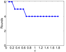
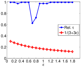
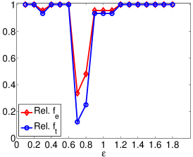
(a)	(b)	(c)

Figure 3: Exploring the trade-off between the number of rounds and accuracy as a function of the parameter $\epsilon$ for Algorithm 5. Let $S,S^{*}$ be the extracted subgraphs by Algorithms 5 and 1 respectively. (a) Number of rounds, (b) relative average triangle density ratio $\frac{\tau(S)}{\tau_{G}^{*}}$ (blue $*$) and the approximation guarantee $1/(3+3\epsilon)$ (red $\diamond$), and (c) relative ratios $\frac{f_{e}(S)}{f_{e}(S^{*})},\frac{f_{t}(S)}{f_{t}(S^{*})}$ as functions of $\epsilon$.

6 Application: Organizing Cocktail Parties

A graph mining problem that comes up in various applications is the following: given a set of vertices $Q\subseteq V$, find a dense subgraph containing $Q$ We refer to this type of graph mining problems as cocktail problems, due to the following motivation, c.f. [SG10]. Suppose that a set of people $Q$ wants to organize a cocktail party. How do they invite other people to the party so that the set of all the participants, including $Q$, are as similar as possible? A variation of the TDS-Problem which addresses this graph mining problem follows.

Problem 3 (Constrainted-TDS-Problem).

Given $G(V,E)$ and $Q\subseteq V$, find the subset of vertices $S^{*}$ that maximizes the triangle density such that $Q\subseteq S^{*}$ ,

$$S^{*}=\arg\max_{Q\subseteq S\subseteq V}\tau(S).$$

The Constrainted-TDS-Problem can be solved by modifying our proposed algorithms accordingly. A useful corollary follows.

Corollary 3.

The Constrainted-TDS-Problem is solvable in polynomial time by adding arcs from $s$ to $v\in A$ of large enough capacities, e.g., capacities equal to $n^{3}+1$ are sufficiently large. Furthermore, the peeling algorithm which avoids removing vertices from $Q$ is a $\frac{1}{3}$-approximation algorithm for the Constrainted-TDS-Problem.

In the following we evaluate the $\frac{1}{3}$-approximation algorithm on two datasets. The two experiments indicate two different types of performances that should be expected in real-world applications. The first is a positive whereas the second is negative case. Both experiments here serve as sanity checks

Political vote data. We obtain Senate data for the first session (2006) of the 109th congress which spanned the period from January 3, 2005 to January 3, 2007, during the fifth and sixth years of George W. Bush’s presidency [wik]. In this Congress, there were 55, 45 and 1 Republican, Democratic and independent senators respectively. The dataset can be downloaded from the US Senate web page http://www.senate.gov. We preprocess the dataset in the following way: we add an edge between two senators if amonge the bills for which they both casted a vote, they voted at least 80% of the times in the same way. The resulting graph has 100 vertices and 2034 edges. We run the $\frac{1}{3}$-approximation algorithm on this graph using as our set $Q$ the first three republicans according to lexicographic order: Alexander (R-TN), Allard (R-CO) and Allen (R-VA). We obtain at our output a subgraph consisting of 47 vertices. By inspecting their party, we find that 100% of them are Republicans. This shows that our algorithm in this case succeeds in finding the large majority of the cluster of republicans. It is interesting that the 8 remaining Republicans do not enter the triangle-densest subgraph. A careful inspection of the data, c.f. [pre], indicates that 6 republicans agree with the party vote on at most 79% of the bills, and 8 of them on at most 85% of the bills.

DBLP graph. We input as a query set $Q$ a set of scientists who have established themselves in theory and algorithm design: Richard Karp, Christos Papadimitriou, Mihalis Yannakakis and Santosh Vempala. The algorithm returns at its output the query set and a set $S$ of 44 vertices corresponding to a clique of (mostly) Italian computer scientists. We list a subset of the 44 vertices here: M. Bencivenni, M. Canaparo, F. Capannini, L. Carota, M. Carpene, R. Veraldi, P. Veronesi, M. Vistoli, R. Zappi. The output graph induced by $S\cup Q$ is disconnected. Therefore, this can be easily explained because of the following (folklore) inequality, given that $|Q|<|S|$ in our example.

Claim 1.

Let $a,b,c,d$ be non-negative. Then,

$$\max{\big{(}\frac{a}{c},\frac{b}{d}\big{)}}\geq\frac{a+b}{c+d}\geq\min{\big{(}\frac{a}{c},\frac{b}{d}\big{)}}$$ (4)

In our example, we get $a=t(S),c=|S|,b=t(Q),d=|Q|$. In such a scenario, where the output consists of the union of a dense subgraph and the query set $Q$, an algorithm which builds itself up from $Q$ -assuming $Q$ is not an independent set- to $V$ by adding vertices which create as many triangles as possible and returning the maximum density subgraph, rather than peeling vertices from $V$ downto $Q$ should be preferred in practice, see also [TBG⁺13].

7 Conclusion

In this work we introduce the average triangle density as a novel objective for attacking the important problem of finding near-cliques. We propose exact and approximation algorithms and an efficient MapReduce implementation. Furthermore, we show how to generalize our results to maximizing the average $k$-clique density. Experimentally we verify the value of the TDS-Problem as a novel addition to the graph mining toolbox. Also, we show how to solve a constrained version of the TDS-Problem which has various graph mining applications.

Our work leaves numerous problems open, including the following: (a) Can we obtain a better exact solution? (b) How do approximate triangle counting methods affect the outcome of the $\frac{1}{3}$-approximation algorithm? (c) Are there real-world networks where TDS-Problem fails to extract near-cliques? In those networks, can the k-Clique-DS-Problem problem for $k$ constant render the situation in an analogy of how the TDS-Problem succeeds in cases where the DS-Problem fails? We have implemented the exact algorithm in Section 4.4 and we have tested for $k=4$, namely maximizing the average $K4$ density. Preliminary results on various graph datasets suggest that there can be gains when one uses higher $k$-values but the gain obtained from moving from the DS-Problem to the TDS-Problem is typically significantly larger from the gain obtained (if any) from the TDS-Problem to larger $k$ values. (d) It is clear that one can extract the top-$k$ non-overlapping triangle densest subgraphs, using $k$ executions of one of our algorithms. For instance, extracting the top-7 triangle-densest subgraphs from the DBLP graph results in finding 7 cliques of size 44, 27, 25, 24, 20, 20 and 19 Can we compute such dense subgraphs simultaneously?

References

- [AC09] Reid Andersen and Kumar Chellapilla. Finding dense subgraphs with size bounds. In WAW, 2009.
- [AHDBV06] J Ignacio Alvarez-Hamelin, Luca Dall Asta, Alain Barrat, and Alessandro Vespignani. How the k-core decomposition helps in understanding the internet topology. In ISMA Workshop on the Internet Topology, 2006.
- [AHI02] Yuichi Asahiro, Refael Hassin, and Kazuo Iwama. Complexity of finding dense subgraphs. Discr. Ap. Math., 121(1-3), 2002.
- [AITT00] Yuichi Asahiro, Kazuo Iwama, Hisao Tamaki, and Takeshi Tokuyama. Greedily finding a dense subgraph. J. Algorithms, 34(2), 2000.
- [AKK95] Sanjeev Arora, David Karger, and Marek Karpinski. Polynomial time approximation schemes for dense instances of NP-hard problems. In STOC, 1995.
- [AOST94] Ravindra K Ahuja, James B Orlin, Clifford Stein, and Robert E Tarjan. Improved algorithms for bipartite network flow. SIAM Journal on Computing, 23(5):906–933, 1994.
- [ARS02] James Abello, Mauricio G. C. Resende, and Sandra Sudarsky. Massive quasi-clique detection. In LATIN, 2002.
- [ASKS12] A. Angel, N. Sarkas, N. Koudas, and D. Srivastava. Dense subgraph maintenance under streaming edge weight updates for real-time story identification. Proc. VLDB Endow., 5(6):574–585, February 2012.
- [AYZ97] Noga Alon, Raphael Yuster, and Uri Zwick. Finding and counting given length cycles. Algorithmica, 17(3):209–223, 1997.
- [BBP04] V. Boginski, S. Butenko, and P. Pardalos. On structural properties of the market graph. Edward Elgar Publishing, 2004.
- [BC08] Gregory Buehrer and Kumar Chellapilla. A scalable pattern mining approach to web graph compression with communities. In WSDM, pages 95–106. ACM, 2008.
- [BCC+10] Aditya Bhaskara, Moses Charikar, Eden Chlamtac, Uriel Feige, and Aravindan Vijayaraghavan. Detecting high log-densities: an o (n ) approximation for densest k-subgraph. In Proceedings of the 42nd ACM symposium on Theory of computing, pages 201–210. ACM, 2010.
- [BCFM98] Andrei Z. Broder, Moses Charikar, Alan M. Frieze, and Michael Mitzenmacher. Min-wise independent permutations. JCSS, 60, 1998.
- [BFL+06] Luciana S Buriol, Gereon Frahling, Stefano Leonardi, Alberto Marchetti-Spaccamela, and Christian Sohler. Counting triangles in data streams. In Proceedings of the twenty-fifth ACM SIGMOD-SIGACT-SIGART symposium on Principles of database systems, pages 253–262. ACM, 2006.
- [BGMZ97] Andrei Z. Broder, Steven C. Glassman, Mark S. Manasse, and Geoffrey Zweig. Syntactic clustering of the web. Comput. Netw. ISDN Syst., 29(8-13), 1997.
- [BH03] Gary D Bader and Christopher WV Hogue. An automated method for finding molecular complexes in large protein interaction networks. BMC bioinformatics, 4(1):2, 2003.
- [BHG04] Christine Brun, Carl Herrmann, and Alain Guénoche. Clustering proteins from interaction networks for the prediction of cellular functions. BMC bioinformatics, 5(1):95, 2004.
- [BK73] Coen Bron and Joep Kerbosch. Algorithm 457: finding all cliques of an undirected graph. CACM, 16(9), 1973.
- [BK04] Yuri Boykov and Vladimir Kolmogorov. An experimental comparison of min-cut/max-flow algorithms for energy minimization in vision. Pattern Analysis and Machine Intelligence, IEEE Transactions on, 26(9):1124–1137, 2004.
- [BKV12] Bahman Bahmani, Ravi Kumar, and Sergei Vassilvitskii. Densest subgraph in streaming and mapreduce. Proceedings of the VLDB Endowment, 5(5):454–465, 2012.
- [Bol01] B. Bollobás. Random graphs, volume 73 of Cambridge Studies in Advanced Mathematics. Cambridge University Press, Cambridge, second edition, 2001.
- [BOV13] Vladimir Braverman, Rafail Ostrovsky, and Dan Vilenchik. How hard is counting triangles in the streaming model? In Automata, Languages, and Programming, pages 244–254. Springer, 2013.
- [BPWVZ14] A. Björklund, R. Pagh, V. Williams Vassilevska, and U. Zwick. Listing triangles. In Proceedings of 41st International Colloquium on Automata, Languages and Programming (ICALP), 2014.
- [BYJK+02] Ziv Bar-Yossef, TS Jayram, Ravi Kumar, D Sivakumar, and Luca Trevisan. Counting distinct elements in a data stream. In Randomization and Approximation Techniques in Computer Science, pages 1–10. Springer, 2002.
- [BZ03] Vladimir Batagelj and Matjaz Zaversnik. An O(m) algorithm for cores decomposition of networks. Arxiv, arXiv.cs/0310049, 2003.
- [Cha00] Moses Charikar. Greedy approximation algorithms for finding dense components in a graph. In APPROX, 2000.
- [CHKZ02] Edith Cohen, Eran Halperin, Haim Kaplan, and Uri Zwick. Reachability and distance queries via 2-hop labels. In SODA, 2002.
- [CJ14] Graham Cormode and Hossein Jowhari. A second look at counting triangles in graph streams. arXiv preprint arXiv:1401.2175, 2014.
- [DF99] Rodney G. Downey and Michael R. Fellows. Parameterized Complexity. Springer-Verlag, 1999.
- [DG08] J. Dean and S. Ghemawat. Mapreduce: simplified data processing on large clusters. Commun. ACM, 51(1):107–113, January 2008.
- [DJD+09] Xiaoxi Du, Ruoming Jin, Liang Ding, Victor E. Lee, and John H. Thornton, Jr. Migration motif: a spatial - temporal pattern mining approach for financial markets. In KDD, 2009.
- [ELS10] David Eppstein, Maarten Löffler, and Darren Strash. Listing all maximal cliques in sparse graphs in near-optimal time. In ISAAC, 2010.
- [Fei05] Uriel Feige. Approximating maximum clique by removing subgraphs. SIAM Journal of Discrete Mathematics, 18(2), 2005.
- [FFF14] Irene Finocchi, Marco Finocchi, and Emanuele G Fusco. Counting small cliques in mapreduce. arXiv preprint arXiv:1403.0734, 2014.
- [FKP01] Uriel Feige, Guy Kortsarz, and David Peleg. The dense k-subgraph problem. Algorithmica, 29(3), 2001.
- [FL01] Uriel Feige and Michael Langberg. Approximation algorithms for maximization problems arising in graph partitioning. Journal of Algorithms, 41(2):174–211, 2001.
- [FNBB06] Eugene Fratkin, Brian T Naughton, Douglas L Brutlag, and Serafim Batzoglou. Motifcut: regulatory motifs finding with maximum density subgraphs. Bioinformatics, 22(14):e150–e157, 2006.
- [GGT89] G. Gallo, M. D. Grigoriadis, and R. E. Tarjan. A fast parametric maximum flow algorithm and applications. Journal of Computing, 18(1), 1989.
- [GJL+13] Aristides Gionis, Flavio Junqueira, Vincent Leroy, Marco Serafini, and Ingmar Weber. Piggybacking on social networks. Proc. VLDB Endow., 6(6):409–420, April 2013.
- [GKT05] David Gibson, Ravi Kumar, and Andrew Tomkins. Discovering large dense subgraphs in massive graphs. In VLDB, 2005.
- [GLS88] Martin Grötschel, László Lovász, and Alexander Schrijver. Geometric algorithms and combinatorial optimization. Springer, Berlin, 1988.
- [Gol84] A. V. Goldberg. Finding a maximum density subgraph. Technical report, University of California at Berkeley, 1984.
- [GP11] Michael T Goodrich and Paweł Pszona. External-memory network analysis algorithms for naturally sparse graphs. In Algorithms–ESA 2011, pages 664–676. Springer, 2011.
- [GRS14] Rishi Gupta, Tim Roughgarden, and C Seshadhri. Decompositions of triangle-dense graphs. In Proceedings of the 5th conference on Innovations in theoretical computer science, pages 471–482. ACM, 2014.
- [GS] David F. Gleich and C. Seshadhri. Vertex neighborhoods, low conductance cuts, and good seeds for local community methods. In KDD ’12.
- [Gus91] Dan Gusfield. Computing the strength of a graph. SIAM Journal on Computing, 20(4):639–654, 1991.
- [Has99] J. Hastad. Clique is hard to approximate within . Acta Mathematica, 182(1), 1999.
- [HTC13] Xiaocheng Hu, Yufei Tao, and Chin-Wan Chung. Massive graph triangulation. In Proceedings of the 2013 international conference on Management of data, pages 325–336. ACM, 2013.
- [HYH+05] Haiyan Hu, Xifeng Yan, Yu Huang, Jiawei Han, and Xianghong Jasmine Zhou. Mining coherent dense subgraphs across massive biological networks for functional discovery. Bioinformatics, 21(suppl 1):i213–i221, 2005.
- [IFF01] Satoru Iwata, Lisa Fleischer, and Satoru Fujishige. A combinatorial strongly polynomial algorithm for minimizing submodular functions. Journal of the ACM (JACM), 48(4):761–777, 2001.
- [IPSS01] Leonidas D Iasemidis, P Pardalos, J Chris Sackellares, and D-S Shiau. Quadratic binary programming and dynamical system approach to determine the predictability of epileptic seizures. Journal of Combinatorial Optimization, 5(1):9–26, 2001.
- [IR78] Alon Itai and Michael Rodeh. Finding a minimum circuit in a graph. SIAM Journal on Computing, 7(4):413–423, 1978.
- [JMT13] Jiayang Jiang, Michael Mitzenmacher, and Justin Thaler. Parallel peeling algorithms. arXiv preprint arXiv:1302.7014, 2013.
- [JSP13] Madhav Jha, C Seshadhri, and Ali Pinar. A space efficient streaming algorithm for triangle counting using the birthday paradox. In Proceedings of the 19th ACM SIGKDD international conference on Knowledge discovery and data mining, pages 589–597. ACM, 2013.
- [JXRF09] Ruoming Jin, Yang Xiang, Ning Ruan, and David Fuhry. 3-hop: a high-compression indexing scheme for reachability query. In SIGMOD, 2009.
- [Kar72] R. M. Karp. Reducibility among combinatorial problems. In R. Miller and J. Thatcher, editors, Complexity of Computer Computations. 1972.
- [Kho06] Subhash Khot. Ruling out PTAS for graph min-bisection, dense -subgraph, and bipartite clique. Journal of Computing, 36(4), 2006.
- [KS09] Samir Khuller and Barna Saha. On finding dense subgraphs. In ICALP, 2009.
- [KSV10] Howard Karloff, Siddharth Suri, and Sergei Vassilvitskii. A model of computation for mapreduce. In Proceedings of the Twenty-First Annual ACM-SIAM Symposium on Discrete Algorithms, pages 938–948. Society for Industrial and Applied Mathematics, 2010.
- [KTA+11] U. Kang, C. E. Tsourakakis, A. P. Appel, C. Faloutsos, and J. Leskovec. Hadi: Mining radii of large graphs. ACM Trans. Knowl. Discov. Data, 5(2):8:1–8:24, February 2011.
- [KTF09] U. Kang, C. E. Tsourakakis, and C. Faloutsos. Pegasus: A peta-scale graph mining system. In ICDM, pages 229–238, 2009.
- [KV99] R. Kannan and V. Vinay. Analyzing the structure of large graphs, 1999.
- [Lat08] Matthieu Latapy. Main-memory triangle computations for very large (sparse (power-law)) graphs. Theoretical Computer Science, 407(1):458–473, 2008.
- [LMSV11] Silvio Lattanzi, Benjamin Moseley, Siddharth Suri, and Sergei Vassilvitskii. Filtering: a method for solving graph problems in mapreduce. In Proceedings of the 23rd ACM symposium on Parallelism in algorithms and architectures, pages 85–94. ACM, 2011.
- [Lov83] László Lovász. Submodular functions and convexity. In Mathematical Programming The State of the Art, pages 235–257. Springer, 1983.
- [Mok79] Robert J. Mokken. Cliques, clubs and clans. Quality & Quantity, 13(2), 1979.
- [NMPE12] Kolountzakis M. N., G. L. Miller, R. Peng, and Tsourakakis C. E. Efficient triangle counting in large graphs via degree-based vertex partitioning. Internet Mathematics, 8(1-2):161–185, 2012.
- [Orl09] James B Orlin. A faster strongly polynomial time algorithm for submodular function minimization. Mathematical Programming, 118(2):237–251, 2009.
- [PLEO04] Jose B Pereira-Leal, Anton J Enright, and Christos A Ouzounis. Detection of functional modules from protein interaction networks. PROTEINS: Structure, Function, and Bioinformatics, 54(1):49–57, 2004.
- [pre] http://projects.washingtonpost.com/congress/109/senate/members/.
- [PT12] Rasmus Pagh and Charalampos E Tsourakakis. Colorful triangle counting and a mapreduce implementation. Information Processing Letters, 112(7):277–281, 2012.
- [PTTW13] A Pavan, Kanat Tangwongsan, Srikanta Tirthapura, and Kun-Lung Wu. Counting and sampling triangles from a graph stream. Proceedings of the VLDB Endowment, 6(14):1870–1881, 2013.
- [PWJ04] N Pržulj, Dennis A Wigle, and Igor Jurisica. Functional topology in a network of protein interactions. Bioinformatics, 20(3):340–348, 2004.
- [Sch00] Alexander Schrijver. A combinatorial algorithm minimizing submodular functions in strongly polynomial time. Journal of Combinatorial Theory, Series B, 80(2):346–355, 2000.
- [SG10] Mauro Sozio and Aristides Gionis. The community-search problem and how to plan a successful cocktail party. In Proceedings of the 16th ACM SIGKDD international conference on Knowledge discovery and data mining, pages 939–948. ACM, 2010.
- [SS00] Roded Sharan and Ron Shamir. Click: a clustering algorithm with applications to gene expression analysis. In Proc Int Conf Intell Syst Mol Biol, volume 8, page 16, 2000.
- [SV11] Siddharth Suri and Sergei Vassilvitskii. Counting triangles and the curse of the last reducer. In Proceedings of the 20th international conference on World wide web, pages 607–614. ACM, 2011.
- [SW05] Thomas Schank and Dorothea Wagner. Finding, counting and listing all triangles in large graphs, an experimental study. In Experimental and Efficient Algorithms, pages 606–609. Springer, 2005.
- [TBG+13] Charalampos Tsourakakis, Francesco Bonchi, Aristides Gionis, Francesco Gullo, and Maria Tsiarli. Denser than the densest subgraph: extracting optimal quasi-cliques with quality guarantees. In Proceedings of the 19th ACM SIGKDD international conference on Knowledge discovery and data mining, pages 104–112. ACM, 2013.
- [TKM11] Charalampos E Tsourakakis, Mihail N Kolountzakis, and Gary L Miller. Triangle sparsifiers. J. Graph Algorithms Appl., 15(6):703–726, 2011.
- [TKMF09] Charalampos E Tsourakakis, U Kang, Gary L Miller, and Christos Faloutsos. Doulion: counting triangles in massive graphs with a coin. In Proceedings of the 15th ACM SIGKDD international conference on Knowledge discovery and data mining, pages 837–846. ACM, 2009.
- [Tso13] Charalampos E. Tsourakakis. Mathematical and Algorithmic Analysis of Network and Biological Data. PhD thesis, Carnegie Mellon University, 2013.
- [Uno10] Takeaki Uno. An efficient algorithm for solving pseudo clique enumeration problem. Algorithmica, 56(1), 2010.
- [wik] http://en.wikipedia.org/wiki/109th_United_States_Congress.
- [Wil12] Virginia Vassilevska Williams. Multiplying matrices faster than coppersmith-winograd. In Proceedings of the 44th symposium on Theory of Computing, pages 887–898. ACM, 2012.
- [WS98] Duncan J Watts and Steven H Strogatz. Collective dynamics of small-world networks. nature, 393(6684):440–442, 1998.
- [ZP12] Yang Zhang and Srinivasan Parthasarathy. Extracting analyzing and visualizing triangle k-core motifs within networks. In Data Engineering (ICDE), 2012 IEEE 28th International Conference on, pages 1049–1060. IEEE, 2012.