Simplified Derivation of the Non-Equilibrium Probability Distribution

Abstract

A simple and transparent derivation of the formally exact probability distribution for classical non-equilibrium systems is given. The corresponding stochastic, dissipative equations of motion are also derived.

Introduction

Since the beginning, the Maxwell-Boltzmann probability distribution has been the center piece of equilibrium statistical mechanics. Feynman98 ; Pathria72 ; McQuarrie00 ; TDSM In contrast, even today there is no consensus for the corresponding probability distribution for non-equilibrium systems. Kubo78 ; Zwanzig01 ; Bellac04 ; Pottier10 ; NETDSM

The most common approximation for a non-equilibrium system that has a time-varying potential is the Maxwell-Boltzmann distribution evaluated at the current time. The problem with this is that it is insensitive to the sign of the molecular velocities, which violates the second law of thermodynamics. Another approximation is the so-called Yamada-Kawasaki distribution, which also uses the Maxwell-Boltzmann distribution, but evaluated at point on the adiabatic (Hamiltonian) trajectory in the distant past.Yamada67 ; Yamada75 This takes the non-equilibrium system to be instantaneously in equilibrium in the past, again in violation of the second law, and it neglects the influence of the reservoir on the subsequent evolution of the sub-system. Neither approximation has been generalized to thermodynamic non-equilibrium systems (heat flow, chemical reactions, etc.).

The present author has derived a formally exact expression for the non-equilibrium probability distribution that is suitable for systems with time varying potentials or with applied thermodynamic gradients.AttardV Although still lacking broad consensus, it is true to say that it is the only non-equilibrium probability distribution that respects the second law of thermodynamics and that has been successfully tested analytically and numerically with computer simulation. AttardV ; AttardVIII ; AttardIX ; Attard09 The most complete account of the theory and the various tests is given in Ref. [NETDSM, ]. The result has recently been generalized to the non-equilibrium quantum case. QSM4

This paper presents a simplified and shortened derivation of this non-equilibrium probability distribution, replacing some of the mathematical derivation of Ref. [NETDSM, ] by physical arguments. Some clarifying remarks are added in places, and some approximate steps in the original derivation are either removed or corrected.

I Reservoir Entropy

I.1 Trajectory Entropy

The first task is to obtain the reservoir entropy for a trajectory in the sub-system phase space. Because points in phase space have no internal entropy (i.e. they have uniform weight), the points in phase space of the sub-system itself have no entropy, and so the reservoir entropy is the same as the total entropy.TDSM

For a mechanical non-equilibrium system the time dependent Hamiltonian has the form

$${\cal H}({\bf\Gamma},t)={\cal H}^{\mathrm{bare}}({\bf\Gamma})+U^{\mathrm{ext}}({\bf\Gamma}_{\mathrm{q}},t).$$ (1)

Here ${\bf\Gamma}$ is a point in the phase space point of the sub-system, which may be split into position and momentum components, ${\bf\Gamma}=\{{\bf\Gamma}_{\mathrm{q}},{\bf\Gamma}_{\mathrm{p}}\}$. The total energy is not fixed, but depends upon the work done. The latter depends upon the specific trajectory leading up to the present point, and it is given by

$$W(\underline{\bf\Gamma}) = \int_{0}^{t}\mathrm{d}t^{\prime}\,\frac{\partial U^{\mathrm{ext}}({\bf\Gamma}_{\mathrm{q}}(t^{\prime}),t^{\prime})}{\partial t^{\prime}}$$ (2)

$$= \int_{0}^{t}\mathrm{d}t^{\prime}\,\dot{\cal H}^{0}({\bf\Gamma},t^{\prime}).$$

The the change in total energy of the system is the work done, $\Delta E_{\mathrm{tot}}(\underline{\bf\Gamma})\equiv W(\underline{\bf\Gamma})$. The adiabatic rate of change of the sub-system energy is

$$\dot{\cal H}^{0}({\bf\Gamma},t)\equiv\frac{\partial{\cal H}({\bf\Gamma},t)}{\partial t}+\dot{\bf\Gamma}^{0}\cdot\nabla{\cal H}({\bf\Gamma},t)=\frac{\partial U^{\mathrm{ext}}({\bf\Gamma}_{\mathrm{q}},t)}{\partial t}.$$ (3)

The sub-system has an energy that only depends upon the current point and time. Hence the change in the sub-system energy over a trajectory is just the difference between the initial and final values of the Hamiltonian,

$$\Delta E_{\mathrm{s}}(\underline{\bf\Gamma})={\cal H}({\bf\Gamma},t)-{\cal H}({\bf\Gamma}_{0},0),$$ (4)

where the trajectory $\underline{\bf\Gamma}$ starts at ${\bf\Gamma}_{0}$ at time $t=0$ and ends at ${\bf\Gamma}$ at time $t$.

With the change in reservoir energy being the change in total energy less the change in sub-system energy one can write the change in reservoir entropy on a particular trajectory as

$$S_{\mathrm{r}}(\underline{\bf\Gamma}) = \frac{\Delta E_{\mathrm{r}}(\underline{\bf\Gamma})}{T}$$ (5)

$$= \frac{W(\underline{\bf\Gamma})-\Delta E_{\mathrm{s}}(\underline{\bf\Gamma})}{T}$$

$$= \frac{-{\cal H}({\bf\Gamma},t)}{T}+\frac{1}{T}\int_{0}^{t}\mathrm{d}t^{\prime}\,\dot{\cal H}^{0}({\bf\Gamma}(t^{\prime}),t^{\prime})$$

$$\equiv S_{\mathrm{st}}({\bf\Gamma},t)+S_{\mathrm{dyn}}(\underline{\bf\Gamma}),$$

where $T$ is the reservoir temperature. This is strictly the change from the initial time, but the initial values, including the initial sub-system energy ${\cal H}({\bf\Gamma}(0),0)$ in the third equality, are not shown. In the final equality has been identified the static reservoir entropy for a mechanical non-equilibrium system,

$$S_{\mathrm{st}}({\bf\Gamma},t)=\frac{-{\cal H}({\bf\Gamma},t)}{T}.$$ (6)

More generally, this is obtained from the exchange of conserved quantities with the reservoir and is the usual equilibrium formula for the entropy (see, for example, Eq. (51)). The dynamic part of the reservoir entropy, which is the specifically non-equilibrium part of the reservoir entropy, is defined as

$$S_{\mathrm{dyn}}(\underline{\bf\Gamma}) \equiv -\int_{0}^{t}\mathrm{d}t^{\prime}\,\dot{S}_{\mathrm{st}}^{0}({\bf\Gamma}(t^{\prime}),t^{\prime})$$ (7)

$$= \frac{1}{T}\int_{0}^{t}\mathrm{d}t^{\prime}\,\dot{\cal H}^{0}({\bf\Gamma}(t^{\prime}),t^{\prime}).$$

This term vanishes for an equilibrium system. It represents a correction for double counting in the expression for the static entropy when it is applied to a non-equilibrium system.

The double counting may be seen by noting that $S_{\mathrm{st}}({\bf\Gamma},t)$ comes from the total change in the sub-system energy. This total change is in part due to the adiabatic evolution of the sub-system, which is independent of the reservoir, and in part due to interactions with the reservoir. By energy conservation, only the latter change the reservoir entropy. This is why the adiabatic changes of the sub-system have to be subtracted from the total change in reservoir entropy via $S_{\mathrm{dyn}}(\underline{\bf\Gamma})$.

I.2 Reduction to the Point Entropy

Denote the most likely trajectory that ends at ${\bf\Gamma}$ at time $t$ by an over-line,

$$\overline{\underline{\bf\Gamma}}\equiv\overline{{\bf\Gamma}}(t^{\prime}|{\bf\Gamma},t),\;\;t^{\prime}\leq t.$$ (8)

The reduction theoremAttardV states that the entropy of the current point is equal to the entropy of the most likely trajectory leading to the current point,

$${S_{\mathrm{r}}}({\bf\Gamma},t) = S_{\mathrm{r}}(\overline{\underline{\bf\Gamma}})+S_{\mathrm{r}}(t)-\frac{1}{t}\int_{0}^{t}\mathrm{d}t^{\prime}\,S_{\mathrm{r}}(t^{\prime})$$ (9)

$$\approx S_{\mathrm{r}}(\overline{\underline{\bf\Gamma}}).$$

The final two terms in the first equality come from the conservation law for weight in non-equilibrium systems, (see §8.3.1 of Ref. [NETDSM, ]). These invoke the total entropy, which at time $t^{\prime}$ is $S_{\mathrm{r}}(t^{\prime})=k_{\mathrm{B}}\ln\int\mathrm{d}{\bf\Gamma}^{\prime}e^{S_{\mathrm{r}}({\bf\Gamma}^{\prime},t^{\prime})/k_{\mathrm{B}}}$. Since this is independent of ${\bf\Gamma}$, the final two terms of the first equality may be neglected in the point entropy, the final equality. This is equivalent to incorporating them into the partition function of the non-equilibrium probability.

Invoking the reduction condition the reservoir entropy for a point in the sub-system phase space is formally

$$S_{\mathrm{r}}({\bf\Gamma},t) = S_{\mathrm{st}}({\bf\Gamma},t)+S_{\mathrm{dyn}}({\bf\Gamma},t)$$

$$\equiv S_{\mathrm{st}}({\bf\Gamma},t)-\int_{0}^{t}\mathrm{d}t^{\prime}\,\dot{S}_{\mathrm{st}}^{0}(\overline{\bf\Gamma}(t^{\prime}|{\bf\Gamma},t),t^{\prime}).$$

This result holds for both mechanical and thermodynamic non-equilibrium systems.

With this the formally exact expression for the phase space probability of a non-equilibrium system is

$$\wp({\bf\Gamma},t)=\frac{1}{Z(t)}e^{S_{\mathrm{r}}({\bf\Gamma},t)/k_{\mathrm{B}}}.$$ (11)

To be useful, an explicit formula for the most likely trajectory is required, and this is derived below.

II Fluctuation Forms

The purpose of this and the following §III is to derive the stochastic, dissipative equations of motion that correspond to the non-equilibrium probability. In fact, the derivation could be bypassed in favor of the physical interpretation discussed in the conclusion.

II.1 The Reservoir Entropy

A complementary expression for the reservoir entropy associated with each point in the sub-system phase space may be obtained from fluctuation theory. Let $\overline{\bf\Gamma}(t)=\left<{\bf\Gamma}(t)\right>$ be the most likely configuration of the sub-system at time $t$ and let $\bm{\gamma}\equiv{\bf\Gamma}-\overline{\bf\Gamma}(t)$ be the fluctuation or the departure from the most likely point. The non-equilibrium reservoir entropy is maximized at ${\bf\Gamma}(t)=\overline{\bf\Gamma}(t)$, or, equivalently, $\bm{\gamma}=0$, and so in the expansion of it about this point the linear term vanishes,

$$S_{\mathrm{r}}({\bf\Gamma},t)=\overline{S}_{\mathrm{r}}(t)+\frac{1}{2}\overline{S^{\prime\prime}}_{\mathrm{\!\!\!\!r}}\,(t):\bm{\gamma}\bm{\gamma}+{\cal O}(\bm{\gamma}^{3}).$$ (12)

Here $\overline{S}_{\mathrm{r}}(t)$ is the reservoir entropy most likely produced to date, and the fluctuation matrix is $\overline{S^{\prime\prime}}_{\!\!\!\mathrm{r}}(t)\equiv\left.\nabla\nabla S_{\mathrm{r}}({\bf\Gamma},t)\right|_{\overline{\bf\Gamma}(t)}$.

An expansion of the static part of the reservoir entropy about the most likely configuration yields

$$S_{\mathrm{st}}({\bf\Gamma},t)=\overline{S}_{\mathrm{st}}(t)+\overline{S^{\prime}_{\mathrm{st}}}(t)\cdot\bm{\gamma}+\frac{1}{2}\overline{S_{\mathrm{st}}^{\prime\prime}}(t):\bm{\gamma}\bm{\gamma}+{\cal O}(\bm{\gamma}^{3}).$$ (13)

The gradient on the most likely trajectory is $\overline{S^{\prime}_{\mathrm{st}}}(t)=\nabla S_{\mathrm{st}}(\overline{\bf\Gamma}(t),t)$.

In the dissipative equations of motion that are derived below the gradient of the reservoir entropy appears. In this one may approximate the full reservoir entropy fluctuation matrix by the static part of the entropy fluctuation matrix,

$$\nabla S_{\mathrm{r}}({\bf\Gamma},t) = \overline{S_{\mathrm{r}}^{\prime\prime}}(t)\cdot\bm{\gamma}+{\cal O}(\bm{\gamma}^{2})$$ (14)

$$\approx \overline{S_{\mathrm{st}}^{\prime\prime}}(t)\cdot\bm{\gamma}.$$

There are three justifications for this approximation. The first is that the fluctuations about the non-equilibrium state are determined by the current molecular structure of the sub-system, which is the local equilibrium structure, and they are therefore determined by the static part of the reservoir entropy. The second is that the fluctuations about the most likely non-equilibrium state have the same character and symmetries as equilibrium fluctuations. In particular, the matrix representing them must be block diagonal in the parity representation, just as $\overline{S^{\prime\prime}}_{\mathrm{\!\!\!\!st}}(t)$ is. The third justification follows from the resulting equations of motion and is given in the conclusion. This approximation has been found to be accurate in computer simulation tests for both mechanical AttardVIII ; AttardIX ; Attard09 and thermodynamic AttardV ; AttardIX non-equilibrium systems.

Since the gradient of the static part of the reservoir entropy has the expansion,

$$\nabla S_{\mathrm{st}}({\bf\Gamma},t) = \overline{S^{\prime}}_{\mathrm{st}}(t)+\overline{S_{\mathrm{st}}^{\prime\prime}}(t)\cdot\bm{\gamma}+{\cal O}(\bm{\gamma}^{2}),$$ (15)

one sees that the above approximation for the gradient of the reservoir entropy implies that

$$\nabla S_{\mathrm{dyn}}({\bf\Gamma},t) = \nabla S_{\mathrm{r}}({\bf\Gamma},t)-\nabla S_{\mathrm{st}}({\bf\Gamma},t)$$ (16)

$$\approx -\nabla S_{\mathrm{st}}(\overline{\bf\Gamma}(t),t)+{\cal O}(\bm{\gamma}^{2}).$$

This is a time dependent constant in phase space.

II.2 The Second Entropy

The second entropy is the entropy of transitions. For the transition $\{{\bf\Gamma}_{1},t_{1}\}\rightarrow\{{\bf\Gamma}_{2},t_{2}\}$, it has general quadratic form

$$S^{(2)}({\bf\Gamma}_{2},t_{2};{\bf\Gamma}_{1},t_{1}) = \frac{1}{2}A:\bm{\gamma}_{2}\bm{\gamma}_{2}+B:\bm{\gamma}_{2}\bm{\gamma}_{1}+\frac{1}{2}C:\bm{\gamma}_{1}\bm{\gamma}_{1}$$ (17)

$$\mbox{ }+\frac{1}{2}\left[\overline{S}_{\mathrm{r}}(t_{2})+\overline{S}_{\mathrm{r}}(t_{1})\right].$$

This is written in terms of the departures from the most likely value and is the analogue of the fluctuation expression for the first entropy given in the preceding sub-section. The coefficients here are a function of the two times, and will be written $A(t_{21},t)$, $B(t_{21},t)$, and $C(t_{21},t)$, where $t\equiv(t_{2}+t_{1})/2$ and $t_{21}\equiv t_{2}-t_{1}=-t_{12}$. Usually $t$ will not be shown explicitly. The final time dependent constant term arises from the reduction theorem: for time dependent weights, the transition weight is normalized to the geometric mean of the two terminal states, §8.3.1 of Ref. [NETDSM, ].

The coefficients are second derivative matrices and therefore $A$ and $C$ are symmetric matrices. Because $S^{(2)}({\bf\Gamma}_{2},t_{2};{\bf\Gamma}_{1},t_{1})=S^{(2)}({\bf\Gamma}_{1},t_{1};{\bf\Gamma}_{2},t_{2})$, one must have

$$A(t_{21})=C(t_{12})\mbox{ and }B(t_{21})=B(t_{12})^{\mathrm{T}}.$$ (18)

This may be termed the statistical symmetry requirement and it simply reflects the usual rule of unconditional probability: the probability of ${\bf\Gamma}_{1}$ at $t_{1}$ and ${\bf\Gamma}_{2}$ at $t_{2}$ is the same as the probability of ${\bf\Gamma}_{2}$ at $t_{2}$ and ${\bf\Gamma}_{1}$ at $t_{1}$.

The small time expansions of the coefficients must be of the form

$$A(\tau,t)=\frac{-1}{|\tau|}\Lambda(t)^{-1}+A_{0}(t)+\hat{\tau}A_{0}^{\prime}(t)+{\cal O}(\tau)$$ (19)

and

$$B(\tau,t)=\frac{1}{|\tau|}\Lambda(t)^{-1}+B_{0}(t)+\hat{\tau}B_{0}^{\prime}(t)+{\cal O}(\tau),$$ (20)

with $\Lambda(t)$, $A_{0}(t)$, $A_{0}^{\prime}(t)$, and $B_{0}(t)$ being symmetric, and $B_{0}^{\prime}(t)$ being antisymmetric. Also $\Lambda(t)$ must be positive definite and $\hat{\tau}\equiv\mbox{sign }\tau$. The term proportional to $1/\tau$ can be shown to vanish.NETDSM The functional form of the expansion can best be justified by the final results.

Maximizing the second entropy with respect to $\bm{\gamma}_{2}$, one obtains the most likely end point of the transition

$$\overline{\bm{\gamma}}_{2} = -A(t_{21})^{-1}B(t_{21})\cdot\bm{\gamma}_{1}$$ (21)

$$= \bm{\gamma}_{1}+t_{21}\Lambda[A_{0}^{\prime}+B_{0}^{\prime}]\cdot\bm{\gamma}_{1}+|t_{21}|\Lambda[A_{0}+B_{0}]\cdot\bm{\gamma}_{1}$$

$$\mbox{ }+{\cal O}(t_{21}^{2}).$$

This expression contains two terms: a reversible term proportional to $t_{21}$, and an irreversible term proportional to $|t_{21}|$. The nomenclature comes from the behavior of the reverse or backward transition from $\{{\bm{\gamma}}_{2},t_{2}\}$, the end point of which can be labeled $\{{\bm{\gamma}}_{3},t_{1}\}$. This is

$$\overline{\bm{\gamma}}_{3} = \overline{\bm{\gamma}}_{2}+t_{12}\Lambda[A_{0}^{\prime}+B_{0}^{\prime}]\cdot\overline{\bm{\gamma}}_{2}+|t_{12}|\Lambda[A_{0}+B_{0}]\cdot\overline{\bm{\gamma}}_{2}$$ (22)

$$= \bm{\gamma}_{1}+2|t_{12}|\Lambda[A_{0}+B_{0}]\cdot{\bm{\gamma}}_{1}+{\cal O}(t_{21}^{2}).$$

One sees that the reversible term has canceled. If it were not for the irreversible term, the reverse transition would end up at the starting point of the original transition. It is the presence of the term proportional to the absolute value of the time step that makes the transition irreversible. This irreversible term is necessary for the second law of thermodynamics.

The most likely terminus inserted into the fluctuation expression for the second entropy, Eq. (17), must reduce it to the first entropy for the starting point, $S({\bf\Gamma}_{1},t_{1})$, plus half the change in entropy over the time interval.NETDSM Invoking the fluctuation form for the first entropy, Eq. (12), one obtains

$$S^{(2)}(\overline{\bf\Gamma}_{2},t_{2};{\bf\Gamma}_{1},t_{1})$$ (23)

$$= S({\bf\Gamma}_{1},t_{1})+\frac{1}{2}\left[\overline{S}_{\mathrm{r}}(t_{2})-\overline{S}_{\mathrm{r}}(t_{1})\right]$$

$$= \frac{1}{2}\overline{S^{\prime\prime}_{\mathrm{r}}}(t_{1}):\bm{\gamma}_{1}\bm{\gamma}_{1}+\frac{1}{2}\left[\overline{S}_{\mathrm{r}}(t_{1})+\overline{S}_{\mathrm{r}}(t_{2})\right].$$

The final constant term here is equal to that in Eq. (17), as required. Equating the coefficients of the quadratic term on both sides one obtains

$$C(t_{21},t)-B(t_{21},t)^{\mathrm{T}}A(t_{21},t)^{-1}B(t_{21},t)=\overline{S^{\prime\prime}_{\mathrm{r}}}(t_{1}).$$ (24)

This must hold for all $t_{21}$.

Expanding the left-hand side yields

$$\mathrm{LHS} = \frac{-1}{|t_{21}|}\Lambda^{-1}+A_{0}-\hat{t}A_{0}^{\prime}+\left[\frac{1}{|t_{21}|}\Lambda^{-1}+B_{0}-\hat{t}B_{0}^{\prime}\right]$$ (25)

$$\mbox{ }\times\left\{\mathrm{I}+t_{21}\Lambda[A_{0}^{\prime}+B_{0}^{\prime}]+|t_{21}|\Lambda[A_{0}+B_{0}]\right\}$$

$$\mbox{ }+{\cal O}(t_{21})$$

$$= A_{0}-\hat{t}A_{0}^{\prime}+\hat{t}[A_{0}^{\prime}+B_{0}^{\prime}]+[A_{0}+B_{0}]$$

$$\mbox{ }+B_{0}-\hat{t}B_{0}^{\prime}+{\cal O}(t_{21})$$

$$= 2[A_{0}(t)+B_{0}(t)]+{\cal O}(t_{21}).$$

The right-hand side is

$$\overline{S^{\prime\prime}_{\mathrm{r}}}(t_{1})=\overline{S^{\prime\prime}_{\mathrm{r}}}(t)-\frac{t_{21}}{2}\frac{\mathrm{d}\overline{S^{\prime\prime}_{\mathrm{r}}}(t)}{\mathrm{d}t}.$$ (26)

Hence

$$A_{0}(t)+B_{0}(t)=\frac{1}{2}\overline{S^{\prime\prime}_{\mathrm{r}}}(t).$$ (27)

With this, the irreversible part of the conditionally most likely transition, Eq. (21), the part proportional to $|t_{21}|$, is

$$\overline{\bf R}_{\gamma}({\bf\Gamma},t_{21},t) \equiv |t_{21}|\Lambda(t)\left[A_{0}(t)+B_{0}(t)\right]\cdot\bm{\gamma}$$ (28)

$$= \frac{|t_{21}|}{2}\Lambda(t)\overline{S^{\prime\prime}_{\mathrm{r}}}(t)\cdot\bm{\gamma}$$

$$= \frac{|t_{21}|}{2}\Lambda(t)\cdot\nabla S_{\mathrm{r}}({\bf\Gamma},t).$$

The reversible part of the conditionally most likely transition, Eq. (21), the part proportional to $t_{21}$, must contain the adiabatic evolution. This part may in addition contain reversible contributions from the reservoir, but since the interactions with the reservoir are only a perturbation on the total interactions in the sub-system, any reversible contributions are small compared to the adiabatic contribution. Neglecting these one has

$$\Lambda[A_{0}^{\prime}+B_{0}^{\prime}]\cdot\bm{\gamma}=\dot{\bm{\gamma}}^{0},$$ (29)

where $\dot{\bm{\gamma}}^{0}$ is the adiabatic velocity of the fluctuation.

There are two justifications for neglecting any reversible reservoir contribution to the evolution of a fluctuation. The primary reason for considering any reversible reservoir contribution to be negligible is that the thermodynamic contribution to a fluctuation should be time symmetric: in the future and in the past the fluctuation is equally likely to be closer to zero. As far as the reservoir is concerned, the regression of a fluctuation back to the most likely state is as probable as the progression of the fluctuation from the most likely state. This means that the reservoir contribution to the transition between fluctuation states should be an even function of time.

The secondary reason is the one mentioned above, namely that the reservoir represents a perturbation on the sub-system, and any reversible reservoir contribution would be dominated by the reversible adiabatic contribution. Conversely, it is necessary to retain the irreversible reservoir contribution because it is the only such contribution to the evolution and so it is not negligible relative to any other term with the same time symmetry.

With these, the conditionally most likely transition, Eq. (21), becomes

$$\overline{\bm{\gamma}}_{2} = \bm{\gamma}_{1}+t_{21}\dot{\bm{\gamma}}^{0}+\overline{\bf R}_{\gamma}({\bf\Gamma},t_{21},t)+{\cal O}(t_{21}^{2})$$

$$= \bm{\gamma}_{1}+t_{21}\dot{\bm{\gamma}}^{0}+\frac{|t_{21}|}{2}\Lambda(t)\cdot\nabla S_{\mathrm{r}}({\bf\Gamma},t)+{\cal O}(t_{21}^{2}).$$

To the exhibited order, ${\bf\Gamma}$ can be replaced by ${\bf\Gamma}_{1}$ or ${\bf\Gamma}_{2}$, and $t$ can be replaced by $t_{1}$ or $t_{2}$. The physical interpretation of this is that the evolution of the fluctuation is the sum of a reversible adiabatic term due to the internal interactions within the sub-system, and an irreversible term that arises from the reservoir. This latter term depends upon the gradient in the entropy and it represents the thermodynamic driving force toward the most likely trajectory $\overline{\bf\Gamma}(t)$.

Recalling that the fluctuation is $\bm{\gamma}(t)\equiv{\bf\Gamma}-\overline{\bf\Gamma}(t)$, this may be rearranged to give the conditionally most likely point in phase space itself,

$$\overline{\bf\Gamma}(t_{2}|{\bf\Gamma}_{1},t_{1})$$ (31)

$$= {\bf\Gamma}_{1}+t_{21}\dot{\bf\Gamma}^{0}(t)+\frac{|t_{21}|}{2}\Lambda(t)\cdot\nabla S_{\mathrm{r}}({\bf\Gamma},t)$$

$$\mbox{ }+\overline{\bf\Gamma}(t_{2})-\overline{\bf\Gamma}(t_{1})-t_{21}\dot{\overline{\bf\Gamma}}\,\!^{0}(t)$$

$$= {\bf\Gamma}_{1}+t_{21}\dot{\bf\Gamma}^{0}(t)+\frac{|t_{21}|}{2}\Lambda(t)\cdot\nabla S_{\mathrm{st}}({\bf\Gamma},t)$$

$$\mbox{ }+\frac{t_{21}-|t_{21}|}{2}\Lambda(t)\cdot\nabla S_{\mathrm{st}}(\overline{\bf\Gamma}(t),t).$$

In obtaining the final equality, the approximation $\overline{S^{\prime\prime}_{\mathrm{r}}}(t)\approx\overline{S^{\prime\prime}_{\mathrm{st}}}(t)$ has been used for the reservoir gradient, Eqs (14), (15), and (16). Further, by evaluating the first three terms at $\overline{\bf\Gamma}(t_{1})$ in the forward direction, the reservoir contribution to the evolution of the most likely trajectory has been identified as

$$\overline{\bf\Gamma}(t_{2})-\overline{\bf\Gamma}(t_{1})-t_{21}\dot{\overline{\bf\Gamma}}\,\!^{0}(t)=\frac{t_{21}}{2}\Lambda(t)\cdot\nabla S_{\mathrm{st}}(\overline{\bf\Gamma}(t),t).$$ (32)

(See the physical interpretation in the conclusion.) Note that this evolution is not purely adiabatic, $\dot{\overline{\bf\Gamma}}(t)\neq\dot{\overline{\bf\Gamma}}\,\!^{0}(t)$, which is to say that it contains contributions from the reservoir. Even though the entropy gradient vanishes on the most likely trajectory, $\nabla S_{\mathrm{r}}(\overline{\bf\Gamma}(t),t)=0$, it is the static part of the gradient, $\nabla S_{\mathrm{st}}(\overline{\bf\Gamma}(t),t)\neq 0$, that drives the non-adiabatic evolution. Also, because the most likely trajectory is a single valued function of time, its evolution has to be reversible, and hence this reservoir contribution is proportional to $t_{21}$ rather than to $|t_{21}|$. One sees that this last expression is the same as the penultimate expression evaluated at ${\bf\Gamma}_{1}=\overline{\bf\Gamma}(t_{1})$.

The reservoir contributions to the trajectory evolution may be gathered together and one can write

$$\overline{\bf\Gamma}_{2}(t_{2}|{\bf\Gamma}_{1},t_{1})={\bf\Gamma}_{1}+t_{21}\dot{\bf\Gamma}^{0}({\bf\Gamma},t)+\overline{\bf R}({\bf\Gamma},t_{21},t)+{\cal O}(t_{21}^{2}).$$ (33)

Here the most likely reservoir ‘force’ is

$$\overline{\bf R}({\bf\Gamma},t_{21},t)$$

$$\equiv \frac{|t_{21}|}{2}\Lambda(t)\cdot\nabla S_{\mathrm{st}}({\bf\Gamma},t)+\frac{t_{21}-|t_{21}|}{2}\Lambda(t)\cdot\nabla S_{\mathrm{st}}(\overline{\bf\Gamma}(t),t)$$

$$= \left\{\begin{array}[]{ll}\displaystyle\frac{|t_{21}|}{2}\Lambda(t)\cdot\nabla S_{\mathrm{st}}({\bf\Gamma},t),&t_{2}>t_{1}\\ \displaystyle\frac{|t_{21}|}{2}\Lambda(t)\cdot\left[\nabla S_{\mathrm{st}}({\bf\Gamma},t)-2\nabla S_{\mathrm{st}}(\overline{\bf\Gamma}(t),t)\right],&t_{2}<t_{1}.\end{array}\right.$$ (37)

One sees from this that on a forward trajectory, $t_{2}>t_{1}$, the most likely trajectory $\overline{\bf\Gamma}(t)$, which is a priori difficult to calculate, is not required. Only the static part of the reservoir entropy is needed, an expression for which is always known and relatively easy to evaluate. On a backward trajectory, $t_{2}<t_{1}$, $\overline{\bf\Gamma}(t)$ is required, and this makes the calculation of $S_{\mathrm{dyn}}({\bf\Gamma},t)$ a challenge. This is addressed in §IV below.

The physical interpretation of the terms in the equation of motion are discussed in the conclusion.

III Stochastic, Dissipative Equations of Motion

The total reservoir force is the sum of the above dissipative term and a stochastic contribution, ${\bf R}=\overline{\bf R}+\tilde{\bf R}$. The origin of the random force may be seen by rearranging the second entropy explicitly into Gaussian form, which is to say a fluctuation about the conditionally most likely terminus, $\overline{\bm{\gamma}}_{2}$. Since the remainder reduces to the first entropy this is

$$S^{\mathrm{(2)}}({\bf\Gamma}_{2},t_{2};{\bf\Gamma}_{1},t_{1}) = \frac{-\Lambda^{-1}}{2|t_{21}|}:\left[\bm{\gamma}_{2}-\overline{\bm{\gamma}}_{2}\right]^{2}+S_{\mathrm{r}}({\bf\Gamma}_{1},t_{1})$$ (38)

$$\mbox{ }+\frac{1}{2}\left[\overline{S}_{\mathrm{r}}(t_{2})-\overline{S}_{\mathrm{r}}(t_{1})\right].$$

Because terms linear in $t_{21}$ have been neglected in the expansions of the coefficients, this expression for the second entropy neglects terms ${\cal O}(\bm{\gamma}^{2}t_{21})$.

Since the transition probability is the exponential of the second entropy divided by Boltzmann’s constant, one sees from this that the evolution in phase space has a stochastic character, $\tilde{\bf R}\equiv\bm{\gamma}_{2}-\overline{\bm{\gamma}}_{2}={\bf\Gamma}_{2}-\overline{\bf\Gamma}(t_{2}|{\bf\Gamma}_{1},t_{1})$. The random force has zero mean, $\langle\tilde{\bf R}\rangle=0$, and it is is Gaussian distributed with variance

$$\left<\tilde{\bf R}(t)\,\tilde{\bf R}(t)\right>=|t_{21}|k_{\mathrm{B}}\Lambda(t).$$ (39)

Random forces at different time steps are uncorrelated.

The corresponding stochastic, dissipative evolution equation is

$${\bf\Gamma}_{2} = \overline{\bf\Gamma}(t_{2}|{\bf\Gamma}_{1},t_{1})+\tilde{\bf R}(t_{21},t)$$ (40)

$$= {\bf\Gamma}_{1}+t_{21}\dot{\bf\Gamma}\!\,^{0}({\bf\Gamma}_{1},t)+\overline{\bf R}({\bf\Gamma},t_{21},t)$$

$$\mbox{ }+\tilde{\bf R}(t_{21},t)+{\cal O}(t_{21}^{2}).$$

The relationship between the variance of the stochastic force and the coefficient of the dissipative force may be called the fluctuation dissipation theorem for the non-equilibrium system. It shows that the magnitude of the fluctuations is linearly proportional to the magnitude of the dissipation, both being determined by $\Lambda$, the leading-order coefficient of the second entropy expansion. In consequence, one can never have dissipation without fluctuations. The dissipative term $\overline{\bf R}$ is the thermodynamic driving force that involves the gradient in entropy. It is called this because dissipation is the rate of entropy production, which is the velocity times the gradient in the entropy. One also sees from this and the stochastic dissipative evolution equation that the variance of the random force is proportional to the magnitude of the time step, $|t_{21}|$, which makes it an irreversible contribution to the evolution.

The phase space point may be divided into its position and momentum components, ${\bf\Gamma}=\{{\bf\Gamma}_{\mathrm{q}},{\bf\Gamma}_{\mathrm{p}}\}$. Apart from the factor of mass, the change in the position component over a time step is just the momentum component times the time step, at least to first order in the time step, ${\bf\Gamma}_{\mathrm{q}}(t+\Delta_{t})={\bf\Gamma}_{\mathrm{q}}(t)+\Delta_{t}{\bf\Gamma}_{\mathrm{p}}+{\cal O}(\Delta_{t}^{2})$. This is of course just the position component of the adiabatic evolution. The stochastic, dissipative contributions from the reservoir only enter the position evolution at second order in the time step, ${\bf R}_{\mathrm{q}}({\bf\Gamma},\Delta_{t},t)\sim{\cal O}(\Delta_{t}^{2})$. Consequently, the stochastic, dissipative equations of motion in component form are

$${\bf\Gamma}_{\mathrm{2q}} = {\bf\Gamma}_{\mathrm{1q}}+t_{21}\dot{\bf\Gamma}^{0}_{\mathrm{q}}({\bf\Gamma},t)+{\cal O}(t_{21}^{2}),$$ (41)

$${\bf\Gamma}_{\mathrm{2p}} = {\bf\Gamma}_{\mathrm{1p}}+t_{21}\dot{\bf\Gamma}^{0}_{\mathrm{p}}({\bf\Gamma},t)+{\bf R}_{\mathrm{p}}({\bf\Gamma},t_{21},t)+{\cal O}(t_{21}^{2}).$$

The adiabatic contributions are just Hamilton’s equations,

$$\dot{\bf\Gamma}^{0}_{\mathrm{q}}=\frac{\partial{\cal H}({\bf\Gamma},t)}{\partial{\bf\Gamma}_{\mathrm{p}}},\mbox{ and }\dot{\bf\Gamma}^{0}_{\mathrm{p}}=\frac{-\partial{\cal H}({\bf\Gamma},t)}{\partial{\bf\Gamma}_{\mathrm{q}}}.$$ (42)

Typically, and most simply, one may take the fluctuation matrix to be diagonal, $\Lambda(t)=\lambda\mathrm{I}_{\mathrm{pp}}$.

IV Adiabatic Trajectory

There are fundamentally two distinct computational approaches where the above analysis is both necessary and useful for non-equilibrium systems. The first is stochastic molecular dynamics based upon the stochastic, dissipative equations of motion, Eq. (41). Since these are calculated forward in time, Eq. (II.2) shows that only the relatively trivial static part of the reservoir entropy is required. Algorithms and results for stochastic molecular dynamics for non-equilibrium systems have been given.AttardIX

The second computational approach is non-equilibrium Monte Carlo simulation, and for this the phase space probability, Eq. (11), and hence the reservoir entropy, Eq. (I.2), are required. The dynamic part of the latter involves an integral over the backwards most likely trajectory, $\overline{\bf\Gamma}(t^{\prime}|{\bf\Gamma},t)$, $t^{\prime}\leq t$, which, from Eq. (II.2), requires the gradient of the static part of the reservoir entropy at $\overline{\bf\Gamma}(t^{\prime})$. Since an expression for the latter is not explicitly available, an approach has been tested wherein the backwards most likely trajectory has been replaced by the backwards adiabatic trajectory. Computer simulations for steady heat flowAttardV and for a driven Brownian particleAttard09 have shown this replacement to be accurate and the resultant non-equilibrium Monte Carlo simulation algorithm to be computationally feasible. In this section this approximation is given and justified.

As has been mentioned, the crucial distinction between an equilibrium and a non-equilibrium system is that the probability distribution for the latter depends upon the sign of the molecular velocities, $\wp({\bf\Gamma},t)\neq\wp({\bf\Gamma}^{\dagger},t)$. For a sub-system phase space point ${\bf\Gamma}=\{{\bf q}^{N},{\bf p}^{N}\}$, the conjugate phase space point is the one with the velocities reversed, ${\bf\Gamma}^{\dagger}=\{{\bf q}^{N},(-{\bf p})^{N}\}$. Since the static part of the reservoir entropy is a purely equilibrium quantity, it necessarily has even parity, $S_{\mathrm{st}}({\bf\Gamma},t)=S_{\mathrm{st}}({\bf\Gamma}^{\dagger},t)$. This of course means that the dynamic part of the reservoir entropy cannot be even, $S_{\mathrm{dyn}}({\bf\Gamma},t)\neq S_{\mathrm{dyn}}({\bf\Gamma}^{\dagger},t)$. Further, because the non-equilibrium aspects of the system are a perturbation on the equilibrium aspects, one can neglect the even projection of $S_{\mathrm{dyn}}({\bf\Gamma},t)$ in comparison with $S_{\mathrm{st}}({\bf\Gamma},t)$ and so write

$$S_{\mathrm{r}}({\bf\Gamma},t)\approx S_{\mathrm{st}}({\bf\Gamma},t)+S_{\mathrm{dyn}}^{\mathrm{odd}}({\bf\Gamma},t).$$ (43)

The odd projection of the dynamic part of the reservoir entropy is

$$S_{\mathrm{dyn}}^{\mathrm{odd}}({\bf\Gamma},t) \equiv \frac{1}{2}\left[S_{\mathrm{dyn}}({\bf\Gamma},t)-S_{\mathrm{dyn}}({\bf\Gamma}^{\dagger},t)\right]$$ (44)

$$= \frac{-1}{2}\int_{0}^{t}\mathrm{d}t^{\prime}\,\left[\dot{S}_{\mathrm{st}}^{0}(\overline{\bf\Gamma}(t^{\prime}|{\bf\Gamma},t),t^{\prime})\right.$$

$$\left.\mbox{ }-\dot{S}_{\mathrm{st}}^{0}(\overline{\bf\Gamma}(t^{\prime}|{\bf\Gamma}^{\dagger},t),t^{\prime})\right].$$

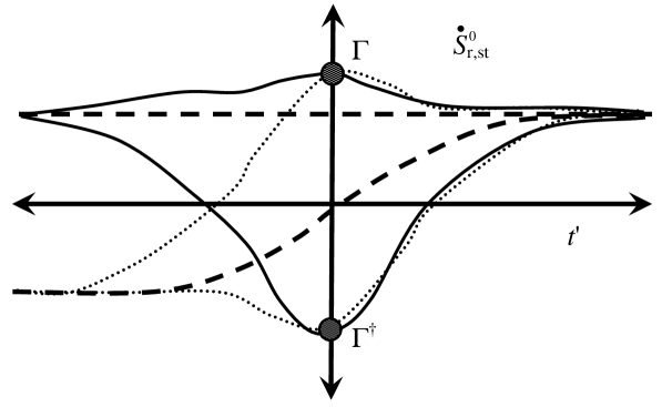
Figure 1: Sketch of $\dot{S}_{\mathrm{st}}^{0}$ for a steady state non-equilibrium system, in the future and in the past, starting from a likely phase space point ${\bf\Gamma}$, and from its unlikely conjugate ${\bf\Gamma}^{\dagger}$. The solid curves are on most likely trajectories, $\overline{\bf\Gamma}(t^{\prime}|{\bf\Gamma},0)$ and $\overline{\bf\Gamma}(t^{\prime}|{\bf\Gamma}^{\dagger},0)$, and the dotted curves are on adiabatic trajectories, ${\bf\Gamma}^{0}(t^{\prime}|{\bf\Gamma},0)$ and ${\bf\Gamma}^{0}(t^{\prime}|{\bf\Gamma}^{\dagger},0)$. The dashed line and curve are the respective asymptotes. From Ref. [NETDSM, ].

The behavior of the adiabatic rate of entropy production on various trajectories is sketched in Fig. 1. On the most likely trajectory the asymptotes are

$$\dot{S}_{\mathrm{st}}^{0}(\overline{\bf\Gamma}(t^{\prime}|{\bf\Gamma},t),t^{\prime})\rightarrow\overline{\dot{S}_{\mathrm{st}}^{0}}(t^{\prime}),\;\;|t^{\prime}-t|\rightarrow\infty.$$ (45)

This asymptote arises from the fact that with overwhelming probability the system came from its most likely value in the past (and will return there in the future), independent of the current phase space point of the sub-system. For a mechanical non-equilibrium system, the Hamiltonian has to be extended into the future, $\tilde{\cal H}({\bf\Gamma},t^{\prime};t)={\cal H}({\bf\Gamma},2t-t^{\prime})$ for $t^{\prime}>t$, and this causes the future asymptote to depend upon the current time, $\overline{\dot{S}_{\mathrm{st}}^{0}}(t^{\prime};t)$. This extended Hamiltonian is an even function of time about the current time $t$. For a steady state system, the asymptote is independent of $t^{\prime}$ and $t$.

In contrast, the asymptotic behavior on the adiabatic trajectory is

$$\dot{S}_{\mathrm{st}}^{0}({\bf\Gamma}^{0}(t^{\prime}|{\bf\Gamma},t),t^{\prime}) \sim \mbox{sign}(t^{\prime}-t)\,\overline{\dot{S}_{\mathrm{st}}^{0}}(t^{\prime}).$$ (46)

This holds for $|t^{\prime}-t|\gtrsim\tau_{\mathrm{relax}}$, where $\tau_{\mathrm{relax}}$ is a relaxation time that is long enough for the system to reach its asymptote, but not so long that the structure has changed significantly, $|\tau_{\mathrm{relax}}\dot{S}_{\mathrm{st}}^{0}|\ll|S_{\mathrm{st}}|$. (One does not need to impose this condition for the dissipative trajectory because the interactions with the reservoir maintain the structure of the sub-system.) For an isolated system, the structure represents a fluctuation, and $\dot{S}_{\mathrm{st}}^{0}$ represents its regression, which must be an odd function of time, at least for a steady state system. For $t^{\prime}>0$, the adiabatic asymptote and the actual asymptote approximately coincide, which is just Onsager’s regression hypothesis.Onsager31

In view of the trajectories shown in Fig. 1 and the above discussion, the odd projection of the dynamic part of the reservoir entropy may be transformed from an integral over the most likely trajectory to an integral over the adiabatic trajectories. Successive transformations yield

$$-2S_{\mathrm{dyn}}^{\mathrm{odd}}({\bf\Gamma},t)$$

$$= \int_{0}^{t}\mathrm{d}t^{\prime}\,\left[\dot{S}_{\mathrm{st}}^{0}(\overline{\bf\Gamma}(t^{\prime}|{\bf\Gamma},t),t^{\prime})-\dot{S}_{\mathrm{st}}^{0}(\overline{\bf\Gamma}(t^{\prime}|{\bf\Gamma}^{\dagger},t),t^{\prime})\right]$$

$$\approx \int_{t}^{2t}\mathrm{d}t^{\prime}\,\left[\dot{S}_{\mathrm{st}}^{0}(\overline{\bf\Gamma}(t^{\prime}|{\bf\Gamma},t),t^{\prime})-\dot{S}_{\mathrm{st}}^{0}(\overline{\bf\Gamma}(t^{\prime}|{\bf\Gamma}^{\dagger},t),t^{\prime})\right]$$

$$\approx \int_{t}^{2t}\!\mathrm{d}t^{\prime}\!\left[\dot{S}_{\mathrm{st}}^{0}({\bf\Gamma}^{0}(t^{\prime}|{\bf\Gamma},t),t^{\prime})-\dot{S}_{\mathrm{st}}^{0}({\bf\Gamma}^{0}(t^{\prime}|{\bf\Gamma}^{\dagger},t),t^{\prime})\right]$$

$$= \int_{0}^{t}\!\mathrm{d}t^{\prime}\!\left[\dot{S}_{\mathrm{st}}^{0}({\bf\Gamma}^{0}(t^{\prime}|{\bf\Gamma}^{\dagger},t)^{\dagger},t^{\prime})-\dot{S}_{\mathrm{st}}^{0}({\bf\Gamma}^{0}(t^{\prime}|{\bf\Gamma},t)^{\dagger},t^{\prime})\right].$$

The first equality is the area between the solid curves in the left half of the figure. The second equality is the area between the solid curves in the right half of the figure. This follows because the dissipation on the most likely trajectory is to a good approximation even in time. The third equality is the area between the dotted curves in the right half of the figure. This follows from Onsager’s regression hypothesis. The fourth equality is the area between the dotted curves in the left half of the figure. This follows from the time reversibility of Hamilton’s equations of motion,

$${\bf\Gamma}^{0}(t^{\prime}|{\bf\Gamma}^{\dagger},t)={\bf\Gamma}^{0}(2t-t^{\prime}|{\bf\Gamma},t)^{\dagger}.$$ (48)

For a mechanical non-equilibrium system, the extended system Hamiltonian preserves this property.

For a thermodynamic, steady state, non-equilibrium system, the adiabatic rate of change of the static part of the reservoir entropy is $\dot{S}_{\mathrm{st}}^{0}({\bf\Gamma})=\dot{\bf\Gamma}^{0}\cdot\nabla S_{\mathrm{st}}({\bf\Gamma})$, and this has odd parity, $\dot{S}_{\mathrm{st}}^{0}({\bf\Gamma}^{\dagger})=-\dot{S}_{\mathrm{st}}^{0}({\bf\Gamma})$. (For time varying, reservoir induced, thermodynamic gradients (i.e. non steady state), $\dot{S}_{\mathrm{st}}^{0}({\bf\Gamma},t)$ is of mixed parity.) For a mechanical non-equilibrium system, the adiabatic rate of change of the static part of the reservoir entropy is $\dot{S}_{\mathrm{st}}^{0}({\bf\Gamma},t)=-T^{-1}\partial U^{\mathrm{ext}}({\bf\Gamma},t)/\partial t$, and this has even parity, $\dot{S}_{\mathrm{st}}^{0}({\bf\Gamma}^{\dagger})=\dot{S}_{\mathrm{st}}^{0}({\bf\Gamma})$. Accordingly one can take the conjugate of the trajectories in the final equality of the above expression for the dynamic part of the reservoir entropy and define

$$S_{\mathrm{dyn}}^{\mathrm{odd;0}}({\bf\Gamma},t) \equiv \frac{-1}{2}\int_{0}^{t}\!\mathrm{d}t^{\prime}\!\left[\dot{S}_{\mathrm{st}}^{0}({\bf\Gamma}^{0}(t^{\prime}|{\bf\Gamma},t),t^{\prime})\right.$$ (49)

$$\left.\mbox{ }-\dot{S}_{\mathrm{st}}^{0}({\bf\Gamma}^{0}(t^{\prime}|{\bf\Gamma}^{\dagger},t),t^{\prime})\right].$$

In these two cases one has

$$S_{\mathrm{dyn}}^{\mathrm{odd}}({\bf\Gamma},t)=\pm S_{\mathrm{dyn}}^{\mathrm{odd;0}}({\bf\Gamma},t),$$ (50)

with the positive sign applying to a thermodynamic, steady state, non-equilibrium system, and the negative sign applying to a mechanical non-equilibrium system. The left hand side invokes backward most likely trajectories, and the right hand side invokes backward adiabatic trajectories.

It is obvious from the figure that the integrand asymptotes to zero. This means that the lower limit of the integral can be replaced by $t-\tau$ for some convenient interval $\tau>0$. Although the integrand is an exact differential, there is no point in analytically evaluating the integral because the actual value at the lower limit would be required, $S_{\mathrm{dyn}}^{\mathrm{odd}}({\bf\Gamma},t)=\pm[S_{\mathrm{st}}({\bf\Gamma}^{0}(t-\tau|{\bf\Gamma},t),t-\tau)-S_{\mathrm{st}}({\bf\Gamma}^{0}(t-\tau|{\bf\Gamma}^{\dagger},t),t-\tau)]/2$. (Although $\dot{S}_{\mathrm{st}}^{0}$ has the same asymptote starting at ${\bf\Gamma}$ and at ${\bf\Gamma}^{\dagger}$, there is a finite difference between the respective asymptotes of $S_{\mathrm{st}}$ that corresponds to the area between the two curves in the left half of the figure.) It takes no more computational effort to perform the quadrature numerically than it does to calculate the adiabatic trajectories backward to their lower limit.

In summary, this section argues that in some circumstances the odd projection of the dynamic part of the reservoir entropy is either dominant or is all that is required. Further it says that the odd projection of the dynamic part of the reservoir entropy may be evaluated on the past adiabatic trajectories. With this result, one does not need to evaluate the most likely backwards trajectory, and hence one does not need $\overline{\bf R}({\bf\Gamma},\Delta_{t},t)$, for $\Delta_{t}<0$. This means that explicit knowledge of $\overline{\bf\Gamma}(t)$ is not required, which is a great advantage. As mentioned at the beginning of this section, this adiabatic expression for the dynamic part of the reservoir entropy has been tested with computer simulations of both mechanical and thermodynamic non-equilibrium systems and it has been found to be accurate.

IV.0.1 Green-Kubo Relations

The validity and utility of the expression for the non-equilibrium probability will now be illustrated with a simple derivation of the Green-Kubo relations. Onsager31 ; Green54 ; Kubo66 These relate the hydrodynamic transport coefficients to the equilibrium time correlation functions of the fluxes.

For the particular case of heat flow, the static part of the reservoir entropy isNETDSM ; AttardI

$$S_{\mathrm{st}}({\bf\Gamma})=\frac{-E_{0}({\bf\Gamma})}{T_{0}}-\frac{E_{1}({\bf\Gamma})}{T_{1}},$$ (51)

where the $n$th energy moment in the $z$-direction is $E_{n}({\bf\Gamma})\equiv\int\mathrm{d}{\bf r}\,\epsilon({\bf r};{\bf\Gamma})z^{n}$, with $\epsilon({\bf r};{\bf\Gamma})$ being the energy density at ${\bf r}$. Also the zeroth temperature is the mid-temperature of the two reservoirs, $T_{0}^{-1}\equiv[T_{+}^{-1}+T_{-}^{-1}]/2=T^{-1}+{\cal O}(\nabla T)^{2}$, and the first temperature is essentially the temperature gradient imposed by them, $T_{1}^{-1}\equiv[T_{+}^{-1}-T_{-}^{-1}]/L_{z}=-T^{-2}\nabla T+{\cal O}(\nabla T)^{2}$.

The instantaneous heat flux, a phase function of the isolated sub-system, is essentially the adiabatic rate of change of the first energy moment, Onsager31 ; NETDSM ; AttardI

$$J_{\mathrm{E}}({\bf\Gamma})\equiv\dot{E}_{1}^{0}({\bf\Gamma})/V,$$ (52)

where $V$ is the volume of the sub-system. Due to energy conservation of the isolated system, $\dot{E}_{0}^{0}({\bf\Gamma})=0$ and $\dot{S}^{0}_{\mathrm{st}}({\bf\Gamma})=-\dot{E}_{1}^{0}({\bf\Gamma})/T_{1}$.

Fourier’s law gives the heat flow in the presence of an applied thermal gradient, and it is Kubo78 ; Zwanzig01 ; Bellac04 ; Pottier10 ; NETDSM

$$\overline{J}_{\mathrm{E}}=-\lambda\nabla T,$$ (53)

where $\lambda$ is the thermal conductivity. The left hand side is the most likely heat flux, which equals the average heat flux. This law of course holds to linear order in the temperature gradient.

The average heat flux given by the present non-equilibrium theory is

$$\left<J_{\mathrm{E}}\right>_{\mathrm{non-equil}}$$ (54)

$$= \frac{1}{V}\int\mathrm{d}{\bf\Gamma}\;\wp({\bf\Gamma}|T_{0},T_{1})\dot{E}_{1}^{0}({\bf\Gamma})$$

$$= \frac{1}{V}\frac{\int\mathrm{d}{\bf\Gamma}\;e^{[S_{\mathrm{st}}({\bf\Gamma})+S_{\mathrm{dyn}}({\bf\Gamma})]/k_{\mathrm{B}}}\dot{E}_{1}^{0}({\bf\Gamma})}{\int\mathrm{d}{\bf\Gamma}\;e^{[S_{\mathrm{st}}({\bf\Gamma})+S_{\mathrm{dyn}}({\bf\Gamma})]/k_{\mathrm{B}}}}$$

$$= \frac{1}{Vk_{\mathrm{B}}}\frac{\int\mathrm{d}{\bf\Gamma}\;e^{-E_{0}({\bf\Gamma})/k_{\mathrm{B}}T_{0}}\dot{E}_{1}^{0}({\bf\Gamma})S_{\mathrm{dyn}}^{\mathrm{odd;0}}({\bf\Gamma})}{\int\mathrm{d}{\bf\Gamma}\;e^{-E_{0}({\bf\Gamma})/k_{\mathrm{B}}T_{0}}}+{\cal O}(\nabla T)^{2}$$

$$= \frac{1}{2Vk_{\mathrm{B}}T_{1}}\int_{-\tau}^{0}\mathrm{d}t^{\prime}\,\left<\dot{E}_{1}^{0}({\bf\Gamma})\left[\dot{E}_{1}^{0}({\bf\Gamma}^{0}(t^{\prime}|{\bf\Gamma},0)\right.\right.$$

$$\left.\left.\mbox{ }-\dot{E}_{1}^{0}({\bf\Gamma}^{0}(t^{\prime}|{\bf\Gamma}^{\dagger},0)\right]\right>_{\mathrm{equil}}$$

$$= \frac{-\nabla T}{2Vk_{\mathrm{B}}T_{0}^{2}}\int_{-\tau}^{\tau}\mathrm{d}t^{\prime}\,\left<\dot{E}_{1}^{0}({\bf\Gamma})\dot{E}_{1}^{0}({\bf\Gamma}^{0}(t^{\prime}|{\bf\Gamma},0)\right>_{\mathrm{equil}}.$$

In the third equality the exponentials have been expanded in powers of the temperature gradient and second order terms have been neglected. As well, terms that are the product of an even parity function, $S_{\mathrm{st}}({\bf\Gamma})$ or $S_{\mathrm{dyn}}^{\mathrm{even}}({\bf\Gamma})$, and an odd parity function, $\dot{S}_{\mathrm{st}}^{0}({\bf\Gamma})$ or $\dot{E}_{1}^{0}({\bf\Gamma})$, vanish upon integration over phase space. In addition, the most likely trajectory has been replaced by the adiabatic trajectory, Eq. (50). The equilibrium average arises because $Z(T_{0})^{-1}e^{-E_{0}({\bf\Gamma})/k_{\mathrm{B}}T_{0}}$ is the Maxwell-Boltzmann distribution. Comparing this to Fourier’s law, one can identify the thermal conductivity as

$$\lambda = \frac{1}{2k_{\mathrm{B}}VT_{0}^{2}}\int_{-\tau}^{\tau}\mathrm{d}t^{\prime}\,\left<E_{1}^{0}({\bf\Gamma})\dot{E}_{1}^{0}({\bf\Gamma}^{0}(t^{\prime}|{\bf\Gamma},0)\right>_{\mathrm{equil}}$$ (55)

$$= \frac{1}{2Vk_{\mathrm{B}}T_{0}^{2}}\left<\dot{E}_{1}^{0}(t)\left[E_{1}(t+\tau)-E_{1}(t-\tau)\right]\right>_{\mathrm{equil}}.$$

The right hand side is independent of $\tau$ for for $\tau\gtrsim\tau_{\mathrm{relax}}$. This can be written in a number of different ways, but all involve the equilibrium time correlation function of the heat flux or an integral thereof. This is a typical example of a Green-Kubo relation. Onsager31 ; Green54 ; Kubo66 It is to be noted that the time correlation function in any Green-Kubo relation always invokes adiabatic trajectories. Kubo78 ; Zwanzig01 ; Bellac04 ; Pottier10 ; NETDSM

From this analysis one sees that the general formula for obtaining the Green-Kubo relations is

$$\left<\dot{S}_{\mathrm{st}}^{0}({\bf\Gamma})\right>_{\mathrm{non-equil}}$$ (56)

$$= \frac{\pm 1}{k_{\mathrm{B}}}\left<\dot{S}_{\mathrm{st}}^{0}({\bf\Gamma})\,S_{\mathrm{dyn}}^{\mathrm{odd;0}}({\bf\Gamma})\right>_{\mathrm{equil}},$$

with the plus sign for steady state thermodynamic systems, and the minus sign for mechanical non-equilibrium systems. The fact that the theory gives the Green-Kubo relations should give one confidence both in the adiabatic transformation of the dynamic part of the reservoir entropy, Eq. (50), and in the general expression for the phase space probability for non-equilibrium systems, Eq. (11). Of course the Green-Kubo relations are a linear theory, whereas the present expression for the phase space probability for non-equilibrium systems applies in all circumstances, linear and non-linear.

Conclusion

The non-equilibrium phase space probability distribution, Eq. (11),

$$\wp({\bf\Gamma},t)=\frac{1}{Z(t)}e^{S_{\mathrm{r}}({\bf\Gamma},t)/k_{\mathrm{B}}},$$

is simply a formal statement that probability is the exponential of the total entropy, which equals the reservoir entropy because the points in the phase space of the sub-system have no internal entropy. This is formally the same as in the equilibrium case. The specifically non-equilibrium concept is that the reservoir entropy consists of a static and a dynamic part, Eq. (I.2),

$$S_{\mathrm{r}}({\bf\Gamma},t) = S_{\mathrm{st}}({\bf\Gamma},t)+S_{\mathrm{dyn}}({\bf\Gamma},t)$$

$$\equiv S_{\mathrm{st}}({\bf\Gamma},t)-\int_{0}^{t}\mathrm{d}t^{\prime}\,\dot{S}_{\mathrm{st}}^{0}(\overline{\bf\Gamma}(t^{\prime}|{\bf\Gamma},t),t^{\prime}).$$

The static part is the ordinary equilibrium expression that is based on exchange of conserved variables with the reservoir. In a non-equilibrium system the conservation laws may not hold, (e.g. the energy may change due to a time-varying external potential, or energy gradients may change by internal relaxation processes), and so the dynamic part of the reservoir entropy subtracts the adiabatic or internal change from the total change. This adiabatic change is path dependent, but in the thermodynamic limit it can be obtained by integrating over the most likely trajectory leading to the current point and neglecting fluctuations about this trajectory. In §IV a useful adiabatic approximation to the trajectory used in the dynamic part of the entropy was given.

In §§II and III the stochastic, dissipative equations of motion that correspond to this non-equilibrium probability density were given. For a single time step, the phase space transition $\{{\bf\Gamma}_{1},t_{1}\}\rightarrow\{{\bf\Gamma}_{2},t_{2}\}$ was found to be governed by the stochastic, dissipative equation (40),

$${\bf\Gamma}_{2} = {\bf\Gamma}_{1}+t_{21}\dot{\bf\Gamma}^{0}+\frac{|t_{21}|}{2}\Lambda(t)\cdot\nabla S_{\mathrm{st}}({\bf\Gamma},t)$$

$$\mbox{ }+\frac{t_{21}-|t_{21}|}{2}\Lambda(t)\cdot\nabla S_{\mathrm{st}}(\overline{\bf\Gamma}(t),t)+\tilde{\bf R}(|t_{21}|,t).$$

There are four transition terms on the right hand side.

The first term is the adiabatic velocity, which is due to the internal interactions within the sub-system, and which would occur if it were isolated. These are of course reversible (proportional to $t_{21}$).

The second term represents some of the reservoir forces on the sub-system. These are driven by the change in reservoir entropy due to the sub-system–reservoir interactions. It is $S_{\mathrm{st}}$ not $S_{\mathrm{r}}$ that accounts for the change in entropy due to the exchange of conserved variables between the sub-system and the reservoir. This exchange is of course carried by such interactions. Hence the gradient of the static part of the reservoir entropy provides the thermodynamic driving force for the transition. The drag coefficient $\Lambda(t)$ represents the strength of the statistical coupling between the sub-system and the reservoir. The thermodynamic gradient is toward the state of higher entropy, and as such it applies both forward and backward in time, (i.e. it is irreversible, $\propto|t_{21}|$).

The form of this second term arose in the thermodynamic gradient in Eq. (31) where the fluctuation matrix for the total reservoir entropy was approximated by that of the static part alone, Eq. (14),

$$\overline{S^{\prime\prime}}_{\mathrm{\!\!\!\!r}}\,(t)\approx\overline{S^{\prime\prime}}_{\mathrm{\!\!\!\!st}}(t),\mbox{ and }\overline{S^{\prime\prime}}_{\mathrm{\!\!\!\!dyn}}(t)\approx 0.$$

To the two original justifications for this approximation (that fluctuations about the non-equilibrium state are determined by the current molecular structure, and that these fluctuations have the same symmetries as equilibrium fluctuations) may now be added a third: it is essential that the thermodynamic driving force be $\nabla S_{\mathrm{st}}({\bf\Gamma},t)$ not $\nabla S_{\mathrm{r}}({\bf\Gamma},t)$, since the former gives the change in entropy specifically due to interactions and exchange between the sub-system and the reservoir.

The third term is basically the second term evaluated on the most likely trajectory, $\overline{\bf\Gamma}(t)$. This term arises as a correction to the second term because by definition the most likely trajectory is reversible (i.e. a single valued function of time can be chosen). One can see that on the most likely trajectory the irreversible parts of the second and third terms cancel with each other leaving the deterministic transition on this trajectory fully reversible. For a forward trajectory, $t_{21}>0$, the coefficient of this third term vanishes.

The fourth term is the stochastic term. It arises from the fact that the sub-system phase space is a projection of the total system phase space, and so the evolution of a trajectory in the sub-system is not uniquely determined by a point in the sub-system, which is the definition of randomness. The random force has zero mean, $\langle\tilde{\bf R}\rangle=0$. In the text the fluctuation form of the second entropy showed that it had variance, Eq. (39),

$$\left<\tilde{\bf R}(t)\,\tilde{\bf R}(t)\right>=|t_{21}|k_{\mathrm{B}}\Lambda(t).$$

This is the fluctuation-dissipation theorem. The magnitude and functional form of the drag coefficient $\Lambda(t)$ have little effect on the statistical results provided that the fluctuation-dissipation theorem is satisfied. With it the non-equilibrium probability is functionally stationary under the evolution governed by the stochastic, dissipative equations of motion (see §8.3.5 of Ref. [NETDSM, ]).

References

- (1) Feynman, R. P. (1998), Statistical Mechanics: Statistical Mechanics: A Set Of Lectures, (Advanced Books Classics, Westview Press, 2nd ed.).
- (2) Pathria, R. K. (1972), Statistical Mecahnics, (Pergamon Press, Oxford).
- (3) McQuarrie, D. A. (2000), Statistical Mecahnics, (University Science Books, Sausalito)
- (4) Attard, P. (2002), Thermodynamics and Statistical Mechanics: Equilibrium by Entropy Maximisation, (Academic Press, London).
- (5) Kubo, R., Toda, M., and Hashitsume, N. (1978), Statistical Physics II. Non-equilibrium Statistical Mechanics, (Springer-Verlag, Berlin).
- (6) Zwanzig, R. (2001), Non-equilibrium Statistical Mechanics, (Oxford University Press, Oxford).
- (7) Le Bellac, M., Mortessagne, F., and Batrouni, G. G., (2004), Equilibrium and Non-equilibrium Statistical Thermodynamics, (Cambridge University Press, Cambridge).
- (8) Pottier, N. (2010), Non-equilibrium Statistical Physics: Linear Irreversible Processes, (Oxford University Press, Oxford).
- (9) Attard, P. (2012), Non-Equilibrium Thermodynamics and Statistical Mechanics: Foundations and Applications, (Oxford University Press, Oxford).
- (10) Yamada, T. and Kawasaki, K. (1967), Progr. Theor. Phys. 38, 1031.
- (11) Yamada, T. and Kawasaki, K. (1975), Prog. Theo. Phys. 53, 111.
- (12) Attard, P. (2006), J. Chem. Phys. 124, 224103.
- (13) Attard, P. and Gray-Weale, A. (2008), J. Chem. Phys. 128, 114509.
- (14) Attard, P. (2009), J. Chem. Phys. 130, 194113.
- (15) Attard, P. (2009), Phys. Rev. E 80, 041126.
- (16) Attard, P. (2014), “Quantum Statistical Mechanics. IV. Non-Equilibrium Probability Operator”, arXiv: …
- (17) Onsager, L. (1931), Phys. Rev. 37, 405, and 38, 2265.
- (18) Green, M. S. (1954), J. Chem. Phys. 22, 398.
- (19) Kubo, R. (1966), Rep. Progr. Phys. 29, 255.
- (20) Attard, P. (2004), J. Chem. Phys. 121, 7076.