Superflare occurrence and energies on G, K and M type dwarfs

Abstract

Kepler data from G-, K-, and M-type stars are used to study conditions that lead to superflares with energies above $10^{34}{\rm erg}$. From the 117,661 stars included, 380 show superflares with a total of 1690 such events. We study whether parameters, like effective temperature or rotation rate, have any effect on the superflare occurrence rate or energy. With increasing effective temperature we observe a decrease in the superflare rate, which is analogous to the previous findings of a decrease in dynamo activity with increasing effective temperature. For slowly rotating stars, we find a quadratic increase of the mean occurrence rate with the rotation rate up to a critical point, after which the rate decreases linearly. Motivated by standard dynamo theory, we study the behavior of the relative starspot coverage, approximated as the relative brightness variation. For faster rotating stars, an increased fraction of stars shows higher spot coverage, which leads to higher superflare rates. A turbulent dynamo is used to study the dependence of the Ohmic dissipation as a proxy of the flare energy on the differential rotation or shear rate. The resulting statistics of the dissipation energy as a function of dynamo number is similar to the observed flare statistics as a function of the inverse Rossby number and shows similarly strong fluctuations. This supports the idea that superflares might well be possible for solar-type G stars.

2014 August 18

1. Introduction

Research in solar and stellar variability has often focused on grand minima, but seldom on grand maxima. One of the characteristics of a grand maximum may be an enhanced frequency of superflares. Superflares release energies of $10^{34}\,{\rm erg}$ or more. Such flares are not generally expected to occur in the Sun, where the strongest flares have only about $10^{32}\,{\rm erg}$; an example of this is the Carrington flare of 1859 (Carrington, 1859; Hodgson, 1859).

Exhaustive statistics of superflares in other solar-like stars with solar rotation rates (Maehara et al., 2012; Shibayama et al., 2013; Nogami et al., 2014) have reinvigorated the discussion of whether or not such events could in principle also occur in the Sun. Of particular importance is the realization that “hot Jupiters” are not required (Shibata et al., 2013; Shibayama et al., 2013), contrary to what was previously believed (Schaefer et al., 2000). The recent work of Shibata et al. (2013) explored the possible connection between flare intensity and sunspot area. They argue that flux transport dynamos (Choudhuri et al., 1995; Dikpati & Charbonneau, 1999; Nandy & Choudhuri, 2002) might be capable of generating enough magnetic flux, storing it beneath the convection zone for some time, and then releasing it in a violent eruption. One of the aims of the present paper is to find favorable conditions under which superflares can occur. We will discuss an alternative scenario for the origin of superflares within the framework of turbulent dynamo theory.

Dynamo activity is connected to stellar rotation through the dependence of the $\alpha$ effect and shear on the rotation rate. Both quantities are important ingredients in large-scale dynamos, where the $\alpha$ effect is necessary in most dynamo models (Steenbeck et al., 1966; Pouquet et al., 1976; Brandenburg & Subramanian, 2005). A positive correlation between the star’s rotation rate and the occurrence of superflares is therefore expected.

It is generally believed that as the star’s magnetic energy increases, more and larger starspots can occur. We expect that this excess magnetic energy is stored until the spot dissolves or magnetic reconnection initiates a flare (Su et al., 2013; Malanushenko et al., 2014). Individual flare events can only be resolved for the Sun. For distant stars, they need to be inferred by characteristic brightness variations. Maehara et al. (2012) found 148 stars with 365 such events by searching for peaks in the light curves from data compiled by the Kepler mission (Koch et al., 2010). Subsequent work by the same group (Shibayama et al., 2013) extended the number of stars to 279 and flare events to 1547.

Starspots are manifested through periodic variations of a star’s luminosity. From past work we know that inferring spot coverage or spot size from light curves is accompanied by large uncertainties (Kovari & Bartus, 1997). Therefore, we perform calculations for the brightness variations of model stars for which we know the spot distribution and measure the statistical spread.

Dynamo theory describes the conversion of kinetic energy into magnetic energy. In late-type stars such as the Sun, the kinetic energy comes from convection in the outer layers. Since flares are associated with magnetic fields, it seems clear that the cause of superflares should be explicable in terms of dynamo theory. Dynamo theory is a broad subject encompassing both small-scale and large-scale dynamos. Usually, only the large-scale dynamo is associated with the solar cycle, but small-scale dynamo action might well occur at the same time. In fact, at small scales, the two cannot even be distinguished, because their magnetic and kinetic power spectra are virtually the same (Brandenburg et al., 2012).

It is conceivable that flare activity is more directly related to the small-scale part of turbulence. Indeed, only at small length scales does hydrodynamic and hydromagnetic turbulence display the characteristics of strong intermittency with bursts and long waiting times (Veltri et al., 2005), required to explain a broad range of different flares, including superflares. On the other hand, both flares and coronal mass ejections may also be associated with magnetic helicity (Schrijver, 2009), whose long-term variability is certainly a feature of large-scale dynamos. Superflares might therefore be the result of the simultaneous occurrence of two or more time-dependent stochastic events.

2. Flare Activity, Rotation, and Temperature

EUV images of the Sun have long revealed the presence of magnetically confined hot plasma. Thermal X-ray emission from such hot plasma therefore provides proxies of magnetic activity (Pallavicini et al., 1981; Walter, 1982; Vilhu, 1984) which are all correlated with the Coriolis or inverse Rossby number, $\mbox{\rm Ro}^{-1}=\tau/P_{\rm rot}$, where $P_{\rm rot}$ is the rotation period and $\tau$ is the convective turnover time. To check whether superflare activity also correlates with $\mbox{\rm Ro}^{-1}$, we consider the set of superflare stars identified by Maehara et al. (2012), which was subsequently extended to quarters 0 to 6 of the Kepler survey (Koch et al., 2010) with 380 superflare stars, 373 of which have a well-determined rotation period.

We consider the superflare frequency $\nu$, which is the number of superflares per unit time. Here, a superflare is defined as an event that releases a total energy of $5\times 10^{34}\,{\rm erg}$ or more within a few hours. Of the updated sample of Maehara et al. (2012), there are 129 G-type stars with effective temperatures in the range $5200\,{\rm K}\leq T_{\rm eff}<6000\,{\rm K}$, 227 K-type stars with $3700\,{\rm K}\leq T_{\rm eff}<5200\,{\rm K}$, and 17 M-type stars with $2400\,{\rm K}\leq T_{\rm eff}<3700\,{\rm K}$. To determine their Rossby numbers, we use the empirically determined turnover times $\tau$ of Noyes et al. (1984), who found a relation between $\tau$ and the $B-V$ color.

In Figure 1, we plot the dimensional and non-dimensional superflare frequencies, $\nu$ and $\nu\tau$ versus $T_{\rm eff}$. We see that the superflare rate is uniformly distributed and nearly independent of the star’s effective temperature. We further plot $\nu\tau$ versus $\mbox{\rm Ro}^{-1}$ (Figure 2). It turns out that there is no clear correlation between $\nu\tau$ and $\mbox{\rm Ro}^{-1}$, as can also be seen from the nearly flat profile of the green line in Figure 2, which shows the average taken over all superflaring stars within the shown interval in ${\rm Ro}^{-1}$.

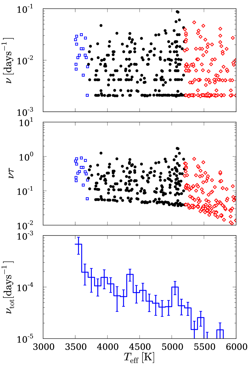
Figure 1.— Unnormalized flare frequency $\nu$ vs. $T_{\rm eff}$ (upper panel), normalized $\nu\tau$ (central panel) and binned averages for the flare frequency $\nu_{\rm tot}$ including non-superflaring stars (lower panel). Blue squares refer to M-type stars (effective temperatures below $T_{1}=3700\,{\rm K}$) and red diamonds to G-type stars (temperatures above $T_{2}=5200\,{\rm K}$). Black dots refer to K-type stars (temperatures between $T_{1}$ and $T_{2}$). The lower cutoff in $\nu$ is $\nu_{\min}=1/t_{\max}$ and is an artifact of the finite length of the observed time series, $t_{\max}$.

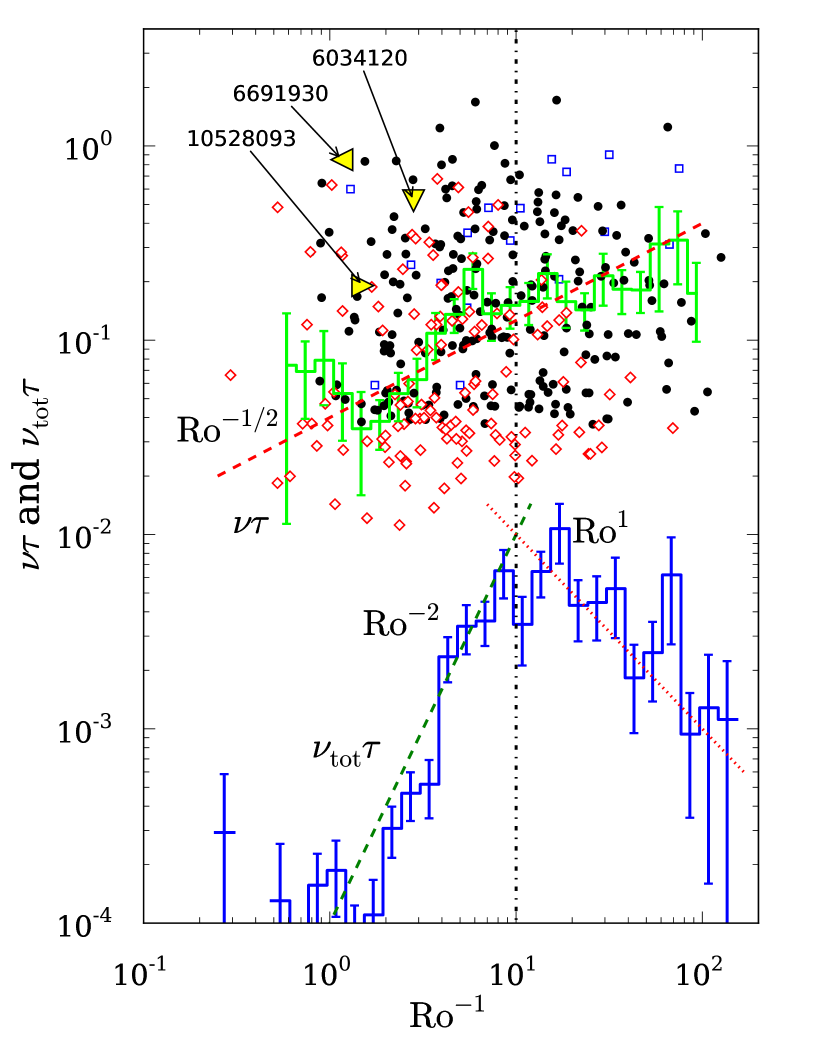
Figure 2.— Non-dimensional flare frequency $\nu\tau$ vs. $\mbox{\rm Ro}^{-1}=\tau/P_{\rm rot}$. Color and shape coding of the markers are the same as in Figure 1. The stars considered in Notsu et al. (2013) are highlighted as yellow triangles, together with their Kepler ID. The upper (green) curve shows the averaged superflare frequencies for intervals in $\mbox{\rm Ro}^{-1}$ including only superflaring stars. From the seemingly random scatter plot and the flat profile for the averaged $\nu\tau$, it becomes clear that there is no correlation between $\mbox{\rm Ro}^{-1}$ and $\nu\tau$. In contrast, the lower (blue) plot shows the average value of $\nu_{\rm tot}\tau$ (which includes non-superflaring stars) as a function of the inverse Rossby number. There, two regimes can be distinguished. For $\mbox{\rm Ro}^{-1}\lesssim 10$, we find a power law of $-2$, while for higher values we find $1$ for the power.

Note that the analysis above only includes stars which showed superflares during the observation period. Such an analysis does not give any hint as to whether or not all stars with specific parameters, like the Rossby number, are more likely to produce superflares. By normalizing with respect to all observed Kepler stars from quarters 0 to 6, we compute the average superflare occurrence rate, $\nu_{\rm tot}$, over a set of binning intervals where we include both superflaring and non-superflaring stars (the total number of those stars is 117,661, only 115,984 of which with a well defined rotation period were included). We find a clear decrease of the superflare frequency $\nu_{\rm tot}$ with increasing effective temperature (Figure 1, lower panel). This might seem to be in contradiction with observational results showing a clear positive power-law dependence of the surface shear on the effective temperature (Barnes et al., 2005). Subsequent model calculations, however, showed that for hotter stars, eddy diffusion increases such that it overcompensates for the increase in shear which leads to a reduced dynamo number (Kitchatinov & Olemskoy, 2011), thus explaining our results.

For the Rossby number dependence, we find two regimes separated by a boundary at $\mbox{\rm Ro}^{-1}\approx 10$. For lower values, the superflare occurrence rate shows a power law proportional to $\mbox{\rm Ro}^{-2}$, while for higher $\mbox{\rm Ro}^{-1}$ we find a $\mbox{\rm Ro}^{1}$ behavior (Figure 2, lower curve). With a total of 373 superflaring stars, we have confidence in the validity of our statistical analysis. Furthermore, the determined power laws fit the computed averages remarkably well.

The position of the break at $\mbox{\rm Ro}^{-1}\approx 10$ agrees with the well-known point of saturation of chromospheric and X-ray activity for large values of $\mbox{\rm Ro}^{-1}$ (see, e.g. Pizzolato et al., 2003; Wright et al., 2011). For smaller values of $\mbox{\rm Ro}^{-1}$, they find an approximately quadratic increase of X-ray luminosity, which is similar to our quadratic increase of flare frequency. At larger values of $\mbox{\rm Ro}^{-1}$, stellar activity is saturated and thus not compatible with the fall-off seen in the lower curve of Figure 2.

3. Relation to Starspots

3.1. Relative Star Population

Enhanced magnetic activity is manifested through the increased occurrence of starspots. Starspots can be inferred through cyclic variations in the light curves with frequencies equal to the rotation frequency. For every star, we know its relative flux variation $\Delta F/F_{\rm av}$ (Maehara et al., 2012), where $\Delta F$ is the range over which the flux varies and $F_{\rm av}$ is the averaged flux. According to Koch et al. (2010), the shot noise for stars measured over 6.5 hr is 14 ppm, which will be our detection limit for $\Delta F/F_{\rm av}$. We use this as proxy for the fraction of the stellar surface covered by spots. In principle, there can be other causes for the observed flux variation, e.g., differential rotation (Reinhold et al., 2013) and exoplanets, but the latter were excluded by Maehara et al. (2012). Furthermore, starspots which are visible during a whole revolution, like those spots extending over the poles, would weaken the applicability of the flux variation as a proxy for starspot coverage, since they would constantly reduce the flux. A thorough study of the observational bias is presented in Section 4.

We expect enhanced dynamo activity and larger and more starspots for rapidly rotating stars, i.e., for large values of $\mbox{\rm Ro}^{-1}$. This is reflected in the dependence of the relative flux variation for the 115,984 stars in this catalog (Figure 3, one-dimensional (1D) histogram), where we plot the average of $\Delta F/F_{\rm av}$ for certain intervals of $\mbox{\rm Ro}^{-1}$. Apart from two outliers, we obtain good agreement with a power-law dependence of $\Delta F/F_{\rm av}\propto\mbox{\rm Ro}^{-1/2}$. Analytical mean-field dynamo calculations and simulations for rotating shearing dynamo models (Karak et al., 2014) have shown that the saturation magnetic field strength increases with the rotation frequency $\Omega$ with a power law of $\mbox{\rm Ro}^{-1/2}$, which is in agreement with the observations.

Kepler observations cover stars at a random phase of their magnetic activity cycle. During low magnetic activity, very few starspots are expected, independent of the Rossby number. During high magnetic activity, strong flux variations are expected. Those variations can depend well on the rotation rate, as dynamo activity is expected to increase with $\mbox{\rm Ro}^{-1}$. Those two branches of low and high magnetic activity can be seen in Figure 3 (color mapping), where we plot a two-dimensional probability distribution for stars showing a brightness variation and Rossby number in a certain interval. The two regimes are clearly visible, where for one there is no Ro dependence, while for the other we observe $\Delta F/F_{\rm av}\propto\mbox{\rm Ro}^{-2}$ for $\mbox{\rm Ro}^{-1}\lesssim 3.2$ and a constant for $\mbox{\rm Ro}^{-1}\gtrsim 3.2$.

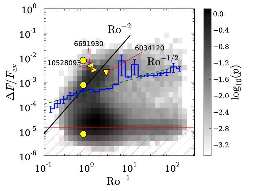
Figure 3.— Average value of $\Delta F/F_{\rm av}$ dependent on the Rossby number including all observed 115,984 stars (1D histogram). Probability distribution function for the same set of stars dependent on $\Delta F/F_{\rm av}$ and $\mbox{\rm Ro}^{-1}$ (color mapping). The hatched area indicates the detection limit. Standard dynamo predictions for which magnetic activity is expected to increase with rotation rate (Karak et al., 2014) are confirmed for this set of stars, provided the relative flux variation is a good proxy for the total magnetic flux. Apart from a general increase of the relative brightness variation, we observe two regimes (darker shades). The upper regime can be identified as the active regime where the stars were magnetically active during the observation. Here, one observes an increase of the flux variation as the rotation rate increases. For the stars in their magnetic minima, rotation does not play any role. Three particular superflaring stars investigated in Notsu et al. (2013) are highlighted here as yellow triangles together with their Kepler ID. The strong brightness variation of those three stars indicates large spots which can trigger superflares, as seen in Figure 2. For comparison, we also indicate the Sun’s position in this diagram if it was covered with sunspots for 1%, 0.1%, and 0.001% (upper, middle, and lower yellow circle, respectively).

3.2. Sunspot Coverage Since 1874

The Sun’s cyclic variations and historic grand minima show that magnetic activity can exhibit significant long-term variability. There is no reason to attribute these characteristics exclusively to our nearest star. Other stars may have been in phases of high and low magnetic activity during Kepler’s observations. The Kepler mission, with its 90-500 days observing time, will have observed stellar brightness at random phases, and hence starspot coverages. This can explain the two regimes in Figure 3. As the stars included here are all solar like, we should expect to observe the Sun in either regime for a long enough observation interval. Judging from Figure 3, there is a significant chance that the Sun will be in the upper or lower regimes, while the area in between is unlikely to be observable.

Using the data of Hathaway, we know the sunspot coverage of the visible hemisphere from 1874 May until 2013 July, with a time resolution of one day and only a few short intervals with no observations. From that data set, we compute the brightness variation. The sunspot temperature is taken to be $T_{\rm s}=4000\,{\rm K}$, while $T_{\rm p}=5800{\rm K}$ is assumed for the photospheric temperature. According to Notsu et al. (2013), the brightness variation is calculated as

$$\Delta F/F_{\rm av}=\left(1-(T_{\rm s}/T_{\rm p})^{4}\right)\times q,$$ (1)

where $q$ is the relative sunspot coverage. Any bright magnetic structures, which tend to exist on small scales, would contribute to the total magnetic energy while decreasing $\Delta F/F_{\rm av}$. Since those are not included in the catalog for the Sun, we disregard such structures in our calculations. It has been found, however, that the Sun increases in irradiance by approximately $1\%$ during high magnetic activity and high sunspot number (Fröhlich & Lean, 1998). This effect was attributed to facular brightening which overcompensates the darkening effect from the sunspots. As as faculae are much more homogeneously distributed over the Sun, they do not lead to significant brightness variations on timescales of the order of one rotation period. As Kepler observation times are much shorter than the magnetic cycle period, the enhanced brightness appears as increased background radiation and does not affect Equation (1). Variations in irradiance on timescales of days (Willson & Hudson, 1981), on the other hand, were attributed to the appearance of sunspot groups (Willson et al., 1981), hence justifying our model.

The probability distribution function for finding the brightness variation $\Delta F/F_{\rm av}$ at any time between 1874 May and 2013 July shows an exponential shape (Figure 4), unlike the expected two regimes with high probability for high and low brightness variation. As the spot coverage of the superflaring stars is higher than has ever been observed for the Sun, it is possible that, given a long enough observing time of 5000 yr (Shibata et al., 2013), those two regimes might still appear.

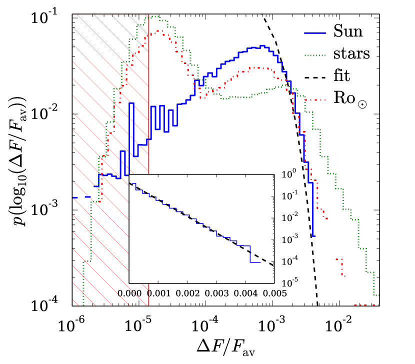
Figure 4.— Probability distribution function for observing a brightness variation $\Delta F/F_{\rm av}$ at a random time between 1874 May and 2013 July on the Sun (solid, blue line) for the 115,989 stars used in Figure 3 (dotted, green line) and stars with Rossby numbers within $10\%$ of the solar value (dash-dotted, red line). The inset shows the probability distribution $p(\Delta F/F_{\rm av})$ together with the fit. We fit the Sun’s data with the function $0.4\times\exp(-1750\Delta F/F_{\rm av})$ (dashed, black line). The hatched area indicates the detection limit.

3.3. Superflares Related to Starspot Coverage

Flares originate at the areas above starspots (Sammis et al., 2000) where magnetic field lines reconnect and give rise to particle acceleration. Since we use the relative flux variation as a proxy for the area covered by starspots, we expect more frequent superflares as $\Delta F/F_{\rm av}$ increases. For the average superflare occurrence frequency, we determine an approximate power law of $\nu_{\rm tot}\tau\propto\Delta F/F_{\rm av}$ (Figure 5). Since we expect the flare area to increase with increasing $\Delta F/F_{\rm av}$, we also expect the frequency of flares to increase with the same power.

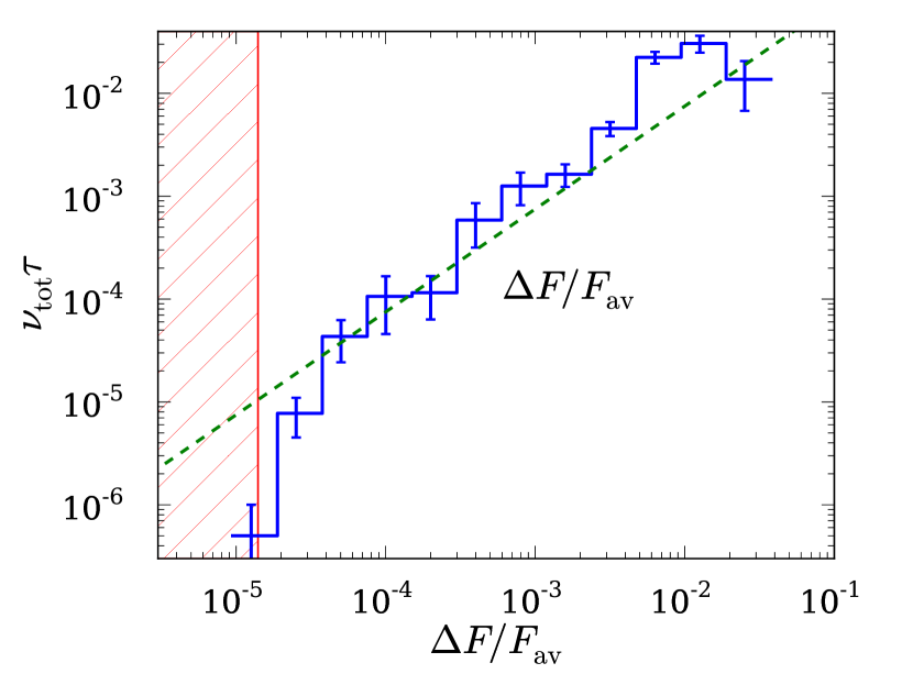
Figure 5.— Average superflare occurrence rate dependent on the relative brightness variation including all the 115,984 stars observed. The hatched area indicates the detection limit.

From Figures 2 and 5, we can conclude that an increase in the inverse Rossby number and/or starspot coverage will lead to an increase in the superflare occurrence rate. Increased brightness variation, however, is a consequence of increased rotation rate, as shown in Figure 3. The question to answer now is whether or not a star with strong brightness variation will show high superflare rates regardless of the Rossby number. To clarify this, we plot the binned average of the superflare occurrence rate $\nu_{\rm tot}\tau$ for all the 115,984 stars as a function of both $\mbox{\rm Ro}^{-1}$ and $\Delta F/F_{\rm av}$ (Figure 6). This clearly shows a dependence of $\nu_{\rm tot}\tau$ on $\Delta F/F_{\rm av}$, while the dependence on $\mbox{\rm Ro}^{-1}$ is comparatively weak for fixed $\Delta F/F_{\rm av}$. As an example, consider the horizontal ridge in Figure 6 through $\Delta F/F_{\rm av}=10^{-2}$, along which the value of $\nu_{\rm tot}\tau$ is nearly the same, regardless of the value of $\mbox{\rm Ro}^{-1}$. Hence, fast rotation leads to high starspot coverage, which increases the chance for superflare eruptions.

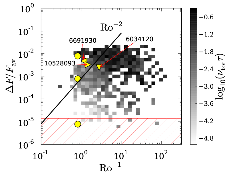
Figure 6.— Binned average for the superflare occurrence rate $\nu_{\rm tot}\tau$ dependent on the inverse Rossby number $\mbox{\rm Ro}^{-1}$ and the brightness variation $\Delta F/F_{\rm av}$. The yellow triangles and circles indicate the same stars, respectively, and our Sun, as described in Figure 3. The hatched area indicates the detection limit. As there is only a weak dependence of the superflare rate on the inverse Rossby number for constant $\Delta F/F_{\rm av}$, we can safely conclude that we can observe superflares due to the appearance of starspots. Those, in turn, are a product of fast rotation.

4. Starspot Modeling and Brightness Variation

As alluded to earlier, we need to clarify to what extent the brightness variation $\Delta F/F_{\rm av}$ can be used as proxy for starspot coverage. Since we cannot resolve the stars, we perform model calculations for the brightness variation of stars covered with spots. For each realization of the spot distribution, the flux variation during one rotation is determined as a function of the star’s inclination angle. From that data, we determine the spread of the starspot coverage for given ranges of $\Delta F/F_{\rm av}$.

A similar analysis was performed by Kovari & Bartus (1997), who reconstructed light curves from a synthetic measurement of an observed star with 10 spots by using model stars with 2 spots. To find the parameters of the two-spot model, they applied a minimization technique which showed large uncertainties and a strong dependence on the initial guess. Since those fitting curves could approximate the synthetic light curve very well, it could be concluded that there are strong ambiguities in the reconstruction of such light curves. Using a two-spot model, Notsu et al. (2013) reconstructed observed light curves for stars at given inclinations. On this basis, they concluded that the brightness variation approximates the spot coverage well. They did not, however, determine the ambiguity which arises from applying different inclination angles and more than two spots. In our starspot model, the aim is to make as few assumptions as possible and to determine quantitatively the uncertainties.

4.1. Model Stars

We create a starspot map by randomly choosing the spot center on the stellar surface in azimuth $\phi$ and latitude $\theta$, with the limits $0\leq\phi<2\pi$ and $-\pi/2<\theta<\pi/2$. For $\phi$ and $\theta$, random and uniformly distributed within their limits, a higher density of spots is obtained near the poles. This is automatically mitigated by choosing the spot size such that $A_{\rm spot}\propto\cos\theta$. Hence, the probability density function of spot coverage is a constant in $\phi$ and $\theta$. We know that for the Sun they appear more frequently close to the equator at about $\pm 30^{\circ}$ latitude. We do not assume any such preferential distribution for our stars. Furthermore, in our model stars, spots may extend over the equator and the poles, thus allowing for a very general spot distribution.

For simplicity, the spots are taken to be segments of linear size $s$ extending from $\phi-s/2$ to $\phi+s/2$ and $\theta-s/2$ to $\theta+s/2$, where $s$ is a random value between $0$ and $\pi/5$, thus covering up to $3\%$ of the star’s surface. With a random number of spots between $0$ and $10$, we can cover up to approximately a third of the surface. Of course, starspots are not square-like, but for our statistical analysis this is a good enough approximation. An example spot coverage is plotted in Figure 7 where the dark areas indicate spots and the white areas are free of spots.

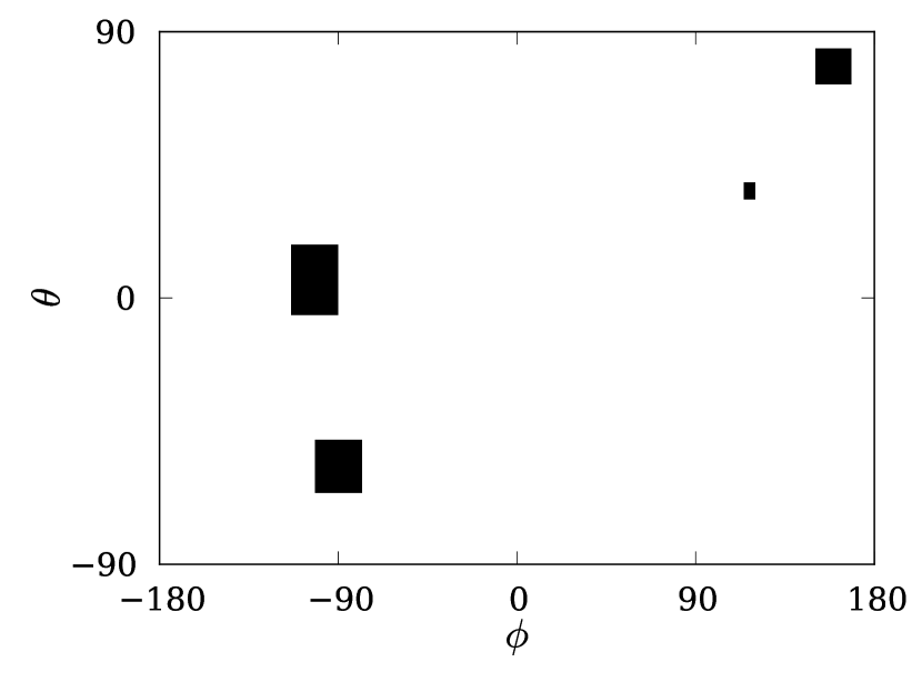
Figure 7.— Starspot map example used in the statistical analysis (equirectangular projection). The dark areas are those covered by spots and the white areas are free of spots.

4.2. Synthetic Observations

From our starspot maps, such as Figure 7, we can extract measurements of the observed brightness as a function of the inclination angle $i$ of the observer to the equatorial plane and the facing meridian $\phi$. The latter is sampled through to simulate the star’s rotation, which then gives rise to a flux curve from which we extract $F_{\rm av}$ and $\Delta F$. The total flux of the observed disk depends on the disk coverage with spots and is simply the integral of the flux over the disk. For the spot temperature, we use a solar value of $T_{\rm s}=4000\,{\rm K}$ and a photospheric temperature of $T_{\rm p}=5800\,{\rm K}$. The emitted flux is proportional to $T^{4}$. Since no information is available on the radial density and temperature distribution of the stars, we neglect limb darkening effects. Furthermore, we do not consider small-scale bright regions such as plages.

We plot the observed flux dependent on $\phi$ and $i$ and obtain the brightness map in Figure 8 for the previous example, where $F(\phi,i)$ is the observed flux at a given inclination angle and facing meridian, i.e., the rotation phase. Comparing with Figure 7, we can readily confirm the validity of the synthetic observations.

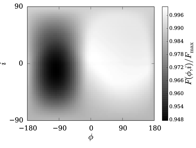
Figure 8.— Observed brightness of a star with spot distribution shown in Figure 7 dependent on the facing meridian $\phi$ and inclination angle $i$ (equirectangular projection).

4.3. Statistical Spread

In order to obtain good statistics, we create 3771 realizations of starspot distributions, each of which leads to a different starspot coverage $A_{\rm spot}$. Should the observed brightness variation be weakly dependent on the particular realization or the star’s inclination, we may conclude that $\Delta F/F_{\rm av}$ is a good proxy for starspot coverage.

In Figure 9 we plot a map of the fractional spot coverage for all inclinations and realizations as a function of the brightness variation. A general trend can readily be seen. As the brightness variation increases, the expected spot coverage also increases. To determine the statistical significance, we bin the data for various intervals of $\Delta F/F_{\rm av}$ and determine the mean for $A_{\rm spot}$. Since high inclination angles are statistically less likely than face-on observations, we need to weigh the significance of the data according to the weight $\omega=\cos i$.

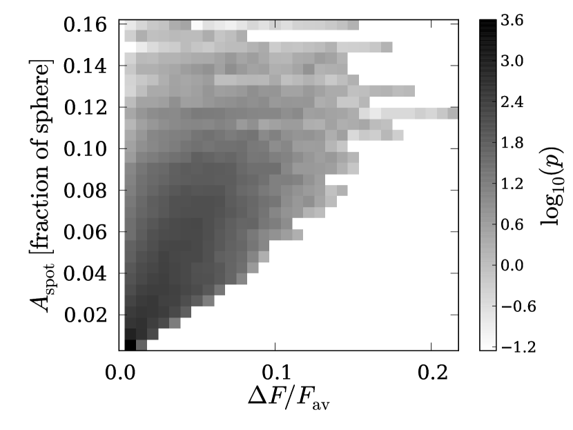
Figure 9.— Starspot coverage map from synthetic measurements for 3771 different realizations of starspot coverage for various inclination angles dependent on the brightness variation.

The mean follows a general trend such that $A_{\rm spot}\propto\Delta F/F_{\rm av}$ (Figure 10). Of greater significance here is the standard deviation $\sigma$, which shows the spread of the data for the various inclination angles and realizations. We find that $\sigma$ is comparable to the slope of the general trend. Together with the apparent trend, we conclude that $\Delta F/F_{\rm av}$ is a useful proxy for $A_{\rm spot}$.

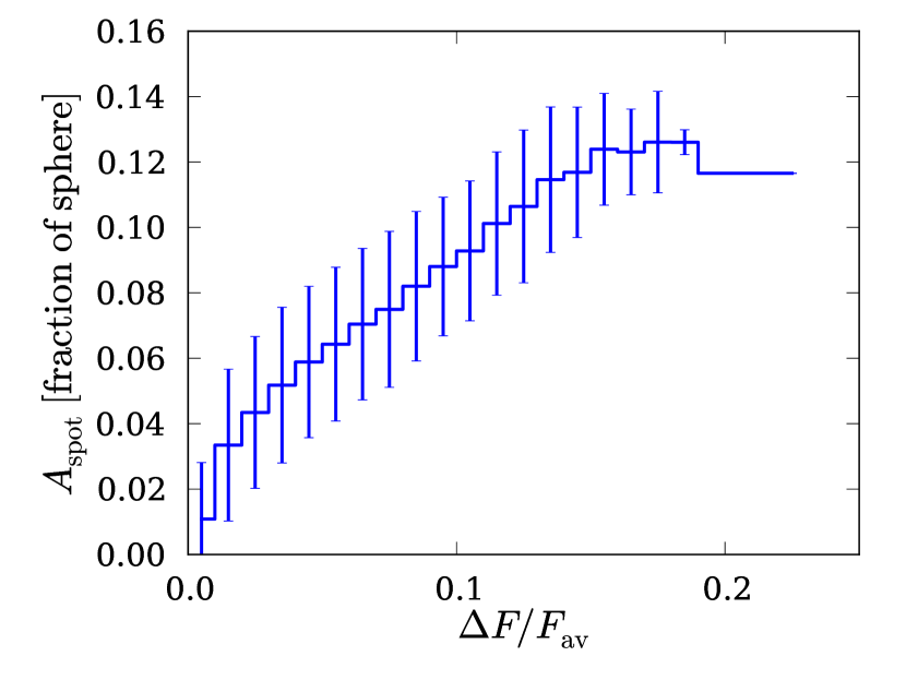
Figure 10.— Binned averages for the starspot coverage for intervals of the observed brightness variation, together with the standard deviation. A general trend is observed where $A_{\rm spot}$ appears to be proportional to $\Delta F/F_{\rm av}$.

5. Flare Energy

5.1. Rotation Rate Affecting Flare Energy

With increasing values of $\mbox{\rm Ro}^{-1}$, we first observe an increase and then a decrease in $\nu_{\rm tot}\tau$ (Figure 2). We test whether or not the individual flare energy depends on $\mbox{\rm Ro}^{-1}$ using a data set containing 6830 flares of 795 stars. We know the Rossby number and brightness variation for 753 of those stars for a total of 6568 flare events. In Figure 11, we plot the relative flare population for intervals of $\mbox{\rm Ro}^{-1}$ and flare energy $E$, and overplot a 1D average. Moving from slow to fast rotators, the average flare energy clearly systematically increases. We can also identify a power law with an exponent of $1/2$. However, the statistical significance is poor.

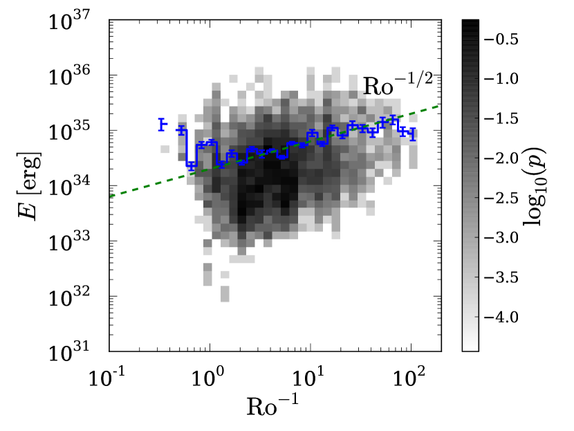
Figure 11.— Binned average for the flare energy in given intervals of $\mbox{\rm Ro}^{-1}$ (1D histogram) together with a fit. The color mapping shows the relative population $p$ of flares within intervals of $\mbox{\rm Ro}^{-1}$ and flare energy. From the fit, it becomes clear that more energetic flares can be expected from faster rotating stars.

5.2. Flare Energy Distribution

Maehara et al. (2012) and Shibayama et al. (2013) determined a power-law behavior for the dependence of flare frequency on flare energy. The dependence was determined to be proportional to $E^{-2.3}$ with an error of $\pm 0.3$ for the slope. By using a data set containing 6830 flares from 795 stars, we determine the total number of flares within a given energy range and reproduce their power-law behavior. From our analysis, we find $n_{\rm flares}(E_{\rm flare})\times E_{\rm flare}^{-1}\propto E_{\rm flare}^{-1.8}$, which is comparable to previous findings (Figure 12). We also check whether or not there is a different behavior for different ranges of the Rossby number for $\mbox{\rm Ro}^{-1}>7$, $7\geq\mbox{\rm Ro}^{-1}>2.5$, and $\mbox{\rm Ro}^{-1}\leq 2.5$, but we find no significant deviation.

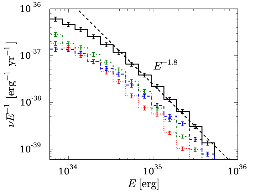
Figure 12.— Frequency distribution for the flare energy including all superflaring stars (solid back line), stars with $\mbox{\rm Ro}^{-1}>7$ (blue dashed line), with $7\geq\mbox{\rm Ro}^{-1}>2.5$ (green dash-dotted line), and $\mbox{\rm Ro}^{-1}\leq 2.5$ (red dotted line).

6. Interpretation and Modeling

The above results show that while stellar activity is correlated with $\mbox{\rm Ro}^{-1}$, flare energy is only poorly correlated and shows significant scatter in this relation; see Figure 11. Whether or not this agrees quantitatively with the dynamo predictions can be assessed through numerical simulations.

In turbulent dynamos, magnetic energy is distributed over a broad range of scales. The magnetic field seen in the solar cycle corresponds only to the lowest wavenumbers of the magnetic energy spectrum. However, the remaining part of the spectrum is quite independent of the cycle and, presumably, also of the occurrence of grand minima. Furthermore, we recall that evidence from ¹⁰Be isotope measurements in the Greenland ice cores (Beer et al., 1998) revealed cyclic activity even during the Maunder minimum. Therefore, even cycles themselves are independent of the overall activity state of the system, be it in a grand minimum or grand maximum. However, because the magnetic field remains highly turbulent, involving all scales, we must expect a certain level of fluctuations, which becomes more intense toward smaller scales.

In hydromagnetic turbulence, magnetic dissipation is proportional to the square of the current density, which is characteristic of the smallest scales in the spectrum. To further illustrate this, let us now consider a simple turbulent dynamo exhibiting cyclic variability. Crucial ingredients of such a dynamo are shear and helical turbulence. This can easily be represented in a simulation of helically forced turbulence with linear shear and shearing-periodic boundary conditions. Such models have been studied extensively by Käpylä & Brandenburg (2009) for different values of the scale separation ratio $k_{\rm f}/k_{1}$, where $k_{\rm f}$ is the forcing wavenumber and $k_{1}$ is the lowest wavenumber that fits into the Cartesian domain of size $L^{3}$, so $k_{1}=2\pi/L$. Applications to long-term variability have been studied by Brandenburg & Guerrero (2012) for small values of $k_{\rm f}/k_{1}$ of 1.5 and 2.2, and different shear parameters, $\mbox{\rm Sh}=S/u_{\rm rms}k_{\rm f}$, where $S$ is the shear rate characterizing the strength of the linear shear flow $\overline{\mbox{\boldmath$U$}}{}=(0,Sx,0)$ for a given rms velocity $u_{\rm rms}$ of the turbulence. Applied to stellar differential rotation, the $y$ direction corresponds to the toroidal direction and the $x$ direction to radius, so that the $z$ direction corresponds to the latitude (i.e., negative colatitude). We adopt negative values of $S$, which corresponds to the negative radial shear in the near-surface shear layer. In the solar dynamo, this layer may be important in “shaping” the dynamo wave toward the equator (Brandenburg, 2005; Kosovichev et al., 2013).

In the following, we consider the model of Brandenburg & Guerrero (2012) for $k_{\rm f}/k_{1}=2.2$ and five values of Sh. In particular, we study in detail the statistics of local magnetic dissipation for such a model; see Figure 13 where we compare the local evolution of the toroidal magnetic field $B_{y}$ (which shows cyclic behavior) with that of the local magnetic dissipation rate, $\epsilon\propto\mbox{\boldmath$J$}{}^{2}$ (which shows no clear cycles). Here, $\mbox{\boldmath$J$}{}=\mbox{\boldmath$\nabla$}{}\times\bm{B}/\mu_{0}$ is the current density, $\bm{B}$ is the magnetic field, and $\mu_{0}$ is the vacuum permeability. Note that in the present model where the magnetic Reynolds number is only about 60, the maximum magnetic dissipation is more than 20 times its average. In turbulence theory, the local dissipation statistics is known to obey a log-Poisson distribution for low local dissipation (Dubrulle, 1994), but it is likely to show power-law behavior for high local dissipation (Gledzer et al., 1996). Our present results are roughly compatible with this; see Figure 13, which shows $p(\ln\epsilon)\sim\epsilon^{-2}$.

Figure 13.— Upper panel: time dependence of the toroidal magnetic field $B_{y}$, normalized by the equipartition field strength $B_{\rm eq}$ (dotted line) compared with its temporally smoothed evolution (solid line) for a model with $k_{\rm f}/k_{1}=2.2$, $\mbox{\rm Sh}=-2.3$, and $D=27$. Middle panel: local energy dissipation $\epsilon$ normalized by its averaged value $\overline{\epsilon}$. Lower panel: probability density function of $\epsilon/\overline{\epsilon}$. The dashed line indicates a $p\propto\epsilon^{-2}$ scaling.

To compare the resulting statistics for energy dissipation in the model with the statistics of the flare energies of stars shown in Figure 11, we now consider models for different shear parameters Sh. The strength of the resulting large-scale dynamo is characterized by the dynamo number $D$. For $\alpha$–shear dynamos, $D$ is given by the product of two dynamo numbers, $D=C_{\alpha}C_{S}$, where $C_{\alpha}=\alpha/\eta_{\it t}k_{1}$ measures the relative strength of the kinetic helicity, and $C_{S}=S/\eta_{\it t}k_{1}^{2}$ measures the strength of the shear relative to turbulent diffusive effects characterized by the turbulent magnetic diffusivity, $\eta_{\it t}\approx\tau u_{\rm rms}^{2}/3$, where $\tau$ is the correlation time. Estimating the $\alpha$ effect as $\alpha=-\tau\overline{\mbox{\boldmath$\omega$}{}\cdot\mbox{\boldmath$u$}{}}/3$ (Moffatt, 1978), where $\overline{\mbox{\boldmath$\omega$}{}\cdot\mbox{\boldmath$u$}{}}$ is the kinetic helicity with $\mbox{\boldmath$\omega$}{}=\mbox{\boldmath$\nabla$}{}\times\mbox{\boldmath$u$}{}$ being the vorticity of the flow $u$, and estimating $\overline{\mbox{\boldmath$\omega$}{}\cdot\mbox{\boldmath$u$}{}}\approx k_{\rm f}u_{\rm rms}^{2}$ for fully helical turbulence (Candelaresi & Brandenburg, 2013), we find $C_{\alpha}\approx-k_{\rm f}/k_{1}$. Here, the minus sign in the expression for $\alpha$ is due to the fact that $\alpha$ is a negative multiple of the kinetic helicity and that the helicity of the turbulent forcing is positive. For the second dynamo number, we similarly estimate $C_{S}=3\,\mbox{\rm Sh}\,(k_{\rm f}/k_{1})^{2}$ (Brandenburg & Guerrero, 2012). For the model presented in Figure 13, we have $C_{S}\approx-12$. Since $C_{\alpha}<0$, we have $D>0$, which yields dynamo waves traveling in the positive $z$ direction, i.e., toward the equator. Since $C_{\alpha}=\alpha/\eta_{\it t}k_{1}\approx-2.2$, we have $D\approx 27$, which is nearly 14 times larger than the critical value $D_{\rm crit}=2$ for the onset of $\alpha$–shear dynamos (Brandenburg & Subramanian, 2005).

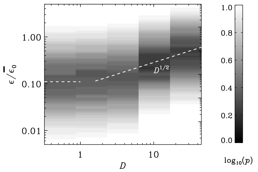
Figure 14.— Probability density function of $\ln(\epsilon/\overline{\epsilon}_{0})$ for five bins of the dynamo number $D$.

In Figure 14, we show the probability density function of the normalized dissipation energy $\ln(\epsilon/\overline{\epsilon}_{0})$ and dynamo number, $D$, where $\overline{\epsilon}_{0}$ is the average kinetic energy input to the dynamo. For $D<D_{\rm crit}$, the dynamo is just a small-scale dynamo, where the median of the dissipation energy is independent of $D$. For larger values of $D$, the median shows a mild increase proportional to $D^{1/2}$, which is reminiscent of the increase of the median of flare energies seen in Figure 11. However, it is not clear how $D$ is related to $\mbox{\rm Ro}^{-1}$, but if they were proportional to each other, then the two graphs would indeed be in quantitative agreement with each other. Furthermore, there is considerable scatter by about one dex, and it might be even stronger for the flare energies seen in Figure 11, where for a given value of $\mbox{\rm Ro}^{-1}$ there can be significant variation.

7. Conclusions

In this paper, we have searched for conditions under which flares with total energies above $5\times 10^{34}{\rm erg}$ occur. We have used data from an extended superflare catalog which had been derived from Kepler data (Maehara et al., 2012). The stars are G-, K- and M-type stars. Of those, only two are binary systems (Matijevič et al., 2012). There is no evidence for “hot Jupiters” orbiting the stars, which makes our findings applicable to the Sun. Given the similarity of the systems, we confirm the earlier findings of Maehara et al. (2012), Shibata et al. (2013), and Shibayama et al. (2013) that there is no need for any external influence, which could affect the magnetic field in the corona, as proposed by Rubenstein & Schaefer (2000).

The two important quantities we found were the effective temperature and the inverse Rossby number, which is a non-dimensional measure of the rotation rate. Dynamo activity is known to decrease with the star’s effective temperature (Kitchatinov & Olemskoy, 2011) which then leads to less frequent and less energetic flares. We observe such a negative dependence for the monitored Kepler stars (Figure 1). From standard dynamo theory, we known that dynamo activity increases with the rotation frequency (e.g., Karak et al., 2014). In Figure 3 (upper panel), we find this behavior for the observed stars where we take the relative flux variation as a proxy for the starspot coverage and magnetic activity.

Statistics from superflaring stars can be deceiving, as we observe two very different results for the superflare occurrence rate dependent on the Rossby number, based on whether or not non-flaring stars are taken into account. Using only superflare stars leads to no significant dependence of the occurrence rate on the rotation rate (Figure 2). This is counterintuitive, since increased rotation should enhance the dynamo. By including all of the observed stars, the average occurrence rate changes due to the number of non-superflaring stars within that bin (Figure 2). That way we obtain two power laws for $\nu_{\rm tot}\tau$ with the powers $-2$ for $\mbox{\rm Ro}^{-1}\lesssim 10$ and $1$ for $\mbox{\rm Ro}^{-1}\gtrsim 10$. This finding is in agreement with Shibayama et al. (2013), who found higher superflare rates for fast rotating stars.

Observational bias arising from random angles between the observer–star axis and its rotation axis is a considerable effect. From the synthetic light curve measurements for our model stars, we see a general trend as well as a significant spread (Figure 10). We conclude that the inference of spot coverage from brightness variation is valid, although it contains some uncertainties.

Flare energies are strongly connected with the rotation rate (Figure 11). This is expected from dynamo theory, as the increase in magnetic energy is positively affected by the rotation rate. The increased dynamo action leads to a higher coverage of spots (Figure 3), and possibly to a higher number of large spots. Those large spots can store larger amounts of magnetic energy which then leads to more energetic flares (Figure 11, color mapping).

Our simulations of a standard dynamo with helically forced turbulence clearly show a characteristic dependence for the Ohmic dissipation rate (Figure 13). This $E^{-2}$ dependence should be compared to $E^{-2.3}$, found by Maehara et al. (2012) and Figure 12. This shows that dissipation follows a power-law behavior. Since the flares originated from such dissipations, this explains the power-law behavior for the flare energy. Exponential tails in the distribution of energy dissipation imply that there is a considerable chance that an extreme dissipation event or superflare could occur in a system whose average activity level is comparatively low.

References

- Barnes et al. (2005) Barnes, J. R., Collier Cameron, A., Donati, J.-F., James, D. J., Marsden, S. C., & Petit, P. 2005, MNRAS, 357, L1
- Beer et al. (1998) Beer, J., Tobias, S., & Weiss, N. 1998, SoPh, 181, 237
- Brandenburg (2005) Brandenburg, A. 2005, ApJ, 625, 539
- Brandenburg & Guerrero (2012) Brandenburg, A., & Guerrero, G. 2012, in IAU Symposium, Vol. 286, Comparative Magnetic Minima: Characterizing Quiet Times in the Sun and Stars, ed. C. H. Mandrini & D. F. Webb (Cambridge University Press), 37
- Brandenburg et al. (2012) Brandenburg, A., Sokoloff, D., & Subramanian, K. 2012, SSRv, 169, 123
- Brandenburg & Subramanian (2005) Brandenburg, A., & Subramanian, K. 2005, PhR, 417, 1
- Candelaresi & Brandenburg (2013) Candelaresi, S., & Brandenburg, A. 2013, PhRvE, 87, 043104
- Carrington (1859) Carrington, R. C. 1859, MNRAS, 20, 13
- Choudhuri et al. (1995) Choudhuri, A. R., Schüssler, M., & Dikpati, M. 1995, A&A, 303, L29
- Dikpati & Charbonneau (1999) Dikpati, M., & Charbonneau, P. 1999, ApJ, 518, 508
- Dubrulle (1994) Dubrulle, B. 1994, PhRvL, 73, 959
- Fröhlich & Lean (1998) Fröhlich, C., & Lean, J. 1998, GeoRL, 25, 4377
- Gledzer et al. (1996) Gledzer, E., Villermaux, E., Kahalerras, H., & Gagne, Y. 1996, PhFl, 8, 3367
- Hodgson (1859) Hodgson, R. 1859, MNRAS, 20, 15
- Käpylä & Brandenburg (2009) Käpylä, P. J., & Brandenburg, A. 2009, ApJ, 699, 1059
- Karak et al. (2014) Karak, B. B., Kitchatinov, L. L., & Choudhuri, A. R. 2014, ApJ, 791, 59
- Kitchatinov & Olemskoy (2011) Kitchatinov, L. L., & Olemskoy, S. V. 2011, MNRAS, 411, 1059
- Koch et al. (2010) Koch, D. G., et al. 2010, ApJL, 713, L79
- Kosovichev et al. (2013) Kosovichev, A. G., Pipin, V. V., & Zhao, J. 2013, in ASP Conf. Ser., Vol. 479, Progress in Physics of the Sun and Stars, ed. H. Shibahashi & A. E. Lynas-Gray (San Francisco, CA: ASP), 395
- Kovari & Bartus (1997) Kovari, Z., & Bartus, J. 1997, A&A, 323, 801
- Maehara et al. (2012) Maehara, H., et al. 2012, Natur, 485, 478
- Malanushenko et al. (2014) Malanushenko, A., Schrijver, C. J., DeRosa, M. L., & Wheatland, M. S. 2014, ApJ, 783, 102
- Matijevič et al. (2012) Matijevič, G., Prša, A., Orosz, J. A., Welsh, W. F., Bloemen, S., & Barclay, T. 2012, AJ, 143, 123
- Moffatt (1978) Moffatt, H. K. 1978, Magnetic Field Generation in Electrically Conducting Fluids (Cambridge: Cambridge Univ. Press)
- Nandy & Choudhuri (2002) Nandy, D., & Choudhuri, A. R. 2002, Sci, 296, 1671
- Nogami et al. (2014) Nogami, D., Notsu, Y., Honda, S., Maehara, H., Notsu, S., Shibayama, T., & Shibata, K. 2014, PASJ, 66, L4
- Notsu et al. (2013) Notsu, Y., et al. 2013, ApJ, 771, 127
- Noyes et al. (1984) Noyes, R. W., Hartmann, L. W., Baliunas, S. L., Duncan, D. K., & Vaughan, A. H. 1984, ApJ, 279, 763
- Pallavicini et al. (1981) Pallavicini, R., Golub, L., Rosner, R., Vaiana, G. S., Ayres, T., & Linsky, J. L. 1981, ApJ, 248, 279
- Pizzolato et al. (2003) Pizzolato, N., Maggio, A., Micela, G., Sciortino, S., & Ventura, P. 2003, A&A, 397, 147
- Pouquet et al. (1976) Pouquet, A., Frisch, U., & Léorat, J. 1976, JFM, 77, 321
- Reinhold et al. (2013) Reinhold, T., Reiners, A., & Basri, G. 2013, A&A, 560, A4
- Rubenstein & Schaefer (2000) Rubenstein, E. P., & Schaefer, B. E. 2000, ApJ, 529, 1031
- Sammis et al. (2000) Sammis, I., Tang, F., & Zirin, H. 2000, ApJ, 540, 583
- Schaefer et al. (2000) Schaefer, B. E., King, J. R., & Deliyannis, C. P. 2000, ApJ, 529, 1026
- Schrijver (2009) Schrijver, C. J. 2009, AdSpR, 43, 739
- Shibata et al. (2013) Shibata, K., et al. 2013, PASJ, 65, 49
- Shibayama et al. (2013) Shibayama, T., et al. 2013, ApJS, 209, 5
- Steenbeck et al. (1966) Steenbeck, M., Krause, F., & Rädler, K.-H. 1966, ZNatA, 21, 369
- Su et al. (2013) Su, Y., Veronig, A. M., Holman, G. D., Dennis, B. R., Wang, T., Temmer, M., & Gan, W. 2013, NatPh, 9, 489
- Veltri et al. (2005) Veltri, P., Nigro, G., Malara, F., Carbone, V., & Mangeney, A. 2005, NPGeo, 12, 245
- Vilhu (1984) Vilhu, O. 1984, A&A, 133, 117
- Walter (1982) Walter, F. M. 1982, ApJ, 253, 745
- Willson et al. (1981) Willson, R. C., Gulkis, S., Janssen, M., Hudson, H. S., & Chapman, G. A. 1981, Sci, 211, 700
- Willson & Hudson (1981) Willson, R. C., & Hudson, H. S. 1981, ApJL, 244, L185
- Wright et al. (2011) Wright, N. J., Drake, J. J., Mamajek, E. E., & Henry, G. W. 2011, ApJ, 743, 48