A Flavor Kit for BSM models
Abstract
We present a new kit for the study of flavor observables in models beyond the standard model. The setup is based on the public codes SARAH and SPheno and allows for an easy implementation of new observables. The Wilson coefficients of the corresponding operators in the effective lagrangian are computed by SPheno modules written by SARAH. New operators can also be added by the user in a modular way. For this purpose a handy Mathematica package called PreSARAH has been developed. This uses FeynArts and FormCalc to derive the generic form factors at tree- and 1-loop levels and to generate the necessary input files for SARAH. This framework has been used to implement BR(), BR(), CR(), BR(), BR(), BR(), BR(), BR(), BR(), BR(), BR(), BR(), , , , BR(), BR(), BR() and BR() in SARAH. Predictions for these observables can now be obtained in a wide range of SUSY and non-SUSY models. Finally, the user can use the same approach to easily compute additional observables.
1 Introduction
With the exploration of the terascale, particle physics has entered a new era. On the one hand, the discovery of a Higgs boson at the LHC Aad:2012tfa ; Chatrchyan:2012ufa seemingly completed the Standard Model (SM) of particle physics, even though there is still quite some room for deviations from the SM predictions. The observed mass of about 125 GeV in combination with a top quark mass of 173.34 GeV ATLAS:2014wva implies within the SM that we potentially live in a meta-stable vacuum Buttazzo:2013uya . This, together with other observations, like the dark matter relic density or the unification of gauge forces, indicates that there is physics beyond the SM (BSM). Although no sign of new physics has been found so far at the LHC, colliders are not the only places where one can search for new physics. Low energy experiments focused on flavor observables can also play a major role in this regard, since new particles leave their traces via quantum effects in flavor violating processes such as , or . In the last few years there has been a tremendous progress in this field, both on the experimental as well as on the theoretical side. In particular, observables from the Kaon- and B-meson sectors, rare lepton decays and electric dipole moments have put stringent bounds on new flavor mixing parameters and/or additional phases in models beyond the SM.
There are several public tools on the market which predict the rates of several flavor observables: superiso Mahmoudi:2007vz ; Mahmoudi:2008tp ; Mahmoudi:2009zz , SUSY_Flavor Rosiek:2010ug ; Crivellin:2012jv , NMSSM-Tools Ellwanger:2006rn , MicrOmegas Belanger:2001fz ; Belanger:2004yn ; Belanger:2006is ; Belanger:2008sj ; Belanger:2013oya , SuperBSG Degrassi:2007kj , SupeLFV Murakami:2013rca , SuseFlav Chowdhury:2011zr , IsaJet with IsaTools Paige:2003mg ; Baer:2003xc ; Baer:1999sp ; Paige:1998xm ; Paige:1998ux ; Baer:1993ae or SPheno Porod:2003um ; Porod:2011nf . However, all of these codes have in common that they are only valid in the Two-Higgs-doublet model or in the MSSM or simple extensions of it (NMSSM, bilinear R-parity violation). In addition, none of these tools can be easily extended by the user to calculate additional observables. This has made flavor studies beyond the SM a cumbersome task. The situation has changed with the development of SARAH Staub:2008uz ; Staub:2009bi ; Staub:2010jh ; Staub:2012pb ; Staub:2013tta . This Mathematica package can be used to generate modules for SPheno, which then can calculate flavor observables at the 1-loop level in a wide range of supersymmetric and non-supersymmetric models Dreiner:2012mx ; Dreiner:2012dh ; Dreiner:2013jta . However, so far all the information about the underlying Wilson coefficients111Sometimes the Wilson coefficients are also referred to as form factors. We will nevertheless stick to the name Wilson coefficients in the following, also for lepton flavor violating processes. for the operators triggering the flavor violation as well as the calculation of the flavor observables had been hardcoded in SARAH. Therefore, it was also very difficult for the user to extend the list of calculated observables. The implementation of new operators was even more difficult.
We present a new kit for the study of flavor observables beyond the standard model. In contrast to previous flavor codes, FlavorKit is not restricted to a single model, but can be used to obtain predictions for flavor observables in a wide range of models (SUSY and non-SUSY). FlavorKit can be used in two different ways. The basic usage of FlavorKit allows for the computation of a large number of lepton and quark flavor observables, using generic analytical expressions for the Wilson coefficients of the relevant operators. The setup is based on the public codes SARAH and SPheno, and thus allows for the analytical and numerical computation of the observables in the model defined by the user. If necessary, the user can also go beyond the basic usage and define his own operators and/or observables. For this purpose, a Mathematica package called PreSARAH has been developed. This tool uses FeynArts/FormCalc Hahn:1998yk ; Hahn:2000kx ; Hahn:2000jm ; Hahn:2004rf ; Hahn:2005vh ; Nejad:2013ina to compute generic expressions for the required Wilson coefficients at the tree- and 1-loop levels. Similarly, the user can easily implement new observables. With all these tools properly combined, the user can obtain analytical and numerical results for the observables of his interest in the model of his choice. To calculate new flavor observables with SPheno for a given model the user only needs the definition of the operators and the corresponding expressions for the observables as well as the model file for SARAH. All necessary calculations are done automatically. We have used this setup to implement BR(), BR(), CR(), BR(), BR(), BR(), BR(), BR(), BR(), BR(), BR(), BR(), , , , BR(), BR(), BR() and BR() in SARAH.
This manual is structured as follows: in the next section we give a brief introduction into the calculation of flavor observables focusing on the main steps that one has to follow. Then we present FlavorKit, our setup to combine FeynArts/FormCalc, SPheno and SARAH in Section 3. In Section 4 we explain how new observables can be added and in Section 5 how the list of operators can be extended by the user. A comparison between FlavorKit and the other public codes is presented in Section 6 taking the MSSM as an example before we conclude in Section 7. The appendix contains information about the existing operators and how they have been combined to compute the different flavor observables.
2 General strategy: calculation of flavor observables in a nutshell
Once we have chosen a BSM model 222The current version of FlavorKit can only handle renormalizable operators at this stage of the computation., our general strategy for the computation of a flavor observable follows these steps:
-
•
Step 1: We first consider an effective Lagrangian that includes the operators relevant for the flavor observable of our interest,
(1) This Lagrangian consists of a list of (usually) higher-dimensional operators . The Wilson coefficients can be induced either at tree or at higher loop levels and include both the SM and the BSM contributions (). They encode the physics of our model.
-
•
Step 2: The Wilson coefficients are computed diagrammatically, taking into account all possible tree-level and 1-loop topologies leading to the operators 333In principle, one can go beyond the 1-loop level, although in our case we will restrict our computation to the addition of a few NLO corrections..
-
•
Step 3: The results for the Wilson coefficients are plugged in a general expression for the observable and a final result is obtained.
The user has to make a choice in step 1. The list of operators in the effective Lagrangian can be restricted to the most relevant ones or include additional operators beyond the leading contribution, depending on the required level of precision. Usually, the complete set of renormalizable operators contributing to the observable of interest is considered, although in some well motivated cases one may decide to concentrate on a smaller subset of operators. This freedom is not present in step 2. Once the list of operators has been arranged, the computation of the corresponding coefficients follows from the consideration of all topologies (penguin diagrams, box diagrams, …) leading to the operators. This is the most complicated and model dependent step, since it demands a full knowledge of all masses and vertices in the model under study. Furthermore, it may be necessary to compute the coefficients at an energy scale and then obtain, by means of their renormalization group running, their values at a different scale. Finally, step 3 is usually quite straightforward since, like step 1, is model independent. In fact, the literature contains general expressions for most flavor observables, thus facilitating the final step. However, one should be aware that the formulas given in the literature assume that certain operators contribute only sub-dominantly and, thus, omit the corresponding contributions. This is in general justified for the SM but not in a general BSM model. In particular, this is the case for processes involving external neutrinos, which are often assumed to be purely left-handed, making the operators associated to their right-handed components to be neglected.
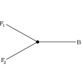
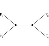
We will exemplify our strategy using a simple example: BR() in the Standard Model extended by right-handed neutrinos and Dirac neutrino masses. The starting point is, as explained above, to choose the relevant operators. In this case, it is well known that only dipole interactions can contribute to to the radiative decay at leading order 444At next to leading order, one would also have to consider operators like , to be combined with a dipole interaction.. Therefore, the relevant operators are contained in the dipole interaction Lagrangian. This is in general given by
| (2) |
Here is the electric charge, the photon momentum, are the usual chirality projectors and denote the lepton flavors. This concludes step 1.
The information about the underlying model is encoded in the coefficients . In the next step, these coefficients have to be calculated by summing up all Feynman diagrams contributing at a given loop level. Expressions for these coefficients for many different models are available in the literature. In the SM only neutrino loops contribute and one finds Ma:1980gm
| (3) | ||||
| (4) |
Here, denote the entries of the Pontecorvo-Maki-Nakagawa-Sakata matrix and and are loop functions. One finds approximately and . Finally, we just need to proceed to the last step, the computation of the observable. After computing the Wilson coefficients it is easy to relate them to BR() by using Hisano:1995cp
| (5) |
This expression holds for all models. With this final step, the computation concludes.
As we have seen, the main task to get a prediction for BR() in a new model is to calculate . However, this demands the knowledge of all masses and vertices involved. Moreover, in most cases a numerical evaluation of the resulting loop integrals is also welcome. Therefore, even for a simple process like , a computation from scratch in a new model can be a hard work. In order to solve this practical problem, we are going to present here a fully automatized way to calculate a wide range of flavor observables for several classes of models.
3 Setup
3.1 FlavorKit: usage and goals
As we have seen, the calculation of flavor observables in a specific model is a very demanding task. A detailed knowledge about the model is required, including
-
1.
expressions for all involved masses and vertices
-
2.
optionally, renormalization group equations to get the running parameters at the considered scale
-
3.
expressions to calculate the operators
-
4.
formulae to obtain the observables from the operators
Nearly all codes devoted to flavor physics have those pieces hardcoded, and they are only valid for a few specific models 555Recently, Peng4BSM@LO Bednyakov:2013tca was made public. This code derives analytical expressions for vector penguins for a model defined in the corresponding FeynArts model file.. The only exception is SPheno, thanks to its extendability with new modules for additional models. These modules are generated by the Mathematica package SARAH and provide all necessary information about the calculation of the (loop corrected) mass spectrum, the vertices and the 2-loop RGEs. These expressions, derived from fundamental principles for any (renormalizable) model, contain all the information required for the computation of flavor observables. In fact, SARAH also provides Fortran code for a set of flavor observables. For this output, generic expressions of the necessary Wilson coefficients have been included. These are matched to the model chosen by the user and related to the observables by the standard formulae available in the literature. However, it was hardly possible for the user to extend the list of observables or operators included in SARAH without a profound knowledge of either the corresponding Mathematica or Fortran code.
We present a new setup to fill this gap in SARAH: FlavorKit. As discussed in Sec. 2, the critical step in the computation of a flavor observable is the derivation of analytical expressions for the Wilson coefficients of the relevant operators. This step, being model dependent, requires information about the model spectrum and interactions. However, generic expressions can be derived, later to be matched to the specific spectrum and interaction Lagrangian of a given model. For this purpose, we have created a new Mathematica package called PreSARAH. This package uses the power of FeynArts and FormCalc to calculate generic 1-loop amplitudes, to extract the coefficients of the demanded operators, to translate them into the syntax needed for SARAH and to write the necessary wrapper code. PreSARAH works for any 4-fermion or 2-fermion-1-boson operators and will be extended in the future to include other kinds of operators. The current version already contains a long list of fully implemented operators (see Appendix B). The results for the Wilson coefficients obtained with PreSARAH are then interpreted by SARAH, which adapts the generic expressions to the specific details of the model chosen by the user and uses snippets of Fortran code to calculate flavor observables from the resulting Wilson coefficients. As for the operators, there is a long list of observables already implemented (see Appendices C.1 and C.2). Finally, SARAH can be used to obtain analytical output in LaTeX format or to create Fortran modules for SPheno, thus making possible numerical studies.
| Lepton flavor | Quark flavor |
|---|---|
| conversion in nuclei | |
| and | |
FlavorKit can be used in two ways:
-
•
Basic usage: This is the approach to be followed by the user who does not need any operator nor observable beyond what is already implemented in FlavorKit. In this case, FlavorKit reduces to the standard SARAH package. The user can use SARAH to obtain analytical results for the flavor observables and, if he wants to make numerical studies, to produce Fortran modules for SPheno. For the list of implemented operators we refer to Appendix B, whereas the list of implemented observables is given in Table 1.
-
•
Advanced usage: This is the approach to be followed by the user who needs an operator or an observable not included in FlavorKit. In case the user is interested in an operator that is not implemented in FlavorKit, he can define his own operators and get analytical results for their coefficients using PreSARAH. Then the output can be passed to SARAH in order to continue with the basic usage. In case the user is interested in an observable that is not implemented in FlavorKit, this can be easily implemented by the addition of a Fortran file, with a few lines of code relating the observable to the operators in FlavorKit (implemented by default or added by the user). The Fortran files just have to be put together with a short steering file into a specific directory located in the main SARAH directory. Then one can continue with the basic usage.

The combination of PreSARAH together with SARAH and SPheno allows for a modular and precise calculation of flavor observables in a wide range of particles physics models. We have summarized the setup in Fig. 1: the user provides as input SARAH model files for his favorite models or takes one of the models which are already implemented in SARAH (see Appendix D for a list of models available in SARAH). New observables are implemented by providing the necessary Fortran code to SARAH while new operators can be either implemented by hand or by using PreSARAH which then calls FeynArts and FormCalc for the calculation of the necessary diagrams. However, most users will not require to implement new operators or observables. In this case, the user can simply use SARAH in the standard way and (1) derive analytical results for the Wilson coefficients and observables, and (2) generate Fortran modules for SPheno in order to run numerical analysis.
3.2 Download and installation
FlavorKit involves several public codes. We proceed to describe how to download and install them.
-
1.
FeynArts/FormCalc
FeynArts and FormCalc can be downloaded fromwww.feynarts.de/
It is also possible to use the script FeynInstall, to be found on the same site, for an automatic installation.
-
2.
SARAH and PreSARAH
SARAH can be downloaded fromsarah.hepforge.org/
No installation or compilation is necessary. Both packages just need to be extracted by using tar.
> tar -xf SARAH-4.2.0
> tar -xf PreSARAH-1.0.0
PreSARAH needs the paths to load FeynArts and FormCalc. These have to be provided by the user in the file PreSARAH.iniThis would work if FeynArts and FormCalc have been installed in the Application directory of the local Mathematica installation. Otherwise, absolute paths should be used, e.g.
1FeynArtsPackage = "/home/$user/$path/FeynArts-3.7/FeynArts.m";2FormCalcPackage = "/home/$user/$path/FormCalc-8.1/FormCalc.m"; -
3.
SPheno
SPheno can be downloaded fromspheno.hepforge.org/
After extracting the package, make is used for the compilation.
> tar -xf SPheno-3.3.0.tar.gz
> cd SPheno-3.3.0
> make
3.3 Basic usage
As explained above, FlavorKit can be used in several ways, depending on the user’s needs and interests. The advanced usage, which involves the introduction of new observables and/or the computation of new operators, is explained in detail in Secs. 4 and 5. Here we focus on the basic usage, which just requires the codes SARAH and SPheno.
SARAH can handle the analytical derivation of all the relevant Wilson coefficients in the model defined by the user. The resulting expressions can be then extracted in LaTeX form or used to generate a SPheno module for numerical evaluation. These are the steps to follow in order to use SARAH:
-
1.
Loading SARAH: after starting Mathematica, SARAH is loaded via
<<SARAH-4.2.0/SARAH.m
or via
<<[$path]/SARAH-4.2.0/SARAH.m
The first choice works if SARAH has been installed in the Application directory of Mathematica. Otherwise, the absolute path ([$path]) to the local SARAH installation must been used. -
2.
Initialize a model: as example for the initialization of a model in SARAH we consider the NMSSM:
Start[“NMSSM”]; -
3.
Obtaining the LaTeX output: the user can get LaTeX output with all the information about the model (including the coefficients for the flavor operators) via
ModelOutput[EWSB];
MakeTeX[]; -
4.
Obtaining the SPheno code: to create the SPheno output the user should run
MakeSPheno[];
Thanks to FlavorKit, SARAH can also write LaTeX files with the analytical expressions for the Wilson coefficients. These are given individually for each Feynman diagram contributing to the coefficients, and saved in the folder
[$SARAH]/Output/[$MODEL]/EWSB/TeX/FlavorKit/
For the 4-fermion operators the results are divided into separated files for tree-level contributions, penguins contributions and box contributions. The corresponding Feynman diagrams are drawn by using FeynMF Ohl:1995kr . To compile all Feynman diagrams at once and to generate the pdf file, a shell script called MakePDF_[$OPERATOR].sh is written as well by SARAH.
In case the user is interested in the numerical evaluation of the flavor observables, a SPheno module must be created as explained above. Once this is done, the resulting Fortran code can be used for the numerical analysis of the model. This can be achieved in the following way:
-
1.
building SPheno: as soon as the SPheno output is finished, open a terminal and enter the root directory of the SPheno installation, and create a new subdirectory, copy the SARAH output to that directory and compile it
> cd [$SPheno]
> mkdir NMSSM
> cp [$SARAH]/Output/NMSSM/EWSB/SPheno/* NMSSM/
> make Model=NMSSM -
2.
Running SPheno: After the compilation, a new binary SPhenoNMSSM is created. This file can be executed providing a standard Les Houches input file (SARAH provides an example file, see the SARAH output folder). Finally, SPheno is executed via
> ./bin/SPhenoNMSSM NMSSM/LesHouches.in.NMSSMThis generates the output file SPheno.spc.NMSSM, which contains the blocks QFVobservables and LFVobservables. In those two blocks, the results for quark and lepton flavor violating observables are given.
Finally, an even easier way to implement new models in SARAH is the butler script provided with the SUSY Toolbox Staub:2011dp
sarah.hepforge.org/Toolbox/
3.4 Limitations
FlavorKit is a tool intended to be as general as possible. For this reason, there are some limitations compared to codes which perform specific calculations in a specific model. Here we list the main limitations of FlavorKit:
-
•
Chiral resummation is not included because of its large model dependence, see e.g. Crivellin:2011jt and references therein.
-
•
Even though we have included some of the higher order corrections for the SM part of some observables in a parametric way, 2- or higher loop corrections, calculated in the context of the SM or the MSSM for specific observables, are not considered, see for instance Buras:1990fn ; Buchalla:1993wq ; Ciuchini:1996sr ; Buras:1999st ; Misiak:2006ab ; Buras:2002tp ; Boughezal:2007ny ; Buras:2012fs .
4 Advanced usage I: Implementation of new observables using existing operators
In order to introduce new observables to the SPheno output of SARAH, the user can add new definitions to the directories
[$SARAH]/FlavorKit/[$Type]/Processes/
[$Type] is either LFV for lepton flavor violating or QFV for quark flavor violating observables. The definition of the new observables consists of two files
-
1.
A steering file with the extension .m
-
2.
A Fortran body with the extension .f90
The steering file contains the following information:
-
•
NameProcess: a string as name for the set of observables.
-
•
NameObservables: names for the individual observables and numbers which are used to identify them later in the SPheno output. The value is a three dimensional list. The first part of each entry has to be a symbol, the second one an integer and the third one a comment to be printed in the SPheno output file ({{name1,number1,comment1},…}).
- •
-
•
Body: The name (as string) of the file which contains the Fortran code to calculate the observables from the operators.
For instance, the corresponding file to calculate reads
The observables will be saved in the variables muEgamma, tauEgamma, tauMuGamma and will show up in the spectrum file written by SPheno in the block FlavorKitLFV as numbers 701 to 703.
The file which contains the body to calculate the observables should be standard Fortran90 code. For our example it reads
Real(dp) is the SPheno internal definition of double precision variables. Similarly one would have to use Complex(dp) for complex double precision variables when necessary.
Besides the operators, the SM parameters given in Table 2 and the hadronic parameters given in Tables 3 and 4 can be used in the calculations. For instance, we used Alpha for and mf_l which contains the poles masses of the leptons as well as GammaMu and GammaTau for the total widths of and leptons.
| Real Variables | |||||
|---|---|---|---|---|---|
| AlphaS_MZ | AlphaS_160 | ||||
| sinW2_MZ | at | sinW2_160 | at | sinW2 | |
| Alpha_MZ | Alpha_160 | Alpha | |||
| MW_MZ | MW_160 | MW | |||
| GammaMu | Width of | GammaTau | Width of | ||
| Real Vectors of length 3 | |||||
| mf_d_160 | mf_d_MZ | mf_d | |||
| mf_u_160 | mf_u_MZ | mf_u | |||
| mf_l_160 | mf_l_MZ | mf_l | |||
| Complex Arrays of dimension | |||||
| CKM_MZ | CKM at | CKM_160 | CKM at | CKM | input |
| Particle | Life time | default [s] | Mass | default [GeV] | PDG number |
|---|---|---|---|---|---|
| tau_pi0 | mass_pi0 | 0.13498 | 111 | ||
| tau_pip | mass_pip | 0.13957 | 211 | ||
| tau_rho0 | mass_rho0 | 0.77549 | 113 | ||
| tau_D0 | mass_D0 | 1.86486 | 421 | ||
| tau_Dp | mass_Dp | 1.86926 | 411 | ||
| tau_DSp | mass_DSp | 1.96849 | 431 | ||
| tau_DSsp | - | mass_DSsp | 2.1123 | 433 | |
| tau_eta | mass_eta | 0.54785 | 221 | ||
| tau_etap | mass_etap | 0.95778 | 331 | ||
| tau_omega | mass_omega | 0.78265 | 223 | ||
| tau_phi | mass_phi | 1.01946 | 333 | ||
| tau_KL0 | mass_KL0 | - | 130 | ||
| tau_KS0 | mass_KS0 | - | 310 | ||
| tau_K0 | - | mass_K0 | 0.49761 | 311 | |
| tau_Kp | mass_Kp | 0.49368 | 321 | ||
| tau_B0d | mass_B0d | 5.27958 | 511 | ||
| tau_B0s | mass_B0s | 5.36677 | 531 | ||
| tau_Bp | mass_Bp | 5.27925 | 521 | ||
| tau_B0c | mass_B0c | 5.3252 | 513 | ||
| tau_Bpc | mass_Bpc | 5.3252 | 523 | ||
| tau_Bcp | mass_Bcp | 6.277 | 541 | ||
| tau_K0c | mass_K0c | 0.8959 | 313 | ||
| tau_Kpc | mass_Kpc | 0.8917 | 323 | ||
| tau_etac | mass_etac | 2.9810 | 441 | ||
| tau_JPsi | mass_JPSi | 3096.92 | 443 | ||
| tau_Ups | mass_Ups | 9.4603 | 553 |
| Decay constant | Variable | default [MeV] | FLHA |
|---|---|---|---|
| f_k_CONST | 176 | FCONST[321,1] | |
| f_Kp_CONST | 156 | FCONST[323,1] | |
| f_pi_CONST | 118 | FCONST[111,1] | |
| f_B0d_CONST | 194 | FCONST[511,1] | |
| f_B0s_CONST | 234 | FCONST[531,1] | |
| f_Bp_CONST | 234 | FCONST[521,1] | |
| f_etap_CONST | 172 | FCONST[231,1] | |
| f_rho_CONST | 220 | FCONST[213,1] | |
| f_Dp_CONST | 256 | FCONST[411,1] | |
| f_Ds_CONST | 248 | FCONST[431,1] |
By extending or changing the file hadronic_parameters.m in the FlavorKit directory, it is possible to add new variables for the mass or life time of mesons. These variables are available globally in the resulting SPheno code. The numerical values for the hadronic parameters can be changed in the Les Houches input file by using the blocks FCONST and FMASS defined in the Flavor Les Houches Accord (FLHA) Mahmoudi:2010iz .
It may happen that the calculation of a specific observable has to be adjusted for each model. This is for instance the case when (1) the calculation requires the knowledge of the number of generations of fields, (2) the mass or decay width of a particle, calculated by SPheno, is needed as input, or (3) a rotation matrix of a specific field enters the analytical expressions for the observable. For these situations, a special syntax has been created. It is possible to start a line with @ in the Fortran file. This line will then be parsed by SARAH, and Mathematica commands, as well as SARAH specific commands, can be used. We made use of this functionality in the implementation of . The lines in hLLp.f90 read
In this implementation we define an integer hLoc that gives the generation index of the SM-like Higgs, to be found among all CP even scalars. In the first line it is checked if more than one scalar Higgs is present. If this is the case, the hLoc is set to the component which has the largest amount of the up-type Higgs, if not, it is just put to 1. Of course, this assumes that the electroweak basis in the Higgs sector is always defined as as is the case for all models delivered with SARAH. In the second and third lines, the variables mh and gamh are set to the mass and total width of the SM-like Higgs, respectively. For this purpose, the SARAH commands SPhenoMass[x] and SPhenoWidth[x] are used. They return the name of the variable for the mass and width in SPheno and it is checked if these variables are arrays or not 666 The user can define in the parameters.m and particles.m file for a given model in SARAH the particles which should be taken to be the CP-even or CP-odd Higgs and the parameter that corresponds to their rotation matrices. This is done by using the Description statements Higgs or Pseudo-Scalar Higgs as well as Scalar-Mixing-Matrix or Pseudo-Scalar-Mixing-Matrix. If the particle or parameter needed to calculate an observable is not present or has not been defined, the observable is skipped in the SPheno output.. For the MSSM, the above lines lead to the following code in the SPheno output:
We give in Table 5 the most important SARAH commands which might be useful in this context.
| getGen[x] | returns the number of generations of a particle x |
|---|---|
| getDim[x] | returns the dimension of a variable x |
| SPhenoMass[x] | returns the name used for the mass of a particle x in the SPheno output |
| SPhenoMassSq[x] | returns the name used for the mass squared of a particle x in the SPheno output |
| SPhenoWidth[x] | returns the name used for the width of a particle x in the SPheno output |
| HiggsMixingMatrix | name of the mixing matrix for the CP even Higgs states in a given model |
| PseudoScalarMixingMatrix | name of the mixing matrix for the CP odd Higgs states in a given model |
Many more examples are given in Appendix C.1, where we have added all input files for the calculations of flavor observables delivered with SARAH.
5 Advanced usage II: Implementation of new operators
The user can also implement new operators and obtain analytical expressions for their Wilson coefficients. In this case, he will need to use PreSARAH which, with the help of FeynArts and FormCalc, provides generic expressions for the coefficients, later to be adapted to specific models with SARAH.
5.1 Introduction
New operators can be implemented by extending the content of the folder
[$SARAH]/FlavorKit/[$Type]/Operators/
In the current version of FlavorKit, 3- and 4-point operators are supported. Each operator is defined by a .m-file. These files contain information about the external particles, the kind of considered diagrams (tree-level, self-energies, penguins, boxes) as well as generic expressions for the coefficients. These expressions, derived from the generic Feynman diagrams contributing to the coefficients, are written in the form of a Mathematica code, which can be used to generate Fortran code.
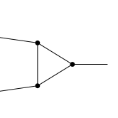
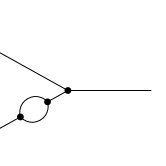
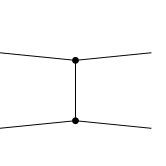
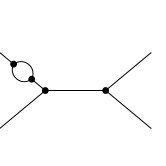
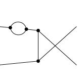
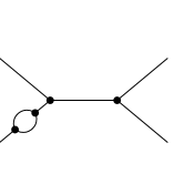
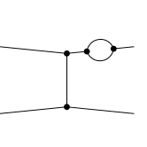
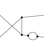
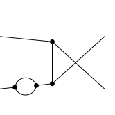
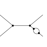
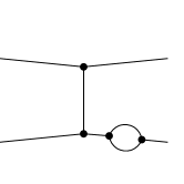
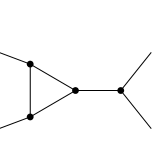
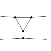
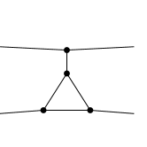
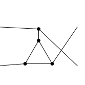
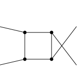
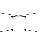
For the automatization of the underlying calculations we have created an additional Mathematica package called PreSARAH, which can be used to create the files for all 4-fermion as well as 2-fermion-1-boson operators. This package creates not only the infrastructure to include the operators in the SPheno output of SARAH but makes also use of FeynArts and FormCalc to calculate the amplitudes and to extract the coefficient of the demanded operators. It takes into account all topologies depicted in Figs. 2 to 6.
 |
||
 |
 |
 |
 |
 |
 |
 |
 |
 |
 |
 |
 |
 |
 |
 |
 |
 |
 |
 |
 |
 |
 |
 |
 |
 |
 |
 |
5.2 Input for PreSARAH
In order to derive the results for the Wilson coefficients, PreSARAH needs an input file with the following information:
-
•
ConsideredProcess: A string which defines the generic type for the process
-
–
“4Fermion”
-
–
“2Fermion1Scalar”
-
–
“2Fermion1Vector”
-
–
-
•
NameProcess: A string to uniquely define the process
-
•
ExternalFields: The external fields. Possible names are ChargedLepton, Neutrino, DownQuark, UpQuark, ScalarHiggs, PseudoScalar, Zboson, Wboson 777 The particles.m file is used to define for each model which particle corresponds to SM states using the Description statement together with Leptons, Neutrinos, Down-Quarks, Up-Quarks, Higgs, Pseudo-Scalar Higgs, Z-Boson, W-Boson. If there is a mixture between the SM particles and other states (like in -parity violating SUSY or in models with additional vector quarks/leptons) the combined state has to be labeled according to the description for the SM state. Notice that in the SM Pseudo-Scalar Higgs is just the neutral Goldstone boson. If an external state is not present in a given model or has not been defined as such in the particles.m file the corresponding Wilson coefficients are not calculated by SPheno.
-
•
FermionOrderExternal: the fermion order to apply the Fierz transformation (see the FormCalc manual for more details)
-
•
NeglectMasses: which external masses can be neglected (a list of integers counting the external fields)
-
•
ColorFlow: defines the color flow in the case of four quark operators. To contract the colors of external fields, ColorDelta is used, i.e ColorFlow = ColorDelta[1,2]*ColorDelta[3,4] assigns .
-
•
AllOperators: a list with the definition of the operators. This is a two dimensional list, where the first entry defines the name of the operator and the second one the Lorentz structure. The operators are expressed in the chiral basis and the syntax for Dirac chains in FormCalc is used:
-
–
6 for , 7 for
-
–
Lor[1], Lor[2] for ,
-
–
ec[3] for the helicity of an external gauge boson.
-
–
k[N] for the momentum of the external particle N (N is an integer).
-
–
Pair[A,B] is used to contract Lorentz indices. For instance, Pair[k[1],ec[3]] stands for
-
–
A Dirac chain starting with a negative first entry is taken to be anti-symmetrized.
See the FormCalc manual for more details.
To make the definitions more readable, not the full DiracChain object of FeynArts/FormCalc has to be defined: PreSARAH puts everything with the head Op into a Dirac chain using the defined fermion order. For 4-fermion operators the combination of both operators is written as dot product. For instance Op[6].Op[6] is internally translated intoDiracChain[Spinor[k[1],MassEx1,-1],6,Spinor[k[2],MassEx2,1]]* DiracChain[Spinor[k[3],MassEx3,-1],6,Spinor[k[4],MassEx4,1]]while Op[6] Pair[ec[3],k[1] becomes
DiracChain[Spinor[k[1],MassEx1,-1],6,Spinor[k[2],MassEx2,1]] Pair[ec[3],k[1]]
-
–
-
•
CombinationGenerations: the combination of external generations for which the operators are calculated by SPheno
-
•
Filters: a list of filters to drop specific diagrams. Possible entries are NoBoxes, NoPenguins, NoTree, NoCrossedDiagrams.
-
–
Filters = {NoBoxes, NoPenguins} can be used for processes which are already triggered at tree-level
-
–
Filters = {NoPenguins} might be useful for processes which at the 1-loop level are only induced by box diagrams
-
–
Filters = {NoCrossedDiagrams} is used to drop diagrams which only differ by a permutation of the external fields.
-
–
For instance, the PreSARAH input to calculate the coefficient of the operator reads
Here, we neglect all external masses in the operators (NeglectMasses={1,2,3,4}), and the different coefficients of the scalar operators are called OllddSXY, the ones for the vector operators are called OllddVYX and the ones for the tensor operators OllddTYX, with X,Y=L,R. Notice that FormCalc returns the results in form of while in the literature the order is often used. Finally, SPheno will not calculate all possible combinations of external states, but only some specific cases: , , , , , 888Here we used for the first generation of down-type quarks while in the rest of this manual it is used to summarize all three families..
The input file to calculate the coefficients of the operators and is
Note that ExternalFields must contain first the involved fermions and the boson at the end. Furthermore, in the case of processes involving scalars one can define
In this case the operators for all Higgs states present in the considered model will be computed.
5.3 Operators with massless gauge bosons
We have to add a few more remarks concerning 2-fermion-1-boson operators with massless gauge bosons since those are treated in a special way. It is common for these operators to include terms in the amplitude which are proportional to the external masses. Therefore, if one proceeds in the usual way and neglects the external momenta, some inconsistencies would be obtained. For this reason, a special treatment is in order. In PreSARAH, when one uses
the dependence on the two fermion masses is neglected in the resulting Passarino-Veltman integrals but terms proportional to and are kept. This solves the aforementioned potential inconsistencies.
Furthermore, for the dipole operators, defined by
we are using the results obtained by FeynArts and FormCalc and have implemented all special cases for the involved loop integrals () with identical or vanishing internal masses in SPheno. This guarantees the numerical stability of the results 999We note that the coefficients for the operators defined above () are by a factor of 2 (4) larger than the coefficients of the standard definition for the dipole operators ()..
The monopole operators of the form are only non-zero for off-shell external gauge bosons, while PreSARAH always treats all fields as on-shell. Because of this, and to stabilize the numerical evaluation later on, these operators are treated differently to all other operators: the coefficients are not calculated by FeynArts and FormCalc but instead we have included the generic expressions in PreSARAH using a special set of loop functions in SPheno. In these loop functions the resulting Passarino-Veltman integrals are already combined, leading to well-known expressions in the literature, see Hisano:1995cp ; Ilakovac:1994kj . They have been cross-checked with the package Peng4BSM@LO Bednyakov:2013tca . To get the coefficients for the monopole operators, these have to be given always in the form
in the input of PreSARAH.
5.4 Combination and normalization of operators
The user can define new operators as combination of existing operators. For this purpose wrapper files containing the definition of the operators can be included in the FlavorKit directories. These files have to begin with ProcessWrapper = True;. This function is also used by PreSARAH in the case of 4-fermion operators: for these operators the contributions stemming from tree-level, box- and penguin- diagrams are saved separately and summed up at the end. Thus, the wrapper code for the 4-lepton operators written by PreSARAH reads
It is also possible to use these wrapper files to change the normalization of the operators. We have made use of this functionality for the operators with external photons and gluons to match the standard definition used in literature: it is common to write these operators as , i.e. with the electric coupling (or strong coupling for gluon operators) and fermion mass factored out. This is done with the files Photon_wrapper.m and Gluon_wrapper.m, included in the FlavorKit directory of SARAH:
First, the coefficients OA2qSL and OA2qSR derived with PreSARAH are matched to the new coefficients CC7 and CC7p. The same matching is automatically applied also to the SM coefficients OA2qSLSM and OA2qSRSM. In a second step, these operators are re-normalized to the standard definition of the Wilson coefficients and . The initial coefficients OA2qSR, OA2qSL are not discarded, but co-exist besides CC7, CC7p. Thus, the user can choose in the implementation of the observables which operators are more suitable for his purposes.
6 Validation
The validation of the FlavorKit results happened in three steps:
-
1.
Agreement with SM results: we checked that the SM prediction for the observables agree with the results given in literature
-
2.
Independence of scale in loop function: the loop integrals for two and three point functions () depend on the renormalization scale . However, this dependence has to drop out for a given process at leading order. We checked numerically that the sum of all diagrams is indeed independent of the choice of .
-
3.
Comparison with other tools: as we have pointed out in the introduction, there are several public tools which calculate flavor observables mostly in the context of the MSSM. We did a detailed comparison with these tools using the SPheno code produced by SARAH for the MSSM. Some results are presented in the following.
We have compared the FlavorKit results using SARAH4.2.0 and SPheno3.3.0 with
-
•
superiso 3.3
-
•
SUSY_Flavor 1 and 2.1
-
•
MicrOmegas 3.6.7
-
•
SPheno 3.3.0
-
•
a SPheno version produced by SARAH 4.1.0 without the FlavorKit functionality
Since these codes often use different values for the hadronic parameters and calculate the flavor observables at different loop levels, we are not going to compare the absolute numbers obtained by these tools. Instead, we compare the results normalized to the SM prediction of each code and thus define, for an observable , the ratio
| (6) |
is obtained by taking the value of calculated by each code in the limit of a very heavy SUSY spectrum. As test case we have used the CMSSM.
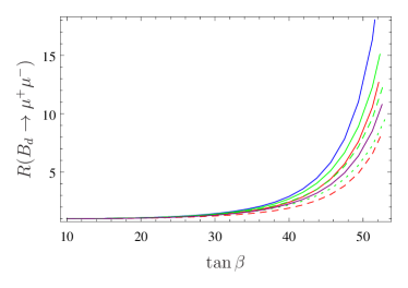
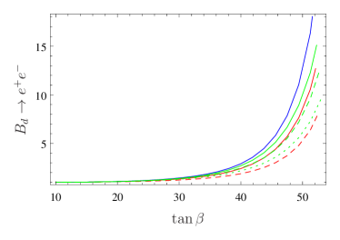
The dependence of a set of flavor observables as function of is shown in Fig. 7 and as function of in Fig. 8.
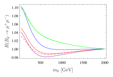

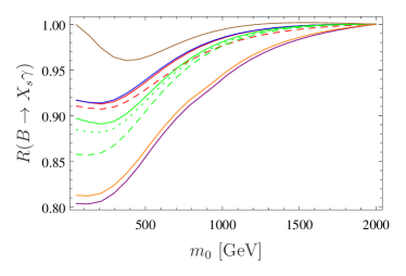
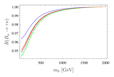
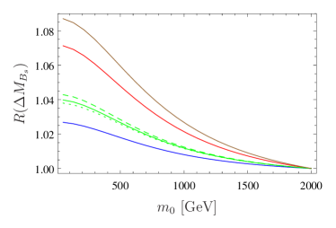
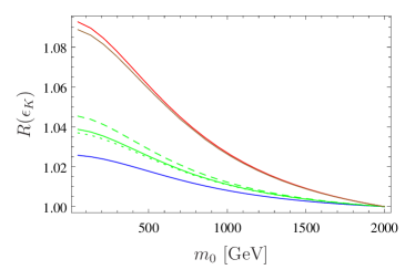
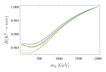
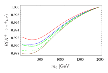
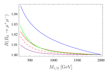
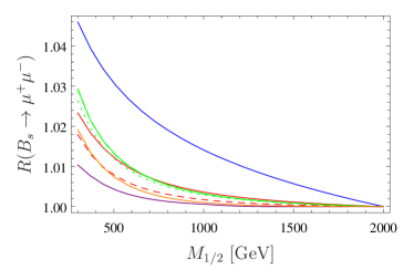
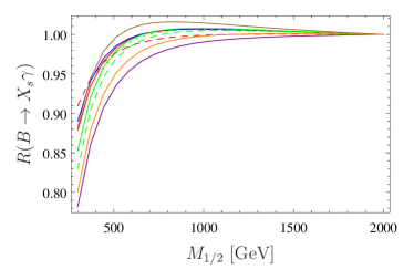
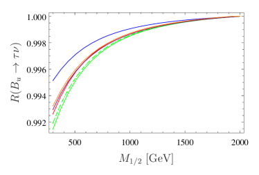


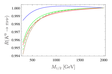

We see that all codes show in general the same dependence. However, it
is also obvious that the lines are not on top of each other but
differences are present. These differences are based on the treatment
of the resummation of the bottom Yukawa couplings, the different order
at which SM and SUSY contributions are implemented, the different
handling of the Weinberg angle, and the different level at which the
RGE running is taken into account by the tools. Even if a detailed
discussion of the differences of all codes might be very interesting
it is, of course, far beyond the scope of this paper and would require
a combined effort. The important point is that the results of
FlavorKit agree with the codes specialized for the MSSM to the same
level as those codes agree among each other. Since the FlavorKit results for all observables are based on the same generic routines it
might be even more trustworthy than human implementations of the
lengthy expressions needed to calculate these observables because it
is less error prone. Of course, known 2-loop corrections for the
MSSM which are implemented in other tools are missing.
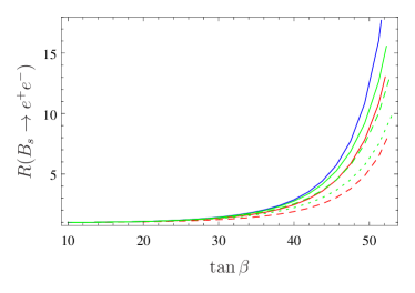
Finally, it is well known that the process has a strong dependence on the value of . We show in
Fig. 9 that this is reproduced by all codes.

7 Conclusion
We have presented FlavorKit, a new setup for the calculation of flavor observables for a wide range of BSM models. Generic expressions for the Wilson coefficients are derived with PreSARAH, a Mathematica package that makes use of FeynArts and FormCalc. The output of PreSARAH is then passed to SARAH, which generates the Fortran code that allows to calculate numerically the values of these Wilson coefficients with SPheno. The observables are derived by providing the corresponding pieces of Fortran code to SARAH, which incorporates them into the SPheno output. We made use of this code chain to fully implement a large set of important flavor observables in SARAH and SPheno. In fact, due the simplicity of this kit, the user can easily extend the list with his own observables and operators. In conclusion, FlavorKit allows the user to easily obtain analytical and numerical results for flavor observables in the BSM model of his choice.
Acknowledgments
We thank Asmaa Abada, Martin Hirsch, Farvah Mahmoudi, Manuel E. Krauss, Kilian Nickel, Ben O’Leary and Cédric Weiland for helpful discussions. FS is supported by the BMBF PT DESY Verbundprojekt 05H2013-THEORIE ’Vergleich von LHC-Daten mit supersymmetrischen Modellen’. WP is supported by the DFG, project No. PO-1337/3-1. AV is partially supported by the EXPL/FIS-NUC/0460/2013 project financed by the Portuguese FCT.
Appendix A Lagrangian
In this section we present our notation and conventions for the operators (and their corresponding Wilson coefficients) implemented in PreSARAH. Although a more complete list of flavor violating operators can be built, we will concentrate on those implemented in PreSARAH. If necessary, the user can extend it by adding his/her own operators.
The interaction Lagrangian relevant for flavor violating processes can be written as
| (7) |
The first piece contains the operators that can trigger lepton flavor violation whereas the second piece contains the operators responsible for quark flavor violation.
The general Lagrangian relevant for lepton flavor violation can be written as
| (8) |
The first term contains the interaction, given by
| (9) |
Here is the electric charge, the photon momentum, are the usual chirality projectors and denote the lepton flavors. For practical reasons, we will always consider the photonic contributions independently, and we will not include them in other vector operators. On the contrary, the - and Higgs boson contributions will be included whenever possible. Therefore, the and interaction Lagrangians will only be used for observables involving real - and Higgs bosons. These two Lagrangians can be written as
| (10) |
where is the 4-momentum, and
| (11) |
The general 4-fermion interaction Lagrangian can be written as
| (12) |
where denote the lepton flavors and , and . We omit flavor indices in the Wilson coefficients for the sake of clarity. This Lagrangian contains the most general form compatible with Lorentz invariance. The Wilson coefficients and were included in Ilakovac:2012sh , but absent in Hisano:1995cp ; Arganda:2005ji . As previously stated, the coefficients in Eq.(12) do not include photonic contributions, but they include Z-boson and scalar ones. Finally, the general four fermion interaction Lagrangian at the quark level is given by
| (13) |
where
| (14) | |||||
| (15) |
Here denotes the d-quark flavor.
Let us now consider the Lagrangian relevant for quark flavor violation. This can be written as
| (16) |
The first two terms correspond to operators that couple quark bilinears to massless gauge bosons. These are
| (17) | |||||
| (18) |
Here are matrices. The Wilson coefficients can be easily related to the usual coefficients, sometimes normalized with an additional factor. The four fermion interaction Lagrangian can be written as
| (19) |
where denote the lepton flavors. Again, we omit flavor indices in the Wilson coefficients for the sake of clarity. The four fermion interaction Lagrangian is given by
| (20) |
Here denotes the lepton flavor. should not be confused with . In the former case one has QFV operators, whereas in the latter one has LFV operators. This distinction has been made for practical reasons. The and terms of the QFV Lagrangian are
| (21) | |||||
| (22) |
Note that we have not introduced scalar or tensor operators, nor tensor ones, and that lepton flavor (denoted by the index ) is conserved in these operators. Finally, we have also included a term in the Lagrangian accounting for operators of the type and , where () is a virtual 101010We would like to emphasize that our implementation of these operators is only valid for virtual scalars and pseudoscalars. They have been introduced in order to provide the 1-loop vertices necessary for the computation of the double penguin contributions to . Therefore, they are not valid for observables in which the scalar or pseudoscalar states are real particles. scalar (pseudoscalar) state. This piece can be written as
| (23) |
Appendix B Operators available by default in the SPheno output of SARAH
The operators presented in Appendix A have been implemented by using the results of PreSARAH in SARAH. Those are exported to SPheno. We give in the following the list of all internal names for these operators, which can be used in the calculation of new flavor observables.
B.1 2-Fermion-1-Boson operators
These operators are arrays with either two or three elements. While operators involving vector bosons have always dimension , those with scalars have dimension . is the number of generations of the considered scalar and for the last index is dropped.
and
| Variable | Operator | Name | Variable | Operator | Name |
|---|---|---|---|---|---|
| CC7 | CC8 | ||||
| CC7p | CC8p |
These operators are derived by PreSARAH with the following input files
The normalization is changed to match the standard definitions by
| Variable | Operator | Name | Variable | Operator | Name |
|---|---|---|---|---|---|
| K2L | K1L | ||||
| K2R | K1R |
These operators are derived by PreSARAH with the following input files
The normalization is changed to match the standard definitions by
| Variable | Operator | Name | Variable | Operator | Name |
|---|---|---|---|---|---|
| OZ2lVL | OZ2lSL | ||||
| OZ2lVR | OZ2lSR |
In the following we omit flavor indices for the sake of simplicity. These operators are derived by PreSARAH with the following input files
| Variable | Operator | Name | Variable | Operator | Name |
|---|---|---|---|---|---|
| OH2lSL | OH2lSR |
These operators are derived by PreSARAH with the following input files
and
| Variable | Operator | Name | Variable | Operator | Name |
|---|---|---|---|---|---|
| OH2qSL | OH2qSR | ||||
| OAh2qSL | OAh2qSR |
These auxiliary 111111The and operators have been introduced to compute double penguin corrections to , where and appear as intermediate (virtual) particles. They should not be used in processes where the scalar or pseudoscalar states are real particles because the loop functions are calculated with vanishing external momenta. operators are derived by PreSARAH with the following input files
B.2 4-Fermion operators
All operators listed below carry four indices and have dimension . In addition, the user can access the different contributions of all operators from tree-level diagrams, as well as penguin and box diagrams. The name conventions are as follows: for each operator op the additional parameter exist
-
•
TSop: tree-level contributions with scalar propagator
-
•
TVop: tree-level contributions with scalar propagator
-
•
PSop: sum of penguin and self-energy contributions with scalar propagator
-
•
PVop: sum of penguin and self-energy contributions with scalar propagator
-
•
Bop: box contributions.
We will denote the 4-fermion operators involving two leptons and two down-type quarks depending on whether they lead to LFV or to QFV processes: for LFV and for QFV.
and
| Variable | Operator | Name | Variable | Operator | Name |
|---|---|---|---|---|---|
| OddllSLL | |||||
| OddllSRR | |||||
| OddllSLR | |||||
| OddllSRL | |||||
| OddllVLL | OddvvVLL | ||||
| OddllVRR | OddvvVRR | ||||
| OddllVLR | OddvvVLR | ||||
| OddllVRL | OddvvVRL | ||||
| OddllTLL | |||||
| OddllTRR | |||||
| OddllTLR | |||||
| OddllTRL |
These operators are derived by PreSARAH with the following input files
and
| Variable | Operator | Name | Variable | Operator | Name |
|---|---|---|---|---|---|
| OllddSLL | OlluuSLL | ||||
| OllddSRR | OlluuSRR | ||||
| OllddSRL | OlluuSRL | ||||
| OllddSLR | OlluuSLR | ||||
| OllddVLL | OlluuVLL | ||||
| OllddVRR | OlluuVRR | ||||
| OllddVLR | OlluuVLR | ||||
| OllddVRL | OlluuVRL | ||||
| OllddTLL | OlluuTLL | ||||
| OllddTRR | OlluuTRR | ||||
| OllddTLR | OlluuTLR | ||||
| OllddTRL | OlluuTRL |
and
| Variable | Operator | Name | Variable | Operator | Name |
|---|---|---|---|---|---|
| O4dSLL | O4lSLL | ||||
| O4dSRR | O4lSRR | ||||
| O4dSLR | O4lSLR | ||||
| O4dSRL | O4lSRL | ||||
| O4dVLL | O4lVLL | ||||
| O4dVRR | O4lVRR | ||||
| O4dVLR | O4lVLR | ||||
| O4dVRL | O4lVRL | ||||
| O4dTLL | O4lTLL | ||||
| O4dTRR | O4lTRR | ||||
| O4dTLR | O4lTLR | ||||
| O4dTRL | O4lTRL |
| Variable | Operator | Name | Variable | Operator | Name |
|---|---|---|---|---|---|
| OdulvVLL | OdulvSLL | ||||
| OdulvVRR | OdulvSRR | ||||
| OdulvVLR | OdulvSLR | ||||
| OdulvVRL | OdulvSRL |
Appendix C Application: Flavor observables implemented in SARAH
C.1 Lepton flavor observables
Lepton flavor violation in the SM or MSSM without neutrino masses vanishes exactly. Even adding Dirac neutrino masses to the SM predicts LFV rates which are far beyond the experimental reach. However, many extensions of the SM can introduce new sources for LFV of a size which is testable nowadays. The best-known examples are SUSY and non-SUSY models with high- or low-scale seesaw mechanism, models with vector-like leptons and SUSY models with -parity violation, see for instance Refs. Hisano:1995cp ; Deppisch:2002vz ; Arganda:2005ji ; Petcov:2005yh ; Antusch:2006vw ; Paradisi:2006jp ; Hirsch:2008dy ; Hirsch:2008gh ; Borzumati:2009hu ; Gross:2010ce ; Biggio:2010me ; Esteves:2010ff ; Abada:2010kj ; Abada:2011mg ; Dreiner:2012mx ; Cely:2012bz ; Hirsch:2012yv ; Davidson:2012ds ; Hirsch:2012kv ; Dinh:2012bp ; Cannoni:2013gq ; Krauss:2013gya ; Arana-Catania:2013xma ; Altmannshofer:2013zba ; Crivellin:2013hpa ; Celis:2013xja ; Moroi:2013vya ; Dinh:2013vya ; Falkowski:2013jya ; Toma:2013zsa ; Benakli:2014cia ; Teixeira:2014jza ; Celis:2014asa ; Crivellin:2014cta .
We discuss in the following the implementation of the most important LFV observables in SARAH and SPheno using the previously defined operators which are calculated by SPheno.
C.1.1
The decay width is given by Hisano:1995cp
| (24) |
where is the fine structure constant and the dipole Wilson coefficients are defined in Eq.(9).
C.1.2
The decay width is given by
Here we have defined
| (26) |
The mass of the leptons in the final state has been neglected in this formula, with the exception of the dipole terms , where an infrared divergence would otherwise occur due to the massless photon propagator. Eq.(C.1.2) is in agreement with Arganda:2005ji , but also includes the coefficients and .
C.1.3 Coherent conversion in nuclei
The conversion rate, relative to the the muon capture rate, can be expressed as Kuno:1999jp ; Arganda:2007jw
| (27) |
and are the number of protons and neutrons in the nucleus and is the effective atomic charge Chiang:1993xz . Similarly, is the Fermi constant, is the nuclear matrix element and represents the total muon capture rate. is the fine structure constant, and ( in the numerical evaluation) are the momentum and energy of the electron and is the muon mass. In the above, and (with and ) can be written in terms of effective couplings at the quark level as
| (28) |
For coherent conversion in nuclei, only scalar () and vector () couplings contribute. Furthermore, sizable contributions are expected only from the quark flavors. The numerical values of the relevant factors are Kuno:1999jp ; Kosmas:2001mv
| (29) |
Finally, the coefficients can be written in terms of the Wilson coefficients in Eqs.(9), (14) and (15) as
| (30) | |||||
| (31) | |||||
| (32) | |||||
| (33) |
Here is the quark electric charge (, ) and for d-quarks (u-quarks), with and .
C.1.4
Our analytical expressions for , where and is a pseudoscalar meson, generalize the results in Arganda:2008jj . The decay width is given by
| (34) |
where the averaged squared amplitude can be written as
| (35) |
The coefficients and can be expressed in terms of the Wilson coefficients in Eqs.(14) and (15) as
| (36) | |||||
| (37) | |||||
| (38) | |||||
| (39) | |||||
In these expressions and are the down- and up-quark masses, respectively, is the pion decay constant and the coefficients take different forms for each pseudoscalar meson Arganda:2008jj . For one has
| (40) | |||||
| (41) | |||||
| (42) |
for
| (43) | |||||
| (44) | |||||
| (45) |
and for
| (46) | |||||
| (47) | |||||
| (48) |
Here and are the masses of the neutral pion and Kaon, respectively, and is the mixing angle. In addition, .
Notice that the Wilson coefficients in Eq.(39) include all pseudoscalar and axial contributions to . Therefore, this goes beyond some well-known results in the literature, see for example Paradisi:2005tk ; Arganda:2008jj , where box contributions were neglected.
C.1.5
The decay width is given by Arganda:2004bz
C.1.6
C.2 Quark flavor observables
QFV has been observed and its description in the SM due to the CKM matrix is well established. However, the large majority of BSM models causes additional contributions which have to be studied carefully, see for instance Refs. Ciuchini:1998ix ; Buchalla:1993bv ; Misiak:1999yg ; Dedes:2001fv ; Altmannshofer:2013foa ; Dedes:2008iw ; Lunghi:2006hc ; Bobeth:2001jm ; Huber:2005ig ; Logan:2000iv ; Buras:2002vd ; Hou:1992sy ; Ibrahim:1999hh ; Barbieri:2012tu ; Altmannshofer:2012az ; Becirevic:2012fy ; Becirevic:2012jf ; Buras:2013ooa ; Dorsner:2013tla ; Descotes-Genon:2013wba ; Buras:2013dea ; Barbieri:2014tja ; Buras:2014sba ; Konig:2014iqa ; Greljo:2014dka .
We give also here a description of the implementation of the different observables using the operators present in the SPheno output of SARAH.
C.2.1
Our analytical results for follow Dedes:2008iw . The decay width to a pair of charged leptons can be written as
| (51) |
Here
| (52) | |||||
and the coefficients are defined in terms of our Wilson coefficients as121212Notice that our effective Lagrangian differs from the one in Dedes:2008iw by a factor. This relative factor has been absorbed in the expression for , see Eq.(52).
| (53) | |||||
| (54) | |||||
| (55) | |||||
| (56) |
where is the decay constant and are the masses of the quarks contained in the meson, and . In the lepton flavor conserving case, , the contribution vanishes. In this case, the results in Dedes:2008iw are in agreement with previous computations Bobeth:2002ch ; Isidori:2002qe .
C.2.2
The branching ratio for , with a cut GeV in the rest frame, can be obtained as Kagan:1998ym ; Lunghi:2006hc
| BR | (57) | ||||
where is the NNLO SM prediction Misiak:2006zs ; Misiak:2006ab , the other coefficients in Eq.(57) are found to be
| (58) |
and we have defined . Finally, the coefficients can be written in terms of in Eqs.(17) and (18) as
| (59) | |||||
| (60) | |||||
| (61) | |||||
| (62) |
where and is the Cabibbo-Kobayashi-Maskawa (CKM) matrix.
C.2.3
Our results for are based on Huber:2005ig , expanded with the addition of prime operators contributions Lunghi:private . The branching ratios for the case can be written as
| (63) | |||||
whereas for the case one gets
| (64) | |||||
Here we have defined the ratios of Wilson coefficients
| (65) |
as well as
| (66) |
C.2.4
Our results for are based on the expressions given in Altmannshofer:2013foa . The branching ratio for in the high- region, being the dilepton invariant mass squared, can be written as
| (67) |
The coefficients in Eq. (67) can be related to the ones in our generic Lagrangian as
| (68) | |||||
| (69) | |||||
| (70) | |||||
| (71) | |||||
| (72) | |||||
| (73) |
where the normalization factor was already defined after Eq. (62).
C.2.5
The branching ratio for , with , is given by Bobeth:2001jm
The sum runs over the three neutrinos and . The functions and represent the phase-space and the 1-loop QCD corrections, respectively. In case of , one needs the numerical values and . The functions and take the form
| (75) | |||||
| (76) |
Finally, Beringer:1900zz and the coefficients and are given by
| (77) | |||||
| (78) |
where is the relative factor between our Wilson coefficients and the ones in Bobeth:2001jm .
C.2.6
Following Bobeth:2001jm , the branching ratios for rare Kaon decays involving neutrinos in the final state can be written as
| (79) | |||||
| (80) |
where the sums are over the three neutrino species, is the SM NLO charm correction Buchalla:1993wq ; Buchalla:1998ba , and , the coefficients , , and take the numerical values
| (81) |
and contains the Wilson coefficients contributing to the processes, and , as
| (82) |
Here .
C.2.7
The mass difference can be written as Buras:2001mb ; Buras:2002vd
| (83) |
where , and are the mass and decay constant, respectively, is a QCD factor Buras:1990fn ; Urban:1997gw , is a non-perturbative parameter (with values and , obtained from recent lattice computations Laiho:2009eu ) and . is given by
where Buras:1990fn , , with the top quark mass, the coefficients take the numerical values
| (85) |
and the function
| (86) |
was introduced by Inami and Lim in Inami:1980fz and given, for example, in Buras:1998raa . Finally, the coefficients in Eq. (C.2.7) are related to the coefficients in Eq.(19) as
| (87) | |||||
| (88) | |||||
| (89) | |||||
| (90) | |||||
| (91) | |||||
| (92) | |||||
| (93) | |||||
| (94) |
where the factor normalizes our Wilson coefficients to the ones in Buras:2001mb ; Buras:2002vd . The corrections , and are induced by double penguin diagrams mediated by scalar and pseudoscalar states Buras:2001mb ; Buras:2002vd . These 2-loop contributions may have a sizable impact in some models, and their inclusion is necessary in order to achieve a precise result for . They can be written as
| (95) | |||||
| (96) | |||||
| (97) |
where and are defined in Eq.(23). The double penguin corrections in Eqs.(95)-(97) are obtained by summing up over all scalar and pseudoscalar states in the model.
C.2.8 and
and , the observables associated to mixing, can be written as Buras:1998raa ; Crivellin:2012jv
| (98) | |||||
| (99) |
The matrix element in Eqs. (98) and (99) is given by
| (100) | |||||
The coefficients are
| (101) | |||||
| (102) | |||||
| (103) | |||||
| (104) | |||||
| (105) |
where GeV is the energy scale at which the matrix element is computed and the Kaon decay constant. The values of the quark masses at GeV are given by MeV and MeV (see table 1 in Ciuchini:1998ix ), whereas the coefficients have the following values at GeV Buras:2001ra : , , , and .
As in Crivellin:2012jv , we treat the SM contribution separately. We define . For one just subtracts the SM contributions to , whereas for one can use the results in Herrlich:1993yv ; Herrlich:1995hh ; Herrlich:1996vf , where the relevant QCD corrections are included,
| (106) |
Here , and and are the Inami-Lim functions Inami:1980fz . was already defined in Eq. (86), whereas is given by Buras:1998raa
| (107) |
In the last expression we have kept only terms linear in . Finally, the coefficients comprise short distance QCD corrections. Their numerical values are Herrlich:1996vf 131313Note that we have chosen a value for which results from our numerical values for and , see table 5 in Herrlich:1996vf ..
C.2.9
Although , where is a pseudoscalar meson, does not violate quark flavor, we have included it in the list of observables for practical reasons, as it can be computed with the same ingredients as the QFV observables. The decay width for the process is given by Barranco:2013tba
Here is the meson decay constant, and are the masses of the quarks in the meson and the Wilson coefficients are defined in Eq.(22). The sum in Eq.(C.2.9) is over the three neutrinos (whose masses are neglected).
Each decay width is plagued by hadronic uncertainties. However, by taking the ratios
| (109) |
the hadronic uncertainties cancel out to a good approximation, allowing for a precise theoretical determination. In case of , the SM prediction includes small electromagnetic corrections that account for internal bremsstrahlung and structure-dependent effects Cirigliano:2007xi . This leads to an impressive theoretical uncertainty of , making the perfect observable to search for lepton flavor universality violation Abada:2012mc .
Appendix D Models
The following models are included in the public version of SARAH and can now be used together with the FlavorKit to get predictions for the different observables.
D.1 Supersymmetric Models
-
•
Minimal supersymmetric standard model (see Ref. Martin:1997ns and references therein)
-
–
With general flavor and CP structure (MSSM)
-
–
Without flavor violation (MSSM/NoFV)
-
–
With explicit CP violation in the Higgs sector (MSSM/CPV)
-
–
In SCKM basis (MSSM/CKM)
-
–
-
•
Singlet extensions:
-
–
Next-to-minimal supersymmetric standard model (NMSSM, NMSSM/NoFV, NMSSM/CPV, NMSSM/CKM) (see Refs. Maniatis:2009re ; Ellwanger:2009dp and references therein)
-
–
near-to-minimal supersymmetric standard model (near-MSSM) Barger:2006dh
-
–
General singlet extended, supersymmetric standard model (SMSSM) Barger:2006dh ; Ross:2012nr
-
–
DiracNMSSM (DiracNMSSM) Lu:2013cta ; Kaminska:2014wia
-
–
-
•
Triplet extensions
-
–
Triplet extended MSSM (TMSSM) DiChiara:2008rg
-
–
Triplet extended NMSSM (TNMSSM) Agashe:2011ia
-
–
-
•
Models with -parity violation Hall:1983id ; Dreiner:1997uz ; Allanach:2003eb ; Bhattacharyya:1997vv ; Barger:1989rk ; Allanach:1999ic ; Hirsch:2000ef ; Barbier:2004ez
-
–
bilinear RpV (MSSM-RpV/Bi)
-
–
Lepton number violation (MSSM-RpV/LnV)
-
–
Only trilinear lepton number violation (MSSM-RpV/TriLnV)
-
–
Baryon number violation (MSSM-RpV/BnV)
-
–
SSM (munuSSM) LopezFogliani:2005yw ; Bartl:2009an
-
–
-
•
Additional
-
–
-extended MSSM (UMSSM) Barger:2006dh
-
–
secluded MSSM (secluded-MSSM) Chiang:2009fs
-
–
minimal model (B-L-SSM) Khalil:2007dr ; FileviezPerez:2010ek ; O'Leary:2011yq ; Basso:2012gz
-
–
minimal singlet-extended model (N-B-L-SSM)
-
–
-
•
SUSY-scale seesaw extensions
-
–
inverse seesaw (inverse-Seesaw) Malinsky:2005bi ; BhupalDev:2012ru
-
–
linear seesaw (LinSeesaw) Malinsky:2005bi ; DeRomeri:2012qd
-
–
singlet extended inverse seesaw (inverse-Seesaw-NMSSM) Gogoladze:2012jp
-
–
inverse seesaw with gauge group (B-L-SSM-IS) Basso:2012ew
-
–
minimal model with inverse seesaw (BLRinvSeesaw) Hirsch:2011hg ; Hirsch:2012kv
-
–
-
•
Models with Dirac Gauginos
-
–
MSSM/NMSSM with Dirac Gauginos (DiracGauginos) Belanger:2009wf ; Benakli:2010gi ; Benakli:2012cy
-
–
minimal -Symmetric SSM (MRSSM) Kribs:2007ac
-
–
Minimal Dirac Gaugino supersymmetric standard model (MDGSSM) Benakli:2014cia
-
–
-
•
High-scale extensions
-
–
Seesaw 1 - 3 ( version) , (Seesaw1,Seesaw2,Seesaw3) Borzumati:2009hu ; Rossi:2002zb ; Hirsch:2008dy ; Esteves:2009vg ; Esteves:2010ff
-
–
Left/right model (LR) (Omega) Esteves:2010si ; Esteves:2011gk
-
–
Quiver model (QEW12, QEWmld2L3) Bharucha:2013ela
-
–
D.2 Non-Supersymmetric Models
-
•
Standard Model (SM) (SM), Standard model in CKM basis (SM/CKM) (see for instance Ref. Hollik:2010id and references therein)
-
•
inert Higgs doublet model (Inert) LopezHonorez:2006gr
-
•
B-L extended SM (B-L-SM) Emam:2007dy ; Basso:2008iv ; Basso:2009hf
-
•
B-L extended SM with inverse seesaw (B-L-SM-IS) Khalil:2010iu
-
•
SM extended by a scalar color octet (SM-8C) Patel:2013zla
-
•
Two Higgs doublet model (THDM) (see for instance Ref. Branco:2011iw and references therein)
-
•
Singlet extended SM (SSM) O'Connell:2006wi
-
•
Singlet Scalar DM (SSDM) Goudelis:2009zz
References
- (1) ATLAS Collaboration, G. Aad et al., Phys.Lett. B716 (2012), 1–29, [1207.7214].
- (2) CMS Collaboration, S. Chatrchyan et al., Phys.Lett. B716 (2012), 30–61, [1207.7235].
- (3) ATLAS Collaboration, CDF Collaboration, CMS Collaboration, D0 Collaboration, (2014), 1403.4427.
- (4) D. Buttazzo, G. Degrassi, P. P. Giardino, G. F. Giudice, F. Sala, et al., JHEP 1312 (2013), 089, [1307.3536].
- (5) F. Mahmoudi, Comput.Phys.Commun. 178 (2008), 745–754, [0710.2067].
- (6) F. Mahmoudi, Comput.Phys.Commun. 180 (2009), 1579–1613, [0808.3144].
- (7) F. Mahmoudi, Comput.Phys.Commun. 180 (2009), 1718–1719.
- (8) J. Rosiek, P. Chankowski, A. Dedes, S. Jager, and P. Tanedo, Comput.Phys.Commun. 181 (2010), 2180–2205, [1003.4260].
- (9) A. Crivellin, J. Rosiek, P. Chankowski, A. Dedes, S. Jaeger, et al., Comput.Phys.Commun. 184 (2013), 1004–1032, [1203.5023].
- (10) U. Ellwanger and C. Hugonie, Comput.Phys.Commun. 177 (2007), 399–407, [hep-ph/0612134].
- (11) G. Belanger, F. Boudjema, A. Pukhov, and A. Semenov, Comput.Phys.Commun. 149 (2002), 103–120, [hep-ph/0112278].
- (12) G. Belanger, F. Boudjema, A. Pukhov, and A. Semenov, Comput.Phys.Commun. 174 (2006), 577–604, [hep-ph/0405253].
- (13) G. Belanger, F. Boudjema, A. Pukhov, and A. Semenov, Comput.Phys.Commun. 176 (2007), 367–382, [hep-ph/0607059].
- (14) G. Belanger, F. Boudjema, A. Pukhov, and A. Semenov, Comput.Phys.Commun. 180 (2009), 747–767, [0803.2360].
- (15) G. Belanger, F. Boudjema, A. Pukhov, and A. Semenov, Comput.Phys.Commun. 185 (2014), 960–985, [1305.0237].
- (16) G. Degrassi, P. Gambino, and P. Slavich, Comput.Phys.Commun. 179 (2008), 759–771, [0712.3265].
- (17) B. Murakami, Comput.Phys.Commun. 185 (2014), 622–637, [1302.4469].
- (18) D. Chowdhury, R. Garani, and S. K. Vempati, Comput.Phys.Commun. 184 (2013), 899–918, [1109.3551].
- (19) F. E. Paige, S. D. Protopopescu, H. Baer, and X. Tata, (2003), hep-ph/0312045.
- (20) H. Baer, C. Balazs, A. Belyaev, R. Dermisek, A. Mafi, et al., Nucl.Instrum.Meth. A502 (2003), 560–563.
- (21) H. Baer, F. E. Paige, S. D. Protopopescu, and X. Tata, (1999), hep-ph/0001086.
- (22) F. E. Paige, S. D. Protopescu, H. Baer, and X. Tata, (1998), hep-ph/9810440.
- (23) F. E. Paige, S. D. Protopopescu, H. Baer, and X. Tata, (1998), hep-ph/9804321.
- (24) H. Baer, F. E. Paige, S. D. Protopopescu, and X. Tata, (1993), hep-ph/9305342.
- (25) W. Porod, Comput.Phys.Commun. 153 (2003), 275–315, [hep-ph/0301101].
- (26) W. Porod and F. Staub, Comput.Phys.Commun. 183 (2012), 2458–2469, [1104.1573].
- (27) F. Staub, (2008), 0806.0538.
- (28) F. Staub, Comput.Phys.Commun. 181 (2010), 1077–1086, [0909.2863].
- (29) F. Staub, Comput.Phys.Commun. 182 (2011), 808–833, [1002.0840].
- (30) F. Staub, Computer Physics Communications 184 (2013), pp. 1792–1809, [1207.0906].
- (31) F. Staub, Comput.Phys.Commun. 185 (2014), 1773–1790, [1309.7223].
- (32) H. Dreiner, K. Nickel, F. Staub, and A. Vicente, Phys.Rev. D86 (2012), 015003, [1204.5925].
- (33) H. Dreiner, K. Nickel, W. Porod, and F. Staub, Comput.Phys.Commun. 184 (2013), 2604–2617, [1212.5074].
- (34) H. Dreiner, K. Nickel, and F. Staub, Phys.Rev. D88 (2013), 115001, [1309.1735].
- (35) T. Hahn and M. Perez-Victoria, Comput.Phys.Commun. 118 (1999), 153–165, [hep-ph/9807565].
- (36) T. Hahn, Comput.Phys.Commun. 140 (2001), 418–431, [hep-ph/0012260].
- (37) T. Hahn, Nucl.Phys.Proc.Suppl. 89 (2000), 231–236, [hep-ph/0005029].
- (38) T. Hahn, Nucl.Phys.Proc.Suppl. 135 (2004), 333–337, [hep-ph/0406288].
- (39) T. Hahn, eConf C050318 (2005), 0604, [hep-ph/0506201].
- (40) B. C. Nejad, T. Hahn, J. N. Lang, and E. Mirabella, (2013), 1310.0274.
- (41) E. Ma and A. Pramudita, Phys.Rev. D24 (1981), 1410.
- (42) J. Hisano, T. Moroi, K. Tobe, and M. Yamaguchi, Phys.Rev. D53 (1996), 2442–2459, [hep-ph/9510309].
- (43) A. Bednyakov and S. Tanyildizi, (2013), 1311.5546.
- (44) T. Ohl, Comput.Phys.Commun. 90 (1995), 340–354, [hep-ph/9505351].
- (45) F. Staub, T. Ohl, W. Porod, and C. Speckner, Comput.Phys.Commun. 183 (2012), 2165–2206, [1109.5147].
- (46) A. Crivellin, L. Hofer, and J. Rosiek, JHEP 1107 (2011), 017, [1103.4272].
- (47) A. J. Buras, M. Jamin, and P. H. Weisz, Nucl.Phys. B347 (1990), 491–536.
- (48) G. Buchalla and A. J. Buras, Nucl.Phys. B412 (1994), 106–142, [hep-ph/9308272].
- (49) M. Ciuchini, E. Franco, and V. Gimenez, Phys.Lett. B388 (1996), 167–172, [hep-ph/9608204].
- (50) A. J. Buras, P. Gambino, and U. A. Haisch, Nucl.Phys. B570 (2000), 117–154, [hep-ph/9911250].
- (51) M. Misiak and M. Steinhauser, Nucl.Phys. B764 (2007), 62–82, [hep-ph/0609241].
- (52) A. J. Buras, A. Czarnecki, M. Misiak, and J. Urban, Nucl.Phys. B631 (2002), 219–238, [hep-ph/0203135].
- (53) R. Boughezal, M. Czakon, and T. Schutzmeier, JHEP 0709 (2007), 072, [0707.3090].
- (54) A. J. Buras and J. Girrbach, JHEP 1203 (2012), 052, [1201.1302].
- (55) F. Mahmoudi, S. Heinemeyer, A. Arbey, A. Bharucha, T. Goto, et al., Comput.Phys.Commun. 183 (2012), 285–298, [1008.0762].
- (56) A. Ilakovac and A. Pilaftsis, Nucl.Phys. B437 (1995), 491, [hep-ph/9403398].
- (57) A. Ilakovac, A. Pilaftsis, and L. Popov, Phys.Rev. D87 (2013), no. 5, 053014, [1212.5939].
- (58) E. Arganda and M. J. Herrero, Phys.Rev. D73 (2006), 055003, [hep-ph/0510405].
- (59) F. Deppisch, H. Pas, A. Redelbach, R. Ruckl, and Y. Shimizu, Eur.Phys.J. C28 (2003), 365–374, [hep-ph/0206122].
- (60) S. Petcov, T. Shindou, and Y. Takanishi, Nucl.Phys. B738 (2006), 219–242, [hep-ph/0508243].
- (61) S. Antusch, E. Arganda, M. Herrero, and A. Teixeira, JHEP 0611 (2006), 090, [hep-ph/0607263].
- (62) P. Paradisi, JHEP 0608 (2006), 047, [hep-ph/0601100].
- (63) M. Hirsch, J. Valle, W. Porod, J. Romao, and A. Villanova del Moral, Phys.Rev. D78 (2008), 013006, [0804.4072].
- (64) M. Hirsch, S. Kaneko, and W. Porod, Phys.Rev. D78 (2008), 093004, [0806.3361].
- (65) F. Borzumati and T. Yamashita, Prog.Theor.Phys. 124 (2010), 761–868, [0903.2793].
- (66) E. Gross, D. Grossman, Y. Nir, and O. Vitells, Phys.Rev. D81 (2010), 055013, [1001.2883].
- (67) C. Biggio and L. Calibbi, JHEP 1010 (2010), 037, [1007.3750].
- (68) J. Esteves, J. Romao, M. Hirsch, F. Staub, and W. Porod, Phys.Rev. D83 (2011), 013003, [1010.6000].
- (69) A. Abada, A. Figueiredo, J. Romao, and A. Teixeira, JHEP 1010 (2010), 104, [1007.4833].
- (70) A. Abada, A. Figueiredo, J. Romao, and A. Teixeira, JHEP 1108 (2011), 099, [1104.3962].
- (71) C. G. Cely, A. Ibarra, E. Molinaro, and S. Petcov, Phys.Lett. B718 (2013), 957–964, [1208.3654].
- (72) M. Hirsch, W. Porod, C. Weiss, and F. Staub, Phys.Rev. D87 (2013), 013010, [1211.0289].
- (73) S. Davidson and P. Verdier, Phys.Rev. D86 (2012), 111701, [1211.1248].
- (74) M. Hirsch, W. Porod, L. Reichert, and F. Staub, Phys.Rev. D86 (2012), 093018, [1206.3516].
- (75) D. Dinh, A. Ibarra, E. Molinaro, and S. Petcov, JHEP 1208 (2012), 125, [1205.4671].
- (76) M. Cannoni, J. Ellis, M. E. Gomez, and S. Lola, Phys.Rev. D88 (2013), 075005, [1301.6002].
- (77) M. E. Krauss, W. Porod, F. Staub, A. Abada, A. Vicente, et al., (2013), 1312.5318.
- (78) M. Arana-Catania, E. Arganda, and M. Herrero, JHEP 1309 (2013), 160, [1304.3371].
- (79) W. Altmannshofer, M. Bauer, and M. Carena, JHEP 1401 (2014), 060, [1308.1987].
- (80) A. Crivellin, S. Najjari, and J. Rosiek, JHEP 1404 (2014), 167, [1312.0634].
- (81) A. Celis, V. Cirigliano, and E. Passemar, Phys.Rev. D89 (2014), 013008, [1309.3564].
- (82) T. Moroi, M. Nagai, and T. T. Yanagida, Phys.Lett. B728 (2014), 342–346, [1305.7357].
- (83) D. Dinh and S. Petcov, JHEP 1309 (2013), 086, [1308.4311].
- (84) A. Falkowski, D. M. Straub, and A. Vicente, (2013), 1312.5329.
- (85) T. Toma and A. Vicente, JHEP 1401 (2014), 160, [1312.2840].
- (86) K. Benakli, M. Goodsell, F. Staub, and W. Porod, (2014), 1403.5122.
- (87) A. Teixeira, A. Abada, A. Figueiredo, and J. Romao, (2014), 1402.1426.
- (88) A. Celis, V. Cirigliano, and E. Passemar, (2014), 1403.5781.
- (89) A. Crivellin, M. Hoferichter, and M. Procura, (2014), 1404.7134.
- (90) Y. Kuno and Y. Okada, Rev.Mod.Phys. 73 (2001), 151–202, [hep-ph/9909265].
- (91) E. Arganda, M. Herrero, and A. Teixeira, JHEP 0710 (2007), 104, [0707.2955].
- (92) H. Chiang, E. Oset, T. Kosmas, A. Faessler, and J. Vergados, Nucl.Phys. A559 (1993), 526–542.
- (93) T. Kosmas, S. Kovalenko, and I. Schmidt, Phys.Lett. B511 (2001), 203, [hep-ph/0102101].
- (94) E. Arganda, M. Herrero, and J. Portoles, JHEP 0806 (2008), 079, [0803.2039].
- (95) P. Paradisi, JHEP 0602 (2006), 050, [hep-ph/0508054].
- (96) E. Arganda, A. M. Curiel, M. J. Herrero, and D. Temes, Phys.Rev. D71 (2005), 035011, [hep-ph/0407302].
- (97) X.-J. Bi, Y.-B. Dai, and X.-Y. Qi, Phys.Rev. D63 (2001), 096008, [hep-ph/0010270].
- (98) M. Ciuchini, V. Lubicz, L. Conti, A. Vladikas, A. Donini, et al., JHEP 9810 (1998), 008, [hep-ph/9808328].
- (99) G. Buchalla and A. J. Buras, Nucl.Phys. B400 (1993), 225–239.
- (100) M. Misiak and J. Urban, Phys.Lett. B451 (1999), 161–169, [hep-ph/9901278].
- (101) A. Dedes, H. K. Dreiner, and U. Nierste, Phys.Rev.Lett. 87 (2001), 251804, [hep-ph/0108037].
- (102) W. Altmannshofer and D. M. Straub, Eur.Phys.J. C73 (2013), 2646, [1308.1501].
- (103) A. Dedes, J. Rosiek, and P. Tanedo, Phys.Rev. D79 (2009), 055006, [0812.4320].
- (104) E. Lunghi and J. Matias, JHEP 0704 (2007), 058, [hep-ph/0612166].
- (105) C. Bobeth, A. J. Buras, F. Kruger, and J. Urban, Nucl.Phys. B630 (2002), 87–131, [hep-ph/0112305].
- (106) T. Huber, E. Lunghi, M. Misiak, and D. Wyler, Nucl.Phys. B740 (2006), 105–137, [hep-ph/0512066].
- (107) H. E. Logan and U. Nierste, Nucl.Phys. B586 (2000), 39–55, [hep-ph/0004139].
- (108) A. J. Buras, P. H. Chankowski, J. Rosiek, and L. Slawianowska, Nucl.Phys. B659 (2003), 3, [hep-ph/0210145].
- (109) W.-S. Hou, Phys.Rev. D48 (1993), 2342–2344.
- (110) T. Ibrahim and P. Nath, Phys.Rev. D61 (2000), 095008, [hep-ph/9907555].
- (111) R. Barbieri, D. Buttazzo, F. Sala, D. M. Straub, and A. Tesi, JHEP 1305 (2013), 069, [1211.5085].
- (112) W. Altmannshofer and D. M. Straub, JHEP 1208 (2012), 121, [1206.0273].
- (113) D. Becirevic, N. Kosnik, F. Mescia, and E. Schneider, Phys.Rev. D86 (2012), 034034, [1205.5811].
- (114) D. Becirevic, N. Kosnik, and A. Tayduganov, Phys.Lett. B716 (2012), 208–213, [1206.4977].
- (115) A. J. Buras and J. Girrbach, (2013), 1306.3775.
- (116) I. Dorsner, S. Fajfer, N. Kosnik, and I. Nisandzic, JHEP 1311 (2013), 084, [1306.6493].
- (117) S. Descotes-Genon, J. Matias, and J. Virto, Phys.Rev. D88 (2013), 074002, [1307.5683].
- (118) A. J. Buras, F. De Fazio, and J. Girrbach, JHEP 1402 (2014), 112, [1311.6729].
- (119) R. Barbieri, D. Buttazzo, F. Sala, and D. M. Straub, (2014), 1402.6677.
- (120) A. J. Buras, F. De Fazio, and J. Girrbach, (2014), 1404.3824.
- (121) M. König, M. Neubert, and D. M. Straub, (2014), 1403.2756.
- (122) A. Greljo, J. F. Kamenik, and J. Kopp, (2014), 1404.1278.
- (123) C. Bobeth, T. Ewerth, F. Kruger, and J. Urban, Phys.Rev. D66 (2002), 074021, [hep-ph/0204225].
- (124) G. Isidori and A. Retico, JHEP 0209 (2002), 063, [hep-ph/0208159].
- (125) A. L. Kagan and M. Neubert, Eur.Phys.J. C7 (1999), 5–27, [hep-ph/9805303].
- (126) M. Misiak, H. Asatrian, K. Bieri, M. Czakon, A. Czarnecki, et al., Phys.Rev.Lett. 98 (2007), 022002, [hep-ph/0609232].
- (127) E. Lunghi, private communication.
- (128) Particle Data Group, J. Beringer et al., Phys.Rev. D86 (2012), 010001.
- (129) G. Buchalla and A. J. Buras, Nucl.Phys. B548 (1999), 309–327, [hep-ph/9901288].
- (130) A. J. Buras, P. H. Chankowski, J. Rosiek, and L. Slawianowska, Nucl.Phys. B619 (2001), 434–466, [hep-ph/0107048].
- (131) J. Urban, F. Krauss, U. Jentschura, and G. Soff, Nucl.Phys. B523 (1998), 40–58, [hep-ph/9710245].
- (132) J. Laiho, E. Lunghi, and R. S. Van de Water, Phys.Rev. D81 (2010), 034503, [0910.2928].
- (133) T. Inami and C. Lim, Prog.Theor.Phys. 65 (1981), 297.
- (134) A. J. Buras, (1998), 281–539, hep-ph/9806471.
- (135) A. J. Buras, S. Jager, and J. Urban, Nucl.Phys. B605 (2001), 600–624, [hep-ph/0102316].
- (136) S. Herrlich and U. Nierste, Nucl.Phys. B419 (1994), 292–322, [hep-ph/9310311].
- (137) S. Herrlich and U. Nierste, Phys.Rev. D52 (1995), 6505–6518, [hep-ph/9507262].
- (138) S. Herrlich and U. Nierste, Nucl.Phys. B476 (1996), 27–88, [hep-ph/9604330].
- (139) J. Barranco, D. Delepine, V. Gonzalez Macias, and L. Lopez-Lozano, Phys.Lett. B731 (2014), 36–42, [1303.3896].
- (140) V. Cirigliano and I. Rosell, Phys.Rev.Lett. 99 (2007), 231801, [0707.3439].
- (141) A. Abada, D. Das, A. Teixeira, A. Vicente, and C. Weiland, JHEP 1302 (2013), 048, [1211.3052].
- (142) S. P. Martin, (1997), hep-ph/9709356.
- (143) M. Maniatis, Int.J.Mod.Phys. A25 (2010), 3505–3602, [0906.0777].
- (144) U. Ellwanger, C. Hugonie, and A. M. Teixeira, Phys.Rept. 496 (2010), 1–77, [0910.1785].
- (145) V. Barger, P. Langacker, H.-S. Lee, and G. Shaughnessy, Phys.Rev. D73 (2006), 115010, [hep-ph/0603247].
- (146) G. G. Ross, K. Schmidt-Hoberg, and F. Staub, JHEP 1208 (2012), 074, [1205.1509].
- (147) X. Lu, H. Murayama, J. T. Ruderman, and K. Tobioka, (2013), 1308.0792.
- (148) A. Kaminska, G. G. Ross, K. Schmidt-Hoberg, and F. Staub, (2014), 1401.1816.
- (149) S. Di Chiara and K. Hsieh, Phys.Rev. D78 (2008), 055016, [0805.2623].
- (150) K. Agashe, A. Azatov, A. Katz, and D. Kim, Phys.Rev. D84 (2011), 115024, [1109.2842].
- (151) L. J. Hall and M. Suzuki, Nucl.Phys. B231 (1984), 419.
- (152) H. K. Dreiner, (1997), hep-ph/9707435.
- (153) B. Allanach, A. Dedes, and H. Dreiner, Phys.Rev. D69 (2004), 115002, [hep-ph/0309196].
- (154) G. Bhattacharyya, (1997), hep-ph/9709395.
- (155) V. D. Barger, G. Giudice, and T. Han, Phys.Rev. D40 (1989), 2987.
- (156) B. Allanach, A. Dedes, and H. K. Dreiner, Phys.Rev. D60 (1999), 075014, [hep-ph/9906209].
- (157) M. Hirsch, M. Diaz, W. Porod, J. Romao, and J. Valle, Phys.Rev. D62 (2000), 113008, [hep-ph/0004115].
- (158) R. Barbier, C. Berat, M. Besancon, M. Chemtob, A. Deandrea, et al., Phys.Rept. 420 (2005), 1–202, [hep-ph/0406039].
- (159) D. Lopez-Fogliani and C. Munoz, Phys.Rev.Lett. 97 (2006), 041801, [hep-ph/0508297].
- (160) A. Bartl, M. Hirsch, A. Vicente, S. Liebler, and W. Porod, JHEP 0905 (2009), 120, [0903.3596].
- (161) C.-W. Chiang and E. Senaha, JHEP 1006 (2010), 030, [0912.5069].
- (162) S. Khalil and A. Masiero, Phys.Lett. B665 (2008), 374–377, [0710.3525].
- (163) P. Fileviez Perez and S. Spinner, Phys.Rev. D83 (2011), 035004, [1005.4930].
- (164) B. O’Leary, W. Porod, and F. Staub, JHEP 1205 (2012), 042, [1112.4600].
- (165) L. Basso, B. O’Leary, W. Porod, and F. Staub, JHEP 1209 (2012), 054, [1207.0507].
- (166) M. Malinsky, J. Romao, and J. Valle, Phys.Rev.Lett. 95 (2005), 161801, [hep-ph/0506296].
- (167) P. Bhupal Dev, S. Mondal, B. Mukhopadhyaya, and S. Roy, JHEP 1209 (2012), 110, [1207.6542].
- (168) V. De Romeri and M. Hirsch, JHEP 1212 (2012), 106, [1209.3891].
- (169) I. Gogoladze, B. He, and Q. Shafi, Phys.Lett. B718 (2013), 1008–1013, [1209.5984].
- (170) L. Basso, A. Belyaev, D. Chowdhury, M. Hirsch, S. Khalil, et al., Comput.Phys.Commun. 184 (2013), 698–719, [1206.4563].
- (171) M. Hirsch, M. Malinsky, W. Porod, L. Reichert, and F. Staub, JHEP 1202 (2012), 084, [1110.3037].
- (172) G. Belanger, K. Benakli, M. Goodsell, C. Moura, and A. Pukhov, JCAP 0908 (2009), 027, [0905.1043].
- (173) K. Benakli and M. Goodsell, Nucl.Phys. B840 (2010), 1–28, [1003.4957].
- (174) K. Benakli, M. D. Goodsell, and F. Staub, JHEP 1306 (2013), 073, [1211.0552].
- (175) G. D. Kribs, E. Poppitz, and N. Weiner, Phys.Rev. D78 (2008), 055010, [0712.2039].
- (176) A. Rossi, Phys.Rev. D66 (2002), 075003, [hep-ph/0207006].
- (177) J. Esteves, J. Romao, A. Villanova del Moral, M. Hirsch, J. Valle, et al., JHEP 0905 (2009), 003, [0903.1408].
- (178) J. Esteves, J. Romao, M. Hirsch, A. Vicente, W. Porod, et al., JHEP 1012 (2010), 077, [1011.0348].
- (179) J. Esteves, J. Romao, M. Hirsch, W. Porod, F. Staub, et al., JHEP 1201 (2012), 095, [1109.6478].
- (180) A. Bharucha, A. Goudelis, and M. McGarrie, (2013), 1310.4500.
- (181) W. Hollik, (2010), 1012.3883.
- (182) L. Lopez Honorez, E. Nezri, J. F. Oliver, and M. H. Tytgat, JCAP 0702 (2007), 028, [hep-ph/0612275].
- (183) W. Emam and S. Khalil, Eur.Phys.J. C52 (2007), 625–633, [0704.1395].
- (184) L. Basso, A. Belyaev, S. Moretti, and C. H. Shepherd-Themistocleous, Phys.Rev. D80 (2009), 055030, [0812.4313].
- (185) L. Basso, A. Belyaev, S. Moretti, and G. M. Pruna, JHEP 0910 (2009), 006, [0903.4777].
- (186) S. Khalil, Phys.Rev. D82 (2010), 077702, [1004.0013].
- (187) H. H. Patel, M. J. Ramsey-Musolf, and M. B. Wise, Phys.Rev. D88 (2013), no. 1, 015003, [1303.1140].
- (188) G. Branco, P. Ferreira, L. Lavoura, M. Rebelo, M. Sher, et al., Phys.Rept. 516 (2012), 1–102, [1106.0034].
- (189) D. O’Connell, M. J. Ramsey-Musolf, and M. B. Wise, Phys.Rev. D75 (2007), 037701, [hep-ph/0611014].
- (190) A. Goudelis, Y. Mambrini, and C. Yaguna, JCAP 0912 (2009), 008, [0909.2799].