Rapidly increasing collimation and magnetic field changes of a protostellar H₂O maser outflow

Abstract

Context. W75N(B) is a massive star-forming region that contains three radio continuum sources (VLA 1, VLA 2, and VLA 3), which are thought to be three massive young stellar objects at three different evolutionary stages. VLA 1 is the most evolved and VLA 2 the least evolved source. The 22 GHz H₂O masers associated with VLA 1 and VLA 2 have been mapped at several epochs over eight years. While the H₂O masers in VLA 1 show a persistent linear distribution along a radio jet, those in VLA 2 are distributed around an expanding shell. Furthermore, H₂O maser polarimetric measurements revealed magnetic fields aligned with the two structures.

Aims. Using new polarimetric observations of H₂O masers, we aim to confirm the elliptical expansion of the shell-like structure around VLA 2 and, at the same time, to determine if the magnetic fields around the two sources have changed.

Methods. The NRAO Very Long Baseline Array was used to measure the linear polarization and the Zeeman-splitting of the 22 GHz H₂O masers towards the massive star-forming region W75N(B).

Results. The H₂O maser distribution around VLA 1 is unchanged from that previously observed. We made an elliptical fit of the H₂O masers around VLA 2. We find that the shell-like structure is still expanding along the direction parallel to the thermal radio jet of VLA 1. While the magnetic field around VLA 1 has not changed in the past $\sim$7 years, the magnetic field around VLA 2 has changed its orientation according to the new direction of the major-axis of the shell-like structure and it is now aligned with the magnetic field in VLA 1.

1 Introduction

The formation of massive stars and the evolution of associated protostellar outflow is still a matter of debate (e.g., Beuther & Shepherd beu05 (2005); Zinnecker & Yorke zin07 (2007)). Beuther & Shepherd (beu05 (2005)) propose an evolutionary scenario in which well-collimated outflows occur in the very early phases of high-mass star formation (HMSF) and, in their evolution, the outflows get progressively less collimated because of the build-up of an H ii region. Recent magnetohydrodynamics (MHD) simulations show that magnetic fields coupled to prestellar disks drive outflows, which could also be poorly collimated at very early stages of HMSF, depending on the magnetic field strength (e.g., Banerjee & Pudritz ban07 (2007), Seifried et al. sei11 (2011, 2012)).
Although multi-epoch Very Long Baseline Interferometry (VLBI) observations of 22 GHz H₂O masers were successful in identifying jets/outflows (Goddi et al. god05 (2005); Moscadelli et al. mos07 (2007); Sanna et al. san10 (2010)), monitoring studies of outflow formation and magnetic field evolution at early stages of HMSF are still lacking. Fortunately, one very singular case where we can do both studies at the same time does exist; this is W75N(B).
The active massive star-forming region W75N(B) is located at a distance of $1.3$ kpc (Rygl et al. ryg12 (2012)) that contains three massive young stellar objects (YSOs) within an area of $\sim 1.5^{\prime\prime}\times 1.5^{\prime\prime}$ ($\sim 2000\leavevmode\nobreak\ \rm{au}\times 2000\leavevmode\nobreak\ \rm{au}$), named VLA 1, VLA 2, and VLA 3 (Torrelles et al. tor97 (1997); Carrasco-González et al. gon10 (2010)). The sources VLA 1 and VLA 3 show elongated radio continuum emission consistent with a thermal radio jet, while VLA 2, which is located between VLA 1 and VLA 3, shows unresolved continuum emission ($\leq 0.08^{\prime\prime}$) of unknown nature (Torrelles et al. tor97 (1997)). The three sources are thought to be YSOs at three different evolutionary stages; in particular, VLA 1 is the most evolved and VLA 2 the least evolved (Torrelles et al. tor97 (1997)). Several maser species have been detected towards W75N(B) (e.g., Baart et al. baa86 (1986); Torrelles et al. tor97 (1997); Surcis et al. sur09 (2009)). In particular, the 22 GHz H₂O masers have been monitored over a period of eight years from 1999 to 2007 (e.g., Torrelles et al. tor03 (2003), hereafter T03; Surcis et al. sur11 (2011), hereafter S11; Kim et al. kim13 (2013), hereafter K13).
Remarkably, while the H₂O masers in VLA 1 trace a collimated thermal radio jet of $\sim 1^{\prime\prime}$ (1300 au) with $\rm{PA_{jet}}\approx+43$^∘ (Torrelles et al. tor97 (1997)), those around VLA 2 are tracing an expanding shell that evolved from a quasi-spherical to a collimated structure over eight years (T03, S11, K13). Moreover, S11 analyzed the polarized emission of 22 GHz H₂O masers and found that the magnetic field around VLA 1 and VLA 2 (separated by just 1300 au) has different orientation and strength.
Therefore, we propose W75N(B) as the best case known where the transition from a non-collimated to a well-collimated outflow in the very early phase of HMSF can be observed in “real time”. In this letter, we present new polarimetric VLBI observations of H₂O masers to confirm the elliptical expansion of the shell-like structure around VLA 2 as well as to determine possible changes in the magnetic field.

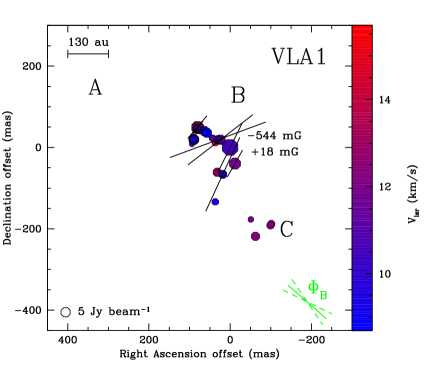
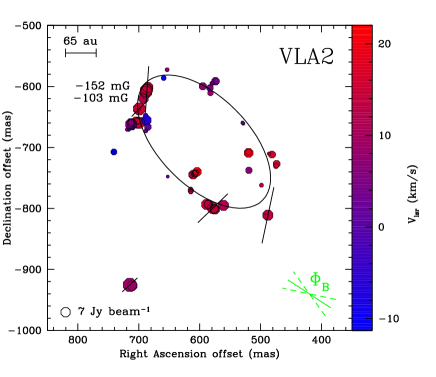
Figure 1: A close-up view of the 22 GHz H₂O maser features detected around the radio source VLA 1 (left panel) and VLA 2 (right panel). The reference position is $\alpha_{2000}=20^{\rm{h}}38^{\rm{m}}36^{\rm{s}}\!.435$ and $\delta_{2000}=42^{\circ}37^{\prime}34^{\prime\prime}\!\!.84$ (see Sect. 2). The octagonal symbols are the identified maser features in the present work scaled logarithmically according to their peak flux density (Tables 4 and 5, online material). The linear polarization vectors, scaled logarithmically according to polarization fraction $P_{\rm{l}}$, are overplotted. In the bottom-right corner of both panels the error-weighted orientation of the magnetic field ($\Phi_{\rm{B}}$, see Sect. 3) is also reported; the two dashed segments indicate the uncertainties. The ellipse drawn in the right panel is the result of the best fit of the H₂O masers detected in the present work (epoch 2012.54). Its parameters are listed in Table 3. The estimated values of the magnetic field strength are also shown in both panels next to the corresponding H₂O maser.

2 Observations and analysis

The star-forming region W75N(B) was observed in the $6_{16}-5_{23}$ transition of H₂O (rest frequency: 22.23508 GHz) with the NRAO VLBA on July 15, 2012. The observations were made in full polarization mode using a bandwidth of 4 MHz to cover a velocity range of $\sim 54$ km s^-1. The data were correlated with the DiFX correlator using 2000 channels and generating all four polarization combinations (RR, LL, RL, LR) with a spectral resolution of 2 kHz ($\sim$0.03 km s^-1). Including the overheads, the total observation time was 8 hr.
The data were calibrated using AIPS by following the same calibration procedure described in S11. We used the same calibrator used by S11, i.e., J2202+4216. Then we imaged the I, Q, U, and V cubes ($\rm{rms}=21$ mJy beam^-1) using the AIPS task IMAGR (beam size 0.87 mas $\times$ 0.61 mas, $\rm{PA}=+3.75$^∘). The Q and U cubes were combined to produce cubes of polarized intensity (POLI) and polarization angle ($\chi$). Because W75N(B) was observed 11 days after a POLCAL observations run made by NRAO, we calibrated the linear polarization angles of the H₂O masers by comparing the linear polarization angle of J2202+4216 that we measured with the angles measured during that POLCAL observations run ($\chi_{\rm{J2202+4216}}=-15$^∘$\!\!.0\pm 0$^∘$\!\!.3$). The formal errors on $\chi$ are due to thermal noise. This error is given by $\sigma_{\chi}=0.5\leavevmode\nobreak\ \sigma_{P}/P\times 180^{\circ}/\pi$ (Wardle & Kronberg war74 (1974)), where $P$ and $\sigma_{P}$ are the polarization intensity and corresponding rms error, respectively. We estimated the absolute position of the brightest maser feature through fringe rate mapping by using the AIPS task FRMAP. As the formal errors of FRMAP are $\Delta\alpha=2.6$ mas and $\Delta\delta=1.2$ mas, the absolute position uncertainty will be dominated by the phase fluctuations. We estimate these to be on the order of no more than a few mas from our experience with other experiments and varying the task parameters.
We analyzed the polarimetric data following the procedure reported in S11. First, we identified the H₂O maser features and determined the linear polarization fraction ($P_{\rm{l}}$) and $\chi$ for each identified H₂O maser feature. Second, we used the full radiative transfer method (FRTM) code for 22 GHz H₂O masers (Vlemmings et al. vle06 (2006); Appendix A, online material). The output of this code provides estimates of the emerging brightness temperature ($T_{\rm{b}}\Delta\Omega$) and of the intrinsic thermal linewidth ($\Delta V_{\rm{i}}$). From $T_{\rm{b}}\Delta\Omega$ and $P_{\rm{l}}$, we then determined the angle between the maser propagation direction and the magnetic field ($\theta$). If $\theta>\theta_{\rm{crit}}=55$^∘ the magnetic field appears to be perpendicular to the linear polarization vectors; otherwise, it is parallel (Goldreich et al. gol73 (1973)). Finally, the best estimates of $T_{\rm{b}}\Delta\Omega$ and $\Delta V_{\rm{i}}$ are included in the FRTM code to produce the $I$ and $V$ models used for measuring the Zeeman splitting (see Appendix A).

3 Results

3.1 VLA 1

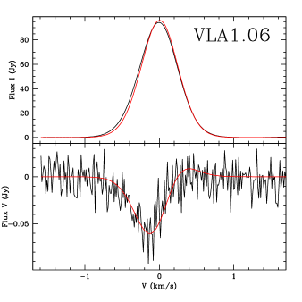
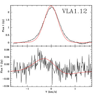
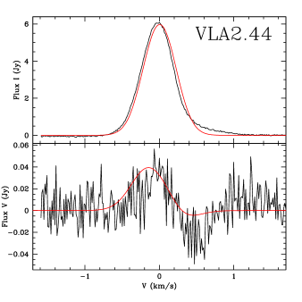
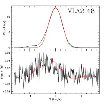
Figure 3: Total intensity spectra (I, upper panel) and circular polarization intensity spectra (V, lower panel) for the H₂O masers VLA1.06, VLA1.12, VLA2.44, and VLA2.48 (see Tables 4 and 5). The thick red line is the best-fit models of I and V emission obtained using the full radiative transfer method code for 22 GHz H₂O masers. The maser features were centered on zero velocity.

The H₂O masers in VLA 1 are distributed along the radio jet as previously observed by T03 (epoch 1999.25), S11 (epoch 2005.89), and K13 (epoch 2007.41). Surcis et al. (sur11 (2011)) found the H₂O masers clustered in three groups, named A, B, and C. In this work (epoch 2012.54), we detected 38 H₂O masers (named VLA1.01 – VLA1.38; Table 4, online material) in groups B and C, but not in A (Fig. 1). Group A was also not detected in 1999 and 2007. For a detailed comparison of the H₂O maser parameters measured in epochs 2005.89 and 2012.54 see Table 6 (online material).
We detected linearly polarized emission from seven H₂O masers ($P_{\rm{l}}=0.6\%-4.5\%$), and the error-weighted linear polarization angle is $\langle\chi\rangle_{\rm{VLA1}}=-41^{\circ}\pm 15^{\circ}$. The FRTM code was able to fit four out of the seven H₂O masers (Table 4). Because the lower limit of the fitting range of $T_{\rm{b}}\Delta\Omega$ is $10^{6}\leavevmode\nobreak\ \rm{K\leavevmode\nobreak\ sr}$, the estimated values of $\Delta V_{\rm{i}}$ and $T_{\rm{b}}\Delta\Omega$ are upper limits. The error-weighted values of the outputs are $\langle\Delta V_{\rm{i}}\rangle_{\rm{VLA1}}<2.4$ km s^-1, $\langle T_{\rm{b}}\Delta\Omega\rangle_{\rm{VLA1}}<10^{6}$ K sr, and $\langle\theta\rangle_{\rm{VLA1}}=+90$^∘${}^{+10^{\circ}}_{-10^{\circ}}$. This implies that the magnetic field is perpendicular to the linear polarization vectors and the error-weighted orientation on the plane of the sky is $\langle\Phi_{\rm{B}}\rangle_{\rm{VLA1}}=+49^{\circ}\pm 15$^∘. The foreground, ambient, and internal Faraday rotations are small or negligible as shown by S11.
Circularly polarized emission is detected in VLA1.06 ($P_{\rm{V}}=0.07\%$) and VLA1.12 ($1.8\%$). Because the FRTM code was not able to determine $T_{\rm{b}}\Delta\Omega$ and $\Delta V_{\rm{i}}$ for VLA1.12, we considered the values of the closest maser VLA1.10 to produce the $I$ and $V$ models (Fig. 3, online material). The estimated magnetic field strengths along the line of sight ($B_{||}$) are +18 mG and -544 mG (a negative magnetic field strength indicates that the magnetic field is pointing towards the observer; otherwise away from the observer). The magnetic field strength $B$ is related to $B_{||}$ by $B_{||}=B\leavevmode\nobreak\ \rm{cos}\theta$ if $\theta\neq\pm 90$^∘. Because $\langle\theta\rangle_{\rm{VLA1}}={90^{\circ}}^{+10^{\circ}}_{-10^{\circ}}$, we can only provide a lower limit of $B$ for VLA 1 (Table 6).

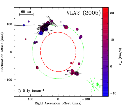
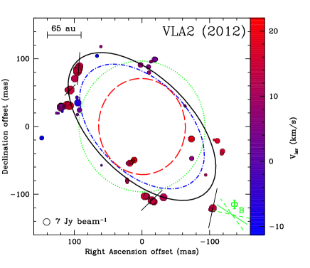
Figure 2: Comparison of the H₂O masers around VLA 2 in epoch 2005.89 (left panel; S11) and in epoch 2012.54 (right panel; present work). A comparison of the elliptical fits of the H₂O maser distributions observed in the past 13 years is also shown (see Fig. 1 for more details). The maser LSR radial velocity bar on the right of both panels shows the same velocity range. Four ellipses are drawn, which are assumed to have the same center (the (0,0) reference position). They are the results of the best fit of the H₂O masers detected by T03 (epoch 1999.25; red dashed ellipse), S11 (epoch 2005.89; green dotted ellipse), K13 (epoch 2007.41; blue dot-dashed ellipse), and the present work (epoch 2012.54; black solid ellipse). Their parameters are listed in Table 3.

3.2 VLA 2

We detected 68 H₂O masers (named VLA2.01–VLA2.68; Table 5, online material) showing an elliptical distribution similar to that observed in epoch 2007.41 (K13). An elliptical fit reveals that the semi-major axis ($a$) and the semi-minor axis ($b$) are $136\pm 4$ mas and $73\pm 2$ mas, respectively, and the position angle is $\rm{PA}=45$^∘$\pm 2$^∘. The center of the ellipse is at the position $\rm{c_{\alpha}}=+593\pm 2$ mas, $\rm{c_{\delta}}=-690\pm 3$ mas with respect to VLA1.06. The eccentricity, $e=\sqrt{1-(b/a)^{2}}$, of the fitted ellipse is $0.84\pm 0.05$.
Five H₂O masers show linearly polarized emission ($P_{\rm{l}}=0.7\%-1.6\%$), and the error-weighted linear polarization angle is $\langle\chi\rangle_{\rm{VLA2}}=-33^{\circ}\pm 21^{\circ}$. The FRTM code was able to properly fit only VLA2.64 and the outputs are $\Delta V_{\rm{i}}$${}_{,\rm{VLA2}}=1.98$ km s^-1, $T_{\rm{b}}\Delta\Omega$${}_{\rm{VLA2}}=6\times 10^{8}$ K sr, and $\theta_{\rm{VLA2}}=+84$^∘${}^{+6^{\circ}}_{-10^{\circ}}$. This implies that the magnetic field is perpendicular to the linear polarization vectors and the error-weighted orientation on the plane of the sky is $\langle\Phi_{\rm{B}}\rangle_{\rm{VLA2}}=+57^{\circ}\pm 21$^∘.
Circularly polarized emission was detected towards two H₂O masers, namely VLA2.44 ($P_{\rm{V}}=0.7\%$) and VLA2.48 ($P_{\rm{V}}=0.4\%$). These masers do not show linear polarization and consequently no information on $\Delta V_{\rm{i}}$ and $T_{\rm{b}}\Delta\Omega$ is available. In order to measure the magnetic field strength, we decided to assign values to $\Delta V_{\rm{i}}$ and $T_{\rm{b}}\Delta\Omega$ that could produce the best $I$ and $V$ fitting models. These are $\Delta V_{\rm{i}}$$\leavevmode\nobreak\ =2.0$ km s^-1 for both masers, and $T_{\rm{b}}\Delta\Omega$$\leavevmode\nobreak\ =5\times 10^{9}$ K sr and $T_{\rm{b}}\Delta\Omega$$\leavevmode\nobreak\ =10^{9}$ K sr for VLA2.44 and VLA2.48, respectively. The goodness of the fit can be seen in Fig. 3. The estimated $B_{||}$ are -152 mG and -103 mG.

4 Discussion

4.1 The immutable VLA 1

The H₂O masers in VLA 1 show a linear distribution ($\rm{PA}\approx 43$^∘) persistent over 13 years. Nevertheless, there are minor differences compared to S11. Specifically, the flux density has generally decreased from 2005 to 2012 (Table 6). This may explain the disappearance of the masers of group A, which also had larger $V_{\rm{lsr}}$ than groups B and C and thus they were probably tracing an occasional fast ejection event ($V_{\rm{lsr}}^{\rm{VLA\,1}}=9$ km s^-1, Carrasco-González et al. gon10 (2010)). The inferred magnetic field in VLA 1 is along the radio jet and it is almost aligned with the large-scale CO-outflow ($\rm{PA_{out}}=66$^∘; Hunter et al. hun94 (1994)), as measured in 2005 (Table 6).
The stability of the maser and magnetic field distribution around VLA 1 might indicate a relatively evolved stage of this massive YSO in comparison with VLA 2 (see below).

Table 1: Comparison of the fitted parameters of the ellipses from K13 (1999.25, 2005.89, 2007.41) and the present work (2012.54).

(1)	(2)	(3)	(4)	(5)	(6)
Epoch	$a$	$b$	PA	$e$	Expansion Velocity
	(mas)	(mas)	(∘)		($\rm{mas\leavevmode\nobreak\ yr^{-1}}$)	(km s-1)
1999.25	$71\pm 1$	$64\pm 1$	$5\pm 3$	$0.43\pm 0.01$
2005.89	$97\pm 3$	$93\pm 2$	$15\pm 45$	$0.28\pm 0.02$	$3.9\pm 0.5$	$24\pm 3$
2007.41	$111\pm 1$	$68\pm 1$	$45\pm 1$	$0.79\pm 0.02$	$9.2\pm 2.0$	$57\pm 12$
2012.54	$136\pm 4$	$73\pm 2$	$45\pm 2$	$0.84\pm 0.05$	$4.9\pm 0.8$	$30\pm 5$
					$4.9\pm 0.3$	$30\pm 2$

4.2 The evolution of the expanding H₂O maser shell in VLA 2

Unlikely VLA 1, VLA 2 has shown remarkable evolution both in structure and magnetic field in the last decade, as probed by the H₂O masers mapped with VLBI at four different epochs. In all epochs, the H₂O masers have shown a different distribution around VLA 2, in size and/or shape, going from circular (T03, S11) to elliptical (K13, present work; Fig. 2 and Table 3).
In epoch 1999.25, the elliptical fit reveals that $a$ and $b$ have almost the same value ($e=0.43\pm 0.01$, Table 3) indicating that the H₂O masers are tracing an almost circular shell-like structure (T03). This shell is thought to be the signature of a shock caused by the expansion of a non-collimated outflow; T03 also measured the proper motion of the individual H₂O masers, concluding that they are moving outward from VLA 2 at $\sim 19$ km s^-1.
In epoch 2005.89, S11 found that the circular shell increased its size by about 30 mas, but it did not changed its shape significantly ($e=0.28\pm 0.02$). In about six years the circular shell expanded with a velocity of $24\pm 3$ km s^-1 that is consistent with the proper motions of the individual H₂O masers (T03). This suggests that the formation of an early non-collimated outflow from a massive YSO is observed at mas scale; S11 also determined that the magnetic field is of the order of $1-2$ G around VLA 2 and it is oriented along $a$.
After only two years from the observations of S11, K13 observed that the H₂O maser shell is still expanding, but along a more dominant axis with $\rm{PA}=+45$^∘$\pm 1$^∘ ($e=0.79\pm 0.02$). The increment of the ellipticity could be the sign of the launching of a collimated jet that overtakes the non-collimated outflow. Surprisingly, the shell is now aligned with both the thermal radio jet and the magnetic field in VLA 1.
Our observations of epoch 2012.54 show that the expansion of the shell still continues after five years and that its ellipticity has increased ($e=0.84\pm 0.02$). The position angle of our fit is equal to that determined by K13 indicating that the supposed launching of a collimated jet has actually happened (Table 3).
In contrast to the magnetic field in VLA 1, the magnetic field in VLA 2 has changed its orientation substantially (Fig. 2). The magnetic field has rotated by about +40^∘ during the past seven years and it is now aligned with the major axis of the fitted ellipse of epoch 2012.54 ($\rm{PA}=+45$^∘$\pm 2$^∘). By comparing $\langle\Phi_{\rm{B}}\rangle_{\rm{VLA2}}$ with $\langle\Phi_{\rm{B}}\rangle_{\rm{VLA1}}$, we notice that the magnetic fields around VLA 2 and VLA 1 are now aligned with both the jet in VLA 1 and the elliptical H₂O maser shell in VLA 2. This configuration may arise if the large-scale magnetic field of W75N(B) drives the orientation of the two jets and potentially regulates HMSF as suggested by recent observations (Girart et al. gir09 (2009), Tan et al. tan13 (2013)). A test of this hypothesis may be to determine the morphology of the magnetic field of the region at large scale via dust polarization observations. Incidentally, we note that the inferred magnetic field direction also appears to be perpendicular to the filamentary core and its velocity gradient traced by NH₃ thermal emission (Carrasco-González et al. gon10 (2010)).
A possible physical framework to explain our results in VLA 2 may be provided by recent MHD simulations (Seifried et al. sei12 (2012)). In this context, the magnetic pressure drives a slow non-collimated outflow in the very first phase of protostellar formation. Immediately after the formation of a Keplerian disk, a short-lived fast and collimated jet overtakes the slow outflow. This could be qualitatively in agreement with our findings in VLA 2.
In addition, a comparison between $\overline{|B_{||}|}_{\rm{VLA2}}^{2005.89}$=345  mG and $\overline{|B_{||}|}_{\rm{VLA2}}^{2012.54}$=128  mG shows that the magnetic field in epoch 2012.54 is one third of the magnetic field measured in epoch 2005.89. The masers at the two epochs probe different gas properties and the measured variation of the magnetic field could simply be a consequence of it. We thus speculate that the variation may be due to the launching of the fast jet, but present simulations do not include the variation of the magnetic field strength during the early outflow evolution to corroborate our hypothesis.
From an observational perspective, to confirm our scenario it is necessary to monitor the expanding motion of the 22 GHz H₂O maser structure and the magnetic field evolution in the region over time. Furthermore, the determination of the 3D velocity structure of the outflow obtained with new proper motion measurements of the H₂O masers and of the evolution of the continuum morphology of VLA 2 will likewise be important.

5 Conclusions

We observed the massive star-forming region W75N(B) with the VLBA to detect linearly and circularly polarized emission from 22 GHz H₂O masers associated with the two radio sources VLA 1 and VLA 2. We observed that while the H₂O maser distribution and the magnetic field around VLA 1 have not changed since 2005, the shell structure of the masers around VLA 2 is still expanding and increasing its ellipticity. Furthermore, the magnetic field around VLA 2 has changed its orientation according to the new direction of the major-axis of the shell-like structure and it is now aligned with the magnetic field in VLA 1. We conclude that the H₂O masers around VLA 2 are tracing the evolution from a non-collimated to a collimated outflow.

Appendix A Tables

In Tables 4 and 5 we list all the H₂O maser features detected towards the two YSOs, VLA 1 and VLA 2, respectively. The tables are organized as follows. The name of the feature is reported in Col. 1. The positions, Cols. 2 and 3, refer to the brightest H₂O maser feature VLA1.06 that was used to self-calibrate the data. We estimated the absolute position of VLA1.06 to be $\alpha_{2000}=20^{\rm{h}}38^{\rm{m}}36^{\rm{s}}\!.435$ and $\delta_{2000}=42^{\circ}37^{\prime}34^{\prime\prime}\!\!.84$ (see Sect. 2). The peak flux density (I), the LSR velocity ($V_{\rm{lsr}}$), and the FWHM ($\Delta v\rm{{}_{L}}$) of the total intensity spectra of the maser features are reported in Cols. 4, 5, and 6, respectively; I, $V_{\rm{lsr}}$, and $\Delta v\rm{{}_{L}}$ are obtained using a Gaussian fit. The mean linear polarization fraction ($P_{\rm{l}}$) and the mean linear polarization angles ($\chi$) are instead reported in Cols. 8 and 9, respectively. We determined $P_{\rm{l}}$ and $\chi$ of each H₂O maser feature by only considering the consecutive channels (more than two) across the total intensity spectrum for which the polarized intensity is $\geq 5\sigma$.
In Cols. 9 and 10 are reported the values of the product of the brightness temperature $T_{\rm{b}}$ of the continuum radiation that is incident onto the masing region and the solid angle of the maser beam $\Delta\Omega$, which is known as the emerging brightness temperature $T_{\rm{b}}\Delta\Omega$, and the intrinsic thermal linewidth of the maser $\Delta V_{\rm{i}}$. Their values listed in the tables are the outputs of the FRTM code (Vlemmings et al. vle06 (2006)) that is based on the model for 22 GHz H₂O maser of Nedoluha & Watson (ned92 (1992)), for which the shapes of the total intensity, linear polarization, and circular polarization spectra depend on $T_{\rm{b}}\Delta\Omega$ and $\Delta V_{\rm{i}}$ (Nedoluha & Watson ned91 (1991, 1992)). We model the observed linear polarized and total intensity maser spectra by gridding $\Delta V_{i}$ between 0.4 km s^-1and 4.0 km s^-1, in steps of 0.025 km s^-1, using a least-squares fitting routine ($\chi^{2}$-model) with $10^{6}$ K sr $<T_{\rm{b}}\Delta\Omega<10^{11}$ K sr. We also set in our fit $(\Gamma+\Gamma_{\nu})=1\rm{s^{-1}}$, where $\Gamma$ is the maser decay rate and $\Gamma_{\nu}$ is the cross-relaxation rate for the magnetic substated (see Vlemmings et al. vle06 (2006) and S11 for more details).
From the maser theory we know that $P_{\rm{l}}$ of the H₂O maser emission depends on the degree of its saturation and the angle between the maser propagation direction and the magnetic field ($\theta$; e.g., Goldreich et al. gol73 (1973)). Because $T_{\rm{b}}\Delta\Omega$ determines the relation between $P_{\rm{l}}$ and $\theta$, from the outputs of the FRTM code we are able to estimate the angles $\theta$ that are reported in Col. 13. The errors of $T_{\rm{b}}\Delta\Omega$, $\Delta V_{\rm{i}}$, and $\theta$ are determined by analyzing the full probability distribution function.
Finally, the best estimates of $T_{\rm{b}}\Delta\Omega$ and $\Delta V_{\rm{i}}$ are then included in the FRTM code to produce the I and V models that are used for fitting the total intensity and circular polarized spectra of the H₂O masers (see Fig. 3). The magnetic field strength along the line of sight, which is reported in Col. 12, is finally evaluated by using the equation

$$B_{||}=B\leavevmode\nobreak\ cos\theta=\frac{P_{V}\leavevmode\nobreak\ \Delta v_{L}}{2\cdot A_{F-F^{\prime}}},$$ (1)

where $\Delta v_{L}$ is the FWHM of the total intensity spectrum, $P_{\rm{V}}=(V_{\rm{max}}-V_{\rm{max}})/I_{\rm{max}}$ is the circular polarization fraction (Col. 11), and the $A_{\rm{F-F^{\prime}}}$ coefficient, which depends on $T_{\rm{b}}\Delta\Omega$, describes the relation between the circular polarization and the magnetic field strength for a transition between a high ($F$) and low ($F^{\prime}$) rotational energy level (Vlemmings et al. vle06 (2006)).
In Table 6 we compare the parameters of the 22 GHz H₂O masers detected around VLA 1 and VLA 2 in epochs 2005.89 and 2012.54. The first three rows are the observed parameters. In Rows 4 and 5 are reported the measured linear ($P_{\rm{l}}$) and circular polarization fraction ($P_{\rm{V}}$) in percentage. In the rest of the table we compare the intrinsic charateristics of the masers and the magnetic field properties that have all been estimated from the outputs of the FRTM code.

Table 2: All 22 GHz H₂O maser features detected around VLA 1 (epoch 2012.54).

(1)	(2)	(3)	(4)	(5)	(6)	(7)	(8)	(9)	(10)	(11)	(12)	(13)
Maser	RA	Dec	Peak flux	$V_{\rm{lsr}}$	$\Delta v\rm{{}_{L}}$	$P_{\rm{l}}$	$\chi$	$\Delta V_{\rm{i}}$	$T_{\rm{b}}\Delta\Omega$	$P_{\rm{V}}$	$B_{||}$	$\theta$
	offset	offset	Density(I)
	(mas)	(mas)	(Jy/beam)	(km/s)	(km/s)	(%)	(∘)	(km/s)	(log K sr)	($\%$)	(mG)	(∘)
VLA1.01	-101.297	-188.122	$1.64\pm 0.16$	12.386	$0.47$	$-$	$-$	$-$	$-$	$-$	$-$	$-$
VLA1.02	-99.150	-191.898	$1.38\pm 0.17$	12.305	$0.44$	$-$	$-$	$-$	$-$	$-$	$-$	$-$
VLA1.03	-62.311	-218.605	$2.85\pm 0.12$	12.305	$0.44$	$-$	$-$	$-$	$-$	$-$	$-$	$-$
VLA1.04	-50.775	-176.990	$0.69\pm 0.04$	11.861	$0.42$	$-$	$-$	$-$	$-$	$-$	$-$	$-$
VLA1.05	-11.662	-39.768	$9.80\pm 0.04$	11.928	$0.53$	$0.9\pm 0.1$	$-30\pm 5$	$-$	$-$	$-$	$-$	$-$
VLA1.06	0	0	$94.32\pm 0.11$	10.593	$0.60$	$1.5\pm 0.4$	$-26\pm 6$	$<2.0$	$<6.00$	$0.07$	$+18\pm 6$	$90^{+7}_{-7}$
VLA1.07	18.020	-66.166	$2.19\pm 0.06$	9.501	$0.51$	$2.8\pm 0.3$	$-25\pm 8$	$<1.2$	$<6.00$	$-$	$-$	$90^{+29}_{-29}$
VLA1.08	19.114	-66.052	$1.27\pm 0.03$	9.811	$0.69$	$-$	$-$	$-$	$-$	$-$	$-$	$-$
VLA1.09	19.493	-64.823	$0.83\pm 0.03$	9.811	$0.52$	$-$	$-$	$-$	$-$	$-$	$-$	$-$
VLA1.10	23.998	18.848	$4.82\pm 0.06$	10.957	$0.77$	$2.8\pm 0.2$	$-52\pm 4$	$<2.4$	$<6.00$	$-$	$-$	$90^{+8}_{-8}$
VLA1.11	24.335	17.906	$1.68\pm 0.05$	11.820	$0.65$	$-$	$-$	$-$	$-$	$-$	$-$	$-$
VLA1.12	30.313	18.917	$2.33\pm 0.06$	11.159	$0.74$	$4.5\pm 1.4$	$-70\pm 7$	$-$	$-$	$1.8$	$-544\pm 272$	$-$
VLA1.13	31.787	-61.127	$2.50\pm 0.06$	12.872	$1.06$	$-$	$-$	$-$	$-$	$-$	$-$	$-$
VLA1.14	32.040	-61.161	$1.01\pm 0.04$	13.977	$1.14$	$-$	$-$	$-$	$-$	$-$	$-$	$-$
VLA1.15	32.166	19.795	$1.28\pm 0.06$	10.930	$0.70$	$-$	$-$	$-$	$-$	$-$	$-$	$-$
VLA1.16	36.587	11.280	$0.90\pm 0.07$	14.611	$1.05$	$-$	$-$	$-$	$-$	$-$	$-$	$-$
VLA1.17	36.671	-133.79	$1.10\pm 0.03$	9.784	$0.34$	$-$	$-$	$-$	$-$	$-$	$-$	$-$
VLA1.18	42.776	22.419	$1.07\pm 0.06$	11.267	$0.64$	$-$	$-$	$-$	$-$	$-$	$-$	$-$
VLA1.19	43.449	22.812	$1.08\pm 0.05$	11.362	$0.93$	$-$	$-$	$-$	$-$	$-$	$-$	$-$
VLA1.20	57.385	35.961	$3.95\pm 0.03$	8.652	$0.78$	$-$	$-$	$-$	$-$	$-$	$-$	$-$
VLA1.21	62.311	36.697	$0.81\pm 0.05$	11.389	$1.01$	$-$	$-$	$-$	$-$	$-$	$-$	$-$
VLA1.22	63.406	40.180	$4.27\pm 0.03$	9.933	$0.63$	$-$	$-$	$-$	$-$	$-$	$-$	$-$
VLA1.23	79.615	48.130	$16.48\pm 0.06$	12.845	$1.77$	$0.6\pm 0.1$	$-38\pm 5$	$-$	$-$	$-$	$-$	$-$
VLA1.24	80.836	49.847	$10.09\pm 0.07$	12.764	$1.16$	$0.8\pm 0.1$	$-40\pm 6$	$<3.6$	$<6.00$	$-$	$-$	$90^{+8}_{-8}$
VLA1.25	81.131	45.647	$1.52\pm 0.05$	11.267	$0.78$	$-$	$-$	$-$	$-$	$-$	$-$	$-$
VLA1.26	81.299	49.385	$7.80\pm 0.04$	13.640	$2.10$	$-$	$-$	$-$	$-$	$-$	$-$	$-$
VLA1.27	82.141	49.545	$1.93\pm 0.12$	15.703	$0.87$	$-$	$-$	$-$	$-$	$-$	$-$	$-$
VLA1.28	82.520	46.993	$1.22\pm 0.05$	11.348	$1.60$	$-$	$-$	$-$	$-$	$-$	$-$	$-$
VLA1.29	82.562	46.635	$1.65\pm 0.22$	15.298	$1.75$	$-$	$-$	$-$	$-$	$-$	$-$	$-$
VLA1.30	83.194	47.424	$0.45\pm 0.04$	10.148	$1.47$	$-$	$-$	$-$	$-$	$-$	$-$	$-$
VLA1.31	88.246	19.569	$4.00\pm 0.09$	9.407	$1.53$	$-$	$-$	$-$	$-$	$-$	$-$	$-$
VLA1.32	89.383	18.864	$4.61\pm 0.05$	11.038	$2.66$	$-$	$-$	$-$	$-$	$-$	$-$	$-$
VLA1.33	89.719	19.123	$3.97\pm 0.13$	12.494	$1.64$	$-$	$-$	$-$	$-$	$-$	$-$	$-$
VLA1.34	89.762	21.153	$1.72\pm 0.08$	12.090	$1.99$	$-$	$-$	$-$	$-$	$-$	$-$	$-$
VLA1.35	89.804	19.898	$4.58\pm 0.04$	13.317	$0.78$	$-$	$-$	$-$	$-$	$-$	$-$	$-$
VLA1.36	90.140	19.264	$2.24\pm 0.09$	10.391	$3.80$	$-$	$-$	$-$	$-$	$-$	$-$	$-$
VLA1.37	91.109	16.884	$1.67\pm 0.05$	14.018	$0.92$	$-$	$-$	$-$	$-$	$-$	$-$	$-$
VLA1.38	94.098	8.427	$0.61\pm 0.05$	11.537	$1.21$	$-$	$-$	$-$	$-$	$-$	$-$	$-$

Table 3: All 22 GHz H₂O maser features detected around VLA 2 (epoch 2012.54).

(1)	(2)	(3)	(4)	(5)	(6)	(7)	(8)	(9)	(10)	(11)	(12)	(13)
Maser	RA	Dec	Peak flux	$V_{\rm{lsr}}$	$\Delta v\rm{{}_{L}}$	$P_{\rm{l}}$	$\chi$	$\Delta V_{\rm{i}}$	$T_{\rm{b}}\Delta\Omega$	$P_{\rm{V}}$	$B_{||}$	$\theta$
	offset	offset	Density(I)
	(mas)	(mas)	(Jy/beam)	(km/s)	(km/s)	(%)	(∘)	(km/s)	(log K sr)	($\%$)	(mG)	(∘)
VLA2.01	473.816	-727.013	$1.24\pm 0.05$	16.309	$0.54$	$-$	$-$	$-$	$-$	$-$	$-$	$-$
VLA2.02	474.784	-730.545	$0.48\pm 0.03$	16.512	$0.73$	$-$	$-$	$-$	$-$	$-$	$-$	$-$
VLA2.03	481.352	-711.754	$1.20\pm 0.03$	16.498	$0.79$	$-$	$-$	$-$	$-$	$-$	$-$	$-$
VLA2.04	485.984	-710.171	$0.22\pm 0.02$	20.044	$0.64$	$-$	$-$	$-$	$-$	$-$	$-$	$-$
VLA2.05	487.962	-811.104	$6.62\pm 0.04$	14.233	$0.43$	$1.6\pm 0.1$	$-12\pm 4$	$-$	$-$	$-$	$-$	$-$
VLA2.06	491.709	-813.095	$0.57\pm 0.04$	13.384	$0.53$	$-$	$-$	$-$	$-$	$-$	$-$	$-$
VLA2.07	498.530	-761.936	$0.35\pm 0.03$	11.982	$0.73$	$-$	$-$	$-$	$-$	$-$	$-$	$-$
VLA2.08	519.370	-737.568	$0.97\pm 0.02$	6.670	$0.72$	$-$	$-$	$-$	$-$	$-$	$-$	$-$
VLA2.09	519.539	-707.607	$0.69\pm 0.02$	18.898	$0.79$	$-$	$-$	$-$	$-$	$-$	$-$	$-$
VLA2.10	519.749	-708.904	$3.24\pm 0.02$	18.588	$0.56$	$-$	$-$	$-$	$-$	$-$	$-$	$-$
VLA2.11	528.507	-660.904	$0.21\pm 0.02$	2.369	$0.55$	$-$	$-$	$-$	$-$	$-$	$-$	$-$
VLA2.12	529.643	-659.538	$0.22\pm 0.02$	2.504	$0.57$	$-$	$-$	$-$	$-$	$-$	$-$	$-$
VLA2.13	560.883	-794.949	$6.01\pm 0.03$	11.645	$0.53$	$-$	$-$	$-$	$-$	$-$	$-$	$-$
VLA2.14	572.629	-591.267	$0.84\pm 0.02$	3.798	$0.66$	$-$	$-$	$-$	$-$	$-$	$-$	$-$
VLA2.15	574.061	-591.526	$1.03\pm 0.02$	4.648	$0.57$	$-$	$-$	$-$	$-$	$-$	$-$	$-$
VLA2.16	574.945	-801.651	$3.76\pm 0.18$	15.110	$0.64$	$-$	$-$	$-$	$-$	$-$	$-$	$-$
VLA2.17	575.871	-800.690	$3.02\pm 0.12$	15.420	$1.05$	$-$	$-$	$-$	$-$	$-$	$-$	$-$
VLA2.18	576.250	-800.716	$2.16\pm 0.15$	14.988	$1.24$	$-$	$-$	$-$	$-$	$-$	$-$	$-$
VLA2.19	578.397	-799.526	$8.05\pm 0.05$	14.409	$0.62$	$1.1\pm 0.1$	$-46\pm 5$	$-$	$-$	$-$	$-$	$-$
VLA2.20	578.945	-594.635	$0.32\pm 0.03$	6.158	$0.62$	$-$	$-$	$-$	$-$	$-$	$-$	$-$
VLA2.21	579.829	-796.158	$0.27\pm 0.03$	17.334	$1.10$	$-$	$-$	$-$	$-$	$-$	$-$	$-$
VLA2.22	580.039	-594.902	$0.29\pm 0.03$	6.104	$0.60$	$-$	$-$	$-$	$-$	$-$	$-$	$-$
VLA2.23	582.313	-610.703	$0.60\pm 0.02$	7.776	$0.54$	$-$	$-$	$-$	$-$	$-$	$-$	$-$
VLA2.24	583.197	-602.474	$1.14\pm 0.02$	4.648	$0.57$	$-$	$-$	$-$	$-$	$-$	$-$	$-$
VLA2.25	585.555	-793.598	$2.79\pm 0.13$	14.867	$1.10$	$-$	$-$	$-$	$-$	$-$	$-$	$-$
VLA2.26	586.481	-793.186	$1.75\pm 0.03$	13.613	$1.22$	$-$	$-$	$-$	$-$	$-$	$-$	$-$
VLA2.27	588.755	-793.449	$6.04\pm 0.15$	15.298	$0.84$	$-$	$-$	$-$	$-$	$-$	$-$	$-$
VLA2.28	594.817	-599.632	$1.52\pm 0.02$	7.371	$0.58$	$-$	$-$	$-$	$-$	$-$	$-$	$-$
VLA2.29	602.522	-739.132	$0.26\pm 0.02$	22.039	$0.89$	$-$	$-$	$-$	$-$	$-$	$-$	$-$
VLA2.30	604.205	-740.036	$2.84\pm 0.02$	20.758	$0.71$	$-$	$-$	$-$	$-$	$-$	$-$	$-$
VLA2.31	606.016	-740.799	$0.44\pm 0.02$	18.696	$1.20$	$-$	$-$	$-$	$-$	$-$	$-$	$-$
VLA2.32	607.153	-741.844	$0.71\pm 0.02$	19.316	$0.81$	$-$	$-$	$-$	$-$	$-$	$-$	$-$
VLA2.33	608.079	-742.798	$0.73\pm 0.02$	19.248	$1.35$	$-$	$-$	$-$	$-$	$-$	$-$	$-$
VLA2.34	608.416	-743.553	$0.91\pm 0.02$	19.976	$0.92$	$-$	$-$	$-$	$-$	$-$	$-$	$-$
VLA2.35	610.732	-744.667	$3.19\pm 0.02$	18.494	$0.75$	$-$	$-$	$-$	$-$	$-$	$-$	$-$
VLA2.36	613.847	-744.747	$0.48\pm 0.05$	10.984	$0.87$	$-$	$-$	$-$	$-$	$-$	$-$	$-$
VLA2.37	614.605	-770.691	$0.64\pm 0.04$	13.249	$0.72$	$-$	$-$	$-$	$-$	$-$	$-$	$-$
VLA2.38	614.647	-772.896	$0.35\pm 0.03$	13.573	$0.79$	$-$	$-$	$-$	$-$	$-$	$-$	$-$
VLA2.39	614.774	-768.429	$0.34\pm 0.04$	12.535	$0.90$	$-$	$-$	$-$	$-$	$-$	$-$	$-$
VLA2.40	652.539	-747.784	$0.24\pm 0.02$	-2.191	$0.90$	$-$	$-$	$-$	$-$	$-$	$-$	$-$
VLA2.41	653.465	-572.544	$0.29\pm 0.02$	7.506	$1.00$	$-$	$-$	$-$	$-$	$-$	$-$	$-$
VLA2.42	659.149	-586.201	$0.44\pm 0.02$	-10.155	$0.75$	$-$	$-$	$-$	$-$	$-$	$-$	$-$
VLA2.43	685.042	-666.283	$1.08\pm 0.02$	2.329	$1.09$	$-$	$-$	$-$	$-$	$-$	$-$	$-$
VLA2.44	685.084	-601.471	$6.08\pm 0.14$	14.934	$0.52$	$-$	$-$	$-$	$-$	$0.7$	$-152\pm 73$	$-$
VLA2.45	686.305	-605.049	$8.87\pm 0.14$	15.325	$0.49$	$1.2\pm 0.2$	$-4\pm 7$	$-$	$-$	$-$	$-$	$-$
VLA2.46	687.610	-655.483	$4.26\pm 0.02$	-6.636	$0.64$	$-$	$-$	$-$	$-$	$-$	$-$	$-$
VLA2.47	687.947	-606.522	$13.84\pm 0.15$	15.285	$0.44$	$-$	$-$	$-$	$-$	$-$	$-$	$-$
VLA2.48	688.157	-609.310	$12.97\pm 0.07$	16.094	$0.60$	$-$	$-$	$-$	$-$	$0.4$	$-103\pm 43$	$-$
VLA2.49	688.199	-672.810	$0.27\pm 0.02$	1.776	$0.63$	$-$	$-$	$-$	$-$	$-$	$-$	$-$
VLA2.50	688.831	-647.507	$0.38\pm 0.02$	-3.158	$0.56$	$-$	$-$	$-$	$-$	$-$	$-$	$-$
VLA2.51	692.115	-619.831	$4.77\pm 0.04$	12.777	$0.52$	$-$	$-$	$-$	$-$	$-$	$-$	$-$
VLA2.52	699.188	-636.635	$14.07\pm 0.17$	15.002	$0.59$	$0.7\pm 0.1$	$-45\pm 6$	$-$	$-$	$-$	$-$	$-$
VLA2.53	699.609	-659.790	$9.75\pm 0.03$	17.213	$0.58$	$-$	$-$	$-$	$-$	$-$	$-$	$-$
VLA2.54	702.514	-655.918	$0.65\pm 0.04$	16.256	$0.55$	$-$	$-$	$-$	$-$	$-$	$-$	$-$
VLA2.55	702.809	-657.299	$1.11\pm 0.05$	16.269	$0.46$	$-$	$-$	$-$	$-$	$-$	$-$	$-$
VLA2.56	703.398	-636.490	$1.16\pm 0.06$	14.584	$0.42$	$-$	$-$	$-$	$-$	$-$	$-$	$-$
VLA2.57	703.483	-658.810	$9.30\pm 0.07$	15.851	$0.46$	$-$	$-$	$-$	$-$	$-$	$-$	$-$
VLA2.58	710.514	-668.293	$0.26\pm 0.02$	-6.219	$0.65$	$-$	$-$	$-$	$-$	$-$	$-$	$-$
VLA2.59	710.556	-926.731	$4.29\pm 0.03$	8.179	$0.72$	$-$	$-$	$-$	$-$	$-$	$-$	$-$
VLA2.60	711.987	-661.125	$3.56\pm 0.02$	6.764	$1.09$	$-$	$-$	$-$	$-$	$-$	$-$	$-$
VLA2.61	712.282	-660.404	$1.14\pm 0.02$	8.180	$0.88$	$-$	$-$	$-$	$-$	$-$	$-$	$-$
VLA2.62	712.282	-658.833	$0.88\pm 0.06$	10.243	$0.62$	$-$	$-$	$-$	$-$	$-$	$-$	$-$
VLA2.63	712.450	-661.923	$10.81\pm 0.03$	5.929	$0.83$	$-$	$-$	$-$	$-$	$-$	$-$	$-$
VLA2.64	714.597	-925.274	$26.25\pm 0.04$	9.232	$0.53$	$0.7\pm 0.1$	$-48\pm 3$	$1.98^{+0.05}_{-0.17}$	$8.8^{+0.3}_{-0.1}$	$-$	$-$	$84^{+6}_{-10}$
VLA2.65	716.071	-671.002	$0.19\pm 0.02$	-7.449	$0.89$	$-$	$-$	$-$	$-$	$-$	$-$	$-$
VLA2.66	719.018	-670.666	$0.26\pm 0.02$	5.308	$0.79$	$-$	$-$	$-$	$-$	$-$	$-$	$-$
VLA2.67	740.785	-707.310	$0.90\pm 0.02$	-11.193	$0.59$	$-$	$-$	$-$	$-$	$-$	$-$	$-$
VLA2.68	742.258	-708.374	$0.24\pm 0.02$	-11.166	$0.51$	$-$	$-$	$-$	$-$	$-$	$-$	$-$

Table 4: Comparison of 22 GHz H₂O maser parameters between epochs 2005.89 (S11) and 2012.54 (this work).

	epoch 2005.89		epoch 2012.54
	VLA 1	VLA 2	VLA 1	VLA 2
Number of maser features	36	88	38	68
$V_{\rm{lsr}}$ range (km s-1)	$[+8.1;+24.7]$	$[-7.7;+14.8]$	$[+9.4;+15.7]$	$[-11.2;+22.0]$
$I$ range (Jy beam-1)	$[0.13;158.28]$	$[0.09;198.45]$	$[0.45;94.32]$	$[0.19;26.25]$
	Polarization
$P_{\rm{l}}$ range (%)	$[0.6;25.7]$	$[0.2;6.1]$	$[0.6;4.5]$	$[0.7;1.6]$
$P_{\rm{V}}$ range (%)	$[0.3;4.2]$	$[0.1;3.0]$	$[0.1;1.8]$	$[0.4;0.7]$
	Intrinsic characteristics
$\Delta V_{\rm{i}}$ range (km s-1)	$[0.6;2.0]$	$[0.7;3.4]$	$[1.2;3.6]$	2.0
$T_{\rm{b}}\Delta\Omega$ range (log K sr)	$[8.9;10.7]$	$[8.6;10.7]$	$[6.0;6.0]$	8.8
$\langle\Delta V_{\rm{i}}\rangle$ (km s-1)	$1.0^{+0.8}_{-0.2}$	$2.5^{+0.6}_{-0.4}$	$<2.4$	$2.0^{+0.1}_{-0.2}$
$\langle T_{\rm{b}}\Delta\Omega\rangle$ (log K sr)	$10.6^{+1.1}_{-0.5}$	$9.4^{+0.6}_{-0.9}$	$<6.0$	$8.8^{+0.3}_{-0.1}$
$T$ (K)	$400$	$2500$	$<2300$	$1600$
$\Gamma+\Gamma_{\nu}$	$3$	$14$	$<13$	$9$
	Magnetic field
$\chi$ range (∘)	$[-90;+58]$	$[-90;+83]$	$[-70;-25]$	$[-48;-4]$
$\theta$ range (∘)	$[+66;+90]$	$[+61;+90]$	$[+90;+90]$	$+84$
$\Phi_{\rm{B}}$ range (∘)	$[-32;0]$	$[-7;0]$	$[+20;+65]$	$[+42;+86]$
$|B_{||}|$ range (mG)	$[54;809]$	$[38;957]$	$[18;544]$	$[103;152]$
$\langle\chi\rangle$ (∘)	$-67\pm 40$	$-72\pm 32$	$-41\pm 15$	$-33\pm 21$
$\langle\theta\rangle$ (∘)	$+83^{+7}_{-15}$	$+85^{+6}_{-36}$	$+90^{+10}_{-10}$	$+84^{+6}_{-10}$
$\langle\Phi_{\rm{B}}\rangle$ (∘)	$+23\pm 40$	$+18\pm 32$	$+49\pm 15$	$+57\pm 21$
$\langle|B_{||}|\rangle$ (mG)	$81\pm 62$	$145\pm 110$	$>18$	$116\pm 35$
$\langle|B|\rangle$ (mG)	$665\pm 509$	$1663\pm 1262$	$>104$	$1110\pm 335$
Arithmetic mean of $|B_{||}|$ (mG)	$264$	$345$	$281$	$128$