Locally tunable disorder and entanglement
in the one-dimensional plaquette orbital model

Abstract

We introduce a one-dimensional plaquette orbital model with a topology of a ladder and alternating interactions between $x$ and $z$ pseudospin components along both the ladder legs and on the rungs. We show that it is equivalent to an effective spin model in a magnetic field, with spin dimers that replace plaquettes and are coupled along the chain by three-spin interactions. Using perturbative treatment and mean field approaches with dimer correlations we study the ground state spin configuration and its defects in the lowest excited states. By the exact diagonalization approach we find that the quantum effects in the model are purely short-range and we get estimated values of the ground state energy and the gap in the thermodynamic limit from the system sizes up to $L=12$ dimers. Finally, we study a class of excited states with classical-like defects accumulated in the central region of the chain to find that in this region the quantum entanglement measured by the mutual information of neighboring dimers is locally increased and coincides with disorder and frustration. Such islands of entanglement in otherwise rather classical system may be of interest in the context of quantum computing devices.

I Introduction

Transition-metal oxides with active orbital degrees of freedom are frequently described in terms of spin-orbital models Tokura ; Hfm ; Ole05 ; Kha05 ; Ole12 which are realizations of the early idea of Kugel and Khomskii Kug82 that orbital operators have to be treated with their full dynamics in the limit of large on-site Coulomb interactions. The interplay between spin and orbital (pseudospin) interactions on superexchange bonds follows from the mechanism of effective magnetic interactions at strong correlation and is responsible for numerous quantum properties which originate from spin-orbital entanglement Ole12 . This phenomenon is similar to entanglement in spin models Ami08 , but occurs here in a larger Hilbert space You12 and has measurable consequences at finite temperature as found, for instance, in the phase diagrams Hor08 and in ferromagnetic dimerized interactions Her11 in the vanadium perovskites. In higher dimensional systems exotic spin states are also triggered in the ground state by entangled spin-orbital interactions in certain situations, as in: (i) the $d^{1}$ spin-orbital model on the triangular lattice Cha11 , (ii) the two-dimensional (2D) Kugel-Khomskii model Brz12 , and (iii) spinel and pyrochlore crystals with active $t_{2g}$ orbitals Bat11 . Such entangled spin-orbital states are very challenging but also notoriously difficult to investigate except for a few exactly solvable 1D models Li98 ; Brz14 .

To avoid the difficulties caused by entanglement one considers frequently ferromagnetic systems, where orbital interactions alone are responsible for the nature of both the ground and excited states. Orbital interactions in Mott insulators depend on the type of active and partly filled $3d$ orbitals — they have distinct properties for either $e_{g}$ symmetry vdB99 ; vdB04 ; Fei05 ; Ryn10 , or $t_{2g}$ symmetry Dag08 ; Wro10 ; Tro13 ; Che13 . In contrast to spin models, their symmetry is lower than SU(2) due to directional character of orbital interactions which manifests itself in their intrinsic frustration. The models which focus on such frustrated interactions are the 2D compass model on the square lattice vdB13 ; Nus05 ; Dou05 ; Dor05 ; Tan07 ; Wen08 ; Orus09 ; Dus09 ; Cin10 ; Brz10 ; Tro10 , the exactly solvable 1D compass model Brz07 ; You14 , the compass ladder Brz09 and the Kitaev model on the honeycomb lattice Kit06 ; Bas07 . The former includes only two spin components and 1D order arises in the highly degenerate ground state Dou05 ; Dor05 ; Tan07 ; Wen08 which is robust with respect to perturbing Heisenberg interactions Tro10 , while the latter provides an exactly solvable case of a spin liquid with only nearest neighbor (NN) spin correlations.

The interest in the 2D compass model is motivated by new opportunities it provides for quantum computing Dou05 . This motivated also plaquette orbital model (POM) introduced for a square lattice by Wenzel and Janke Wen09 which exhibits orientational long-range order in its classical version Bis10 . Here we will focus on the 1D quantum version of the POM and investigate the nature of the ground state and of low energy excitations. The purpose of this paper is to highlight the importance of entangled states which lead to pronounced dimer correlations in the 1D POM which consists of repeated interactions of $x$ and $z$ pseudospin component along three bonds of a plaquette, called for this reason also the $Cx$-$Cz$ model. As we show below, this model has rather surprising properties which may be captured only in analytic methods which go beyond standard mean-field (MF) approaches.

The paper is organized as follows: In Sec. II we introduce the $Cx$-$Cz$ Hamiltonian and derive its block-diagonal form making use of its local symmetries. In Sec. III we present a perturbative approach to the model within its invariant subspaces up to third order for the ground-state energies. The approximate solutions of the model are presented in Sec. IV where we introduce a single-dimer MF approach and more general two-dimer and three-dimer MF approaches to show the ground state spin configuration in different subspaces being the lowest excited states of the model. In Sec. V the exact diagonalization results are shown for the maximal system size of $L=12$ dimers. Finally, in Sec. VI we present the summary and main conclusions. The paper is supplemented with two Appendices: (i) Appendix A showing the additional details on spin transformation used in Sec. II, and (ii) Appendix B showing the duality between the interaction and free terms in the block-diagonal $Cx$-$Cz$ Hamiltonian.

II Hamilonian and its symmetries

The Hamiltonian of the 1D POM ($Cx$-$Cz$ model) of $L$ sites can be written as follows,

$${\cal H} = \sum_{i=1}^{L}\left\{X_{i,1}X_{i,2}+X_{i,2}X_{i,3}+X_{i,3}X_{i,4}\right.$$ (1)

$$+ \left.Z_{i,1}Z_{i+1,2}+Z_{i,1}Z_{i,4}+Z_{i,4}Z_{i+1,3}\right\},$$

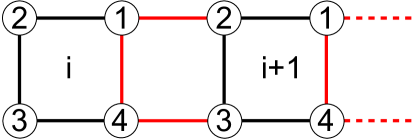
where $X_{i,p}$ and $Z_{i,p}$ are the $x$ and $z$ Pauli matrices at site $p$ of the plaquette $i$ — see Fig. 1. We assume periodic boundary conditions (PBCs) of the form $Z_{L+1,2}\equiv Z_{1,2}$ and $Z_{L+1,3}\equiv Z_{1,3}$. There are two types of the symmetry operators specific to the model, namely:

$$P_{i}^{z} = Z_{i,1}Z_{i,2}Z_{i,3}Z_{i,4},$$ (2)

$$P_{i}^{x} = X_{i+1,2}X_{i,1}X_{i,4}X_{i+1,3}.$$ (3)

In what follows we will make use of these symmetries to find a block-diagonal form of the Hamiltonian ${\cal H}$ by two consecutive spin transformation.

Figure 1: (Color online) Schematic view of the Hamiltonian of Eq. (1). Black (red) lines stand for the $XX$ ($ZZ$) bonds.

The key observation for Pauli matrices defined on a product space of a many-body system is that a product of $Z_{i,p}$ ($X_{i,p}$) operators over any subset of the system is another $z$ ($x$) Pauli operator. Of course, to transform all $Z_{i,p}$ ($X_{i,p}$) operators into new ones one has to choose these subsets carefully to keep track of the canonical commutation relations, saying that $z$ and $x$ Pauli operators having the same site index anticommute and otherwise commute. This we can assure by checking the intersections of the subsets over which the products are taken; if the intersection contains odd number of sites then the new $z$ and $x$ Pauli operators will anticommute, in opposite case they will commute. One can easily verify that these rules are satisfied by the transformation that we use to take care of the $P_{i}^{z}$ symmetries of Hamiltonian (2). The transformation is defined for each $X$-plaquette separately as,

$$X_{i,1} = \tilde{X}_{i,1},,$$

$$X_{i,2} = \tilde{X}_{i,1}\tilde{X}_{i,2},$$

$$X_{i,3} = \tilde{X}_{i,1}\tilde{X}_{i,2}\tilde{X}_{i,3},$$

$$X_{i,4} = \tilde{X}_{i,1}\tilde{X}_{i,2}\tilde{X}_{i,3}\tilde{X}_{i,4},$$ (4)

and

$$Z_{i,1} = \tilde{Z}_{i,1}\tilde{Z}_{i,2},$$

$$Z_{i,2} = \tilde{Z}_{i,2}\tilde{Z}_{i,3},$$

$$Z_{i,3} = \tilde{Z}_{i,3}\tilde{Z}_{i,4},$$

$$Z_{i,4} = \tilde{Z}_{i,4}.$$ (5)

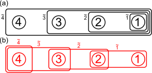
The operators $\tilde{X}{}_{i,p}$ and $\tilde{Z}_{i,p}$ are new $x$ and $z$ Pauli matrices satisfying all the canonical commutation relations and the tranformation is a bijection which means that the inverse transformation exists — its form can be easily guessed if we notice that, e.g. $\tilde{X}_{i,2}=X_{i,2}X_{i,1}$ and $\tilde{Z}_{i,3}=Z_{i,4}Z_{i,3}$. This of course exploits the fact that any Pauli matrix squared gives identity. The easiest way to verify that the transformations given by Eqs. (4) and (5) really map Pauli operators into other set of Pauli operators is by drawing — see Fig. 2.

Figure 2: (Color online) Schematic view of the transformations used for the OPM: (a) in Eqs. (4), and (b) in Eq. (5). Numbered circles symbolize otiginal Pauli matrices, $\left\{X_{i,1},X_{i,2},X_{i,3},X_{i,4}\right\}$ (black circles) or $\left\{Z_{i,1},Z_{i,2},Z_{i,3},Z_{i,4}\right\}$ (red circles). The frames labeled with tilded numbers symbolize new Pauli matrices, $\left\{\tilde{X}_{i,1},\tilde{X}_{i,2},\tilde{X}_{i,3},\tilde{X}_{i,4}\right\}$ (black frames), or $\left\{\tilde{Z}_{i,1},\tilde{Z}_{i,2},\tilde{Z}_{i,3},\tilde{Z}_{i,4}\right\}$ (red frames).

It is straightforward to get the Hamiltonian in terms of tilde operators, i.e.,

$${\cal H} = \sum_{i=1}^{L}\left\{\tilde{X}_{i,2}+\tilde{X}_{i,3}+\tilde{X}_{i,4}+r_{i}\tilde{Z}_{i,2}\tilde{Z}_{i+1,2}\tilde{Z}_{i+1,3}\right.$$ (6)

$$+ \left.r_{i}\tilde{Z}_{i,2}\tilde{Z}_{i,4}+\tilde{Z}_{i,4}\tilde{Z}_{i+1,3}\tilde{Z}_{i+1,4}\right\},$$

where $r_{i}=\pm 1$ are the eigenvalues of the symmetry operator $P_{i}^{z}=\tilde{Z}_{i,1}$, which we are allowed to insert for ${\cal H}$ does not depend on $\tilde{X}_{i,1}$. Consequently the $P_{i}^{x}$ symmetries transform as

$$P_{i}^{x}=X_{i+1,2}X_{i,1}X_{i,4}X_{i+1,3}=\tilde{X}_{i,2}\tilde{X}_{i,3}\tilde{X}_{i,4}\tilde{X}_{i+1,3}.$$ (7)

Now the hard part starts because this symmetry mixes the operators on neighboring plaquettes. How to guess next spin transformation that will make use of $P_{i}^{x}$ symmetries, provided that such a transformation exists? We can try to demand that in terms of new Pauli operators the symmetry transforms into a single Pauli operator, as it happened with $P_{i}^{z}$, i.e., $P_{i}^{x}=X^{\prime}_{i,4}$. This means that $X^{\prime}_{i,4}=\tilde{X}_{i,2}\tilde{X}_{i,3}\tilde{X}_{i,4}\tilde{X}_{i+1,3}$. The form of the transformation (4) suggests that the other $x$ operators can be constructed in the following way,

$$X^{\prime}_{i,2} = \tilde{X}_{i,2}\left(\tilde{X}_{i+1,3}\right),$$

$$X^{\prime}_{i,3} = \tilde{X}_{i,2}\tilde{X}_{i,3}\left(\tilde{X}_{i+1,3}\right),$$

$$X^{\prime}_{i,4} = \tilde{X}_{i,2}\tilde{X}_{i,3}\tilde{X}_{i,4}\left(\tilde{X}_{i+1,3}\right),$$ (8)

where the main difference with respect to Eq. (4) is that we keep the contribution from the neighboring plaquette (in bracket) for every $X^{\prime}_{i,p}$. By analogy to the transformation (5) we can also guess the form of the new $z$ operators,

$$Z^{\prime}_{i,2} = \tilde{Z}_{i,2}\tilde{Z}_{i,3}\left(\tilde{Z}_{i-1,2}\right),$$

$$Z^{\prime}_{i,3} = \tilde{Z}_{i,3}\tilde{Z}_{i,4}\left(\tilde{Z}_{i-1,2}\right),$$

$$Z^{\prime}_{i,4} = \tilde{Z}_{i,4}.$$ (9)

Again the difference is in terms in brackets coming from the neighboring plaquette - these were involved in Eq. (9) in such a way that the canonical commutation relations between primed Pauli operators are satisfied. Now to get the Hamiltonian in terms of new, primed operators we need to inverse the above transformations. This can be done in straightforward fashion and we arrive at,

$$\tilde{X}_{i,2} \!=\! X^{\prime}_{i,2}\left(\tilde{X}_{i+1,3}\right)=X^{\prime}_{i,2}\left(X^{\prime}_{i+1,2}X^{\prime}_{i+1,3}\right),$$

$$\tilde{X}_{i,3} \!=\! X^{\prime}_{i,2}X^{\prime}_{i,3},$$

$$\tilde{X}_{i,4} \!=\! X^{\prime}_{i,3}X^{\prime}_{i,4},$$ (10)

and

$$\tilde{Z}_{i,2} \!=\! Z^{\prime}_{i,2}Z^{\prime}_{i,3}Z^{\prime}_{i,4},$$

$$\tilde{Z}_{i,3} \!=\! Z^{\prime}_{i,3}Z^{\prime}_{i,4}\!\left(\tilde{Z}_{i-1,2}\right)\!=\!Z^{\prime}_{i,3}Z^{\prime}_{i,4}\left(Z^{\prime}_{i-1,2}Z^{\prime}_{i-1,3}Z^{\prime}_{i-1,4}\right),$$

$$\tilde{Z}_{i,4} \!=\! Z^{\prime}_{i,4}.$$ (11)

Quite miraculously these rather complicated formulas inserted into Hamiltonian (6) give a rather simple structure of the block-diagonal Hamiltonian,

$${\cal H} = \sum_{i=1}^{L}\left\{s_{i}X^{\prime}_{i,3}+X^{\prime}_{i,2}X^{\prime}_{i,3}+X^{\prime}_{i,2}X^{\prime}_{i+1,2}X^{\prime}_{i+1,3}\right.$$ (12)

$$+ \left.r_{i}Z^{\prime}_{i+1,2}+r_{i}Z^{\prime}_{i,2}Z^{\prime}_{i,3}+Z^{\prime}_{i+1,3}Z^{\prime}_{i,2}Z^{\prime}_{i,3}\right\},$$

where half of the initial spins are replaced by the quantum numbers $r_{i},s_{i}=\pm 1$ being the eigenvalues of the symmetry operators $P_{i}^{z}$ and $P_{i}^{x}$. Thus a spin model on a ladder show in Fig. 1 has become a model of a dimerized chain with two spins per unit cell, namely $Z^{\prime}_{i,2}$ and $Z^{\prime}_{i,3}$. Note that unlike in case of the 2D quantum compass model, where the similar spin transformations were used to obtain reduced Hamiltonian Brz10 , here the PBCs do not yield any non-local operators in ${\cal H}$ of Eq. (12). Here the PBCs assumed for the initial spins become PBCs for both tilde operators of Eq. (6) and primed ones of Eq. (12). Before discussing the reduced Hamiltonian in more details let us end this Section by a one more (simple!) spin transformation that puts ${\cal H}$ in more symmetric and convenient form, namely

$$\sigma_{i,3}^{x} = s_{i}X^{\prime}_{i,3},$$

$$\sigma_{i,2}^{x} = X^{\prime}_{i,2}X^{\prime}_{i,3},$$

$$\sigma_{i,3}^{z} = r_{i}Z^{\prime}_{i,2}Z^{\prime}_{i,3},$$

$$\sigma_{i,2}^{z} = r_{i-1}Z^{\prime}_{i,2},$$ (13)

which finally gives,

$${\cal H} = \sum_{i=1}^{L}\left\{\left(\sigma_{i,2}^{z}+\sigma_{i,3}^{z}\right)+\left(\sigma_{i,2}^{x}+\sigma_{i,3}^{x}\right)\right.$$ (14)

$$+ \left.r_{i}\sigma_{i-1,3}^{z}\left(\sigma_{i,2}^{z}\sigma_{i,3}^{z}\right)+s_{i}\left(\sigma_{i,2}^{x}\sigma_{i,3}^{x}\right)\sigma_{i+1,2}^{x}\right\}.$$

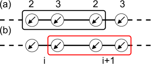
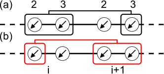
This expression means that all the $\sigma_{i,p}$ spins are coupled to an external magnetic field applied along direction $x+z$ and interact by a three-spin interaction depicted in Fig. 3, with signs given by the $r_{i}$ and $s_{i}$ quantum numbers. The structure of the interaction is such that we can consider the system as a set of interacting dimers labeled by $i$ consisting of spins $\sigma_{i,2}$ and $\sigma_{i,3}$. In the Appendix A we show the relation between $\sigma_{i,p}^{x,z}$ Pauli operators and the original ones, $X_{i,p}$ and $Z_{i,p}$, of Eq. (1).

Figure 3: (Color online) Schematic view of the interaction part of the Hamiltonian Eq. (14): (a) the $x$ interactions (black frame), and (b) the $z$ interactions (red frame). The arrows represent the ground state configuration of the spins $\sigma_{i,p}$ stabilized by the external field, under the assumption that the interaction part is absent.

Finally, it is worth to mention that the structure of the free and interaction terms in the Hamiltonian (14) is strongly related, i.e., we can find a basis where the linear terms become cubic and vice-versa. As there are twice as many linear terms as the cubic ones it is not possible to obtain a one-to-one correspondence between the free and interacting part of the Hamiltonian — in the Appendix B we give the additional interaction terms that should be added to obtain such duality as well as the form of the duality spin transformation.

III Perturbative treatment

The first question we may ask seeing the reduced Hamiltonian (14) of the 1D POM is in which subspace labeled by the $r_{i}$ and $s_{i}$ quantum numbers the ground state can be found. This can be easily answered by a perturbative expansion where the unperturbed Hamiltonian ${\cal H}_{0}$ is the noninteracting part of ${\cal H}$, i.e.,

$${\cal H}_{0}=\sum_{i=1}^{L}\left(\sigma_{i,2}^{z}+\sigma_{i,2}^{x}+\sigma_{i,3}^{z}+\sigma_{i,3}^{x}\right),$$ (15)

and the perturbation ${\cal V}$ is given by the three-spin terms,

$${\cal V}=\sum_{i=1}^{L}\!\left\{r_{i}\sigma_{i-1,3}^{z}\!\left(\sigma_{i,2}^{z}\sigma_{i,3}^{z}\right)\!+\!s_{i}\!\left(\sigma_{i,2}^{x}\sigma_{i,3}^{x}\right)\!\sigma_{i+1,2}^{x}\right\}.$$ (16)

The ground state of $\left|0\right\rangle$ of ${\cal H}_{0}$ is easy to infer, the spins order as in Fig. 3 with the ground state energy per dimer equal to

$$E_{0}^{(0)}=-2\sqrt{2}\simeq-0.282.$$ (17)

Hamiltonian ${\cal H}_{0}$ has a big energy gap of $\varepsilon_{1}=2\sqrt{2}$ which makes the expansion justified although formally there is no small parameter in ${\cal V}.$ The first order correction to the ground state energy is just the average of ${\cal V}$ in the state $\left|0\right\rangle$ which is simple to calculate as we deal with a simple product state. Thus we get a first order correction,

$$E_{0}^{(1)}=-\frac{1}{2\sqrt{2}L}\sum_{i=1}^{L}\left(r_{i}+s_{i}\right),$$ (18)

as a linear function of the quantum numbers $r_{i}$ and $s_{i}$. Now it is easy to see that the ground state of the model is in the subspace with $r_{i}=s_{i}=1$ for all $i$. This result also suggests that the lowest excited state of the model is the ground state from the subspace with one $r_{i}$ or $s_{i}$ flipped — such excitation costs the energy of $1/\sqrt{8}\approx 0.353$ in the leading order while the excitation within the lowest subspace costs the energy of $2\sqrt{2}\approx 2.828$ in the leading order.

As the first order correction cannot be regarded as small we now proceed to the higher orders. The second order correction has a form of,

$$E_{0}^{(2)}=-\frac{1}{L}\sum_{n\not=0}\frac{1}{\varepsilon_{n}}\left\langle 0\right|{\cal V}\left|n\right\rangle\left\langle n\right|{\cal V}\left|0\right\rangle,$$ (19)

where $\varepsilon_{n}=E_{n}^{(0)}-E_{0}^{(0)}$ is the excitation energy of the $n$-th excited state of ${\cal H}_{0}$. After a moderate analytical effort we can get a correction,

$$E_{0}^{(2)}=\frac{-1}{2^{4}3\sqrt{2}}\left\langle 6r_{i}r_{i+1}\!+\!6s_{i}s_{i+1}\!-\!9s_{i}r_{i+1}\!-\!9r_{i}s_{i}\!+\!29\right\rangle,$$ (20)

where the interaction terms between the classical spins are present and we take a contribution for the representative sites $i$ and $(i+1)$. The value of $E_{0}^{(2)}$ in the ground subspace is $E_{0}^{(2)}\approx-0.339$, the total ground state energy up to the second order is equal to

$$E_{0}^{(0)}+E_{0}^{(1)}+E_{0}^{(2)}\simeq-2.828-0.707-0.339=-3.874\,.$$ (21)

Such a value is problematic for, as we will see in the next Section, the extrapolated ground state energy from the exact diagonalization is equal to $E_{0}^{\rm ED}\simeq-3.7897$ which is higher than what we have obtained up to second order.

The above result and overall largeness of the second order correction indicates that we should go to the third order to get the energy within the physical range of values. The textbook expression for the third order energy correction reads,

$$E_{0}^{(3)}L \!=\! \sum_{n\not=m\not=0}\frac{1}{\varepsilon_{n}\varepsilon_{m}}\left\langle 0\right|{\cal V}\left|n\right\rangle\left\langle n\right|{\cal V}\left|m\right\rangle\left\langle m\right|{\cal V}\left|0\right\rangle$$ (22)

$$\!+\! \sum_{n\not=0}\frac{\left\langle n\right|{\cal V}\left|n\right\rangle-\left\langle 0\right|{\cal V}\left|0\right\rangle}{\varepsilon_{n}^{2}}\left\langle 0\right|{\cal V}\left|n\right\rangle\left\langle n\right|{\cal V}\left|0\right\rangle.$$

This already requires a considerable effort to calculate as due to the canted nature of the unperturbed ground state there are not many overlaps that cancel in the above expression. Probably the simplest way to calculate this correction is to span the Hilbert space of possible excited states for a given dimer $i$ in ${\cal V}$, define the operators in the product space and calculate the correction by a brute force. Here we used Mathematica to do it and the Hilbert space was a product space of $11$ with a dimension of $2^{11}$ and the $r_{i}$ and $s_{i}$ quantum numbers were kept as variables. The results is,

$$E_{0}^{(3)} \!=\! \frac{1}{2^{6}3\sqrt{2}}\left\langle 22\!\left(r_{i}\!+\!s_{i}\right)\!-\!3\!\left(r_{i}s_{i}r_{i+1}\!+\!s_{i}r_{i+1}s_{i+1}\right)\right\rangle$$ (23)

$$\!+\! \frac{1}{2^{13}3}\left\langle-29\left(r_{i}\!+\!s_{i}\right)\!-\!11\left(r_{i}s_{i}r_{i+1}\!+\!s_{i-1}r_{i}s_{i}\right)\right.$$

$$\!+\! 36\left.\left(r_{i-1}r_{i}s_{i}\!+\!s_{i-1}r_{i}r_{i+1}\!+\!s_{i-1}s_{i}r_{i+1}\!+\!r_{i}s_{i}s_{i+1}\right)\right.$$

$$\!-\! \left.24\left(r_{i-1}r_{i}r_{i+1}+s_{i-1}s_{i}s_{i+1}\right)\right\rangle,$$

where we take again an average contribution for the representative sites $i$ and $(i+1)$. Here the first line is a leading term that originates from the contributions where the two intermediate states are the same, i.e., $n=m$ — the second line of Eq. (22). The third order correction to the ground state is positive and equal to $E_{0}^{(3)}\approx 0.140$. Thus the ground state energy up to third order is $E_{0}^{\rm pert}\approx-3.734$ which is now well within the physical range given by the ED reported in Sec. V — the energy difference between this result and $E_{0}^{\rm ED}$ is of the order of $0.05$ so one can conclude that the third order expansion is almost exact.

Figure 4: (Color online) Ground state energies $E_{0}^{(p_{1},p_{2})}$ from the subspaces with two classical spins $p_{1,2}$ being excited; dots — $r_{10}$ and $r_{i}$ flipped, diamonds — $r_{10}$ and $s_{i}$ flipped and squares — $s_{10}$ and $r_{i}$ flipped, as functions of $i$. Dashed lines show the energies of single, double and triple energy gap $\Delta$.

Concerning the excitations, the energy gap given by the expansion is $\Delta^{\rm pert}=0.428$ which is close to the ED value of the gap $\Delta^{\rm ED}=0.437$, see below in Sec. V. As stated earlier, the first excited state is the ground state of the model in the subspace with one $r_{i}$ or $s_{i}$ being flipped. Eq. (18) and the value of $\Delta^{\rm pert}$ suggests that flipping two classical spins $r_{i}$ or $s_{i}$ should still cost less energy than creating an excitation within the ground subspace. We may expect that if the defects in the configuration of classical spins are sufficiently far from each other then the excitation energy should be $2\Delta^{\rm pert}$.

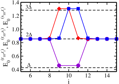
In Fig. 4 we show the excitation energies for one defect placed at site $i_{1}=10$ and second at any other site $i$ as a function of $i$. As at every site we have both $r_{i}$ and $s_{i}$ there are four possibilities of creating such a pair of defects because for each site we can flip $r_{i}$ or $s_{i}$. Due to the symmetry of Eq. (14) flipping two $r_{i}$’s is equivalent to flipping two $s_{i}$’s. As we can see from Fig. 4, all the excitation energies are close to $2\Delta$ when the defects are separated by more than two sites — this is additive regime governed by the first order correction of Eq. (18).

When the distance is smaller then we observe two different behaviors, the gap for $r$-$r$ (or $s$-$s$) excitation is smaller than expected and close to $\Delta$ and the gap for $s$-$r$ (or $r$-$s$) excitation is bigger than expected and close to $3\Delta$. In this regime the second and third order corrections are important. Such behavior means that flipping classical spins of different flavors at neighboring or the same sites is something that the system particulary dislikes. On the other hand, if we choose only one flavor to flip then Fig. 4 suggests that we could even flip all the $r_{i}$’s paying only one $\Delta$ of the excitation energy. The ED results show that this is not true (the higher order correction are important in this case) however they show that flipping all $r_{i}$’s still costs less energy than an excitation within the ground subspace.

Figure 5: (Color online) Local spin averages $\left\langle\sigma_{2,i}^{x,z}\right\rangle$ and $\left\langle\sigma_{3,i}^{x,z}\right\rangle$ shown as arrows in the: (a) global ground state, (b) first excited state with $r_{3}=-1$, and (c) first excited state with $s_{3}=-1$. The horizontal (vertical) components of the vectors (arrows) correspond to the $x$($z$) components of the spins $\sigma_{p,i}$. The frames indicate the dimers $\left\{\sigma_{2,i},\sigma_{3,i}\right\}$ with $i=1,2,3,4$.

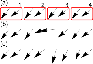
Finally, using the perturbation approach it is possible to look not only at the energies in different subspaces but also at the ground state spin configuration. It is quite simple to check that up to the first order the local spin averages are given by the following formulas,

$$\left\langle\sigma_{2,i}^{x}\right\rangle = -\frac{1}{\sqrt{2}}+\frac{2r_{i}-s_{i}-s_{i-1}}{4\sqrt{2}},$$

$$\left\langle\sigma_{2,i}^{z}\right\rangle = -\frac{1}{\sqrt{2}}+\frac{s_{i}-2r_{i}}{4\sqrt{2}},$$

$$\left\langle\sigma_{3,i}^{x}\right\rangle = -\frac{1}{\sqrt{2}}-\frac{s_{i}}{4\sqrt{2}},$$

$$\left\langle\sigma_{3,i}^{z}\right\rangle = -\frac{1}{\sqrt{2}}+\frac{s_{i}-r_{i+1}}{4\sqrt{2}}.$$ (24)

In Fig. 5 we show the above averages represented by the arrows for four sites $i=1,2,3,4$ with PBCs for the global ground state, shown in Fig. 5(a), and the lowest excited states with $r_{3}=-1$ and $s_{3}=-1$, see Figs. 5(b) and 5(c). In the ground state we observe a two-sublattice order where the configuration of neighboring spins differ by the interchange of the $x$ and $z$ component. In the excited states we observe distortion of the spin order being different for a flip in $r$ and $s$ spins. In the former case the $z$ components of the spins decrease when approaching the site with defect and then grow again. In the latter case the same happens to $x$ components so we can conclude that the two excitations are complementary (this is also visible in Fig. 4).

IV Mean-field treatment

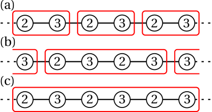
We have shown above that the excitation in the classical spins $r_{i}$ and $s_{i}$ are typically lower than a “quantum” excitation within the ground subspace. Such excited states are on the other hand the ground states of the reduced Hamiltonian (14) in the subspaces where some of the $r_{i}$’s or $s_{i}$’s are negative. This suggests that these states can be well described within a nonuniform MF approach carried out in any given subspace. The dimerized form of the Hamiltonian (14), see Fig. 3, suggests a MF approach where a main building block is a dimer. Thus if we think of a one-dimer approach we need to divide a system into clusters containing one dimer each (see Fig. 6(a)) or containing two, three dimers or more dimers [see Figs. 6(b) and 6(c)] if we think of a more general approach.

Clusterization means that the interactions within a cluster are treated exactly but different clusters interact only by MFs. This involves a standard decoupling of the interaction terms in the Hamiltonian (14) assuming that the correlations between the clusters are not strong, i.e.,

$$\left(\sigma_{i,2}^{x}\sigma_{i,3}^{x}\right)\sigma_{i+1,2}^{x} \simeq \left\langle\sigma_{i,2}^{x}\sigma_{i,3}^{x}\right\rangle\sigma_{i+1,2}^{x}+\sigma_{i,2}^{x}\sigma_{i,3}^{x}\left\langle\sigma_{i+1,2}^{x}\right\rangle$$ (25)

$$- \left\langle\sigma_{i,2}^{x}\sigma_{i,3}^{x}\right\rangle\left\langle\sigma_{i+1,2}^{x}\right\rangle,$$

$$\sigma_{i-1,3}^{z}\left(\sigma_{i,2}^{z}\sigma_{i,3}^{z}\right) \simeq \sigma_{i-1,3}^{z}\left\langle\sigma_{i,2}^{z}\sigma_{i,3}^{z}\right\rangle+\left\langle\sigma_{i-1,3}^{z}\right\rangle\sigma_{i,2}^{z}\sigma_{i,3}^{z}$$ (26)

$$- \left\langle\sigma_{i-1,3}^{z}\right\rangle\left\langle\sigma_{i,2}^{z}\sigma_{i,3}^{z}\right\rangle.$$

From this decoupling we have four independent MFs per dimer, i.e., $\left\langle\sigma_{i,2}^{x}\sigma_{i,3}^{x}\right\rangle$, $\left\langle\sigma_{i,2}^{z}\sigma_{i,3}^{z}\right\rangle$, $\left\langle\sigma_{i,2}^{x}\right\rangle$, and $\left\langle\sigma_{i,3}^{z}\right\rangle$. In the case when the configuration of the classical spins is uniform and the Hamiltonian (14) is translationally invariant we can safely assume that the above MFs do not depend on $i$ and the self-consistency equations can be solved for any system size $L$. This however is not the case in the excited subspaces that we are interested in. Thus, typically, we need to work with a finite system — here we have taken $L=100$.

Figure 6: (Color online) Schematic view of the dimer MF decoupling in case of: (a) one-dimer MF, (b) two-dimer MF and (c) three-dimer MF approximation. The frames mark the cluster of dimers that are treated exactly.

The self-consistency equations can be solved iteratively in each case, i.e., we set some random initial values of the MFs, then we diagonalize all the clusters and calculate new values of the MFs. The procedure is repeated until the desired convergence of the MFs is reached. In the majority cases this happens very quickly — after less than 100 iterations the old and the new value of each MF field does not differ by more than $10^{-14}$. This however does not refer to the subspaces with large areas being fully defected, i.e., for many neighboring sites $i$ we have $r_{i}=s_{i}=-1$. For instance, if we set all classical spins as $-1$ then the two interesting things happen within the MF approach: (i) within the uniform approach no convergence is reached and (ii) within a non-uniform approach we get a disordered configuration which depends on the initial values of the MFs. As we will see in the next Section such configuration is cured by the quantum fluctuations and the true ground state has a two-sublattice long-range order but with ordered moments that are strongly reduced with respect to the ground state configuration and, as it will be shown in Sec. V, strongly enhanced entanglement between the neighboring dimers. Finally, in order to check if the MF approximation is justified we can extend it in a perturbative manner. What is omitted in the MF approach are the correlation, so the full Hamiltonian ${\cal H}$ can be recovered from the MF one, ${\cal H}_{\rm MF}$, by adding the missing many-body term of the form,

$${\cal V}_{\rm corr} \!=\! \sum_{i=1}^{L}\left\{s_{i}\left(\sigma_{i,2}^{x}\sigma_{i,3}^{x}\!-\!\left\langle\sigma_{i,2}^{x}\sigma_{i,3}^{x}\right\rangle\right)\left(\sigma_{i+1,2}^{x}\!-\!\left\langle\sigma_{i+1,2}^{x}\right\rangle\right)\right.$$ (27)

$$\!+\! \left.r_{i}\left(\sigma_{i,2}^{z}\sigma_{i,3}^{z}\!-\!\left\langle\sigma_{i,2}^{z}\sigma_{i,3}^{z}\right\rangle\right)\left(\sigma_{i-1,3}^{z}\!-\!\left\langle\sigma_{i-1,3}^{z}\right\rangle\right)\right\}.$$

Now we can write that

$${\cal H}={\cal H}_{\rm MF}+{\cal V}_{\rm corr},$$ (28)

and treat the many-body term as a perturbation. Due to the self-consistency equations the first order correction to the energy vanishes. The calculation of the second order correction is elementary and requires the values of the MFs obtained earlier. It is significant that the value of this second order correction is less than $2\%$ of the MF energy in case of the ground state whereas it is almost $10\%$ of the MF energy for the fully defected subspace. This means that the simple MF approach works extremely well when no frustration is present and much worse when its magnitude is maximal.

Table 1: Summary of the ground state energies $E_{0}$ (per dimer) and the gap $\Delta$ obtained in the perturbation theory (up to third order) and within the MF approaches compared with the exact diagonalization results.

	approach	$E_{0}$	$\Delta$
	perturbation theory	$-3.734$	$0.428$
	1-dimer MF	$-3.6501$	$0.4134$
	2-dimer MF	$-3.7192$	$0.4520$
	3-dimer MF	$-3.7428$	$0.4592$
	1-dimer MF+correction	$-3.7022$	$\dots$
	exact diagonalization	$-3.789718$	$0.437271$

To summarize these energetic considerations we present the ground state energies obtained in perturbation theory and within the MF approach using a 1-dimer (with and without a second order correction), 2-dimer, and 3-dimer ansatz, respectively, compared to the value obtained by the exact diagonalization in Table I. This latter energy we believe to be the accurate one up to 6-digit precision (see Sec. V). As we can see, including one more dimer to the single-dimer MF improves the energy by roughly $0.06$ whereas the second correction gives $0.05$. On the other hand, adding another dimer lowers the energy to the value which is very close to the estimated value, the difference is of the order of $1\%$ only.

The excitation gap $\Delta$ requires good accuracy for both the ground state energy and the ground state in the subspace of the first excitation. Here the perturbation theory works somewhat better than the MF ansätze, see Table 1. The method we developed for the 1-dimer MF with a correction term (27) is reliable when the calculated state is unform, so it is not used to estimate the value of $\Delta$.

Figure 7: (Color online) Local spin averages $\left\langle\sigma_{2,i}^{x,z}\right\rangle$ and $\left\langle\sigma_{3,i}^{x,z}\right\rangle$ shown as arrows in different excited states with such classical spins flipped as indicated on the left. The horizontal (vertical) components of the vectors (arrows) correspond to the $x$($z$) components of the spins $\sigma_{p,i}$. The dimers $i=1,2$ are marked with different colors. The classical spins that are flipped are denoted on the left and the three last configurations with high excitation energies are marked with bold face.

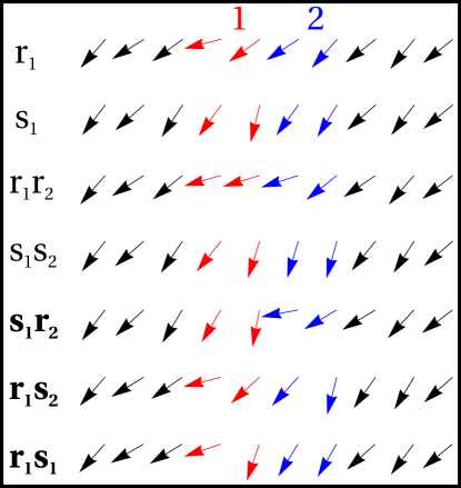
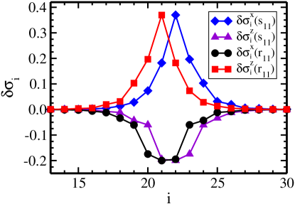
The MF spin configurations in the lowest excited states are shown in Fig. 7. First two lines show the effect of a single defect in $r_{i}$ and $s_{i}$ spins, respectively. These configurations are qualitatively similar to the perturbative ones shown in Fig. 5 but the range of the distortion caused by the defect is longer than before. In Fig. 8 we show the differences between these configurations and the ground state one — the distortion dies off at the distance of roughly $6$ spins ($3$ dimers). As shown in the plot of Fig. 4 the configurations with two defects have a doubled excitation energy with respect to the ones with single defect when the defects are far apart. In the next two lines of Fig. 7 we show the configurations with two defect only in $r_{i}$’s and only in $s_{i}$’s being next to each other. As we know from Fig. 4 such defects give a sub-additive energy close to a single energy gap. Fig 7 shows that these configurations are indeed very similar to the ones with single defects — the range of distortion is longer but the distortion itself is smoother. Finally, in the last three lines of Fig. 7 we show the two-defect cases when the excitation is increased above the additive level. These configurations are characterized by a rather severe spin distortion at the defects dimers which is related with the local frustration caused by the defects and is consistent with the increase of excitation energy.

According to Eq. (34) it is possible to uniquely relate the direction of the arrows shown in Fig. 7 with the values of bond operators of original ladder Hamiltonian of Eq. (1). $\sigma_{i,2}^{x}$ and $\sigma_{i,2}^{z}$ operators are the horizontal bonds within the $x$ and $z$ plaquettes respectively. Similarly, $\sigma_{i,3}^{x}$ and $\sigma_{i,3}^{z}$ are the vertical bonds within the $x$ and $z$ plaquettes. When an arrow points in the direction $-\left(x+z\right)$, as it happens in the ground state, it means that both $x$ and $z$ are locally satisfied. An arrow being more horizontal than the others indicates that locally the $x$ bonds are favored on expense of the $z$ ones. Analogically, a vertical tilt means that the $z$ bonds are favored.

Figure 8: (Color online) Differences in local spin averages in the excited states with $r_{11}=-1$ or $s_{11}=-1$ with respect to their ground state values, $\delta\sigma_{i}^{x,z}(r_{11})$ and $\delta\sigma_{i}^{x,z}(s_{11})$. Here we label the spins $\sigma_{2,i}$ and $\sigma_{3,i}$ by a single index $i$ so that $r_{11}$ and $s_{11}$ refer to $11$th dimer or spins $\sigma_{21}$ and $\sigma_{22}$.

As we can see from Fig. 7 excitation in $r_{i}$, which is related with the $z$ interaction term in the reduced Hamiltonian Eq. (14), transfers the energy from $z$ to $x$ bonds around site $i$. Excitation in $s_{i}$ has an inverse results. This we can understand very easily. Assume that in Eq. (14) we have only the part with $z$ Pauli operators. When all $r_{i}$ are positive than it is easy to check that in the ground state all spins will be pointing down and every term in the Hamiltonian will give a contribution $-1$ to the ground state energy. However if for one site $i$ we set $r_{i}=-1$ then the frustration occurs because the linear part of the Hamiltonian still wants all spins to point down whereas the cubic part for site $i$ has now an opposite sign and for such spin configuration gives a positive contribution to the energy. Thus the cubic term is frustrated with the linear terms. When the defect is only in the $r_{i}$ configuration then this frustration can be avoided by adjusting the spin configuration more to the $x$ part of the Hamiltonian and this exactly gives the horizontal tilt that we can see in the first line of Fig. 7. On the other hand when both $r_{i}$ and $s_{i}$ are locally negative then the frustration cannot be avoided and a severe distortion in the spin configuration occurs as shown in Fig. 7. In Sec. V we will demonstrate that such frustration can also lead to local disorder with increased quantum entanglement.

V Exact diagonalization treatment

Exact diagonalization was carried out using Lanczos algorithm for the system sizes up to $L=12$ for even $L$ and PBCs. In Fig. 9(a) we show finite size scaling of the ground state energies per dimer as function of $1/L$. Quite remarkably the energy saturates very quickly so the last four values are the same up to seven digits. A similar behavior is observed for the energy gap $\Delta$, see Fig. 9(b). Thus we can conclude that the values of the ground state energy (per dimer) and the energy gap obtained for $L=12$ are good approximations for the infinite system, these are:

$$E_{0}^{\rm ED} = -3.789718,$$ (29)

$$\Delta^{\rm ED} = 0.437271.$$ (30)

Figure 9: (Color online) Finite size scaling obtain for the POM: (a) ground state energy per dimer $E_{0}$, (b) energy gap $\Delta$, and (c) energy gap in the ground subspace $\Delta_{\rm GS}$.

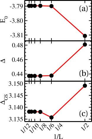
Although a gap within a ground-subpace $\Delta_{\rm GS}$, shown in Fig. 9(c), exhibits less regular scaling behavior but again a quick saturation is observed for the last three points so we can treat the last point as the thermodynamic limit, thus we have found that

$$\Delta_{\rm GS}^{\rm ED}=3.13816.$$ (31)

These values of the gaps confirm the perturbative results of Sec. III saying that the lowest energy excitations are the ones of the classical spins $r_{i}$, $s_{i}$ and the excitation within the ground subspace of the higher order of magnitude.

Probably the most interesting feature of the POM that cannot be captured within MF approaches is the spin configuration and entanglement in the highly defected subspaces, i.e., the subspaces where in certain range of $i$ both $r_{i}$ and $s_{i}$ are negative. In the extreme case of all $r_{i}$ and $s_{i}$ being negative it is not even possible to obtain conclusive MF results. In the ED approach we are free of such problems so in Fig. 10 we show the ground state spin configuration for $L=10$ dimers in the subspaces with a growing region of defects. The configurations are presented as the lines of arrows such that the first line corresponds with a ground subspace (no defects) and the last one with a fully defected subspace ($r_{i}=s_{i}=-1$ for all $i$). As we can see, the spins within the defected region (the red ones) seem to be disordered and change very rapidly from site to site. Some of them have even positive $x$ or $z$ components indicating the bonds that give positive contribution to the total energy (see discussion in Sec. IV), which implies strong frustration.

Figure 10: (Color online) Local spin averages $\left\langle\sigma_{2,i}^{x,z}\right\rangle$ and $\left\langle\sigma_{3,i}^{x,z}\right\rangle$ shown as arrows in subspaces with highly entangled areas where both $r_{i}$’s and $s_{i}$’s are negative (marked in red) for the system of the size $L=10$ obtained via ED; spin disorder increases from top to bottom. Every line corresponds with a different subspace, the first one with the ground subspace and the last one with the highest excited one. The horizontal (vertical) components of the vectors (arrows) correspond to the $x$($z$) components of the spins $\sigma_{p,i}$.

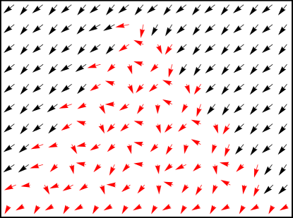
Interestingly, for defected region sizes $l$ that do not exceed $6$ dimers we observe a kind of regularity, a motif of four neighboring spins that repeats in an approximate fashion when the number of dimers in the defected region is even. This feature does not occur for larger regions except for the fully defected subspaces where the translational symmetry is present. In this case spins order regularly but the ordered moments are much smaller and the difference between sublattices is more pronounced than in the ground state configuration. Here the average values for the $p=2$ spins are $\langle\sigma_{2,i}^{x}\rangle\simeq-0.2985$ and $\langle\sigma_{2,i}^{z}\rangle\simeq-0.5419$ that give the ordered moment, $m=\{\langle\sigma_{2,i}^{x}\rangle^{2}+\langle\sigma_{2,i}^{z}\rangle^{2}\}^{1/2}=0.6187$. In the ground state these quantities are $\langle\sigma_{2,i}^{x}\rangle_{0}\simeq-0.7256$, $\langle\sigma_{2,i}^{z}\rangle_{0}\simeq-0.5846$, and $m_{0}=0.9318$. In both cases the configurations exhibit a two-sublattice translational invariant structure with the sublattices related by the interchange of the $x$ and $z$ components of spins. Similarly to the 2D Kugel-Khomskii model in the regime between the antiferromagnetic and ferromagnetic phase Brz12 , the spins seem to prefer being perpendicular to their neighbors but here because of the lower dimension this picture is more distorted by quantum fluctuations. Quite remarkably this classical view of perpendicular spins is realized by the quantum observables, i.e., we observe that in the fully defected subspace all the NN $\langle\sigma_{i}^{z}\sigma_{j}^{z}\rangle$ correlations and all the NN $\langle\sigma_{i}^{x}\sigma_{j}^{x}\rangle$ ones are equal to zero. This supports the picture of classical spin configuration where spins on one sublattice point along the $z$ axis and on the other one — along the $x$ axis. However the smallness of the ordered moments and the non-trivial angle between the spins in the configuration given by the ED indicate that this state is more complex and potentially highly entangled.

Figure 11: (Color online) Mutual information of the NN sites $I_{i,i+1}$ for different sizes $l$ of the highly defected area (shown in Fig. 10) as obtained for the chain of length $L=10$: (a) $l=1$ (dots), $l=2$ (diamonds) and $l=3$ (squares), (b) $l=4$ (dots), $l=5$ (diamonds), (c) $l=6$ (dots), $l=7$ (diamonds), and (d) $l=8$ (dots), $l=9$ (diamonds). The dashed lines are the values of $I_{i,i+1}$ in the ground subspace (bottom line) and in the totally defected subspace (upper line).

To quantify the entanglement of the states described in Fig. 10 we will look at the mutual information $I_{i,i+1}$ of the neighboring dimers in each of these states as function of the site index $i$. This quantity is defined by the von Neumann entropies of the dimers $i$, $i+1$ and pair of dimers $\left\{i,i+1\right\}$ as follows,

$$I_{i,i+1}={\cal S}_{i}+{\cal S}_{i+1}-{\cal S}_{i,i+1}$$ (32)

where the von Neumann entropy ${\cal S}_{A}$ of any subsystem $A$ is given by the formula,

$${\cal S}_{A}=-\mbox{Tr}\rho_{A}\log_{2}\rho_{A},$$ (33)

with $\rho_{A}$ being the reduced density matrix of the subsystem $A$ (i.e., we take the density matrix $\rho$ of the whole system and trace it over all degrees of freedom outside the subsystem $A$).

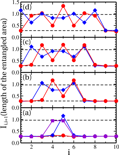
In Fig. 11 we present the mutual information $I_{i,i+1}$ for the states shown in Fig. 10 as function of $i$. The mutual information for the lowest and highest subspaces does not depend on $i$ and is equal to $I_{\rm GS}=0.28464$ and $I_{\rm HS}=0.96975$, respectively. These values prove that the ground state in the fully defected subspace is much more complex than the global ground state, as in the former the entanglement between the neighboring dimers is roughly three times stronger.

In the intermediate states that lie between the above two extremes the mutual information in the defected areas is always bigger than outside of them. This feature is very persistent in the sense that even if the area free of defects contains only one dimer then the mutual information of this dimer with respect to its neighbors is still roughly the same as in the ground state, see Fig. 11(d) — this refers of course also to other sizes of the defected area, compare Figs. 11(a), 11(b), 11(c) and 11(d). On the other hand, the mutual information inside the defected areas behaves less regularly; we may say that it has oscillatory character for the even sizes of the defected areas and more plateau-like character for odd sizes. This however is only a qualitative statement and probably larger systems should be studied to determine some universal features of $I_{i,i+1}$ inside the defected areas. What we can say for sure is that despite the observed oscillations, $I_{i,i+1}$ never drops below the ground state level $I_{\rm GS}$ in the defected areas although the value for the fully defected subspace $I_{\rm HS}$ can locally exceed it.

VI Summary and conclusions

We have shown a rather complete picture of the ground state and low-energy excitations of the one-dimensional plaquette orbital model defined by the Hamiltonian (1) using the perturbative, mean-field and exact diagonalization approaches. First the model was put in the block-diagonal form using spin transformation that reduces the size of the Hilbert space by a factor of two. In this way we have arrived at the model of interacting dimers consisting of the external field terms acting on every site and the interaction terms having the three-spin form, with signs given by the values of classical spins resulting from the spin transformations or the eigenvalues of the local symmetry operators. The perturbative approach has shown that the lowest energy is obtained by setting all classical spins up and the lowest excitations are obtained by creating defects in this polarized configuration of classical spins.

The ground state configuration of the effective quantum spins is characterized by the long-range order induced by the external field acting along $-(x+z)$ direction. We have shown that the local average values of these effective spins correspond with the average values of the bonds in the initial ladder so the long-range spin-spin correlations in the ground-subspace are the long-range bond-bond correlations in the $Cx$-$Cz$ model. This resembles the Néel order of the plaquettes energies found in the two-dimensional plaquette orbital model Wen09 , however it has been shown that this is an artifact of a deeper lying orientational order Bis10 . The polarized ground state configuration of the effective spins is slightly distorted by the quantum interaction terms that cause a two-sublattice modulation of the order such that the sublattices are related by the interchange of the $x$ and $z$ spin components.

In the lowest excited states the defects in the classical spins cause an additional distortion in the configuration of quantum spins through the local change of sign of the interaction terms. Such change produces always local frustration of the interaction term that in case of a single defect can be easily avoided by a local tilt of the spins along either $x$ or $z$ axis. However, in case of the two defects this is not always possible and the frustration can result in the super-additive increase in the excitation energy.

The inhomogeneous mean-field approach shows that the frozen distortions of the spin configuration found in the lowest excited states are very local; due to the external field terms the system returns to its ground state ordering at the distance of $3$ dimers. This is consistent with the exact diagonalization results indicating that quantum fluctuations have a short range character in the present model, as both the ground state energy per dimer and the gap saturate extremely fast with the increasing system size — already for $L=12$ both quantities provide excellent estimates for the values in the thermodynamic limit. This follows from finite spatial range of three-spin entanglement in the effective chain spin model makes also the mean field approaches very successful, as shown in Table 1. The energy gap remains finite for growing system size with the best estimate being $\Delta=0.437271$ Eq. (29), as obtained for $L=12$, and unlike in the 2D plaquette model Wen09 the ground state is unique. The ground state energy per dimer (or per one plaquette of the original model) is for this system $E_{0}=-3.789718$, see Eq. (30).

The strong locality of the model can be attributed to the fact that most of the bond operators of initial Hamiltonian are transformed into the external field terms. For this reason we can conclude about the behavior of the model from relatively small system sizes, in certain analogy to the critical quantum chains with Potts interactions Alc13 . This also makes the excitation within a ground subspace very costly as in the zeroth order we need to flip a spin against the external field to make an excitation. The estimation for such energy obtained by exact diagonalization, $\Delta_{\rm GS}=3.13816$, see Eq. (31), shows that it does not change much in the higher orders, at least not in the ground-subspace.

This not very exciting picture of mostly classical spin model found in the ground state changes drastically when the defects in classical spin configuration create frustration that cannot be avoided. This happens when for a given dimer $i$ both variables $r_{i}$ and $s_{i}$ are negative or both the $P_{i}^{z}$ and $P_{i}^{x}$ symmetries have negative eigenvalues. As we have seen from the mean-field approach and the exact diagonalization such a double defect produces a more severe distortion in the configuration of quantum spins and costs more energy (as also shown by the first order perturbation expansion) than these two defects separated by more than one dimer. Thus we have studied the spin configuration and the entanglement, characterized by the mutual information $I_{i,i+1}$ of the neighboring dimers, for the subspaces with such defects accumulated in the central part of the chain for a growing number of defected dimers. We have found that within the defected areas: (i) spins form a very irregular pattern that resembles a spin-glass state, and (ii) the mutual information $I_{i,i+1}$ is strongly increased with respect to its values outside the area. We note that this phenomenon is analogous to increasing entanglement entropy when disorder increases in quantum critical chains San06 .

There are two subspaces that are exceptional — the ground subspace where $I_{i,i+1}$ is (on average) minimal and equal to $I_{\rm GS}=0.28464$, and the fully excited subspace with $r_{i}=s_{i}=-1$ where $I_{i,i+1}$ is (on average) maximal and equal to $I_{\rm HS}=0.96975$. In both of these subspaces the ground states exhibit a two-sublattice long-range order, however in the latter the ordered moments are much smaller than in the former and the neighboring spins tend to be perpendicular to each other, i.e., the bond spin correlations vanish. The behavior of the mutual information $I_{i,i+1}$ in the intermediate subspaces is quite remarkable; no matter how large the defected area is, the mutual information for the dimers outside this area is always small and very close to $I_{\rm GS}$ - this also applies to the case when only one dimer is outside. On the other hand, on crossing the border of the defected area $I_{i,i+1}$ jumps immediately above $I_{\rm HS}$ and behaves in an oscillatory way within the area, remaining larger than $I_{\rm GS}$.

To conclude, we have constructed a simple pseudospin model where it is possible to obtain large areas of disorder (or a spin-glass-like behavior) and entanglement embedded in rather classically ordered surrounding only by tuning the values of the symmetry operators. We believe that this is of interest for constructing future quantum computing devices and the model could be realized by the superconducting lattices of Josephson junctions.

Appendix A Backward spin transformation

Having explicit form of the spin transformations given by Eqs. (4), (5), (10), (11) and (13), it is straightforward to find a direct tranformation from the new degrees of freedom, $\left\{\sigma_{i,2}^{z},\sigma_{i,3}^{z},r_{i},s_{i}\right\}$, to the old ones, $\left\{Z_{i,1},Z_{i,2},Z_{i,3},Z_{i,4}\right\}$, i.e.,

$$\sigma_{i,3}^{x} = X_{i,3}X_{i,4},$$

$$\sigma_{i,2}^{x} = X_{i,2}X_{i,3},$$

$$\sigma_{i,3}^{z} = Z_{i,1}Z_{i,4},$$

$$\sigma_{i,2}^{z} = Z_{i-1,1}Z_{i,2}.$$ (34)

The list is completed by the already known relations,

$$r_{i} = Z_{i,1}Z_{i,2}Z_{i,3}Z_{i,4},$$

$$s_{i} = X_{i+1,2}X_{i,1}X_{i,4}X_{i+1,3}.$$ (35)

Appendix B Duality of the interaction
and the free term

It is easy to notice that the form of the spin interaction in Eq. (14) that the three-spin terms behave as new Pauli operators, in the sense that they satisfy all the canonical commutation relations. Thus we can define new spins, $\tau_{i,p}$ as follows,

$$\tau_{i,2}^{x} = s_{i-1}\left(\sigma_{i-1,2}^{x}\sigma_{i-1,3}^{x}\right)\sigma_{i,2}^{x},$$

$$\tau_{i,3}^{z} = r_{i+1}\sigma_{i,3}^{z}\left(\sigma_{i+1,2}^{z}\sigma_{i+1,3}^{z}\right).$$ (36)

Here we just took the interaction terms from Eq. (14) or at those shown in Fig. 3. However, the algebra is not complete yet, we need to define the $z$ and $x$ counterparts of the $\tau_{i,2}^{x}$ and $\tau_{i,3}^{z}$ operators. One can easily check that these definitions should be,

$$\tau_{i,2}^{z} = r_{i+1}\sigma_{i,2}^{z}\left(\sigma_{i+1,2}^{z}\sigma_{i+1,3}^{z}\right),$$

$$\tau_{i,3}^{x} = s_{i-1}\left(\sigma_{i-1,2}^{x}\sigma_{i-1,3}^{x}\right)\sigma_{i,3}^{x}.$$ (37)

Having them one can transform ${\cal H}$ to find

$${\cal H} = \sum_{i=1}^{L}\left\{\,\tau_{i,2}^{x}+\tau_{i,3}^{z}\right.$$ (38)

$$+ r_{i}\tau_{i-1,3}^{z}\left(\tau_{i,2}^{z}\tau_{i,3}^{z}\right)+s_{i}\left(\tau_{i,2}^{x}\tau_{i,3}^{x}\right)\tau_{i+1,2}^{x}$$

$$+ \left.r_{i}\tau_{i-1,2}^{z}\left(\tau_{i,2}^{z}\tau_{i,3}^{z}\right)+s_{i}\left(\tau_{i,2}^{x}\tau_{i,3}^{x}\right)\tau_{i+1,3}^{x}\,\right\}.$$

Figure 12: (Color online) Schematic view of the interactions in Eq. (39) complementary to the ones present in Eq. (14) — see Fig. 3: (a) the $x$ interactions (black frames), and (b) the $z$ interactions (red frames).

This Hamiltonian has a very similar structure to the one of Eq. (14), i.e., we have linear terms in $\tau_{i,p}$ and cubic interaction terms with signs given by $r_{i}$ and $s_{i}$. There is also a subtle difference as we get two more interaction terms [third line of Eq. (38)] compared to the one already present in Eq. (14) but lose two of the linear terms. It is straightforward to check that the structure of the two Hamiltonians is exactly the same if we add to the Hamiltonian Eq. (14) interaction terms of the complementary form, $r_{i}\sigma_{i-1,2}^{z}\left(\sigma_{i,2}^{z}\sigma_{i,3}^{z}\right)$ and $s_{i}\left(\sigma_{i,2}^{x}\sigma_{i,3}^{x}\right)\sigma_{i+1,3}^{x}$, see Fig. 12. In the other words, the Hamiltonian ${\cal H}_{\rm inv}$ of the form,

$${\cal H}_{\rm inv} = \sum_{i=1}^{L}\left\{\left(\sigma_{i,2}^{z}+\sigma_{i,3}^{z}\right)+\left(\sigma_{i,2}^{x}+\sigma_{i,3}^{x}\right)\right.$$ (39)

$$+ r_{i}\left(\sigma_{i-1,2}^{z}+\sigma_{i-1,3}^{z}\right)\left(\sigma_{i,2}^{z}\sigma_{i,3}^{z}\right)$$

$$+ \left.s_{i}\left(\sigma_{i,2}^{x}\sigma_{i,3}^{x}\right)\left(\sigma_{i+1,2}^{x}+\sigma_{i+1,3}^{x}\right)\right\},$$

is invariant under spin transformations (36) and (B).

References

- (1) Y. Tokura and N. Nagaosa, Science 288, 462 (2000).
- (2) J. van den Brink, Z. Nussinov, and A. M. Oleś, in: Introduction to Frustrated Magnetism: Materials, Experiments, Theory, edited by C. Lacroix, P. Mendels, and F. Mila (Springer, New York, 2011).
- (3) A. M. Oleś, G. Khaliullin, P. Horsch, and L. F. Feiner, Phys. Rev. B 72, 214431 (2005).
- (4) G. Khaliullin, Prog. Theor. Phys. Suppl. 160, 155 (2005).
- (5) A. M. Oleś, J. Phys.: Condens. Matter 24, 313201 (2012).
- (6) K. I. Kugel and D. I. Khomskii, JETP 37, 725 (1973); Sov. Phys. Usp. 25, 231 (1982).
- (7) L. Amico, R. Fazio, A. Osterloh, and V. Vedral, Rev. Mod. Phys. 80, 517 (2008).
- (8) A. M. Oleś, P. Horsch, L. F. Feiner, and G. Khaliullin, Phys. Rev. Lett. 96, 147205 (2006); W.-L. You, A. M. Oleś, and P. Horsch, Phys. Rev. B 86, 094412 (2012).
- (9) P. Horsch, A. M. Oleś, L. F. Feiner, and G. Khaliullin, Phys. Rev. Lett. 100, 167205 (2008).
- (10) J. Sirker, A. Herzog, A. M. Oleś, and P. Horsch, Phys. Rev. Lett. 101, 157204 (2008); A. Herzog, P. Horsch, A. M. Oleś, and J. Sirker, Phys. Rev. B 83, 245130 (2011).
- (11) B. Normand and A. M. Oleś, Phys. Rev. B 78, 094427 (2008); J. Chaloupka and A. M. Oleś, ibid. 83, 094406 (2011).
- (12) W. Brzezicki, J. Dziarmaga, and A. M. Oleś, Phys. Rev. Lett. 109, 237201 (2012); Phys. Rev. B 87, 064407 (2013).
- (13) S. Di Matteo, G. Jackeli, C. Lacroix, and N. B. Perkins, Phys. Rev. Lett. 93, 077208 (2004); G.-W. Chern and C. D. Batista, ibid. 107, 186403 (2011).
- (14) Y. Q. Li, M. Ma, D. N. Shi, and F. C. Zhang, Phys. Rev. Lett. 81, 3527 (1998); B. Frischmuth, F. Mila, and M. Troyer, ibid. 82, 835 (1999).
- (15) W. Brzezicki, J. Dziarmaga, and A. M. Oleś, Phys. Rev. Lett. 112, 117204 (2014).
- (16) J. van den Brink, P. Horsch, F. Mack, and A. M. Oleś, Phys. Rev. B 59, 6795 (1999).
- (17) J. van den Brink, New J. Phys. 6, 201 (2004).
- (18) L. F. Feiner and A. M. Oleś, Phys. Rev. B 71, 144422 (2005).
- (19) A. van Rynbach, S. Todo, and S. Trebst, Phys. Rev. Lett. 105, 146402 (2010).
- (20) M. Daghofer, K. Wohlfeld, A. M. Oleś, E. Arrigoni, P. Horsch, Phys. Rev. Lett. 100, 066403 (2008); K. Wohlfeld, M. Daghofer, A. M. Oleś, P. Horsch, Phys. Rev. B 78, 214423 (2008).
- (21) P. Wróbel and A. M. Oleś, Phys. Rev. Lett. 104, 206401 (2010); P. Wróbel, R. Eder, and A. M. Oleś, Phys. Rev. B 86, 064415 (2012).
- (22) F. Trousselet, A. Ralko, and A. M. Oleś, Phys. Rev. B 86, 014432 (2012).
- (23) G. Chen and L. Balents, Phys. Rev. Lett. 110, 206401 (2013).
- (24) Z. Nussinov and J. van den Brink, arXiv:1303.5922 (unpublished).
- (25) Z. Nussinov and E. Fradkin, Phys. Rev. B 71, 195120 (2005).
- (26) B. Douçot, M. V. Feigel’man, L. B. Ioffe, and A. S. Ioselevich, Phys. Rev. B 71, 024505 (2005).
- (27) J. Dorier, F. Becca, and F. Mila, Phys. Rev. B 72, 024448 (2005).
- (28) T. Tanaka and S. Ishihara, Phys. Rev. Lett. 98, 256402 (2007).
- (29) S. Wenzel and W. Janke, Phys. Rev. B 78, 064402 (2008).
- (30) R. Orús, A. C. Doherty, and G. Vidal, Phys. Rev. Lett. 102, 077203 (2009).
- (31) J. Vidal, R. Thomale, K. P. Schmidt, and S. Dusuel, Phys. Rev. B 80, 081104 (2009).
- (32) L. Cincio, J. Dziarmaga, and A. M. Oleś, Phys. Rev. B 82, 104416 (2010).
- (33) W. Brzezicki and A. M. Oleś, Phys. Rev. B 82, 060401 (2010); 87, 214421 (2013).
- (34) F. Trousselet, A. M. Oleś, and P. Horsch, Europhys. Lett. 91, 40005 (2010); Phys. Rev. B 86, 134412 (2012).
- (35) W. Brzezicki, J. Dziarmaga, and A. M. Oleś, Phys. Rev. B 75, 134415 (2007); W. Brzezicki and A. M. Oleś, Acta Phys. Polon. A 115, 162 (2009).
- (36) W.-L. You, P. Horsch, and A. M. Oleś, Phys. Rev. B 89, 104425 (2014).
- (37) W. Brzezicki and A. M. Oleś, Phys. Rev. B 80, 014405 (2009).
- (38) A. Kitaev, Annals of Physics 321, 2 (2006).
- (39) G. Baskaran, S. Mandal, and R. Shankar, Phys. Rev. Lett. 98, 247201 (2007).
- (40) S. Wenzel and W. Janke, Phys. Rev. B 80, 054403 (2009).
- (41) M. Biskup and R. Kotecký, J. Stat. Mech.: Theory and Experiment P11001 (2010).
- (42) F. C. Alcaraz and M. A. Rajabpour, Phys. Rev. Lett. 111, 017201 (2013).
- (43) Raoul Santachiara, J. Stat. Mech.: Theory and Experiment P06002 (2006).