Homogenization Model for Aberrant Crypt Foci

Abstract– Several explanations can be found in the literature about the origin of colorectal cancer. There is however some agreement on the fact that the carcinogenic process is a result of several genetic mutations of normal cells. The colon epithelium is characterized by millions of invaginations, very small cavities, called crypts, where most of the cellular activity occurs. It is consensual in the medical community, that a potential first manifestation of the carcinogenic process, observed in conventional colonoscopy images, is the appearance of Aberrant Crypt Foci (ACF). These are clusters of abnormal crypts, morphologically characterized by an atypical behavior of the cells that populate the crypts. In this work an homogenization model is proposed, for representing the cellular dynamics in the colon epithelium. The goal is to simulate and predict, in silico, the spread and evolution of ACF, as it can be observed in colonoscopy images. By assuming that the colon is an heterogeneous media, exhibiting a periodic distribution of crypts, we start this work by describing a periodic model, that represents the ACF cell-dynamics in a two-dimensional setting. Then, homogenization techniques are applied to this periodic model, to find a simpler model, whose solution symbolizes the averaged behavior of ACF at the tissue level. Some theoretical results concerning the existence of solution of the homogenized model are proven, applying a fixed point theorem. Numerical results showing the convergence of the periodic model to the homogenized model are presented.

Keywords - Homogenization, convection-diffusion equations, fixed-point theorem, cell dynamics, colon.

Mathematics Subject Classification (2010):
76R99, 35J15, 35B27, 47H10, 65M06, 65M50, 65M60

1 Introduction

Colorectal cancer is one of the most common types of malignant tumors in the Western World [62]. It is generally accepted that its origin is associated with an accumulation of genetic mutations at the cellular level that occur inside small cavities, called crypts, located in the colon epithelium.

Despite the high rate of cancer mortality after detection, it is possible to reduce the effects of this disease through an early diagnosis. This is due to the amount of time, 20 to 40 years according to [44], that elapses between the genetic mutations, that are at the origin of this process, and the outbreak of the carcinoma. During this process some adenomas (that are benign epithelial tumors) develop and if detected and removed cancer can be avoided.

There are different ways to address the morphogenesis of the colorectal cancer. Most of the approaches rely on experimental works (see e.g. [3]) that are then traduced in mathematical models. The reader can refer to [34, 39, 44, 65, 66, 68] for a review of colorectal cancer models. It is believed that the precursors of colorectal cancer are Aberrant Crypt Foci (ACF) [8, 9]. These latter are clusters of crypts in the colon epithelium, containing cells with a deviant behavior with respect to the normal ones. There is no agreement regarding the morphogenesis of ACF. Two major mechanisms have been proposed: top-down and bottom-up morphogenesis. In the first, see [42, 61], the abnormal cells are, at the beginning, in a superficial portion of the mucosae and after spread laterally and downwards inside the crypt. The bottom-up morphogenesis [42, 54] relies on the property that the bottom of the crypt is the most active region for cell division and genetic alterations and therefore assumes that the appearance of abnormal cells occurs in this region. In [54] a combination of these two mechanisms has been considered, wherein an abnormal cell located in the crypt base migrates to the crypt orifice, as in the bottom-up morphogenesis, and then it spreads laterally filling the adjacent crypts in agreement to the top-down morphogenesis. For a review of ACF medical analysis and colorectal cancer the reader can refer to [24, 30, 36, 54, 56, 61, 64].

We now briefly explain our main motivation for doing this work and the main goal. Conventional colonoscopy is a current medical technique used in gastroenterology to detect in vivo ACF. The colonoscopy images give a top view of the colon wall, at the tissue level, and from the endoscopic point of view, ACF stain darker than normal crypts when some dyes (as for instance, methylene blue) are instilled in the colon (during the colonoscopy exam). The medical Figure 1 shows a colonoscopy image exhibiting two ACF : the two large dark round objects, each comprising hundreds of aberrant crypts. In this figure we can also observe the small circles spread all over the image that represent the top crypt orifices (directed to the lumen of the colon), and we can clearly perceive a periodic distribution of crypts in the colon wall (the dot like orifices that are densely distributed).

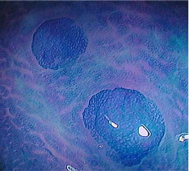
Figure 1: Colonoscopy image (obtained with a conventional endoscope), showing two large ACF in the human colon of a patient (Courtesy: Faculty of Medicine, University of Coimbra, Portugal).

The main motivation of this work is to model the evolution of ACF, i.e., the evolution of groups of several aberrant crypts, as observed in colonoscopy images. Our goal is to reproduce in silico the dynamics of ACF at the macroscopic tissue level, by using appropriate mathematical models and tools. To this end, we propose a cell dynamics model for describing the evolution of abnormal colonic cells in a single crypt, and subsequently, using the periodic structure of the colon, we resort to homogenization techniques for simulating the evolution of ACF at the tissue level in a two-dimensional framework. In particular, the cell dynamics model used is a PDE (partial differential equation) model that confines itself to two populations of colonic cells, normal and abnormal, and that is afterwards re-written only in terms of the abnormal cell population.

We give now a brief overview of the approach followed in this paper for modeling ACF dynamics. The colon is modeled as an heterogeneous two-dimensional medium perforated by crypts, that are periodically distributed. The heterogeneous periodic model, used in this work, to represent the ACF evolution in the colon is similar to that presented in [23], with the difference that in this work an hexagonal region representing each crypt is used (as done in [32]) instead of a square. The model is described in detail in Sections 2, 3 and 4.1. It consists of a system coupling a parabolic and an elliptic equation, whose unknowns are respectively, the density of abnormal cells and the pressure generated by cell proliferation. We assume that these abnormal cells have the property to proliferate not only inside the crypt as done by normal cells, but also outside. This property is believed to be responsible for abnormal cells to invade neighbor crypts and can induce crypt fission and the formation of an adenoma [25, 54, 66]. In this work crypt fission is not considered, due to limitations of the chosen homogenization technique, a two-scale asymptotic expansion method (see Section 4). Then, by using an heuristic procedure, we derive the corresponding homogenized model. It is again a system coupling a parabolic and an elliptic equation, whose unknown is the pair (abnormal cell density, pressure) corresponding to the first terms of the two-scale asymptotic expansions. Based on fixed-point type arguments, the existence of solution of the homogenization model is proved. We remark that, the complexity of the problem does not permit a proof of the convergence of the periodic model to the homogenized one, though this is verified by the numerical tests we have performed.

After this introduction, the layout of the paper is as follows. In Section 2 we define the three-dimensional (3D) crypt geometry as well as its reformulation as a two-dimensional domain (2D), using a suitable bijection operator. In Section 3 the crypt cell dynamics model is described as well as its reformulation in a 2D framework. In Section 4 we extend this crypt cell dynamics model by periodicity to obtain an heterogeneous and periodic model for the colon. The homogenization technique, based on the heuristic two-scale asymptotic expansion method (ansatz), is applied to this heterogeneous model to obtain the homogenization model. In Section 5, the existence of solution to the homogenization model is proved, as shown in Theorem 5.1. The approximate solution to the homogenized model, that uses finite elements for the space variable and finite differences for the time variable, is described in Section 6. The numerical simulations are presented in Section 7, and finally some conclusions and future work are outlined.

2 Crypt geometry (3D and 2D)

Each crypt has a test-tube shaped structure, closed at the bottom and open at the top. According to [32, 33], the average dimensions for a human colonic crypt are $433\,\mu m$ ($1\mu m=10^{-6}m$), from the bottom to the top, and $16\,\mu m$ for the diameter of the top orifice excluding the epithelium, with a cell depth of $15.1\mu m$. In this work, we approximate the geometry of a single crypt with a flat-bottomed cylinder $S\subset\mathbb{R}^{3}$, as done in other works (see e.g. [46]). The cylinder $S$ is composed of three main parts $S:=S_{1}\cup S_{2}\cup S_{3}$ (represented in Figure 2, left and defined in (1)). Note that we identify the crypt with the region $S$, where $S_{1}$ (a regular hexagonal region of edge $a$) is the inter-cryptal region around the crypt orifice, $S_{2}$ and $S_{3}$ represent, respectively, the lateral and the bottom region of the cylinder-like structure, with radius $R$ and height $L>0$ (for the numerical simulations, in Section 7, we assume a relation between the diameter $2R$ and the height $L$, in good agreement with the average dimensions of a single crypt).

$$\begin{array}[]{l}S_{1}:=\left\{(x_{1},x_{2},x_{3})\in\mathbb{R}^{3}:(x_{1},x_{2})\in{\rm regular\ hexagon\ of\ edge\ }a,\ \sqrt{x_{1}^{2}+x_{2}^{2}}>R,\ \mbox{and}\ x_{3}=L\right\}\\[7.5pt] S_{2}:=\left\{(x_{1},x_{2},x_{3})\in\mathbb{R}^{3}:\sqrt{x_{1}^{2}+x_{2}^{2}}=R\,\,\,\mbox{and}\,\,\,x_{3}\in]0,L]\right\}\\[7.5pt] S_{3}:=\left\{(x_{1},x_{2},x_{3})\in\mathbb{R}^{3}:\sqrt{x_{1}^{2}+x_{2}^{2}}\leq R\,\,\,\mbox{and}\,\,\,x_{3}=0\right\}.\end{array}$$ (1)

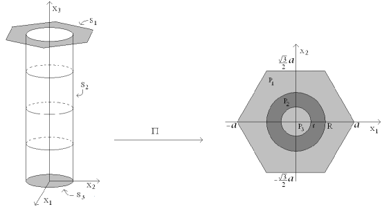
Figure 2: Left: Schematic representation of a region $S=S_{1}\cup S_{2}\cup S_{3}$ in the colon, containing a 3D crypt and a small surrounding neighborhood (depicted by $S_{1}$). Right: The hexagonal region $P$ obtained by the projection of $S$ in a plane with the operator $\Pi$, where $P_{i}:=\Pi(S_{i})$ for $i=1,2,3$.

For the subsequent work herein (in order to define a 2D model for the ACF evolution) it is necessary to reformulate the crypt geometry $S\subset\mathbb{R}^{3}$ as a plane domain $P$, that is defined as a regular hexagon, with area, $|P|$, equal to 1, and with edge $a=\frac{\sqrt{2}}{3^{\frac{3}{4}}}$, by using the following bijective projection operator $\Pi$ from $S$ to $P$, defined by

$$\Pi(x_{1},x_{2},x_{3}):=\begin{array}[]{lccl}\left\{\begin{array}[]{lcl}(x_{1},x_{2})&\rm if&(x_{1},x_{2},x_{3})\in S_{1}\\[7.5pt] \displaystyle\left(\frac{1}{R}\left[r+\frac{x_{3}}{L}(R-r)\right]x_{1},\frac{1}{R}\left[r+\frac{x_{3}}{L}(R-r)\right]x_{2}\right)&\rm if&(x_{1},x_{2},x_{3})\in S_{2}\\[9.49997pt] \displaystyle\frac{r}{R}(x_{1},x_{2})&\rm if&(x_{1},x_{2},x_{3})\in S_{3}.\end{array}\right.\end{array}$$ (2)

The projection $\Pi$ applies $S$ in $P:=P_{1}\cup P_{2}\cup P_{3}$, where $P_{i}=\Pi(S_{i})$. We remark that $\Pi$ shrinks the bottom $S_{3}$ of the crypt into a circle with radius $r$ (verifying $0<r<R$), defined by $P_{3}$, while the lateral part $S_{2}$ of the crypt is projected in the region $P_{2}$, that lies between the circles with radius $r$ and $R$.

For any arbitrary function $g$ defined in $S\subset\mathbb{R}^{3}$, the corresponding function $g^{*}$ defined in $\Pi(S)=P\subset\mathbb{R}^{2}$ is given by

$$g^{*}(X_{1},X_{2})=g(x_{1},x_{2},x_{3})\quad{\rm with}\quad(X_{1},X_{2})={\Pi}(x_{1},x_{2},x_{3}).$$ (3)

Moreover the following relations, between the old and new variables, hold

$$\begin{array}[]{lcl}\mbox{in}\quad S_{1}&&(x_{1},x_{2})=(X_{1},X_{2}),\\ \\ \mbox{in}\quad S_{2}&&\left\{\begin{array}[]{l}x_{1}=\displaystyle\frac{R\,X_{1}}{\sqrt{X_{1}^{2}+X_{2}^{2}}}\\ \\ x_{2}=\displaystyle\frac{R\,X_{2}}{\sqrt{X_{1}^{2}+X_{2}^{2}}}\\ \\ x_{3}=\displaystyle\frac{L}{R-r}\big{(}\sqrt{X_{1}^{2}+X_{2}^{2}}-r\big{)},\\ \end{array}\right.\\ \\ \mbox{in}\quad S_{3}&&(x_{1},x_{2})=\displaystyle\frac{R}{r}(X_{1},X_{2}).\end{array}$$ (4)

As a consequence, the following relations between the partial derivatives of $g$ and $g^{*}$ also hold

$$\begin{array}[]{lcl}\mbox{in}\quad S_{1}&&\displaystyle\big{(}\frac{\partial g}{\partial x_{1}},\frac{\partial g}{\partial x_{2}},\frac{\partial g}{\partial x_{3}}\big{)}=\displaystyle\big{(}\frac{\partial g^{*}}{\partial X_{1}},\frac{\partial g^{*}}{\partial X_{2}},0\big{)},\\ \\ \mbox{in}\quad S_{2}&&\left\{\begin{array}[]{l}\displaystyle\frac{\partial g}{\partial x_{1}}=\displaystyle\frac{1}{R}\left(r+\frac{x_{3}}{L}(R-r)\right)\frac{\partial g^{*}}{\partial X_{1}}\\ \\ \displaystyle\frac{\partial g}{\partial x_{2}}=\displaystyle\frac{1}{R}\left(r+\frac{x_{3}}{L}(R-r)\right)\frac{\partial g^{*}}{\partial X_{2}}\\ \\ \displaystyle\frac{\partial g}{\partial x_{3}}=\displaystyle\frac{R-r}{RL}\big{(}x_{1}\frac{\partial g^{*}}{\partial X_{1}}+x_{2}\frac{\partial g^{*}}{\partial X_{2}}\big{)},\\ \end{array}\right.\\ \\ \mbox{in}\quad S_{3}&&\displaystyle(\frac{\partial g}{\partial x_{1}},\frac{\partial g}{\partial x_{2}},\frac{\partial g}{\partial x_{3}})=\frac{r}{R}(\frac{\partial g^{*}}{\partial X_{1}},\frac{\partial g^{*}}{\partial X_{2}},0).\end{array}$$ (5)

3 Colonic crypt cell model (3D and 2D)

Each crypt is a compartment containing different types of cells. These are aligned along the crypt wall: stem cells are believed to reside in the bottom of the crypt, transit cells along the middle part of the crypt axis and differentiated cells at the top of the crypt. In normal human colonic crypts, the cells renew completely each 5-6 days [58], through an harmonious and ordered procedure which includes the proliferation of cells, their migration along the crypt wall towards the top and their apoptosis, as they reach the orifice of the crypt.

It is generally believed that a sequence of genetical mutations and alterations in the sub-cellular mechanisms can evolve later into colorectal cancer [7, 44, 65, 68]. In the literature there are many mathematical models proposed for reproducing the colonic cell dynamics. We refer, for example, to the interesting and useful reviews [11, 39, 65]. These models can be divided in two large groups: compartmental and spatial models.

The compartmental models track the populations of different types (compartments) of colorectal cells (usually stem, semi-differentiated and differentiated cells) by using systems of ordinary differential equations as in [10, 38] or by stochastic models [41, 43]. These compartmental approaches determine, in each time, the number of cells of each population, and allow cells to enter or leave the compartments without specifying the relative spatial location of cells in the crypt. These models cannot describe then the cell migration and the spatial influence of proliferation or death rate parameters, as opposed to spatial models that can incorporate these effects. The group of spatial models can be divided in two subgroups: cell-based models and continuum models. In cell-based models, the cell dynamics is given by a finite number of mechanical forces and protein concentrations among other quantities. Moreover, some probability of dividing or moving cells in certain directions can be used, as well as the passage of a mutation characteristic, therefore, as in [26, 37, 46, 53, 67], stochastic models coupled with deterministic relations are used. Since these models treat cells as distinct entities they are able to incorporate sub-cellular features as cell-cell and cell-membrane adhesions, signaling pathways and protein level models [39, 68]. The disadvantage of these approaches is that they are computationally expensive and need a lot of experimental parameters that are difficult to collect. Continuum models measure the cell populations by their densities and use few parameters and computations to describe the continuum dynamics of cells. Continuum models are usually defined by systems of partial differential equations to characterize the cell features and are very popular for modeling avascular tumor growth [2, 15, 14, 57, 60, 69] or tissue growth [40]. These models are used to simulate only the crypt cell dynamics [21, 47, 48, 50, 68] or the crypt dynamics (budding and fission) [16, 17, 22] based on a cell dynamics model.

A continuum model was proposed in [23] for describing the abnormal cell dynamics in the 3D crypt domain $S\subset\mathbb{R}^{3}$ and, through its reformulation in the 2D domain $P=\Pi(S)\subset\mathbb{R}^{2}$ (these two domains were introduced in Section 2). In this section we define a similar model, that will be used subsequently for deriving the homogenization model.

According to [44] “Two scenarios of cellular dynamics within a colonic crypt are possible. In the first scenario, only colorectal stem cells are considered to be at risk of becoming cancer cells [49]. In the second scenario, all cells of the colonic crypt are assumed to be at risk of accumulating mutations that lead to cancer [45]. Mutations in specific genes might confer an increased probability to the cell to stick on top of the crypt instead of undergoing apoptosis”. In this work, we assume this second scenario, since it is in good agreement with medical information obtained through the colonoscopy images and correspondent biopsies, performed during the colonoscopy exam [25].

In healthy (normal) colonic crypts the cells are distributed in the following way: i) in the bottom there are stem cells with a high proliferative rate, ii) in the middle there are semi-differentiated cells, that also proliferate but with a lower rate than stem cells, iii) at the top of the crypt there are fully differentiated cells, that do not reproduce themselves.

In our prototype model we start by considering that there exist two main classes of colonic cells, normal with density $N$ and abnormal with density $C$. A normal cell has a proliferative rate in good agreement with its location in the crypt (middle, bottom or top). An abnormal cell is a proliferative cell that does not have a normal proliferative rate. For instance, if at the top of the crypt there are cells that reproduce themselves, then these are abnormal cells. Furthermore we assume that the two types of cells verify the overall density hypothesis $N+C=1$ (and $0\leq N,C\leq 1$). This is equivalent to supposing that no free-space exists and that normal and abnormal cells have the same volume. This is often used in the context of living tissue growth [40, 51] and for modeling tumor growth [29, 55, 60, 69]. This hypothesis is appropriate for modeling early stages of development of abnormal cells, as it is our intention in this work, but in advanced stages a condition involving an increase of volume could also be envisaged.

Let us denote by $t$ the time variable belonging to the interval $[0,T]$, with $T>0$ fixed, and by $N(x_{1},x_{2},x_{3},t)$ and $C(x_{1},x_{2},x_{3},t)$, respectively, the normal and abnormal cell densities, at each point $(x_{1},x_{2},x_{3})$ of $S$ and at time $t$. Thus, for the overall density hypothesis , $N(x_{1},x_{2},x_{3},t)$ and $C(x_{1},x_{2},x_{3},t)$ represent the percentage of normal and abnormal cells at the spatial point $(x_{1},x_{2},x_{3})$ and time $t$. Then, based on models of tumor growth, described by systems of PDEs and relying on transport/diffusion/reaction models (see for instance [40], also [29, 50, 57] and [4, 13]), we propose the following system of PDEs for representing the dynamics of these populations of colonic cells in $S\times(0,T)$

$$\left\{\begin{array}[]{lcl}\displaystyle\frac{\partial N}{\partial t}+\nabla\cdot(v_{N}\,N)&=&\nabla\cdot(D_{N}\nabla N)+\gamma N,\\[7.5pt] \displaystyle\frac{\partial C}{\partial t}+\nabla\cdot(v_{C}\,C)&=&\nabla\cdot(D_{C}\nabla C)+\beta C,\\[7.5pt] N+C=1.\end{array}\right.$$ (6)

Here $D_{N},D_{C}$ are the diffusion coefficients of normal and abnormal cells, respectively, $\gamma$ is the birth rate of normal cells and $\beta$ the birth rate of abnormal cells, that depend on $x_{3}$, which is the crypt height ($\gamma=\gamma(x_{3})$ and $\beta=\beta(x_{3})$). The convective velocity of the normal and abnormal cells are denoted by $v_{N}$ and $v_{C}$, respectively. Finally $\nabla$ and $\nabla\cdot$ are the gradient and divergence operators, respectively.

The proliferative rate $\gamma$ of normal cells is known to decrease (see for instance [16]) with respect the height position in the crypt (along its vertical axis) and it is null in the upper third part of the crypt along its axis (see (59) for the definition of $\gamma$). The proliferation rate $\beta$ of abnormal cells is assumed to be higher than the proliferative rate $\gamma$ of normals cells ($0\leq\gamma\leq\beta$); in addition it is assumed that abnormal cells can also proliferate near the top of the crypt (see (59)).

We note that in (6) when no abnormal cells are present in the crypt, that is $C=0$ in $S$, the system reduces to the first equation. This equation represents a convection-diffusion-reaction model for normal cells that can proliferate up to the two thirds of the crypt height, as assumed in the literature. If we consider that normal and abnormal cells are coexisting, the normal dynamics of cells is changed to include abnormal cells.

We suppose also that the two populations of cells have the same convective velocity $v_{N}=v_{C}=v$ (as has been done for instance in [57]), and that the interior of the colonic crypt is “fluid-like” and the cell dynamics obey to a Darcy’s law [31, 50, 55, 69]. Thus, the common convective velocity is defined by $v=-\mu\nabla p$, where $p$ is an internal pressure and $\mu$ is a positive constant describing the viscous-like properties of the medium. In the sequel we consider $\mu=1$, for sake of simplicity.

We observe that (6) is a simplified model of the real biological phenomenon, that intends to model the very early stages of development of abnormal colonic cells. It is a model for the proliferation and movement of two different cell populations in a crypt, normal and abnormal, such that the total cell density is constant and therefore there are no gaps. We remark that this model (6) belongs to the class of models presented in [40, system (1.1)]. This system exhibits the conservation laws for two species of cells (malignant in the tumour context and normal), satisfying the no void condition and having the same convective velocity. Our model (6) is precisely the model of [40, system (1.1)], with the proliferative rates $\beta$ for the abnormal cell density $C$ and $\gamma$ for the normal cell density $N$. And similarly to our proposed model, [40, system (1.1)] is complemented by a constitutive law [40, equation (3.1)] that is precisely a Darcy’s law.

Then, by summing the two first equations in (6) and using the overall density hypothesis $N+C=1$ we obtain from (6) the following elliptic-parabolic coupled model in $S\times(0,T]$, whose unknown is the pair $(C,p)$:

$$\left\{\begin{array}[]{l}\displaystyle\frac{\partial C}{\partial t}-\nabla\cdot(\nabla p\,C)=\nabla\cdot(D_{C}\nabla C)+\beta\,C,\\[7.5pt] -\Delta p=\nabla\cdot\big{(}(D_{C}-D_{N})\nabla C\big{)}+(\beta-\gamma)\,C+\gamma,\end{array}\right.$$ (7)

where $\Delta$ is the Laplace operator. We denote by $p(x_{1},x_{2},x_{3},t)$ the pressure generated by cell proliferation, at each point $(x_{1},x_{2},x_{3})$ of $S$ and at time $t$. After introducing the following new parameters $D$ and $E$ defined by

$$\begin{array}[]{lcl}D:=D_{C},&&E:=D_{C}-D_{N},\end{array}$$ (8)

the system (7) becomes

$$\left\{\begin{array}[]{l}\displaystyle\frac{\partial C}{\partial t}-\nabla\cdot(\nabla p\,C)=\nabla\cdot(D\,\nabla C)+\beta\,C\\[5.0pt] -\Delta p=\nabla\cdot(E\,\nabla C)+(\beta-\gamma)\,C+\gamma.\end{array}\right.$$ (9)

The coefficients $\gamma$ and $\beta$ are assumed to be regular enough functions defined in the spatial domain $S$. This regularity hypothesis is needed in Section 5 for proving the existence of solution of the homogenization model. The definitions and values for these parameters are given in Section 7.

Furthermore, in Section 4.2, for simplifying the computations in the derivation of the homogenization model, we assume $D_{N}=D_{C}$ and consequently $E=0$ (see (17)). Therefore, we have that at the top of the crypt, in $S_{1}$ where $\gamma=0$, the system (9) becomes

$$\left\{\begin{array}[]{l}\displaystyle\frac{\partial C}{\partial t}-\nabla\cdot(\nabla p\,C)=\nabla\cdot(D\nabla C)+\beta\,C\\[5.0pt] -\Delta p=\beta\,C.\end{array}\right.$$ (10)

meaning that in $S_{1}$ the abnormal cells can proliferate (due to the presence of the proliferation rate $\beta$ that is assumed to be non-zero, see (59)) and that they are under the influence of a convective term, if $\nabla p$ is non-zero.

It remains to reformulate the model (9) in the 2D domain $\Pi(S)=P\subset\mathbb{R}^{2}$ introduced in Section 2. Using the projection $\Pi$ and formulae (5), relating the space derivatives $\frac{\partial g}{\partial x_{i}}$ and $\frac{\partial g^{*}}{\partial X_{j}}$, the coupled parabolic-elliptic system (9) can be rewritten in the 2D space-time domain $P\times]0,T]$ as follows:

$$\left\{\begin{array}[]{l}\displaystyle\frac{\partial C^{*}}{\partial t}-\mathcal{A}^{*}_{ij}\frac{\partial}{\partial X_{i}}(C^{*}\frac{\partial p^{*}}{\partial X_{j}})=\mathcal{A}^{*}_{ij}\frac{\partial}{\partial X_{i}}(D^{*}\frac{\partial C^{*}}{\partial X_{j}})+\beta^{*}\,C^{*}\\ \\ \displaystyle-\mathcal{A}^{*}_{ij}\frac{\partial^{2}p^{*}}{\partial X_{i}\partial X_{j}}=\mathcal{A}^{*}_{ij}\frac{\partial}{\partial X_{i}}(E^{*}\frac{\partial C^{*}}{\partial X_{j}})+(\beta^{*}-\gamma^{*})\,C^{*}+\gamma^{*}.\\ \end{array}\right.$$ (11)

Here $D^{*}$, $E^{*}$, $\beta^{*}$, $\gamma^{*}$ and $D$, $E$, $\beta$, $\gamma$ are related by (3) and the parameters $\mathcal{A}^{*}_{ij}$ for $i,j=1,2$ are defined in $P$ by

$$\begin{array}[]{ll}\mathcal{A}^{*}_{ii}(X_{1},X_{2}):=\left\{\begin{array}[]{lcl}1&\mbox{in}&P_{1}\\[5.0pt] g_{i}(X_{1},X_{2})&\mbox{in}&P_{2}\\[5.0pt] \left(\frac{r}{R}\right)^{2}&\mbox{in}&P_{3},\\ \end{array}\right.&\quad\mathcal{A}^{*}_{12}(X_{1},X_{2}):=\left\{\begin{array}[]{lcl}0&\mbox{in}&P_{1}\\[5.0pt] g_{3}(X_{1},X_{2})&\mbox{in}&P_{2}\\[5.0pt] 0&\mbox{in}&P_{3},\end{array}\right.\\ \end{array}$$ (12)

and $\mathcal{A}^{*}_{21}(X_{1},X_{2})=\mathcal{A}^{*}_{12}(X_{1},X_{2})$ with

$$\begin{array}[]{l}g_{1}(X_{1},X_{2}):=\displaystyle\frac{X_{1}^{2}+X_{2}^{2}}{R^{2}}+\frac{(R-r)^{2}}{L^{2}(X_{1}^{2}+X_{2}^{2})}X_{1}^{2}\\[9.49997pt] g_{2}(X_{1},X_{2}):=\displaystyle\frac{X_{1}^{2}+X_{2}^{2}}{R^{2}}+\frac{(R-r)^{2}}{L^{2}(X_{1}^{2}+X_{2}^{2})}X_{2}^{2}\\[9.49997pt] g_{3}(X_{1},X_{2}):=\displaystyle\frac{(R-r)^{2}}{L^{2}(X_{1}^{2}+X_{2}^{2})}X_{1}X_{2}.\end{array}$$ (13)

We remark that the coefficients $A^{*}_{ij}$ satisfy the following uniform ellipticity condition

$$\mathcal{A}_{ij}^{*}(X_{1},X_{2})\xi_{i}\xi_{j}\geq\eta\xi_{i}\xi_{i},\,\,\,\,\,\,\forall(X_{1},X_{2})\in P\,\,\,\mbox{and}\,\,\,\,(\xi_{1},\xi_{2})\in\mathbb{R}^{2},$$ (14)

with $\eta>0$ a constant. In fact, it is clear that (14) is verified in $P_{1}\cup P_{3}$. In $P_{2}$, the inequality $r^{2}\leq X_{1}^{2}+X_{2}^{2}$ yields

$$\ \begin{array}[]{lcl}\mathcal{A}_{ij}^{*}(X_{1},X_{2})\xi_{i}\xi_{j}&=&\displaystyle\frac{X_{1}^{2}+X_{2}^{2}}{R^{2}}(\xi_{1}^{2}+\xi_{2}^{2})+\left(\frac{(R-r)}{L\sqrt{X_{1}^{2}+X_{2}^{2}}}X_{1}\xi_{1}+\frac{(R-r)}{L\sqrt{X_{1}^{2}+X_{2}^{2}}}X_{2}\xi_{2}\right)^{2}\\ &\geq&\displaystyle\left(\frac{r}{R}\right)^{2}(\xi_{1}^{2}+\xi_{2}^{2}).\end{array}$$

This property (14) guarantees the existence and the uniqueness of the solution $p$ of the elliptic problem in the second equation of system (11), when considering its right hand side known.

4 Homogenization model

Based on strong biological and medical evidence, the morphology of the colon epithelium is characterized by millions of crypts (according to [44] there are approximately $10^{7}$ crypts in the mammalian colon epithelium). Therefore, it can be defined mathematically as an heterogeneous material with a periodic distribution of small heterogeneities: the crypts. The size of each crypt is measured in micro-meters, and is very small in comparison with the size of the colon, that can be measured in centimeters.

The main goal of this work is to simulate the dynamics of abnormal cells in a region of the colon epithelium, and somewhat describe and predict the spread and evolution of ACF.

Due to the periodic feature of the colon epithelium, mentioned above, we propose to extend by periodicity the abnormal cell dynamics model (11) to find an heterogeneous model for the colon. Subsequently, and for analysing the macro-behavior of the colon epithelium induced by its crypt micro-properties, we apply an homogenization technique. The homogenization method used is a two-scale asymptotic expansion, suited for models posed in a periodic domain. Because of this periodicity constraint we do not consider the possibility of crypt fission, that is advocated, for instance, in the “bottom-up” theory for the morphogenesis of ACF (see [30, 54]). With the adopted homogenization technique we obtain a new model (simpler and easier to handle), called the homogenization model, that leads to an average (or equivalently, homogenized) fictitious colon with the corresponding homogenized abnormal cell behavior. We refer for instance to [5, 6, 12, 18, 59, 63] for a detailed presentation of the homogenization theory.

We emphasize that with the homogenization technique we can perceive alterations at the surface of the colon epithelium, by using the information of what happens inside the crypts at the cellular level. In particular, in [57, p. 202], it is commented on the relevance of using homogenization techniques to address problems related to the passage from discrete to continuous levels (in the present framework the discrete level corresponds to the crypts and the continuous level to the tissue level, that is the colon wall).

4.1 Heterogeneous periodic model

In this and in the following sections, a region (piece) of the colon epithelium, hereafter denoted by $\Omega\subset\mathbb{R}^{2}$ is represented by the heterogenous domain, obtained by the periodic distribution with basis $\varepsilon(\frac{3}{2}a,\frac{\sqrt{3}}{2}a)$ and $\varepsilon(0,\sqrt{3}a)$, of a rescaled crypt $\varepsilon P$. Here $\varepsilon P$ is a regular hexagon with edge of size $\varepsilon a$ where $P$ stands for the 2D crypt hexagon defined in Section 2. The parameter $\varepsilon>0$ is very small when compared to the size of the domain $\Omega$. More precisely, we consider the surface of the colon epithelium as a 2D periodic structure, since the domain $\varepsilon P$, representing the “crypt and the small region surrounding its orifice”, is replicated in all the domain $\Omega$, as depicted in Figure 3, left. We also emphasize that this periodic structure is observed in conventional colonoscopy images, that give a top view of the colon wall at the tissue level, as exemplified in Figure 1, as well as in histological images [1, 32], were an hexagonal-like periodicity can be perceived, as displayed in Figure 3, right.

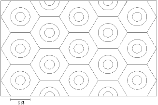
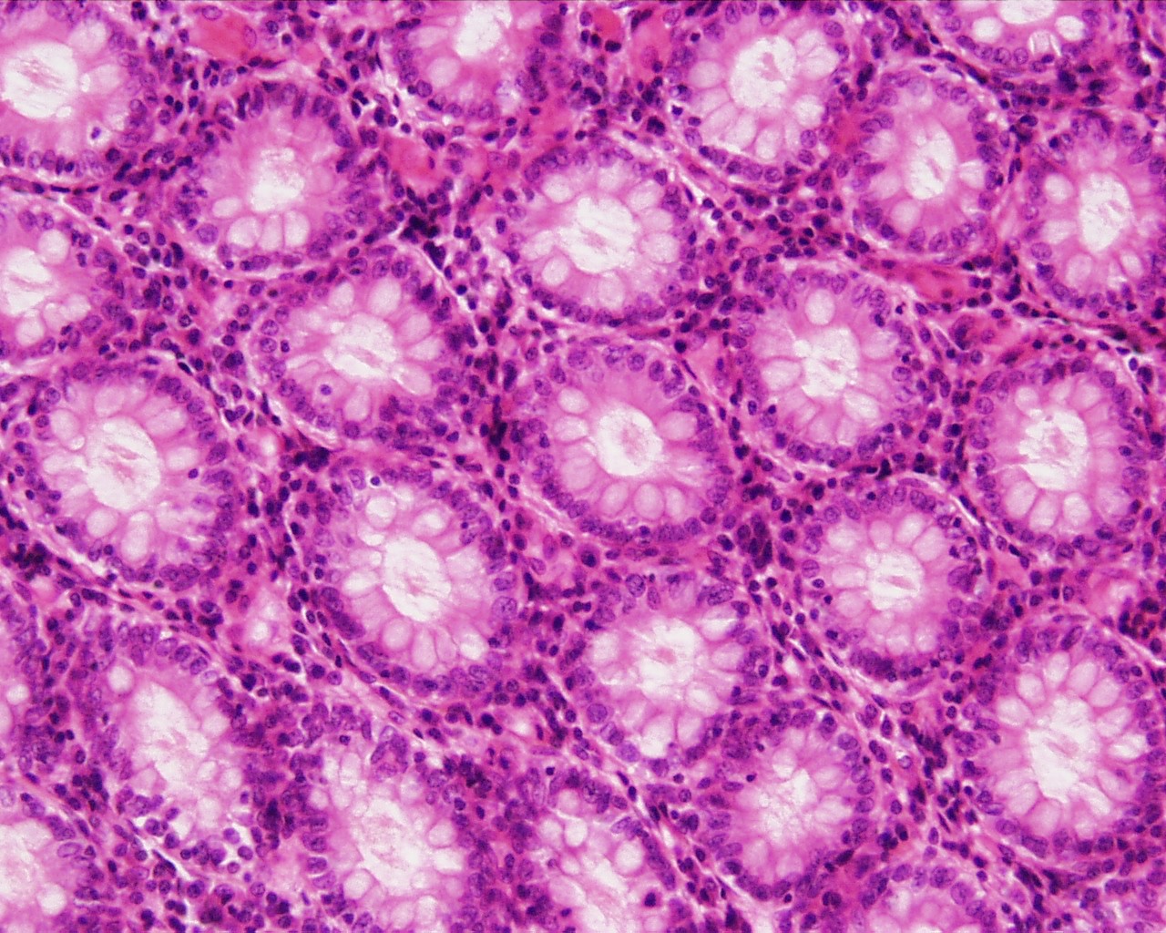
Figure 3: Left image: Two-dimensional and schematic top view of part of the colon wall, considered as an heterogeneous material with a periodic distribution of small heterogeneities, $\varepsilon P$. Each hexagon, with edge of size $\varepsilon a$ represents the region $\varepsilon P$. Inside each hexagon, there is a crypt, containing the colonic cells, and that is represented by the two concentric circles; the region inside the hexagon and outside the large circle is the region surrounding the crypt orifice Right image: Histological image representing a transverse section of the human colon [35]. Compare $\varepsilon P$ with the single region $P$ shown in Figure 2, right.

Therefore we define periodic coefficients $A_{ij}^{\varepsilon},D^{\varepsilon},E^{\varepsilon},\gamma^{\varepsilon},\beta^{\varepsilon}$ (based on the coefficients introduced in (11)) as follows:

$$A_{ij}^{\varepsilon}(X)=A_{ij}\left(\frac{X}{\varepsilon}\right)\quad{\rm and\ }\quad A_{ij}=\left\{\begin{array}[]{l}\mathcal{A}^{*}_{ij}\;\mbox{\ in\ }\;P,\\[5.0pt] \mbox{extended by periodicity (with period $P$) }\\ \mbox{elsewhere in $\mathbb{R}^{2}$,}\end{array}\right.$$

where $X=(X_{1},X_{2})\in\Omega\subset\mathbb{R}^{2}$. Analogous formulae are used for defining the other coefficients $D^{\varepsilon},E^{\varepsilon},\gamma^{\varepsilon},\beta^{\varepsilon}$.

Thus the 2D heterogeneous periodic model, representing the colon epithelium in a 2D setting, corresponds to the following system of two partial differential equations, of elliptic and parabolic type, defined in $\Omega\times]0,T]$, where the unknown is the pair cell density $C^{\varepsilon}$ and pressure $p^{\varepsilon}$.

$$\left\{\begin{array}[]{l}\displaystyle\frac{\partial C^{\varepsilon}}{\partial t}-A_{ij}^{\varepsilon}\frac{\partial}{\partial X_{i}}(C^{\varepsilon}\frac{\partial p^{\varepsilon}}{\partial X_{j}})=A_{ij}^{\varepsilon}\frac{\partial}{\partial X_{i}}(D^{\varepsilon}\frac{\partial C^{\varepsilon}}{\partial X_{j}})+\beta^{\varepsilon}\,C^{\varepsilon}\\ \\ \displaystyle-A_{ij}^{\varepsilon}\frac{\partial^{2}p^{\varepsilon}}{\partial X_{i}\partial X_{j}}=A_{ij}^{\varepsilon}\frac{\partial}{\partial X_{i}}(E^{\varepsilon}\frac{\partial C^{\varepsilon}}{\partial X_{j}})+(\beta^{\varepsilon}-\gamma^{\varepsilon})\,C^{\varepsilon}+\gamma^{\varepsilon}.\end{array}\right.$$ (15)

Homogeneous boundary conditions are assumed for both $C^{\varepsilon}$ and $p^{\varepsilon}$ in $\partial\Omega\times]0,T]$, and the initial condition, at time $t=0$, for the density of abnormal cells is represented by $C^{\varepsilon}(X,0)=C_{0}(X)$. Moreover, compatibility conditions for $t=0$ are hypothesized, that is, $C_{0}(X)=0$ on $\partial\Omega$ and the pressure $p^{\varepsilon}(X,0)$ is the solution to the elliptic equation in (15), when $C^{\varepsilon}$ is replaced by $C_{0}(X)$.

4.2 Two-scale asymptotic expansions

The homogenization technique applied to (15) considers a sequence of problems (15) indexed by $\varepsilon$, and takes the limit of this sequence, when $\varepsilon$ tends to zero. Equivalently, the objective is to find the limit $(C^{0},p^{0})$ of the sequence of solution pairs $\{(C^{\varepsilon},p^{\varepsilon})\}_{\varepsilon>0}$ of (15), in an appropriate topological space. The homogenization model (or equivalently, the limit problem) is the model which has solution $(C^{0},p^{0})$.

Here, we use an heuristic procedure, that consists of forming a two-scale asymptotic expansion in $\varepsilon$ for $C^{\varepsilon}$ and $p^{\varepsilon}$ defined by

$$C^{\varepsilon}(X,t)=\sum_{i=0}^{+\infty}\varepsilon^{i}C^{i}(X,Y,t)\quad\mbox{and }\quad p^{\varepsilon}(X,t)=\sum_{i=0}^{+\infty}\varepsilon^{i}p^{i}(X,Y,t)\qquad(\text{with}\;Y=X/\varepsilon)$$ (16)

in order to formally homogenize the system (15) (see [5, 6, 59] for more details). In this section we identify the limit problem formally.

In (16) $Y=X/\varepsilon$ is the microscopic variable, as opposed to $X$ that is the macroscopic variable. Each term $C^{i}(X,Y,t)$ and $p^{i}(X,Y,t)$ are functions of the variables $X$, $Y$, $t$, and periodic in $Y$ with period $P$.

In what follows, and for the sake of simplifying the computations we always assume that the diffusion coefficients are positive constants that have the same value for normal and abnormal cells. Since there is very little experimental quantitative information about the value of these diffusion coefficients (see [20] for a related work), it is common in the literature to assume that these coefficients are constant and equal [44, 57]. So, from (8) we have

$$D_{N}^{\varepsilon}(Y)=D_{C}^{\varepsilon}(Y)=D>0\,\,\,\,\mbox{and}\,\,\,\,E^{\varepsilon}(Y)=0,\ \forall Y\in P,$$ (17)

and consequently the first term in the second member of the second equation in system (15) disappears.

Then, regarding $X$ and $Y$ as separate variables the differentiation operator $\frac{\partial}{\partial X}$ applied to a function depending on $(X,Y)$ becomes $\frac{\partial}{\partial X}+\frac{1}{\varepsilon}\frac{\partial}{\partial Y}$ and consequently

$$\begin{array}[]{l}\displaystyle\frac{\partial p^{\varepsilon}}{\partial X_{i}}=\displaystyle\frac{1}{\varepsilon}\frac{\partial p^{0}}{\partial Y_{i}}+\Big{(}\frac{\partial p^{0}}{\partial X_{i}}+\frac{\partial p^{1}}{\partial Y_{i}}\Big{)}+\varepsilon\Big{(}\frac{\partial p^{1}}{\partial X_{i}}+\frac{\partial p^{2}}{\partial Y_{i}}\Big{)}+\varepsilon^{2}\Big{(}\frac{\partial p^{2}}{\partial X_{i}}+\frac{\partial p^{3}}{\partial Y_{i}}\Big{)}+\mathcal{O}(\varepsilon^{2})\\ \\ \displaystyle\frac{\partial C^{\varepsilon}}{\partial X_{i}}=\displaystyle\frac{1}{\varepsilon}\frac{\partial C^{0}}{\partial Y_{i}}+\Big{(}\frac{\partial C^{0}}{\partial X_{i}}+\frac{\partial C^{1}}{\partial Y_{i}}\Big{)}+\varepsilon\Big{(}\frac{\partial C^{1}}{\partial X_{i}}+\frac{\partial C^{2}}{\partial Y_{i}}\Big{)}+\varepsilon^{2}\Big{(}\frac{\partial C^{2}}{\partial X_{i}}+\frac{\partial C^{3}}{\partial Y_{i}}\Big{)}+\mathcal{O}(\varepsilon^{2})\end{array}$$ (18)

for $i=1,2$. So, by introducing the two series (16) into the equations (15) and identifying each coefficient of $\varepsilon^{k}$, for $k=-2,-1,0,1,\ldots$ we obtain the following equations for the parabolic equation in (15) :

• The $\varepsilon^{-2}$ equation

  $$-A_{ij}(Y)\left[\frac{\partial C^{0}}{\partial Y_{i}}\frac{\partial p^{0}}{\partial Y_{j}}+C^{0}\frac{\partial^{2}p^{0}}{\partial Y_{i}\partial Y_{j}}\right]=A_{ij}(Y)\left[D\frac{\partial^{2}C^{0}}{\partial Y_{i}\partial Y_{j}}\right].$$ (19)

• The $\varepsilon^{-1}$ equation

  $$\begin{array}[]{rcl}-\displaystyle A_{ij}(Y)\left[\frac{\partial C^{0}}{\partial Y_{i}}\left(\frac{\partial p^{0}}{\partial X_{j}}+\frac{\partial p^{1}}{\partial Y_{j}}\right)+\left(\frac{\partial C^{0}}{\partial X_{i}}+\frac{\partial C^{1}}{\partial Y_{i}}\right)\frac{\partial p^{0}}{\partial Y_{j}}+C^{1}\frac{\partial^{2}p^{0}}{\partial Y_{i}\partial Y_{j}}\right.&+&\\ &&\\ \left.\displaystyle C^{0}\left(\frac{\partial^{2}p^{0}}{\partial X_{i}\partial Y_{j}}+\frac{\partial^{2}p^{0}}{\partial Y_{i}\partial X_{j}}+\frac{\partial^{2}p^{1}}{\partial Y_{i}\partial Y_{j}}\right)\right]&=&\\ &&\\ \displaystyle DA_{ij}(Y)\left(\frac{\partial^{2}C^{0}}{\partial X_{i}\partial Y_{j}}+\frac{\partial^{2}C^{0}}{\partial Y_{i}\partial X_{j}}+\frac{\partial^{2}C^{1}}{\partial Y_{i}\partial Y_{j}}\right).&&\end{array}$$ (20)

• The $\varepsilon^{0}$ equation

  $$\begin{array}[]{rll}\displaystyle\frac{\partial C^{0}}{\partial t}-A_{ij}(Y)\displaystyle\Big{[}\frac{\partial C^{0}}{\partial Y_{i}}\left(\frac{\partial p^{1}}{\partial X_{j}}+\frac{\partial p^{2}}{\partial Y_{j}}\right)+\left(\frac{\partial C^{1}}{\partial X_{i}}+\frac{\partial C^{2}}{\partial X_{j}}\right)\frac{\partial p^{0}}{\partial Y_{j}}+\left(\frac{\partial C^{0}}{\partial X_{i}}+\frac{\partial C^{1}}{\partial Y_{i}}\right)\left(\frac{\partial p^{0}}{\partial X_{j}}+\frac{\partial p^{1}}{\partial Y_{j}}\right)&+&\\ &&\\ \displaystyle C^{0}\left(\frac{\partial^{2}p^{0}}{\partial X_{i}\partial X_{j}}+\frac{\partial^{2}p^{1}}{\partial X_{i}\partial Y_{j}}+\frac{\partial^{2}p^{1}}{\partial Y_{i}\partial X_{j}}+\frac{\partial^{2}p^{2}}{\partial Y_{i}\partial Y_{j}}\right)&+&\\ &&\\ \displaystyle C^{1}\left(\frac{\partial^{2}p^{0}}{\partial X_{i}\partial Y_{j}}+\frac{\partial^{2}p^{0}}{\partial Y_{i}\partial X_{j}}+\frac{\partial^{2}p^{1}}{\partial Y_{i}\partial Y_{j}}\right)+C^{2}\frac{\partial^{2}p^{0}}{\partial Y_{i}\partial Y_{j}}\Big{]}&=&\\ &&\\ D\displaystyle A_{ij}(Y)\left[\frac{\partial^{2}C^{0}}{\partial X_{i}\partial X_{j}}+\frac{\partial^{2}C^{1}}{\partial X_{i}\partial Y_{j}}+\frac{\partial^{2}C^{1}}{\partial Y_{i}\partial X_{j}}+\frac{\partial^{2}C^{2}}{\partial Y_{i}\partial Y_{j}}\right]+\beta(Y)C^{0}.&&\end{array}$$ (21)

And using the same procedure for the elliptic equation in (15) we obtain :

• The $\varepsilon^{-2}$ equation

  $$-A_{ij}(Y)\frac{\partial^{2}p^{0}}{\partial Y_{i}\partial Y_{j}}=0.$$ (22)

• The $\varepsilon^{-1}$ equation

  $$-\displaystyle A_{ij}(Y)\left[\frac{\partial^{2}p^{0}}{\partial X_{i}\partial Y_{j}}+\frac{\partial^{2}p^{0}}{\partial Y_{i}\partial X_{j}}+\frac{\partial^{2}p^{1}}{\partial Y_{i}\partial Y_{j}}\right]=0.$$ (23)

• The $\varepsilon^{0}$ equation

  $$-\displaystyle A_{ij}(Y)\left[\frac{\partial^{2}p^{0}}{\partial X_{i}\partial X_{j}}+\frac{\partial^{2}p^{1}}{\partial X_{i}\partial Y_{j}}+\frac{\partial^{2}p^{1}}{\partial Y_{i}\partial X_{j}}+\frac{\partial^{2}p^{2}}{\partial Y_{i}\partial Y_{j}}\right]=(\beta(Y)-\gamma(Y))C^{0}+\gamma(Y).$$ (24)

Since $p^{0}$ is assumed to be periodic in $Y$ and the coefficients $A_{ij}^{*}$ verify the uniform ellipticity condition (14), we have from (22) that $p^{0}(X,Y)=p^{0}(X)$. So, from (23) we also obtain $p^{1}(X,Y)=p^{1}(X)$. Equation (19) gives $C^{0}(X,Y)=C^{0}(X)$ and consequently (20) yields to $C^{1}(X,Y)=C^{1}(X)$. Finally, these relations permit us to rewrite (24) as the following elliptic equation for $p^{2}$

$$-A_{ij}(Y)\frac{\partial^{2}p^{2}}{\partial Y_{i}\partial Y_{j}}=A_{ij}(Y)\frac{\partial^{2}p^{0}}{\partial X_{i}\partial X_{j}}+(\beta(Y)-\gamma(Y))C^{0}+\gamma(Y).$$ (25)

Using the Fredholm alternative (see for instance [18]), we can assert that problem (25) has solution if, for each $X\in\Omega$

$$\int_{P}[A_{ij}(Y)\frac{\partial^{2}p^{0}}{\partial X_{i}\partial X_{j}}(X)+(\beta(Y)-\gamma(Y))C^{0}+\gamma(Y)]\,m\,dY=0$$ (26)

where $m:\;P\rightarrow\mathbb{R}$ is the unique solution of

$$\left\{\begin{array}[]{l}-\displaystyle\frac{\partial^{2}(A_{ij}m)}{\partial Y_{i}\partial Y_{j}}=0,\\ \\ \mbox{with}\;m\quad P\mbox{-periodic},\;m>0,\;\displaystyle\int_{P}m\,dY=1.\end{array}\right.$$ (27)

Using the notation $\displaystyle\widetilde{f}=\frac{1}{|P|}\int_{P}fdY=\int_{P}fdY$ (because $|P|=1$), for the spatial average of a function $f$ in $P$, the condition (26) has the following form:

$$-\widetilde{A_{ij}m}\frac{\partial^{2}p^{0}}{\partial X_{i}\partial X_{j}}=(\widetilde{\beta m}-\widetilde{\gamma m})C^{0}+\widetilde{\gamma m}\quad\mbox{in}\quad\Omega\times]0,T].$$ (28)

A similar approach can be applied to equation (21), as explained next. Firstly, (24) can be used to rewrite (21) as an elliptic equation for $C^{2}$ in the following way

$$\begin{array}[]{ll}\displaystyle DA_{ij}(Y)\frac{\partial^{2}C^{2}}{\partial Y_{i}\partial Y_{j}}=&\\[5.0pt] \displaystyle\frac{\partial C^{0}}{\partial t}-A_{ij}(Y)\left(\frac{\partial C^{0}}{\partial X_{i}}\frac{\partial p^{0}}{\partial X_{j}}+D\frac{\partial^{2}C^{0}}{\partial X_{i}\partial X_{j}}\right)-(\beta(Y)-\gamma(Y))C^{0}(1-C^{0}).\end{array}$$ (29)

Since $D$ is a positive constant and using again the Fredholm alternative, we have that (29) has a solution if, for all $X\in\Omega$ the equation

$$\int_{P}\left[\frac{\partial C^{0}}{\partial t}-A_{ij}(Y)\left(\frac{\partial C^{0}}{\partial X_{i}}\frac{\partial p^{0}}{\partial X_{j}}+D\frac{\partial^{2}C^{0}}{\partial X_{i}\partial X_{j}}\right)-(\beta(Y)-\gamma(Y))C^{0}(1-C^{0})\right]mdY=0$$ (30)

is verified, where $m$ is again the solution of (27). Since $C^{0}=C^{0}(X)$ and $p^{0}=p^{0}(X)$, therefore (30) can be rewritten as follows

$$\frac{\partial C^{0}}{\partial t}-\widetilde{A_{ij}m}\frac{\partial C^{0}}{\partial X_{i}}\frac{\partial p^{0}}{\partial X_{j}}=D\widetilde{A_{ij}m}\frac{\partial^{2}C^{0}}{\partial X_{i}\partial X_{j}}+(\widetilde{\beta m}-\widetilde{\gamma m})C^{0}(1-C^{0}).$$ (31)

In conclusion, the (formal) homogenization model defined in $\Omega\times]0,T]$, and resulting from the heterogeneous periodic model (15), is the following system

$$\left\{\begin{array}[]{l}\displaystyle\frac{\partial C^{0}}{\partial t}-\widetilde{A_{ij}m}\frac{\partial C^{0}}{\partial X_{i}}\frac{\partial p^{0}}{\partial X_{j}}=D\widetilde{A_{ij}m}\frac{\partial^{2}C^{0}}{\partial X_{i}\partial X_{j}}+(\widetilde{\beta m}-\widetilde{\gamma m})C^{0}(1-C^{0})\\ \\ -\displaystyle\widetilde{A_{ij}m}\frac{\partial^{2}p^{0}}{\partial X_{i}\partial X_{j}}=(\widetilde{\beta m}-\widetilde{\gamma m})C^{0}+\widetilde{\gamma m}\end{array}\right.$$ (32)

whose unknown is the pair $(C^{0},p^{0})$. This is a macroscopic model that represents the evolution of ACF at the surface of the colon, by using the information of the cell dynamics in the crypts. This information is transmitted to the homogenization model through the physiologic parameters that in (32) are averaged (they are represented by the same letters as before with a tilde over them).

5 Existence of solution to the homogenization model

5.1 Some Banach spaces and corresponding norms

We denote by $X_{i}$, with $i=1,2$, the components of a generic point $X=(X_{1},X_{2})\in\Omega$ and by $D_{X_{i}}$ the partial derivative with respect to $X_{i}$. For $\alpha\in]0,1[$ and $T>0$ fixed, we consider the Banach spaces $C^{\alpha}(\overline{\Omega})$ and $C^{\alpha}(\overline{\Omega}_{T})$, where $\overline{\Omega}_{T}=\overline{\Omega}\times[0,T]$, endowed with the norms (see for instance [52])

$$\|u\|_{C^{\alpha}(\overline{\Omega})}=\sup_{X\in\overline{\Omega}}|u(X)|+\sup_{X,Y\in\overline{\Omega}}\frac{|u(X)-u(Y)|}{|X-Y|^{\alpha}}$$

and

$$\|u\|_{C^{\alpha}(\overline{\Omega}_{T})}=\sup_{(X,t)\in\overline{\Omega}_{T}}|u(X,t)|+\sup_{(X,t),(\xi,\tau)\in\overline{\Omega}_{T}}\displaystyle\frac{|u(X,t)-u(\xi,\tau)|}{(|t-\tau|+|X-\xi|^{2})^{\frac{\alpha}{2}}}.$$

We denote by $H^{1+\alpha,\alpha}(\overline{\Omega}_{T})$ the space

$$H^{1+\alpha,\alpha}(\overline{\Omega}_{T})=\left\{u:\overline{\Omega}_{T}\longrightarrow\mathbb{R}\;\Big{|}\quad u,\;D_{X_{i}}u\in C^{\alpha}(\overline{\Omega}_{T}),\;\|u\|_{H^{1+\alpha,\alpha}(\overline{\Omega}_{T})}<\infty\right\}$$

equipped with the norm

$$\begin{array}[]{lcl}\|u\|_{H^{1+\alpha,\alpha}(\overline{\Omega}_{T})}&=&\displaystyle\sup_{(X,t)\in\overline{\Omega}_{T}}|u(X,t)|\;+\displaystyle\sup_{(X,t),(X,t^{\prime})\in\overline{\Omega}_{T}}\frac{|u(X,t)-u(X,t^{\prime})|}{|t-t^{\prime}|^{\frac{\alpha}{2}}}\\ &&\\ &+&\displaystyle\sum_{i=1,2}\left(\sup_{(X,t)\in\overline{\Omega}_{T}}|D_{X_{i}}u(X,t)|+\sup_{(X,t),(Y,t)\in\overline{\Omega}_{T}}\frac{|D_{X_{i}}u(X,t)-D_{X_{i}}u(Y,t)|}{|X-Y|^{\alpha}}\right.\\ &&\\ &+&\left.\displaystyle\sup_{(X,t),(X,t^{\prime})\in\overline{\Omega}_{T}}\frac{|D_{X_{i}}u(X,t)-D_{X_{i}}u(X,t^{\prime})|}{|t-t^{\prime}|^{\frac{\alpha}{2}}}\right).\end{array}$$ (33)

We remark that $H^{1+\alpha,\alpha}(\overline{\Omega}_{T})$ is a Banach space (see for example [27, p. 795], where it is proven that $H^{1+\alpha,\alpha}(\overline{\Omega}_{T})$ is a Banach space, when endowed with a norm equivalent to that defined in (33)).

Moreover, if $V$ is a Banach space, we also consider the set

$$\mathcal{C}^{\alpha}([0,T];V)=\left\{u:[0,T]\longrightarrow V\;\left|\quad\frac{\|f(t+h)-f(t)\|_{V}}{|t-s|^{\alpha}}<M,\quad\forall t,t+h\in[0,T]\right.\right\}.$$

where $M$ is a constant. This space is also a Banach space when equipped with the norm

$$\|u\|_{\mathcal{C}^{\alpha}([0,T];V)}=\sup_{t\in[0,T]}\|u(t)\|_{V}+\sup_{s,t\in[0,T]}\frac{\|u(t)-u(s)\|_{V}}{|t-s|^{\alpha}}.$$ (34)

In addition we also consider the following two spaces (see for example [19]):

- the space $C^{1,\alpha}(\overline{\Omega})$ consisting of those functions $u:\Omega\rightarrow\mathbb{R}$ that are one-time continuously differentiable and whose first-partial derivatives are Hölder continuous with exponent $\alpha$.

- the Sobolev space $W^{2,q}(\Omega)$, for $q\geq 1$, consisting of all locally summable functions $u:\Omega\rightarrow\mathbb{R}$, whose weak partial derivatives, up to the order $2$, exist and belong to $L^{q}(\Omega)$.

5.2 Partial existence results

The two following lemmas assure the existence and uniqueness of solutions of the parabolic and elliptic equations (32), separately. These results will be used in the next section for proving the existence of solution of the homogenized system (32).

In what follows we will assume that the domain $\Omega$ is sufficiently regular to be able to use the known results on a priori estimates for the solution of elliptic and semilinear parabolic problems.

Lemma 5.1.

Let $W\in\left(C^{\alpha}(\overline{\Omega}_{T})\right)^{2}$ and consider the semilinear parabolic problem

$$\left\{\begin{array}[]{lcl}\displaystyle\frac{\partial C}{\partial t}-LC=f(X,t,C),&\mbox{in}&\Omega\times]0,T]\\ &&\\ C=0,&\mbox{on}&\partial\Omega\times]0,T]\\ &&\\ C(X,0)=C_{0}(X)&\mbox{in}&\Omega\times\{0\}\end{array}\right.$$ (35)

where $L:=\widetilde{A_{ij}m}W\frac{\partial}{\partial X_{i}}+D\widetilde{A_{ij}m}\frac{\partial^{2}}{\partial X_{i}\partial X_{j}}$ , $f(X,t,C):=(\widetilde{\beta m}-\widetilde{\gamma m})C(1-C)$ and the initial condition $C_{0}\in C^{\alpha}(\overline{\Omega})$ satisfies $C_{0}(X)_{|_{\partial\Omega}}=0$ with $0\leq C_{0}(X)\leq 1$. Then,

1. Problem (35) has an unique solution $C$, such that:

   $$0\leq C(X,t)\leq 1,\quad\forall(X,t)\in\overline{\Omega}_{T}.$$

2. If the initial condition $C_{0}$ is regular enough and verifies $C=0$ on $\partial\Omega$, then $C\in H^{1+\alpha,\alpha}(\overline{\Omega}_{T})$ and if $(\widetilde{\beta m}-\widetilde{\gamma m})$ is small enough, there exists a positive constant $M$ such that

   $$\|C\|_{H^{1+\alpha,\alpha}(\overline{\Omega}_{T})}\leq M.$$

Proof: The first statement is a direct consequence of [52, Theorem 5.1, p. 66]. Concerning the second statement, we use [28, Theorem 8, p. 204]. The hypotheses of this lemma for the domain, initial condition and coefficients are the same as those used in [28, Theorem 8, p. 204], but for this latter theorem there is the following extra requirement for $f(.,.)$ in (35) that should be fulfilled :

$$2K|f(X,t,C)|\leq M\quad\mbox{in }\quad\Omega_{T}$$ (36)

(where $|.|$ represents the modulus) for all $C\in H^{1+\alpha,\alpha}(\overline{\Omega}_{T})$, with $\|C\|_{H^{1+\alpha,\alpha}(\overline{\Omega}_{T})}<M$, where $K$ is a constant depending on $\alpha$, $\Omega_{T}$ and on the coefficients of the convective term of the parabolic operator. Due the particular form of the function $f$, in our case, we can conclude the condition (36) is satisfied if $(\widetilde{\beta m}-\widetilde{\gamma m})$ is sufficiently small. $\Box$

Lemma 5.2.

For a given $C\in C^{\alpha}(\overline{\Omega}_{T})$ and for each $t\in[0,T]$ the elliptic problem

$$\left\{\begin{array}[]{lcl}\displaystyle-(\widetilde{A_{ij}m})\frac{\partial^{2}p}{\partial X_{i}\partial X_{j}}=(\widetilde{\beta m}-\widetilde{\gamma m})C+\widetilde{\gamma m},&\mbox{in}&\Omega\times[0,T]\\ &&\\ p=0,&\mbox{on}&\partial\Omega\times[0,T]\end{array}\right.$$ (37)

has an unique solution $p$ in $\mathcal{C}^{\frac{\alpha}{2}}([0,T];W^{2,q}(\Omega))$, for $q>2$. Furthermore

$$\|p\|_{\mathcal{C}^{\frac{\alpha}{2}}([0,T];W^{2,q}(\Omega))}\leq M$$ (38)

where $M$ is a constant that depends on $\|C\|_{C^{\alpha}(\overline{\Omega}_{T})}$.

Proof: Using regularity results and a priori estimates for second order elliptic equations (see for instance [52, p. 95]) and the regularity of $C$ we conclude that, for each fixed $t\in[0,T]$, the solution $p$ of (37) is in $W^{2,q}(\Omega)$ with $q>2$ and

$$\|p\|_{W^{2,q}(\Omega)}\leq M\|(\widetilde{\beta m}-\widetilde{\gamma m})C+\widetilde{\gamma m}\|_{L^{p}(\Omega)}$$ (39)

where $M$ is a constant independent of $t$. Thus, using the regularity of $C$, we have

$$\|p\|_{W^{2,q}(\Omega)}\leq M$$ (40)

where $M>0$ is another constant independent of $t$ and depending on $C$, which can be small if $\|\widetilde{\gamma m}\|_{L^{p}(\Omega)}$ and $\|\widetilde{\beta m}-\widetilde{\gamma m}\|_{L^{p}(\Omega)}$ are sufficiently small.

Considering now (37) for two different times $t=t_{1}$ and $t=t_{2}$, subtracting the two corresponding equations and dividing by $|t_{1}-t_{2}|^{\alpha}$, we obtain

$$-(\widetilde{A_{ij}m})\frac{\partial^{2}}{\partial X_{i}\partial X_{j}}\left(\frac{p(t_{1})-p(t_{2})}{|t_{1}-t_{2}|^{\alpha}}\right)=(\widetilde{\beta m}-\widetilde{\gamma m})\left(\frac{C(X,t_{1})-C(X,t_{2})}{|t_{1}-t_{2}|^{\alpha}}\right),\,\,\,\,\,\mbox{in}\,\,\,\,\Omega\times[0,T].$$

Then, using the same argument as the beginning of this proof, we have

$$\left\|\frac{p(t_{1})-p(t_{2})}{|t_{1}-t_{2}|^{\alpha}}\right\|_{W^{2,q}(\Omega)}\leq M$$ (41)

where $M$ is another constant, depending on $\gamma$, but independent of $t$. From (40)-(41) we have $p\in\mathcal{C}^{\frac{\alpha}{2}}([0,T];W^{2,p}(\Omega))$ and also

$$||p||_{\mathcal{C}^{\frac{\alpha}{2}}([0,T];W^{2,q}(\Omega))}\leq M.\qquad\Box$$ (42)

Remark 5.1.

We observe that from (39)-(42) we can conclude that, for each $C\in{C^{\alpha}(\overline{\Omega}_{T})}$, such that $\|C\|_{C^{\alpha}(\overline{\Omega}_{T})}\leq K$, with $K$ constant, then the norm $\|p\|_{\mathcal{C}^{\frac{\alpha}{2}}([0,T],W^{2,p}(\Omega))}$ can be arbitrarily small by taking $\widetilde{\gamma m}$ and $\widetilde{\beta m}-\widetilde{\gamma m}$ sufficiently small.

5.3 Main existence result

Using a fixed-point type argument we can prove the existence of a solution to the homogenization model (32).

Theorem 5.1.

Let $\Omega$ be an open and bounded domain in $\mathbb{R}^{2}$ with boundary $\partial\Omega$ regular enough, $T$ a fixed positive real number and $(\widetilde{\gamma m})$, $(\widetilde{\beta m}-\widetilde{\gamma m})$ sufficiently small. Then, the homogenization model (32) has a solution $(C^{0},p^{0})$ such that $p^{0}\in C^{\frac{\alpha}{2}}([0,T];C^{1,\alpha}(\overline{\Omega}))$ and $C^{0}\in C^{\alpha}(\overline{\Omega}_{T})$.

Proof: The proof is based on Schauder’s fixed point theorem (see for instance [19]). So the goal is to define an appropriate continuous operator $\mathcal{F}$ in a compact and convex subset $K$ of a Banach space, such that $\mathcal{F}:K\rightarrow K$, which implies that $\mathcal{F}$ has a fixed point.

Thus we first consider an operator $S$ defined in the domain

$$B_{M}(0)=\{v\in C^{\alpha}(\overline{\Omega}_{T}):v(X,0)=C_{0}(X)\,\,\,\mbox{and}\,\,\,||v||_{C^{\alpha}(\overline{\Omega}_{T})}\leq M\}$$ (43)

with $M$ a fixed constant and $C_{0}$ the initial condition in (35). We prove in the following that $\mathcal{F}:B_{M}(0)\rightarrow B_{M}(0)$, defined as $\mathcal{F}=Q\circ G\circ D\circ I\circ E$, verifies Schauder’s fixed point theorem.

• $E$ is the continuous operator defined by

  $$\begin{array}[]{lccl}E:&B_{M}(0)&\longrightarrow&\mathcal{C}^{\frac{\alpha}{2}}([0,T];W^{2,q}(\Omega))\\ &C&\longmapsto&p\end{array}$$ (44)

  where $q>2$. The image $p=E(C)$ is the solution of the elliptic problem (37), given by Lemma 5.2.

• $I$ is an inclusion, that identifies $p=E(C)\in C^{\frac{\alpha}{2}}([0,T];W^{2,q}(\Omega))$ with $p\in C^{\frac{\alpha}{2}}([0,T];C^{1,\alpha}(\overline{\Omega}))$. The Sobolev embedding theorem (see for instance [19, p. 270]) guarantees the continuity of $I$.

• $D$ is an operator that applies each $p\in\mathcal{C}^{\frac{\alpha}{2}}([0,T];C^{1,\alpha}(\overline{\Omega}))$ in $\hat{p}\in H^{1+\alpha,\alpha}(\overline{\Omega}_{T})$ defined by

  $$\begin{array}[]{lccl}\hat{p}:&\overline{\Omega}_{T}&\longrightarrow&\mathbb{R}\\ &(X,t)&\longmapsto&\hat{p}(X,t)=p(t)(X).\end{array}$$ (45)

  We can easily conclude, using the norms (33) and (34) that there exist a constant $M>0$ such that

  $$||\hat{p}||_{H^{1+\alpha,\alpha}(\overline{\Omega}_{T})}\leq M||p||_{\mathcal{C}^{\frac{\alpha}{2}}([0,T];C^{1,\alpha}(\overline{\Omega}))}.$$ (46)

• $G$ is the gradient operator defined by

  $$\begin{array}[]{lccl}G:&H^{1+\alpha,\alpha}(\overline{\Omega}_{T})&\longrightarrow&\left(C^{\alpha}(\overline{\Omega}_{T})\right)^{2}\\[5.0pt] &\hat{p}&\longmapsto&\nabla\hat{p}=\displaystyle\left(\frac{\partial\hat{p}}{\partial X_{1}},\frac{\partial\hat{p}}{\partial X_{2}}\right).\end{array}$$ (47)

  Using the definitions of the $C^{\alpha}(\overline{\Omega})$ and $H^{1+\alpha,\alpha}(\overline{\Omega}_{T})$ norms, we deduce the continuity of $G$

  $$\Big{\|}\frac{\partial\hat{p}}{\partial X_{i}}\Big{\|}_{C^{\alpha}(\overline{\Omega})}\leq\|\hat{p}\|_{H^{1+\alpha,\alpha}(\overline{\Omega}_{T})}.$$

• $Q$ is the operator that applies each $W\in(C^{\alpha}(\overline{\Omega}_{T}))^{2}$ in $Q(W)\in C^{\alpha}(\overline{\Omega}_{T})$, that is the solution of the semilinear parabolic problem (35), given in Lemma 5.1. $Q$ is a continuous operator when restricted to $G\circ D\circ I\circ E(B_{M}(0))$. In fact, if $W^{n}:=(W_{1}^{n},W_{2}^{n})$ is a sequence that convergences to $W:=(W_{1},W_{2})$ in $(C^{\alpha}(\overline{\Omega}_{T}))^{2}$, when $n\rightarrow\infty$, then also the corresponding images by the operator $Q$ converge, that is,

  $$C^{n}:=Q\big{(}(W_{1}^{n},W_{2}^{n})\big{)}\longrightarrow C:=Q\big{(}(W_{1},W_{2})\big{)}\quad\mbox{in}\;C^{\alpha}(\overline{\Omega}_{T}),\;\mbox{when}\;n\rightarrow\infty.$$

  This statement can be proved using a priori estimates for linear parabolic problems. In effect, defining $U^{n}=C^{n}-C$ and

  $$f^{n}(X,t)=(\widetilde{\beta m}-\widetilde{\gamma m})U^{n}(1-(C^{n}+C))+\widetilde{A_{ij}m}(W^{n}-W)\frac{\partial C^{n}}{\partial X_{i}}$$

  it can be derived (easily) that $U^{n}$ is the solution of

  $$\left\{\begin{array}[]{lcl}\displaystyle\frac{\partial U^{n}}{\partial t}-\widetilde{A_{ij}m}W\frac{\partial U^{n}}{\partial X_{i}}-D\widetilde{A_{ij}m}\frac{\partial^{2}U^{n}}{\partial X_{i}\partial X_{j}}=f^{n}(X,t)&\mbox{in}&\Omega\times]0,T]\\ \\ U^{n}=0&\mbox{on}&\partial\Omega\times]0,T]\\ \\ U^{n}(X,0)=0&\mbox{in}&\Omega\times\{0\}.\end{array}\right.$$ (48)

  As $f^{n}$ verifies the hypotheses of [28, Theorems 6 and 7, p. 65], then the next estimate for $\|U^{n}\|_{C^{\alpha}(\overline{\Omega}_{T})}$ is valid

  $$\|U^{n}\|_{C^{\alpha}(\overline{\Omega}_{T})}\leq\Big{\|}(\widetilde{\beta m}-\widetilde{\gamma m})U^{n}(1-(C^{n}+C))+\widetilde{A_{ij}m}(W^{n}-W)\frac{\partial C^{n}}{\partial X_{i}}\Big{\|}_{C^{\alpha}(\overline{\Omega}_{T})}.$$

  Moreover since $\|C\|_{C^{\alpha}(\overline{\Omega}_{T})}$, $\|C^{n}\|_{C^{\alpha}(\overline{\Omega}_{T})}$ and $\|\frac{\partial C^{n}}{\partial X_{i}}\|_{C^{\alpha}(\overline{\Omega}_{T})}$ are bounded we can conclude that for some constant $K_{1}$, the following relation is valid

  $$\|C^{n}-C\|_{C^{\alpha}(\overline{\Omega}_{T})}=\|U^{n}\|_{C^{\alpha}(\overline{\Omega}_{T})}\leq K_{1}\left(|(\widetilde{\beta m}-\widetilde{\gamma m})|\|C^{n}-C\|_{C^{\alpha}(\overline{\Omega}_{T})}+\|(W^{n}-W)\|_{C^{\alpha}(\overline{\Omega}_{T})}\right).$$

  Supposing that $|(\widetilde{\beta m}-\widetilde{\gamma m})|$ is small enough we obtain

  $$\|C^{n}-C\|_{C^{\alpha}(\overline{\Omega}_{T})}\leq K_{2}\|(W^{n}-W)\|_{C^{\alpha}(\overline{\Omega}_{T})}$$

  where $K_{2}$ is another constant. This proves the sequential continuity and consequently the continuity of $Q$.

Finally, for $M>0$ and with the conditions of [28, Theorem 8, p.204], we must show that $\mathcal{F}(B_{M}(0))\subset B_{M}(0)$, in order to apply Schauder’s fixed point theorem. As $G\circ D\circ I$ is a linear continuous operator, then

$$\|G\circ D\circ I\big{(}E(C)\big{)}\|_{(C^{\alpha}(\overline{\Omega}_{T}))^{2}}\leq K_{3}\|E(C)\|_{C^{\frac{\alpha}{2}}([0,T];C^{1,\alpha}(\overline{\Omega}))}$$ (49)

with $K_{3}$ a continuity constant. Taking into account Remark 5.1, the second term of (49) can be chosen arbitrarily small. In this way, it is possible to obtain the right upper bound for the coefficients of the convective term of the parabolic operator, see (36), and consequentely Lemma 5.1 ensures that $\mathcal{F}(C)\in B_{M}(0)$. Therefore the solution of the homogenization model (32) is a fixed point of $\mathcal{F}$. $\Box$

6 Approximate solution of the homogenization model

In this section, a numerical approach to solve the homogenized system (32) is briefly described. The space-time discretization is based on continuous finite elements for the space variable, and finite differences (using an implicit backward Euler scheme) for the time variable.

The variational formulation corresponding to the elliptic equation in (32) is

$$\int_{\Omega}\widetilde{A_{ij}m}\frac{\partial p^{0}}{\partial X_{j}}\frac{\partial v}{\partial X_{i}}dX_{1}dX_{2}=\int_{\Omega}[(\widetilde{\beta m}-\widetilde{\gamma m})\,C^{0}+\widetilde{\gamma m}]\,vdX_{1}dX_{2},\,\,\,\,\,\,\forall v\in H_{0}^{1}(\Omega).$$ (50)

Then, denoting by $\{\varphi_{k}\}$ the global finite element shape functions, and considering a partition in the time interval $[0,T]$, such that $[0,T]=\cup_{n=0}^{N-1}[t_{n},t_{n+1}]$ with time step size $\Delta t=t_{n+1}-t_{n}$, (50) leads to the following approximation of the homogenized elliptic problem

$$\widetilde{G}_{m}{\bf p^{n}}=(\widetilde{\beta m}-\widetilde{\gamma m})\,M\,{\bf C^{n}}\,+\,{\bf\widetilde{\boldsymbol{\gamma m}}}.$$ (51)

Here ${\bf p^{n}}=(p_{k}^{n})$ and ${\bf C^{n}}=(C_{k}^{n})$ are vectors, corresponding to the space-time discretizations of $p^{0}$ and $C^{0}$, respectively (${\bf C^{n}}$ depends explicitly and ${\bf p^{n}}$ implicitly on the time variable $t$). The upper index ($\bf n$ for vector and $n$ for vector component) corresponds to the approximation at time $t_{n}$ and the lower index $k$ to the finite element node number considered. Finally, $M$ and $\widetilde{G}$ are, respectively, the finite element mass matrix and modified stiffness matrix and ${\bf\widetilde{\boldsymbol{\gamma m}}}=(\widetilde{\gamma m}_{k})$ is a vector, defined by

$$\begin{array}[]{lcl}{\bf\widetilde{\boldsymbol{\gamma m}}}=(\widetilde{\gamma m}_{k})&&\widetilde{\gamma m}_{k}:=\displaystyle\int_{\Omega}\widetilde{\gamma m}\,\varphi_{k}dX_{1}dX_{2},\\ \\ M=(M_{k,l})&&M_{k,l}:=\displaystyle\int_{\Omega}\varphi_{k}\varphi_{l}dX_{1}dX_{2},\\ \\ \widetilde{G}_{m}=(\widetilde{G}_{k,l})&&\widetilde{G}_{k,l}:=\displaystyle\int_{\Omega}\nabla\varphi_{k}\cdot(\widetilde{Am}\nabla\varphi_{l})dX_{1}dX_{2},\end{array}$$ (52)

with $\widetilde{Am}=\left(\widetilde{A_{ij}m}\right)_{i,j=1,2}$.

We can use similar arguments for approximating the parabolic equation in (32). Its variational formulation is

$$\begin{array}[]{l}\displaystyle\int_{\Omega}\left(\frac{\partial C^{0}}{\partial t}-\widetilde{A_{ij}m}\frac{\partial C^{0}}{\partial X_{i}}\frac{\partial p^{0}}{\partial X_{j}}\right)\,v\,dX_{1}dX_{2}=\\ \\ \displaystyle\int_{\Omega}\left(-D\widetilde{A_{ij}m}\frac{\partial C^{0}}{\partial X_{j}}\frac{\partial v}{\partial X_{i}}+(\widetilde{\beta m}-\widetilde{\gamma m})C^{0}(1-C^{0})\,v\right)\,dX_{1}dX_{2},\quad\forall v\in H_{0}^{1}(\Omega).\end{array}$$ (53)

It involves, in particular, a bilinear term in $C^{0}$ and $p^{0}$ and a non-linear term in $C^{0}$. For the bilinear term we remark that at time $t_{n}$

$$\begin{array}[]{lcl}\displaystyle\int_{\Omega}\widetilde{A_{ij}m}\frac{\partial C^{0}}{\partial X_{i}}\frac{\partial p^{0}}{\partial X_{j}}v\,dX_{1}dX_{2}&=&\displaystyle\int_{\Omega}\frac{\partial C^{0}}{\partial X_{i}}(\widetilde{Am}\nabla p^{0})_{i}v\,dX_{1}dX_{2}\\ \\ &\simeq&\displaystyle\sum_{s,l}p_{s}^{n}C_{l}^{n}\int_{\Omega}(\nabla\varphi_{l}\cdot\widetilde{Am}\nabla\varphi_{s})v\,dX_{1}dX_{2},\end{array}$$ (54)

and then, using $v=\varphi_{k}$ we have

$$\int_{\Omega}\widetilde{A_{ij}m}\frac{\partial C^{0}}{\partial X_{i}}\frac{\partial p^{0}}{\partial X_{j}}\varphi_{k}\,dX_{1}dX_{2}\simeq(\widetilde{D}_{m,\nabla p}{\bf C^{n}})_{k}$$

where

$$(\widetilde{D}_{m,\nabla p})_{k,l}:=\displaystyle\sum_{s}p_{s}^{n}\int_{\Omega}\nabla\varphi_{l}\cdot\widetilde{Am}\nabla\varphi_{s}\,\varphi_{k}\,dX_{1}dX_{2}.$$ (55)

Using a backward Euler discretization in time with time step size $\Delta t$, the variational formulation (53) is approximated by the equation

$$M\frac{{\bf C^{n+1}}-{\bf C^{n}}}{\Delta t}-\widetilde{D}_{m,\nabla p}{\bf C^{n+1}}=-\widetilde{G}_{m,D}{\bf C^{n+1}}+\Big{[}M_{\widetilde{\beta m}-\widetilde{\gamma m}}({\bf 1}-{\bf C^{n}})\Big{]}{\bf C^{n+1}}$$ (56)

where the last term in the right hand side corresponds to the approximation of the non-linear term $(1-C^{0})C^{0}$ (by using $({\bf 1}-{\bf C^{n}})$ and ${\bf C^{n+1}}$ for approximating $(1-C^{0})$ and $C^{0}$, at time $t_{n}$ and $t_{n+1}$, respectively). In (56)

$$\begin{array}[]{lcl}M_{\widetilde{\beta m}-\widetilde{\gamma m}}({\bf 1}-{\bf C^{n}})=(M_{k,l})&&M_{k,l}:=\displaystyle\int_{\Omega}({\widetilde{\beta m}-\widetilde{\gamma m}})\,(1-C_{s}^{n})\varphi_{s}\,\varphi_{k}\,\varphi_{l}\,dX_{1}dX_{2},\\ \\ \widetilde{G}_{m,D}=(\widetilde{G}_{k,l})&&\widetilde{G}_{k,l}:=\displaystyle\int_{\Omega}D\nabla\varphi_{k}\cdot(\widetilde{Am}\nabla\varphi_{l})dX_{1}dX_{2},\end{array}$$ (57)

are other modified mass and stiffness finite element matrices. With a such approximation the parabolic equation can be solved by computing $\bf C^{n+1}$ at each time step $t_{n+1}$, by solving the linear system

$$\Big{(}M+\Delta t\big{(}-\widetilde{D}_{m,\nabla p}+\widetilde{G}_{m,D}-M_{\widetilde{\beta m}-\widetilde{\gamma m}}(1-{\bf C^{n}})\big{)}\Big{)}{\bf C^{n+1}}=M{\bf C^{n}}.$$ (58)

Summarizing, the algorithm implemented in the time interval $[0,T]$, with time step size $\Delta t=t_{n+1}-t_{n}$, and the initial condition ${\bf C^{0}}$ (for the density of abnormal cells) is listed below.

• Compute ${\bf p^{0}}$ the approximation of the pressure at time $t=0$, by using (51), i.e.

  $$\widetilde{G}_{m}{\bf p^{0}}=(\widetilde{\beta m}-\widetilde{\gamma m})\,M\,{\bf C^{0}}\,+\,\widetilde{\bf{\boldsymbol{\gamma m}}}$$

  and set $n=0$.

• While $t_{n}<T$

  1. Build the matrix $\widetilde{D}_{m,\nabla p}$ defined in (55), for ${\bf p^{n}}$, i.e

     $$(\widetilde{D}_{m,\nabla p})_{k,l}:=\displaystyle\sum_{s}p_{s}^{n}\int_{\Omega}\nabla\varphi_{l}\cdot\widetilde{Am}\nabla\varphi_{s}\,\varphi_{k}\,dX_{1}dX_{2}.$$

  2. Compute $\bf C^{n+1}$ using the backward Euler equation (58) with $\widetilde{D}_{m,\nabla p}$ computed in the previous step 1, i.e

     $$\Big{(}M+\Delta t\big{(}-\widetilde{D}_{m,\nabla p}+\widetilde{G}_{m,D}-M_{\widetilde{\beta m}-\widetilde{\gamma m}}(1-{\bf C^{n}})\big{)}\Big{)}{\bf C^{n+1}}=M{\bf C^{n}}.$$

  3. Compute $\bf p^{n+1}$ using (51), i.e.

     $$\widetilde{G}_{m}{\bf p^{n+1}}=(\widetilde{\beta m}-\widetilde{\gamma m})\,M\,{\bf C^{n+1}}\,+\,{\bf\widetilde{\boldsymbol{\gamma m}}}.$$

  4. Increment $n$, that is $n=n+1$, and go to step 1.

• Stop when $t_{n}=T$.

7 Numerical simulations

In this section we present the numerical simulations for the homogenized model (32), obtained by implementing the algorithm described in the previous Section 6. Moreover we compare these results with those obtained by solving numerically the heterogeneous problem (15).

The crypt geometry is related to the real dimensions of colonic crypts: the domain, representing a piece of the colon, is $\Omega=[-1,1]\times[-1,1]$ (a rectangle as well could have been considered, as shown in Figure 3) and the values for the radius of the shrunk crypt bottom, the radius of the top crypt orifice and the crypt height, in (1)-(2), are $r=a/4$, $R=a/2$ and $L=14a$, respectively, where $a=\frac{\sqrt{2}}{3^{\frac{3}{4}}}$ is the edge of the reference hexagon $P$ of area 1. We have used the relation $L/2R=14$, between the dimensions of the height $L$ and the diameter $2R$, according to the dimensions reported for human colonic crypts in [32, 33] ($433\,\mu m$ for the crypt height, $16\,\mu m$ for the crypt top orifice excluding the epithelium and $15.1\mu m$ for the epithelium cell depth). The time unit measure used is the hour. Triangular finite elements and 3-point Gaussian quadrature rule are used for the finite element discretization used to get $m$ that satisfies (27) in $P$. Bilinear finite elements and 4-point Gaussian quadrature rule are used for the finite element discretization of the systems (15) and (32).

Concerning the values for the parameters, we define the proliferative coefficients $\gamma$ and $\beta$, introduced in (6), by

$$\begin{array}[]{lcl}\gamma(x_{3})&=&\left\{\begin{array}[]{cl}\tau_{\gamma}(x_{3}-2/3L)^{2}&{\rm if}\quad x_{3}\leq\frac{2}{3}L\\[2.5pt] 0&{\rm elsewhere}\end{array}\right.\\ \\ \beta(x_{3})&=&\left\{\begin{array}[]{cl}\tau_{\beta_{1}}(x_{3}-2/3L)^{2}+\beta_{2}&{\rm if}\quad x_{3}\leq\frac{2}{3}L\\[2.5pt] \beta_{2}&{\rm elsewhere}\end{array}\right.\end{array}$$ (59)

with $\tau_{\gamma}=\tau_{\beta_{1}}=0.01$, $\beta_{2}=0.1$. This choice reassures the known qualitative behavior of colonic cells to have a high proliferation at the bottom of the crypt (where $x_{3}=0$) that decreases going upwards to the orifice (where $x_{3}=L$) along the crypt axis, see [23]. Moreover, as assumed by several authors (see for instance [16, 38]) we suppose that there is no proliferation in the last third of the crypt (starting from the bottom), that is for $x_{3}\geq\frac{2}{3}L$. We use the following constant diffusion coefficients $D_{N}=D_{C}=0.1$ in (8) that guarantee (17) is satisfied.

We assume that at an initial time (t = 0) there exists already a non-zero density of abnormal cells, located in a region $\Omega$, containing several crypts. This initial density of abnormal cells and their location in $\Omega$ is represented by the function $C(X_{1},X_{2},0)=0.9e^{-\frac{X_{1}^{2}+X_{2}^{2}}{0.1}}$. Obviously the simulations can be done for an arbitrary initial density of abnormal cells, it is just a matter of redefining this function $C(X_{1},X_{2},0)$ that represents the location and number of abnormal cells at the initial time (in particular, the abnormal cells can be located only in a single crypt).

The fine scale solution $\big{(}(C^{\varepsilon}(X,t),p^{\varepsilon}(X,t)\big{)}$, of the heterogeneous periodic model (15), is expected to converge to $\big{(}(C^{0}(X,t),p^{0}(X,t)\big{)}$, the solution of the homogenization problem (32), when $\varepsilon$ goes to zero. The numerical results obtained, that are presented in the Tables 1-4 and Figure 4, show this convergence. For each fixed $\varepsilon$, in the experiments performed for the heterogenous periodic model (15) the number of subdomains periodically distributed in the domain $\Omega=[-1,1]^{2}$ is equal to $\frac{4}{\varepsilon^{2}}$.

$\|p^{\varepsilon}-p^{0}\|_{2}/\|p^{0}\|_{2}$	$\varepsilon=8e-01$	$\varepsilon=4e-01$	$\varepsilon=5e-02$	$\varepsilon=3.2e-02$
t=1e-02	1.1230	9.5942e-01	8.4966e-01	7.2541e-01
t=3e-02	1.2218	9.5817e-01	8.4836e-01	7.2412e-01
t=5e-02	1.2119	9.5668e-01	8.4692e-01	7.2268e-01

Table 1: Relative error for pressure in $L^{2}$ norm at times $0.01,0.03,0.05$ with space step size $h=5e-03$ and time step size $\Delta t=5e-03$.

$\|p^{\varepsilon}-p^{0}\|_{\infty}/\|p^{0}\|_{\infty}$	$\varepsilon=8e-01$	$\varepsilon=4e-01$	$\varepsilon=5e-02$	$\varepsilon=3.2e-02$
t=1e-02	1.6362	1.0903	8.4294e-01	7.2272e-01
t=3e-02	1.6431	1.0928	8.4455e-01	7.2385e-01
t=5e-02	1.6472	1.0942	8.4546e-01	7.2434e-01

Table 2: Relative error for pressure in $L^{\infty}$ norm at times $0.01,0.03,0.05$ with space step size $h=5e-03$ and time step size $\Delta t=5e-03$.

Tables 1-4 list the relative errors between the fine-scale solution $(C^{\varepsilon},p^{\varepsilon})$ and the homogenized solution $(C^{0},p^{0})$. In particular the relative errors for the pressure and cell density in the $L^{2}$ and $L^{\infty}$ norms (denoted by $\|.\|_{2}$ and $\|.\|_{\infty}$) are listed, respectively, in Tables 1, 2 and Tables 3, 4. We can see that halving the parameter $\varepsilon$ the relative errors for the pressure and cell density decrease. This shows, numerically, that $(C^{\varepsilon},p^{\varepsilon})$ becomes closer to $(C^{0},p^{0})$ when $\varepsilon$ decreases.

$\|C^{\varepsilon}-C^{0}\|_{2}/\|C^{0}\|_{2}$	$\varepsilon=8e-01$	$\varepsilon=4e-01$	$\varepsilon=5e-02$	$\varepsilon=3.2e-02$
t=1e-02	2.0961e-02	1.5200e-02	1.2808e-02	1.2595e-02
t=3e-02	5.8654e-02	4.1922e-02	3.5728e-02	3.4701e-02
t=5e-02	9.1470e-02	6.4395e-02	5.4946e-02	5.3155e-02

Table 3: Relative error for cell density in $L^{2}$ norm at times $0.01,0.03,0.05$ with space step size $h=5e-03$ and time step size $\Delta t=5e-03$.

$\|C^{\varepsilon}-C^{0}\|_{\infty}/\|C^{0}\|_{\infty}$	$\varepsilon=8e-01$	$\varepsilon=4e-01$	$\varepsilon=5e-02$	$\varepsilon=3.2e-02$
t=1e-02	3.6303e-02	3.6179e-02	2.0593e-02	1.9457e-02
t=3e-02	1.0453e-01	1.0202e-02	5.1916e-02	5.0650e-02
t=5e-02	1.6721e-01	1.5773e-01	7.7716e-02	7.5956e-02

Table 4: Relative error for cell density in $L^{\infty}$ norm at times $0.01,0.03,0.05$ with space step size $h=5e-03$ and time step size $\Delta t=5e-03$.

Note that it is not possible to use smaller values for $\varepsilon$ than those presented, since this would require the use of a small spatial step size $h$, in the finite element mesh, and this leads to an unacceptable high memory cost. On the other hand, since the hexagonal distributed domain $\varepsilon P$ in $\Omega$ has two concentric circles, the finite elements used must satisfy a condition stronger than just $h<\varepsilon$ to have high accuracy in the numerical approximation of the solution of (15). In our case, since we use quadrilateral finite elements with a regular discretization for $\varepsilon P$, there are finite elements inside each circle of $\varepsilon P$ only if only if $h\leq\frac{\varepsilon a}{4}$ (in $\varepsilon P$ the inner and outer circles have radius equal to $\frac{\varepsilon a}{4}$ and $\frac{\varepsilon a}{2}$, respectively). In particular, the value of $\varepsilon$ used in the last columns of Tables 1-4 is $\frac{4h}{a}\approx 3.2e-02$, that is the minimum value for $\varepsilon$ in order to have finite elements of size $h$ inside each region of $\varepsilon P$.

Figure 4 shows a visible homogenization of the pressure when $\varepsilon$ decreases. We observe in fact that $p^{\varepsilon}$ has oscillations for high $\varepsilon$, that disappear when $\varepsilon$ decreases. The density $C^{\varepsilon}$ shows instead a slight visible convergence to $C^{0}$. A convergence can only be noticed by the fact that the maximum value $C^{\varepsilon}$ tends to the maximum value of $C^{0}$ when $\varepsilon$ decreases as seen in the toolbars of the plots in Figure 4.

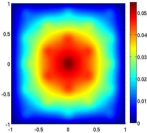
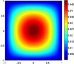
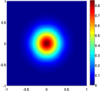
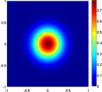
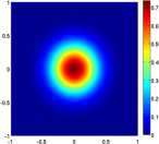
Figure 4: Left and middle columns: Solutions of the heterogenous periodic model (15) for two different values of $\varepsilon$ – pressure $p^{\varepsilon}$ (top) and cell density $C^{\varepsilon}$ (bottom) at time $t=0.05$. In the left column $\varepsilon=0.4$ and in the middle column $\varepsilon=0.05$. Right column: Solution of the homogenized model (32) – pressure $p^{0}$ (top) and cell density $C^{0}$ (bottom) at time $t=0.05$.

Finally we have compared the computational time required to obtain the numerical approximation of the periodic multiscale problem (15) and of the homogenization problem (32). The former takes approximately 1800 seconds to execute a single iteration in time (to obtain $(C^{\varepsilon},p^{\varepsilon})$) with a spatial step size $5e-03$ in $\Omega$, and this is more than seven times larger than the time spent by the homogenized problem, that needs in fact just 250 seconds to obtain $(C^{0},p^{0})$. The main reason for this computational time difference, between the two problems, is due to the fact that the coefficients of the homogenized problem (32) are constants with respect to the spatial variable, whereas this is not the case for coefficients of the periodic multiscale problem (15), and then the latter problem needs a larger time cost.

8 Conclusions

In this paper we derived an homogenization model, for simulating the ACF spread and dynamics, with the goal of reproducing in silico at a macroscopic level (i.e. at the tissue level) what is observed in conventional colonoscopy images. We have considered the PDEs model (15) for the mathematical description of the biological phenomenon. It is an heterogenous periodic model based on the assumption that the colon is a domain, with a periodic distribution of very small heterogeneities, the crypts, wherein most cellular activity occurs. In this model we suppose the existence of an abnormal cell population that has the property to proliferate not only inside the crypts, as done by normal cells, but also outside the crypts. This property is believed to be responsible for abnormal cells to invade neighbor crypts and possibly induce crypt fission and the formation of an adenoma. Then we have applied an homogenization technique to the heterogenous periodic model that relies on the two-scale asymptotic expansion method.

In a previous work [23] we solved numerically an heterogeneous periodic problem, similar to (15), without any homogenization technique, but applying a multi-scale numerical approach. In [23] we have observed that choosing a small size for the heterogeneousness (i.e. the crypt size $\varepsilon$) results in a high cost of memory and computations.

The main benefit of the homogenization model herein proposed, in comparison with the approach developed in [23], is that it permits to describe with a simpler model (the homogenized one) a very complex, periodic and multi-scale problem. For the homogenization model, a numerical solution can be easily computed, by means of standard discretization methods, as finite elements for the spatial variable combined with finite differences for the time variable.

In addition the advantage of this homogenization model is the possibility to perform experiments in silico, that represent simulations of the ACF evolution at a macroscopic, or equivalently, tissue level, starting with an arbitrary density (small or big) of abnormal cells that can be located in an arbitrary colon region (inside a single crypt or in several crypts, adjacent or not, or outside the crypts). In effect, the location and density of the abnormal cells at the initial time is controlled (meaning represented) by the definition of the initial cell density.

In the future we intend to build a more complete hybrid model, by incorporating other biological effects of the ACF formation, such as the crypt fission and the viscoelastic properties of the colon epithelium. This will permit to compare the predicted ACF dynamics with that obtained by medical images and histopathological results.

References

• [1] K. Araki, Y. Furuya, M. Kobayashi, K. Matsuura, T. Ogata, and H. Isozaki. Comparison of microvascularture between the proximal and distal human colon. J. Electron. Microsc., 45:202–206, 1996.
• [2] N. J. Armstrong, K. J. Painter, and J. A. Sherratt. A continuum approach to modelling cell–cell adhesion. Journal of Theoretical Biology, 243:98–113, 2006.
• [3] A. M. Baker et al. Quantification of crypt and stem cell evolution in the normal and neoplastic human colon. Cell Reports, 8:940–947, 2014.
• [4] R. E. Baker, E. A. Gaffney, and P. K. Maini. Partial differential equations for self-organization in cellular and developmental biology. Nonlinearity, 21(11):R251–R290, 2008.
• [5] N.S. Bakhvalov and G. P. Panasenko. Homogenisation: averaging processes in periodic media: mathematical problems in the mechanics of composite materials. Kluwer Academic Publishers, 1989.
• [6] A. Bensoussan, J.L. Lions, and G. Papanicolaou. Asymptotic Analysis for Periodic Structures. North-Holland, Amsterdam, 1978.
• [7] M. Bienz and H. Clevers. Linking colorectal cancer to Wnt signaling. Cell, 103:311–320, 2000.
• [8] R. P. Bird. Role of aberrant crypt foci in understanding the pathogenesis of colon cancer. Cancer Letters, 93:55–71, 1995.
• [9] R. P. Bird and C. K. Good. The significance of aberrant crypt foci in understanding the pathogenesis of colon cancer. Toxicology Letters, 112-113:395–402, 2000.
• [10] B. Boman, J. Fields, K. Cavanaugh, A. Guetter, and O. Runquist. How dysregulated colonic crypt dynamics cause stem cell overpopulation and initiate colon cancer. Cancer Research, 68(9):3304–3313, 2008.
• [11] A. J. Carulli, L. C. Samuelson, and S. Schnell. Unraveling intestinal stem cell behavior with models of crypt dynamics. Integrative Biology, 6(3):243–257, 2014.
• [12] D. Cioranescu and P. Donato. An introduction to homogenization, volume 26. Oxford University Press Oxford, 1999.
• [13] J. Costa, I. Gonzalez-Garcia, and R. Sole. Spatial dynamics in cancer. In Complex Systems Science in Biomedicine, Chapter 6.2, pages 557–577. (Deisboeck, T.S., and Kresh, J.Y.), 2006.
• [14] V. Cristini, X. Li, J. Lowengrub, and S. M. Wise. Nonlinear simulations of solid tumor growth using a mixture model: invasion and branching. Journal of Mathematical Biology, 58:723–763, 2009.
• [15] V. Cristini, J. Lowengrub, and Q. Nie. Nonlinear simulation of tumor growth. Journal of Mathematical Biology, 46:191–224, 2003.
• [16] D. Drasdo and M. Loeffer. Individual-based models to growth and folding in one-layered tissues: intestinal crypts and early development. Nonlinear Analysis, 47:245–256, 2001.
• [17] C. M. Edwards and S.J. Chapman. Biomechanical modelling of colorectal crypt budding and fission. Bulletin of Mathematical Biology, 69(6):1927–1942, 2007.
• [18] B. Engquist and P.E. Souganidis. Asymptotic and numerical homogenization. Acta Numerica, 17:147–190, 2008.
• [19] L. C. Evans. Partial differential equations. Graduate studies in mathematics, volume 19. 1998.
• [20] I. N. Figueiredo and C. Leal. Physiologic parameter estimation using inverse problems. SIAM Journal on Applied Mathematics, 73(3):1164–1182, 2013.
• [21] I. N. Figueiredo, C. Leal, T. Leonori, G. Romanazzi, P. N. Figueiredo, and M.M. Donato. A coupled convection-diffusion level set model for tracking epithelial cells in colonic crypts. Procedia Computer Science, 1(1):955–963, 2010.
• [22] I. N. Figueiredo, C. Leal, G. Romanazzi, B. Engquist, and P. N. Figueiredo. A convection-diffusion-shape model for aberrant colonic crypt morphogenesis. Computing and Visualization in Science, 14(4):157–166, 2011.
• [23] I. N. Figueiredo, G. Romanazzi, C. Leal, and B. Engquist. A multiscale model for aberrant crypt foci. Procedia Computer Science, 18:1026–1035, 2013.
• [24] P. Figueiredo and M. Donato. Cyclooxygenase-2 is overexpressed in aberrant crypt foci of smokers. European Journal of Gastroenterology & Hepatology, 22(10):1271, 2010.
• [25] P. Figueiredo, M. Donato, M. Urbano, H. Goulão, H. Gouveia, C. Sofia, M. Leitão, and Diniz Freitas. Aberrant crypt foci: endoscopic assessment and cell kinetics characterization. International Journal of Colorectal Disease, 24(4):441–450, 2009.
• [26] A. Fletcher, C. Breward, and S. Chapman. Mathematical modeling of monoclonal conversion in the colonic crypt. Journal of Theoretical Biology, 300:118–133, 2012.
• [27] A. Friedman. On quasi-linear parabolic equations of the second order. Journal of Mathematics and Mechanics, 7:793–808, 1958.
• [28] A. Friedman. Partial differential equations of parabolic type. Prentice-Hall, Englewood Cliffs, NJ., 1964.
• [29] A. Friedman. Free boundary problems arising in tumor models. Atti Accad. Naz. Lincei Cl. Sci. Fis. Mat. Natur. Rend. Lincei (9) Mat. Appl., 15(3-4):161–168, 2004.
• [30] L. C. Greaves et al. Mitochondrial DNA mutations are established in human colonic stem cells, and mutated clones expand by crypt fission. Proceedings of the National Academy of Sciences of the United States, 103(3):714–719, 2006.
• [31] H. P. Greenspan. On the growth and stability of cell cultures and solid tumors. Journal of Theoretical Biology, 56(2):229?–242, 1976.
• [32] D. V. Guebel and N. V. Torres. A computer model of oxygen dynamics in human colon mucosa: Implications in normal physiology and early tumor development. Journal of theoretical biology, 250(3):389–409, 2008.
• [33] P. R. Halm and S. T. Halm. Secretagogue response of globet cells and columnar cells in human colonic crypts. Am J Physiol Cell Physiol, 278:C212–C233, 2000.
• [34] P. R. Harper and S. K. Jones. Mathematical models for the early detection and treatment of colorectal cancer. Health Care Management Science, 8:101–109, 2005.
• [35] M.A. Hill. (2016) Embryology gastrointestinal tract - colon histology. Retrieved February 29, 2016, from https://embryology.med.unsw.edu.au/embryology/index.php/File:Colon_histology_005.jpg.
• [36] D. Hurlstone et al. Rectal aberrant crypt foci identified using high-magnification-chromoscopic colonoscopy: biomarkers for flat and depressed neoplasia. American Journal of Gastroenterology, pages 1283–1289, 2005.
• [37] W. Isele and H. Meinzer. Applying computer modeling to examine complex dynamics and pattern formation of tissue growth. Computational and Biomedical Research, 31:476–494, 1998.
• [38] M. D. Johnston, C. M. Edwards, W. F. Bodmer, P. K. Maini, and S. J. Chapman. Mathematical modeling of cell population dynamics in the colonic crypt and in colorectal cancer. Proceedings of the National Academy of Sciences of the United States, 104(10):4008–4013, 2007.
• [39] S. K. Kershaw, H. M. Byrne, D. J. Gavaghan, and J. M. Osborne. Colorectal cancer through simulation and experiment. Systems Biology, IET, 7(3):57–73, 2013.
• [40] J. R. King and S. J. Franks. Mathematical analysis of some multi-dimensional tissue-growth models. European Journal of Applied Mathematics, 15:273–295, 2004.
• [41] Wang L. Komarova, N. Initiation of colorectal cancer. Cell Cycle, 3:1558–1565, 2004.
• [42] S. A. Lamprecht and M. Lipkin. Migrating colonic crypt epithelial cells: primary targets for transformation. Carcinogenesis, 23(11):1777–1780, 2002.
• [43] M. Loeffler, A. Birke, D. Winton, and C. Potten. Somatic mutation, monoclonality and stochastic models of stem cell organization in the intestinal crypt. Theor. Biol., 160:471–491, 1993.
• [44] F. Michor, Y. Iwasa, C. Lengauer, and M. A. Nowak. Dynamics of colorectal cancer. Seminars in Cancer Biology, 15:484–494, 2005.
• [45] F. Michor, Y. Iwasa, H. Rajagopalan, C. Lengauer, and M. A. Nowak. Linear model of colon cancer initiation. Cell Cycle, 3:358–362, 2004.
• [46] G. R. Mirams, A. G. Fletcher, P. K. Maini, and H. M. Byrne. A theoretical investigation of the effect of proliferation and adhesion on monoclonal conversion in the colonic crypt. Journal of Theoretical Biology, 312:143–156, 2012.
• [47] P. J. Murray, J. W. A. Kang, G. R. Mirams, S. Y. Shin, H. M. Byrne, P. K. Maini, and K. H. Cho. Modelling spatially regulated $\beta$-catenin dynamics and invasion in intestinal crypts. Biophysical Journal, 99, 2010.
• [48] P. J. Murray, A. Walter, A. G. Fletcher, C. M. Edwards, M. J Tindall, and P. K. Maini. Comparing a discrete and continuum model of the intestinal crypt. Phys. Biol., 8:026011, 2011.
• [49] M. A. Nowak, N. L Komarova, A. Sengupta, P. V. Jallepalli, I-M. Shih, B. Vogelstein, and C. Lengauer. The role of chromosomal instability in tumor initiation. Proceedings of the National Academy of Sciences, 99(25):16226–16231, 2002.
• [50] J. Osborne, A. Walter, S. Kershaw, G. Mirams, A. Fletcher, P. Pathmanathan, D. Gavaghan, O. E. Jensen, P. K. Maini, and H. M. Byrne. A hybrid approach to multi-scale modelling of cancer. Philosophical Transactions of the Royal Society of London A: Mathematical, Physical and Engineering Sciences, 368(1930):5013–5028, 2010.
• [51] K. J. Painter. Continuous models for cell migration in tissues and applications to cell sorting via differential chemotaxis. Bulletin of Mathematical Biology, 71:1117–1147, 2009.
• [52] C. V. Pao. Nonlinear parabolic and elliptic equations. Plenum Press, New York, 1992.
• [53] U. Paulus, M. Loeffler, J. Zeidler, G. Owen, and C.S. Potten. The differentiation and lineage development of goblet cells in the murine small intestinal crypt: experimental and modelling studies. Journal of Cell Science, 106:473–484, 1993.
• [54] S. L. Preston, W.-M. Wong, A. O.-O. Chan, R. Poulsom, R. Jeffery, R.A. Goodlad, N. Mandir, G. Elia, M. Novelli, W.F. Bodmer, I.P. Tomlinson, and N.A. Wright. Bottom-up histogenesis of colorectal adenomas: Origin in the monocryptal adenoma and initial expansion by crypt fission. Cancer Research, 63:3819–3825, 2003.
• [55] B. Ribba, T. Colin, and S. Schnell. A multiscale mathematical model of cancer, and its use in analyzing irradiation therapies. Theoretical Biology and Medical Modelling, (3:7), 2006.
• [56] L. Roncucci, A. Medline, and W. R. Bruce. Classification of aberrant crypt foci and microadenomas in human colon. Cancer Epidemiology, Biomarkers & Prevention, 1:57–60, 1991.
• [57] T. Roose, S. J. Chapman, and P. K. Maini. Mathematical models of avascular tumor growth. SIAM Review, 49(2):179–208, 2007.
• [58] M. H. Ross, G. I. Kaye, and W. Pawlina. Histology: A Text & Atlas. Fourth Edition. Lippincott Williams & Wilkins, 2003.
• [59] E. Sanchez-Palencia. Non-homogeneous Media and Vibration Theory, volume 127. Lecture Notes in Physics, Springer, Berlin, 1980.
• [60] J. A. Sherratt and M. A. Chaplain. A new mathematical model for avascular tumour growth. Journal of Mathematical Biology, 43:291–312, 2001.
• [61] I-M. Shih et al. Top-down morphogenesis of colorectal tumors. Proceedings of the National Academy of Sciences of the United States, 98(5):2640–2645, 2001.
• [62] B. P. Stewart, B. Wild, et al. World Cancer Report. IARC Press, International Agency for Research on Cancer, 2014.
• [63] L. Tartar. The general theory of homogenization. Lecture Notes of the Unione Matematica Italiana, 7, 2009.
• [64] R. W. Taylor et al. Mitochondrial DNA mutations in human colonic crypt stem cells. The Journal of Clinical Investigation, 112(9):1351–1360, 2003.
• [65] I. M. M. van Leeuwen, H. M. Byrne, O. E. Jensen, and J. R. King. Crypt dynamics and colorectal cancer: advances in mathematical modelling. Cell Proliferation, 39:157–181, 2006.
• [66] I. M. M. van Leeuwen, C. M. Edwards, M. Ilyas, and H. M. Byrne. Towards a multiscale model of colorectal cancer. World Journal of Gastroenterology, 13(9):1399–1407, 2007.
• [67] I. M. M. van Leeuwen et al. An integrative computational model for intestinal tissue renewal. Cell Proliferation, 42(5):619–636, 2007.
• [68] A. C. Walter. A Comparison of Continuum and Cell-based Models of Colorectal Cancer. PhD thesis, University of Nottingham, March 2009.
• [69] J. P. Ward and J. R. King. Mathematical modelling of avascular-tumor growth. IMA Journal of Mathematics Applied in Medicine and Biology, 14:39–69, 1997.