Moment based gene set tests

Abstract

Motivation: Permutation-based gene set tests are standard approaches for testing relationships between collections of related genes and an outcome of interest in high throughput expression analyses. Using $M$ random permutations, one can attain $p$-values as small as $1/(M+1)$. When many gene sets are tested, we need smaller $p$-values, hence larger $M$, to achieve significance while accounting for the number of simultaneous tests being made. As a result, the number of permutations to be done rises along with the cost per permutation. To reduce this cost, we seek parametric approximations to the permutation distributions for gene set tests.

Results: We focus on two gene set methods related to sums and sums of squared $t$ statistics. Our approach calculates exact relevant moments of a weighted sum of (squared) test statistics under permutation. We find moment-based gene set enrichment $p$-values that closely approximate the permutation method $p$-values. The computational cost of our algorithm for linear statistics is on the order of doing $|G|$ permutations, where $|G|$ is the number of genes in set $G$. For the quadratic statistics, the cost is on the order of $|G|^{2}$ permutations which is orders of magnitude faster than naive permutation. We applied the permutation approximation method to three public Parkinson’s Disease expression datasets and discovered enriched gene sets not previously discussed. In the analysis of these experiments with our method, we are able to remove the granularity effects of permutation analyses and have a substantial computational speedup with little cost to accuracy.

Availability: Methods available as a Bioconductor package, npGSEA (www.bioconductor.org).

Contact: larson.jessica@gene.com

1 Introduction

In a genome-wide expression study, researchers often compare the level of gene expression in thousands of genes between two treatments groups (e.g., disease, drug, genotype, etc.). Many individual genes may trend toward differential expression, but will often fail to achieve significance. This could happen for a set of genes in a given pathway or system (a gene set). A number of significant and related genes taken together can provide strong evidence of an association between the corresponding gene set and treatment of interest. Gene set methods can improve power by looking for small, coordinated expression changes in a collection of related genes, rather than testing for large shifts in many individual genes.

Additionally, single gene methods often assume that all genes are independent of each other; this is not likely true in real biological systems. With known gene sets of interest, researchers can use existing biological knowledge to drive their analysis of genome-wide expression data, thereby increasing the interpretability of their results.

Mootha et al., (2003) first introduced gene set enrichment analysis (GSEA) and calculated gene set $p$-values based on Kolmogorov-Smirnov statistics. Since then, there have been many methodological proposals for GSEA; no single one is always the best. For example, some tests are better for a large number of weakly associated genes, while others have better power for a small number of strongly associated genes (Newton et al.,, 2007).

One of the most important differences among gene set methods is the definition of the null hypothesis. Tian et al., 2005 and Goeman and Bühlmann, 2007 (among others) introduce two null hypotheses that differentiate the general approaches for gene set methods. The first measures whether a gene set is more strongly related with the outcome of interest than a comparably sized gene set. Methods of this type typically rely on randomizing the gene labels to test what is often called the competitive null hypothesis. This is problematic because genes are inherently correlated (especially those within a set) and permuting them does not give a rigorous test (Goeman and Bühlmann,, 2007).

The second type of approach is used to determine whether the genes within a set associate more strongly with the outcome of interest than they would by chance, had they been independent of the outcome. Methods that test this self-contained null hypothesis usually judge statistical significance by randomizing the phenotype with respect to expression data and assume that gene sets are fixed. While we acknowledge that the competitive hypothesis is often of interest, we focus on methods that test the self-contained hypothesis in this paper.

A popular self-contained GSEA method is the JG-score (Jiang and Gentleman,, 2007), which determines the the level of enrichment based on averaging linear model statistics. Recently, Ackermann and Strimmer, (2009) compared $261$ different gene set tests, and found particularly good performance from a sum of squared single gene regression coefficients. We extend both the sum and the sum of squared linear statistics approaches with a new method in this paper.

All current GSEA methods are based on permutation approaches. The initial GSEA (Mootha et al.,, 2003) and JG-score (Jiang and Gentleman,, 2007) methods both have closed form null distributions for their enrichment statistics, Gaussian and Kolmogorov-Smirnov, respectively; however, even the authors of these methods acknowledge that these distributions do not give the correct $p$-values and suggest the use of permutation. Lehmann and Romano, (2005) give a concise explanation of how permutation inference works. It is common to approximate the permutation distribution by a large Monte Carlo sample (Eden and Yates, 1933; David, 2008).

Permutation tests are simple to program and do not make parametric distributional assumptions. They also can be applied to almost any statistic we might wish to investigate. However, permutation approaches are often computationally expensive, are subject to random inference, and fail to achieve continuous $p$-values. Each of these drawbacks is described in more depth below.

We have developed a new gene set enrichment approach that approximates the permutation distribution of our corresponding test statistics. We find that our method of moments techniques result in almost exactly the same $p$-values as permutation approaches, but in much less computation time. Through our approach, we are able to obtain refined $p$-values and achieve stringent significance thresholds. We applied our approach to three public expression analyses, and found disease-associated gene sets not previously discovered in these studies.

2 Methods

2.1 The data

For definiteness, we present our notation using the language of gene expression experiments. Let $g$, $h$, $r$, and $s$ denote individual genes and $G$ be a set of genes. The cardinality of $G$ is denoted $|G|$, or sometimes $p$. That is the same letter we use for $p$-value, but the usages are distinct enough that there should be no confusion. Our experiment has $n$ subjects. The subjects may represent patients, cell cultures, or tissue samples.

The expression level for gene $g$ in subject $i$ is $X_{gi}$, and $Y_{i}$ is the target variable on subject $i$. $Y_{i}$ is often a treatment, disease, or other phenotype. We center the variables so that

$$\sum_{i=1}^{n}Y_{i}=\sum_{i=1}^{n}X_{gi}=0,\quad\forall g.$$ (1)

The $X_{gi}$ are not necessarily raw expression values, nor are they restricted to microarray values. In addition to the centering (1) they could have been scaled to have a given mean square. The scaling factor for $X_{gi}$ might even depend on the sample variance for some genes $h\neq g$ if we thought that shrinking the variance for gene $j$ towards the others would yield a more stable test statistic (Smyth,, 2005). We might equally use a quantile transformation, replacing the $j^{\prime}$th largest of the raw $X_{gi}$ by $\Phi^{-1}((j-1/2)/n)$ where $\Phi$ is the Gaussian cumulative distribution function. Further preprocessing may be advised to handle outliers in $X$ or $Y$. We do require that the preprocessing of the $X$’s does not depend on the $Y$’s and vice versa.

2.2 Test statistics

Our measure of association for gene $g$ on our treatment of interest is

$$\hat{\beta}_{g}=\frac{1}{n}\sum_{i=1}^{n}X_{gi}Y_{i}.$$ (2)

If both $X_{gi}$ and $Y_{i}$ are centered and standardized to have variance $1$, then $\hat{\beta}_{g}=\hat{\rho}_{g}$, the sample correlation between $Y$ and gene $g$. The usual $t$-statistic for testing a linear relationship between these variables is $t_{g}\equiv\sqrt{n-2}\hat{\rho}_{g}/(1-\hat{\rho}_{g}^{2})^{1/2}$, which is a monotone transformation of $\hat{\rho}_{g}$.

For reasons of power and interpretability, we apply gene set testing methods instead of just testing individual genes. Linear and quadratic test statistics have been found to be the best performers for gene set enrichment analyses; we thus consider two statistics for our approach:

$$\widehat{T}_{G,w} =\sum_{g\in G}w_{g}\hat{\beta}_{g}\quad\text{and}\quad\widehat{C}_{G,w}=\sum_{g\in G}w_{g}\hat{\beta}_{g}^{2}.$$

The statistic $\widehat{T}_{G,w}$ can approximate the JG score of Jiang and Gentleman, (2007). The JG score is $(1/\sqrt{|G|})\sum_{g\in G}t_{g}$. Taking $w_{g}=\sqrt{n-2}/(\mathrm{sd}(X_{g})\mathrm{sd}(Y))$, where $\mathrm{sd}$ denotes a standard deviation, weights genes similarly to the JG score. Although $\widehat{T}_{G,w}$ with these weights sums statistics equivalent to $t$ statistics, it is not exactly equivalent to the sum of those statistics because of the way $\hat{\rho}_{g}$ appears in the denominator of each $t_{g}$.

The statistic $\widehat{C}_{G,w}$ is a weighted sum of squared sample covariances. Ackermann and Strimmer, (2009) conducted an extensive simulation of gene set methods and found good results for quadratic combinations of per gene test statistics.

The letters $T$ and $C$ are mnemonics for the $t$ and $\chi^{2}$ distributions that resemble the permutation distributions of these quantities. The $w_{g}$ are scalar weights. For the quadratic statistics we will suppose that $w_{g}\geqslant 0$. We won’t need that condition to find moments of $C_{G,w}$, but because we will compare $C_{G,w}$ to a $\chi^{2}$ distribution, it is reasonable to avoid negative weights. Non-negative weights are also used to simplify our algorithm.

Although linear and quadratic test statistics are fairly restricted, they do allow a reasonable amount of customization through the weights $w_{g}$, and they are very interpretable compared to more ad hoc statistics.

2.3 Permutation procedure

A permutation of $\{1,2,\dots,n\}$ is a reordering of $\{1,2,\dots,n\}$. There are $n!$ permutations. We call $\pi$ a uniform random permutation of $\{1,2,\dots,n\}$ if it equals each distinct permutation with probability $1/n!$.

In a permutation analysis, we replace $Y_{i}$ by $\widetilde{Y}_{i}$ where $\widetilde{Y}_{i}=Y_{\pi(i)}$ for $i=1,\dots,n$. Then $\widetilde{\beta}_{g}=(1/n)\sum_{i=1}^{n}X_{gi}\widetilde{Y}_{i}$, and when $\widetilde{Y}$ is substituted for $Y$, $\widehat{T}_{G,w}$ becomes $\widetilde{T}_{G,w}$ and $\widehat{C}_{G,w}$ becomes $\widetilde{C}_{G,w}$.

The $n!$ different permutations form a reference distribution from which we can compute $p$-values. There are often so many possible permutations that we cannot calculate or use all of them. Instead, we independently sample uniform random permutations $M$ times, getting statistics $\widetilde{C}_{m}=\widetilde{C}_{G,w,m}$, and similarly $\widetilde{T}_{m}$, for $m=1,\dots,M$. We then compute $p$-values by comparing our observed statistics to our permutation distribution:

$$p_{Q} =\frac{\#\{\widetilde{C}_{m}\geqslant\widehat{C}\}+1}{M+1} p_{C} =\frac{\#\{|\widetilde{T}_{m}|\geqslant|\widehat{T}|\}+1}{M+1}$$

$$p_{L} =\frac{\#\{\widetilde{T}_{m}\leqslant\widehat{T}\}+1}{M+1},\quad\text{or} p_{R} =\frac{\#\{\widetilde{T}_{m}\geqslant\widehat{T}\}+1}{M+1},$$

where $p_{Q}$ and $p_{C}$ are $p$-values for two-sided inferences on the quadratic and linear statistic, respectively, and $p_{L}$ (left) and $p_{R}$ (right) are for one-sided inferences based on the linear statistic. We use the mnemonic $C$ in $p_{C}$ to denote the central (or two-sided) $p$-value, which corresponds to a central confidence interval. The $+1$ in numerator and denominator of the $p$-values corresponds to counting the sample test statistic as one of the permutations. That is, we automatically include an identity permutation.

2.4 Permutation disadvantages

There are three main disadvantages to permutation-based analyses: cost, randomness, and granularity.

Testing many sets of genes becomes computationally expensive for two reasons. First, there are many test statistics to calculate in each permuted version of the data. Second, to allow for multiplicity adjustment, we require small nominal $p$-values to draw inference about our sets, which in turn requires a large number of permutations. That is, to obtain a small adjusted $p$-value (e.g., via FDR, FWER, Bonferroni methods), one first needs a small enough raw $p$-value. In order to obtain small raw $p$-values, the number of permutations ($M$) must be large, thereby increasing computational cost.

Because permutations are based on a random shuffling of the data, there is a chance that we will obtain a different $p$-value for our set of interest each time we run our permutation analysis. That is, our inference is subject to a given random seed.

Permutations also have a granularity problem. If we do $M$ permutations, then the smallest possible $p$-value we can attain is $1/(M+1)$. At or below this minimum $p$-value permutation tests have no power. Knijnenburg et al., (2009) suggest that for a reliable $p$-value, there should be at least $10$ permuted values more extreme than the sample. That requires $M\approx 10/p$ and when it is necessary, due to test multiplicity, to use small $p$ such as $10^{-6}$ or smaller, the permutation approach becomes computationally expensive. We call this the sample granularity problem.

There is also a population granularity problem. In an experiment with $n$ observations, the smallest possible $p$-value is at least $1/n!$. Sometimes the attainable minimum is much larger. For instance, when the target variable $Y$ is binary with $n/2$ positive and $n/2$ negative values then the smallest possible $p$-value is $1/{n\choose n/2}$. For $n=10$ we necessarily have $p\geqslant 1/252$. Rotation sampling methods such as ROAST are able to get around this population granularity problem (Wu et al.,, 2010). Increased Monte Carlo sampling can mitigate the sample granularity problem but not the population granularity problem.

Another aspect of the granularity problem is that permutations give us no basis to distinguish between two gene sets that both have the same $p$-value $1/(M+1)$. There may be many such gene sets, and they have meaningfully different effect sizes. Many current approaches solve this problem by ranking significantly enriched gene sets by their corresponding test statistics. This practice only works if all test statistics have the same null distribution and correlation structure, which is not the case for many current GSEA methods. Additionally, the resulting broken ties do not have a $p$-value interpretation and cannot be directly used in multiple testing methods. To break ties in this way also requires the retention of both a $p$-value and a test statistic for inference, rather than just one value.

Because of each of these limitations of permutation testing, there is a need to move beyond permutation-based GSEA methods. The methods we present below are not as computationally expensive, random, or granular as their permutation counterparts. Our proposal results in a single number on the $p$-value scale.

2.5 Moment based reference distributions

To avoid the issues discussed above, we approximate the distribution of the permuted test statistics $\widetilde{T}_{G,w}$ by Gaussians or by rescaled beta distributions. For quadratic statistics $\widetilde{C}_{G,w}$ we use a distribution of the form $\sigma^{2}\chi^{2}_{(\nu)}$ choosing $\sigma^{2}$ and $\nu$ to match the second and fourth moments of $\widetilde{C}_{G,w}$ under permutation.

For the Gaussian treatment of $\widetilde{T}_{G,w}$ we find $\sigma^{2}=\mathrm{var}(\widetilde{T}_{G,w})$ under permutation using equation (5) of Section 3.3 and then report the $p$-value

$$p=\Pr(\mathcal{N}(0,\sigma^{2})\leqslant\widehat{T}_{G,w}),$$

where $\widehat{T}_{G,w}$ is the observed value of the linear statistic. The above is a left tail $p$-value. Two-tailed and right-tailed $p$ values are analogous.

When we want something sharper than the normal distribution, we can use a scaled Beta distribution, of the form $A+(B-A)\mathrm{beta}(\alpha,\beta)$. The $\mathrm{beta}(\alpha,\beta)$ distribution has a continuous density function on $0<x<1$ for $\alpha,\beta>0$. We choose $A$, $B$, $\alpha$ and $\beta$ by matching the upper and lower limits of $\widetilde{T}_{G,w}$, as well as its mean and variance. Using equation (5) from our theory section we have

$$\begin{split}A&=\min_{\pi}\frac{1}{n}\sum_{i=1}^{n}\sum_{g\in G}w_{g}X_{gi}Y_{\pi(i)},\\ B&=\max_{\pi}\frac{1}{n}\sum_{i=1}^{n}\sum_{g\in G}w_{g}X_{gi}Y_{\pi(i)},\\ \alpha&=\frac{A}{B-A}\Bigl{(}\frac{AB}{\mathrm{var}(\widetilde{T}_{G,w})}+1\Bigr{)},\quad\text{and}\\ \beta&=\frac{-B}{B-A}\Bigl{(}\frac{AB}{\mathrm{var}(\widetilde{T}_{G,w})}+1\Bigr{)}.\end{split}$$ (3)

The observed left-tailed $p$-value is

$$p=\Pr\Bigl{(}\mathrm{beta}(\alpha,\beta)\leqslant\frac{\widehat{T}_{G,w}-A}{B-A}\Bigr{)}.$$

It is easy to find the permutations that maximize and minimize $\widetilde{T}_{G,w}$ by sorting the $X$ and $Y$ values appropriately as described in Section 3.3. The result has $A<0<B$. For the beta distribution to have valid parameters we must have $\sigma^{2}<-AB$. From the inequality of Bhatia and Davis, (2000), we know that $\sigma^{2}\leqslant-AB$. There are in fact degenerate cases with $\sigma^{2}=-AB$, but in these cases $\widetilde{T}_{G,w}$ only takes one or two distinct values under permutation, and those cases are not of practical interest.

Like us, Zhou et al. (2009) have used a beta distribution to approximate a permutation. They used the first 4 moments of a Pearson curve for their approach. Fitting by moments in the Pearson family, it is possible to get a beta distribution whose support set $(A,B)$ does not even include the observed value. That is, the observed value is even more extreme than it would have to be to get $p=0$; it is almost like getting $p<0$. We chose $(A,B)$ based on the upper and lower limits of $\widetilde{T}_{G,w}$ to prevent our observed test statistic from falling outside the range of possible values of our reference distribution (Section 3.3).

For the quadratic test statistic $\widehat{C}_{G,w}$ we use a $\sigma^{2}\chi^{2}_{(\nu)}$ reference distribution reporting the two-tailed $p$-value $\Pr(\sigma^{2}\chi^{2}_{(\nu)}\geqslant\widehat{C}_{G,w})$ after matching the first and second moments of $\sigma^{2}\chi^{2}_{(\nu)}$ to $\mathbb{E}(\widetilde{C}_{G,w})$ and $\mathbb{E}(\widetilde{C}_{G,w}^{2})$ respectively. The parameter values are

$$\nu=2\frac{\mathbb{E}(\widetilde{C}_{G,w})^{2}}{\mathrm{var}(\widetilde{C}_{G,w})}\quad\text{and}\quad\sigma^{2}=\frac{\mathbb{E}(\widetilde{C}_{G,w})}{\nu}=\frac{\mathrm{var}(\widetilde{C}_{G,w})}{2\mathbb{E}(\widetilde{C}_{G,w})}.$$

Our formulas for $\mathbb{E}(\widetilde{C}_{G,w})$ and $\mathbb{E}(\widetilde{C}_{G,w}^{2})$ under permutation are given in equation (4) of Section 3.1. Those formulas use $\mathbb{E}(\widetilde{\beta}_{g}^{2})$ and $\mathrm{cov}(\widetilde{\beta}_{g}^{2},\widetilde{\beta}_{h}^{2})$ which we give in Corollaries 1 and 2 of Section 3.1.

All of our reference distributions are continuous and unbounded and hence they avoid the granularity problem of permutation testing. We have prepared a publicly available Bioconductor (Gentleman et al.,, 2004) package, npGSEA, which implements our algorithm and calculates the corresponding statistics discussed in this section.

3 Theoretical results

3.1 Permutation moments of test statistics

Under permutation, $\mathbb{E}(\widetilde{Y}_{i})=0$ by symmetry, and so $\mathbb{E}(\widetilde{\beta}_{g})=0$ too. We easily find that,

$$\begin{split}\mathbb{E}(\widetilde{T}_{G,w})&=0,\\ \mathrm{var}(\widetilde{T}_{G,w})&=\sum_{g\in G}\sum_{h\in G}w_{g}w_{h}\mathrm{cov}(\widetilde{\beta}_{g},\widetilde{\beta}_{h})\\ \mathbb{E}(\widetilde{C}_{G,w})&=\sum_{g\in G}w_{g}\mathbb{E}(\widetilde{\beta}_{g}^{2}),\quad\text{and}\\ \mathrm{var}(\widetilde{C}_{G,w})&=\sum_{g\in G}\sum_{h\in G}w_{g}w_{h}\mathrm{cov}(\widetilde{\beta}^{2}_{g},\widetilde{\beta}^{2}_{h}).\end{split}$$ (4)

The means, variances and covariances in (4) are taken with respect to the random permutations with the data $X$ and $Y$ held fixed. We adopt the convention that moments of permuted quantities are taken with respect to the permutation and are conditional on the $X$’s and $Y$’s. This avoids cumbersome expressions like $\mathbb{E}(\widetilde{\beta}^{2}_{g}\mid X_{gi},Y_{i},g\in G)$.

We will need the following even moments of $X$ and $Y$:

$$\mu_{2} =\frac{1}{n}\sum_{i=1}^{n}Y_{i}^{2},\quad\mu_{4}=\frac{1}{n}\sum_{i=1}^{n}Y_{i}^{4},$$

$$\bar{X}_{gh} =\frac{1}{n}\sum_{i=1}^{n}X_{gi}X_{hi},\quad\text{and}$$

$$\bar{X}_{ghrs} =\frac{1}{n}\sum_{i=1}^{n}X_{gi}X_{hi}X_{ri}X_{si}$$

for $g,h,r,s\in G$. Although our derivations involve $O(p^{4})$ different moments when the gene set $G$ has $p$ genes, our computations do not require all of those moments.

Lemma 1.

For an experiment with $n\geqslant 2$ including genes $g$ and $h$,

$$\mathbb{E}(\widetilde{\beta}_{g}\widetilde{\beta}_{h})=\frac{\mu_{2}\bar{X}_{gh}}{n-1}.$$

Proof.

See Appendix 1. $\Box$ ∎

Corollary 1.

For an experiment with $n\geqslant 2$ including genes $g$ and $h$,

$$\mathrm{cov}(\widetilde{\beta}_{g},\widetilde{\beta}_{h})=\mu_{2}\bar{X}_{gh}/(n-1).$$

Proof.

This follows from Lemma 1 because $\mathbb{E}(\widetilde{\beta}_{g})=0$. ∎

From Corollary 1, we see that the correlation between permuted test statistics $\widetilde{\beta}_{g}$ and $\widetilde{\beta}_{h}$ is simply the correlation between expression values for genes $g$ and $h$.

Lemma 2.

For an experiment with $n\geqslant 4$ including genes $g,h,r,s$,

$$\mathbb{E}(\widetilde{\beta}_{g}\widetilde{\beta}_{h}\widetilde{\beta}_{r}\widetilde{\beta}_{s})=\begin{pmatrix}\mu_{2}^{2}\\ \mu_{4}\end{pmatrix}^{\mathsf{T}}A^{\mathsf{T}}B\begin{pmatrix}\bar{X}^{*}_{ghrs}/n^{2}\\[4.30554pt] \bar{X}_{ghrs}/n^{3}\end{pmatrix}$$

where $\bar{X}^{*}_{ghrs}=\bar{X}_{gh}\bar{X}_{rs}+\bar{X}_{gs}\bar{X}_{hr}+\bar{X}_{gr}\bar{X}_{hs}$, with $A^{\mathsf{T}}$ given by

$$\begin{pmatrix}0&0&\dfrac{n}{n-1}&\dfrac{-n}{(n-1)(n-2)}&\dfrac{3n}{(n-1)(n-2)(n-3)}\\[8.61108pt] 1&\dfrac{-1}{n-1}&\dfrac{-1}{n-1}&\dfrac{2}{(n-1)(n-2)}&\dfrac{-6}{(n-1)(n-2)(n-3)}\end{pmatrix},$$

and

$$B =\begin{pmatrix}\phantom{-}0&\phantom{-}1\\ \phantom{-}0&-4\\ \phantom{-}1&-3\\ -2&\,12\\ \phantom{-}1&-6\end{pmatrix}.$$

Proof.

See Appendix 2. $\Box$ ∎

The expression is complicated, but it is simple to compute; we need only two moments of $Y$, two cross-moments of $X$, and the $2\times 2$ matrix $A^{\mathsf{T}}B$. The matrix $A$ depends on the experiment through $n$. Using Lemma 2 we can obtain the covariance between $\widetilde{\beta}^{2}_{g}$ and $\widetilde{\beta}^{2}_{h}$.

Corollary 2.

For an experiment with $n\geqslant 4$ and genes $g,h$,

$$\mathrm{cov}(\widetilde{\beta}^{2}_{g},\widetilde{\beta}^{2}_{h}) =\begin{pmatrix}\mu_{2}^{2}\\ \mu_{4}\end{pmatrix}^{\mathsf{T}}A^{\mathsf{T}}B\begin{pmatrix}\bar{X}^{*}_{gghh}/n^{2}\\[4.30554pt] \bar{X}_{gghh}/n^{3}\end{pmatrix}-\frac{\mu_{2}^{2}}{(n-1)^{2}}\bar{X}_{gg}\bar{X}_{hh},$$

where $\bar{X}^{*}_{gghh}=\bar{X}_{gg}\bar{X}_{hh}+2\bar{X}_{gh}^{2}$ with $A$ and $B$ as given in Lemma 2.

Proof.

The covariance is $\mathbb{E}(\widetilde{\beta}^{2}_{g}\widetilde{\beta}^{2}_{h})-\mathbb{E}(\widetilde{\beta}^{2}_{g})\mathbb{E}(\widetilde{\beta}^{2}_{h})$. Applying Lemma 2 to the first expectation and Lemma 1 to the other two yields the result.  $\Box$ ∎

3.2 Rotation moments of test statistics

Rotation sampling (Wedderburn,, 1975; Langsrud,, 2005) provides an alternative to permutations, and is justified if either $X$ or $Y$ has a Gaussian distribution. It is simplest to describe when $Y\sim\mathcal{N}(\mu,\sigma^{2}I_{n})$ and even simpler for $Y\sim\mathcal{N}(0,\sigma^{2}I_{n})$. In the latter case we can replace $Y$ by $\widetilde{Y}=QY$ where $Q\in\mathbb{R}^{n\times n}$ is a random orthogonal matrix (independent of both $X$ and $Y$), and the distribution of our test statistics is unchanged under the null hypothesis that $X$ and $Y$ are independent.

Rotation tests work by repeatedly sampling from the uniform distribution on random orthogonal matrices and recomputing the test statistics using $\widetilde{Y}$ instead of $Y$. They suffer from sample granularity but not population granularity because $Q$ has a continuous distribution (for $n\geqslant 2$).

To take account of centering we need to use a rotation test appropriate for $Y\sim\mathcal{N}(\mu,\sigma^{2}I_{n})$. Langsrud, (2005) does this by choosing rotation matrices that leave the population mean fixed. He rotates the data in an $n-1$ dimensional space orthogonal to the vector $1_{n}$. To get such a rotation matrix, he first selects an orthogonal contrast matrix $W\in\mathbb{R}^{n\times(n-1)}$. This matrix satisfies $W^{\mathsf{T}}W=I_{n-1}$ and $W^{\mathsf{T}}1_{n}=0_{n-1}$. Then he generates a uniform random rotation $Q^{*}\in\mathbb{R}^{(n-1)\times(n-1)}$ and delivers $\widetilde{Y}=QY$, where $Q=\frac{1}{n}1_{n}1_{n}^{\mathsf{T}}+WQ^{*}W^{\mathsf{T}}$. More generally if $Y\sim\mathcal{N}(Z\gamma,\sigma^{2}I_{n})$, for a linear model $Z\gamma$, Langsrud, (2005) shows how to rotate $Y$ in the residual space of this model, leaving the fits unchanged.

Wu et al., (2010) have implemented rotation sampling for microarray experiments in their method, ROAST. They speed up the sampling by generating a random vector instead of a random matrix. For some tests, permutations and rotations have the same moments, and so our approximations are approximations of rotation tests as much as of permutation tests.

Our rotation method approximation performs very similarly to the permutation method. We let $\widetilde{Y}=QY$ for $Q=(\frac{1}{n}1_{n}1_{n}^{\mathsf{T}}+WQ^{*}W^{\mathsf{T}})$ where $Q^{*}$ is a uniform random $n-1\times n-1$ rotation matrix and the contrast matrix $W\in\mathbb{R}^{n\times(n-1)}$ satisfies $W^{\mathsf{T}}1_{n}=0_{n-1}$ and $W^{\mathsf{T}}W=I_{n-1}$ and then $\widetilde{\beta}$, $\widetilde{T}$ and $\widetilde{C}$ are defined as for permutations, substituting $\widetilde{Y}$ for $Y$.

The variance of the quadratic test statistic depends on which contrast matrix $W$ one chooses, and it cannot always match the permutation variance. This difference disappears asymptotically as $n\to\infty$.

Lemma 3.

For an experiment with $n\geqslant 2$ including genes $g$ and $h$, the moments $\mathbb{E}(\widetilde{\beta}_{g})$ and $\mathbb{E}(\widetilde{\beta}_{g}\widetilde{\beta}_{h})$ are identical to their permutation counterparts, regardless of the choice for $W$.

Proof.

See Appendix 3 and 4. $\Box$ ∎

Corollary 3.

For an experiment with $n\geqslant 2$, $\mathbb{E}(\widetilde{T}_{G,w})$, $\mathrm{var}(\widetilde{T}_{G,w})$ and $\mathbb{E}(\widetilde{C}_{G,w})$ are the same whether $\widetilde{Y}$ is formed by permutation or rotation of $Y$.

3.3 Computation and costs

To facilitate computation for the linear statistic, we reduce each gene set to a single pseudo-gene $X_{Gi}=\sum_{g\in G}w_{g}X_{gi}$ and then let

$$\bar{X}_{G}=\frac{1}{n}\sum_{i=1}^{n}X_{Gi}\quad\text{and}\quad\bar{X}_{GG}=\frac{1}{n}\sum_{i=1}^{n}X_{Gi}^{2}.$$

The weights $w$ have been absorbed into the pseudo-gene to simplify notation. We define

$$\hat{\beta}_{G} =\sum_{g\in G}w_{g}\hat{\beta}_{g}=\frac{1}{n}\sum_{i}X_{Gi}Y_{i},\quad\text{and}$$

$$\widetilde{\beta}_{G} =\sum_{g\in G}w_{g}\widetilde{\beta}_{g}=\frac{1}{n}\sum_{i}X_{Gi}\widetilde{Y}_{i}.$$

Our permuted linear test statistic is $\widetilde{T}_{G,w}=\widetilde{\beta}_{G}$, with

$$\mathrm{var}(\widetilde{T}_{G,w}) =\mathrm{var}(\widetilde{\beta}_{G})=\frac{\mu_{2}}{n-1}\bar{X}_{GG}.$$ (5)

For the beta approximation, we need the range of $\widetilde{T}_{G,w}$. Let the sorted $Y$ values be $Y_{(1)}\leqslant Y_{(2)}\leqslant\dots\leqslant Y_{(n)}$ and the sorted $X_{Gi}$ values be $X_{G(1)}\leqslant X_{G(2)}\leqslant\dots\leqslant X_{G(n)}$. Then the range of $\widetilde{T}_{G,w}$ is $[A,B]$, where

$$A =\frac{1}{n}\sum_{i=1}^{n}X_{G(i)}Y_{(n+1-i)},\quad\text{and}\quad B=\frac{1}{n}\sum_{i=1}^{n}X_{G(i)}Y_{(i)}.$$

For a $\sigma t_{(\nu)}$ reference distribution we would also need $\mathbb{E}(\widetilde{T}_{G,w}^{4})=\mathbb{E}(\widetilde{\beta}_{G}^{4})$. We can apply Lemma 2 to the pseudo-gene resulting in

$$\mathbb{E}(\widetilde{\beta}_{G}^{4})=\begin{pmatrix}\mu_{2}^{2}\\ \mu_{4}\end{pmatrix}A^{\mathsf{T}}B\begin{pmatrix}3\bar{X}_{GG}^{2}/n^{2}\\ \bar{X}_{GGGG}/n^{3}\end{pmatrix},$$ (6)

where $\bar{X}_{GGGG}=\frac{1}{n}\sum_{i=1}^{n}X_{Gi}^{4}$.

We considered using a $\sigma t_{(\nu)}$ reference distribution for $\widetilde{T}_{G,w}$, taking into account the fourth moment of $\widetilde{T}_{G,w}$  (6). We have often (in fact usually) found that $\mathbb{E}(\widetilde{T}_{G,w}^{4})<3\mathbb{E}(\widetilde{T}_{G,w}^{2})^{2}$; that is, lighter tails than the normal. This implies a negative kurtosis for the permutation distribution, and $t$ distributions have positive kurtosis. For this reason we use a beta approximation and not a $t$ approximation.

For the quadratic statistic we have found it useful to replace $X_{gi}$ by $\sqrt{w_{g}}X_{gi}$ in precomputation. That step is only valid for non-negative $w_{g}$, but those are the ones of most interest. Then we use formulas for $\mathbb{E}(\widetilde{C}_{G,w})$ and $\mathrm{var}(\widetilde{C}_{G,w})$ with all $w_{g}=w_{h}=1$  (4).

Now we consider the computational cost. The cost to compute all of the $X_{Gi}$ is dominated by $np$ multiplications. It then takes $n$ more multiplications to get $\hat{\beta}_{G}$ and another $n$ to get $\bar{X}_{GGe}$. It costs $n$ multiplications to get all the $\mu_{2}$, except that step done once can be used for all gene sets. The cost for the Gaussian approximation $\mathcal{N}(0,\mathrm{var}(\widetilde{T}_{G,w}))$ is dominated by $n(p+2)$ multiplications.

For the beta approximation there is also a cost proportional to $n\log(n)$ in the sorting to compute limits $A$ and $B$. That adds a cost comparable to a multiple of $\log(n)$ permutations. We judge that the cost of sorting is usually minor for $n$ and $p$ of interest in bioinformatics.

A permutation analysis requires $nM$ multiplications, after computing $X_{Gi}$, for a total of $n(M+p)$. It is very common for $p$ to be a few tens and $M$ to be many thousands or more. Then we can simplify the costs to $n(M+p)\approx nM$ and $n(2+p)\approx np$. The moment method costs about as much as doing $p$ permutations. When the gene set has tens of genes and the permutation method uses many thousands or even several million permutations, the computational cost is quite large.

The pseudo-gene technique is more expensive for the quadratic statistics. The dominant cost in computing $\widehat{C}_{G,w}$ is still the $np$ multiplications required to compute $\widehat{\beta}_{g}$ for $g\in G$. We can also compute $\mathbb{E}(\widetilde{C}_{G,w})$ in about this amount of work.

The cost of computing $\mathrm{var}(\widetilde{C}_{G,w})$ by a straightforward algorithm is at least $np^{2}$, because we need $\bar{X}_{gh}$ and $\bar{X}_{gghh}$ for all $g,h\in G$. Some parts of that computation can be sped up to $O(np)$ by rewriting the expression as described in Appendix 5. One of the terms however does not reduce to $O(np)$. A straightforward implementation costs $O(np^{2})$ while an alternative expression costs $O(n^{2}p)$. The latter is valuable in settings where the gene sets are large compared to the sample size. In the former case, the moment approximation has cost comparable to $O(p^{2})$ permutations. If $n<p$ then the latter case is like $np$ permutations, so the quadratic cost is comparable to on the order of $p*\min(n,p)$ permutations.

We have verified our moment formulas by finding that they match values found by enumerating all $n!$ permutations, for some simulated data sets with small $n$. During testing, we also compared permutation and our approximate $p$-values on simulated data. We saw a close match but think that an illustration on real data is more compelling. Section 4 makes comparisons using three genome wide expression studies in Parkinson’s Disease (PD) patients: Moran et al., (2006), Scherzer et al., (2007) and Zhang et al., (2005).

4 Parkinson’s Disease

We illustrate our method using publicly available data from three expression studies in Parkinson’s Disease (PD) patients (Moran et al., 2006, Zhang et al., 2005, and Scherzer et al., 2007; Table 1). All three experiments contain genome wide expression values measured via a microarray experiment. PD is a common neurodegenerative disease; clinical symptoms often include rigidity, resting tremor and gait instability (Abou-Sleiman et al.,, 2006). Pathologically, PD is characterized by neuronal-loss in the substantia nigra and the presence of $\alpha$-synuclein protein aggregates in neurons (Abou-Sleiman et al.,, 2006).

Reference	Tissue	# Affected	# Controls
Moran	Substantia nigra	29	14
Zhang	Substantia nigra	18	11
Scherzer	Blood	47	21

Table 1: Three data sets used for non-permutation GSEA

Using a selected set from the Broad Institute’s mSigDB v3.1 (Subramanian et al.,, 2005) and the presence of PD as a response variable from the Zhang et al., (2005) dataset, we visualized both permutation distributions and our approximation of these distributions (Figure 1). As discussed above, we use a linear test statistic, $\widehat{T}_{G,w}=\sum_{g\in G}\hat{\beta}_{g}$, and a quadratic test statistic, $\widehat{C}_{G,w}=\sum_{g\in G}\hat{\beta}_{g}^{2}$, where $\hat{\beta}_{g}$ is a sample covariance between gene expression and, in this case, disease status. Figure 1 shows these two test statistics with a histogram of $99{,}999$ recomputations of those statistics for permutations of treatment status versus gene expression. In principle, histograms of permuted test statistics can be very complicated, but in practice, they often resemble familiar parametric distributions, as in Figure 1.

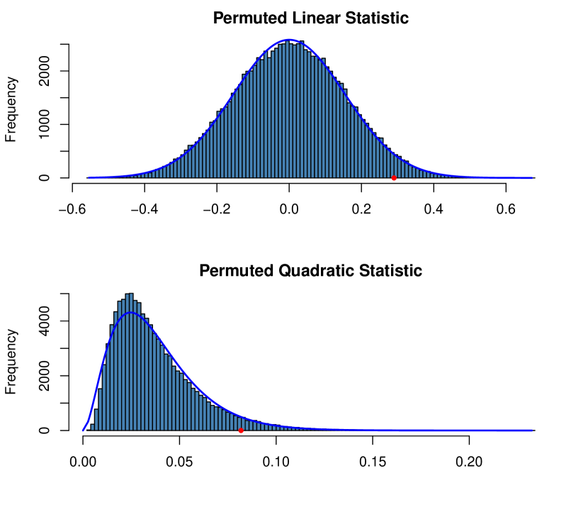
Figure 1: Top panel shows a permutation histogram for a linear test statistic for the the steroid hormone signaling pathway gene set as described in the text. The bottom panel shows a quadratic test statistic. Solid red dots indicate the observed values and curves indicate parametric fits, based on normal and $\chi^{2}$ distributions.

Using the fitted normal distribution to determine the rarity of the observed gene set statistic results in a two-tailed $p$-value of $0.0604$ for the linear statistic while permutations yield $p=0.0595$. A fitted $\sigma^{2}\chi^{2}_{(\nu)}$ distribution results in $p=0.0425$ for the sum of squares gene set statistic, while permutations yield $p=0.0458$. The $p$-values are a quite close despite the somewhat higher peak for the permutation histogram relative to the $\chi^{2}$ density.

We compared our non-permutation $p$-values to $p$-values for linear and quadratic statistics for the $6{,}303$ gene sets from mSigDB’s curated gene sets and Gene Ontology (GO, Ashburner et al., 2000) gene sets collections (v3.1). One gene set was removed because it contained only one gene in our experiments. The average size of these gene sets is $79.40$ genes. For our gold standard we ran $999{,}999$ permutations of the linear statistic and $499{,}999$ permutations of the quadratic statistic. For all of our permutations, we first calculated the observed test statistic for each of the $6{,}303$ gene sets and then permuted the $Y_{i}$’s $M$ times to obtain $6{,}303$ $\times$ $M$ permuted test statistics. We next compared the pre-computed test statistic vector to our matrix of permuted test statistics.

For each set, we computed left-sided $p$-values, $p_{L}$, for the linear statistic and two-sided $p$-values, $p_{Q}$, for the quadratic statistic using these permutations. We also computed the normal and beta approximations of $p_{L}$ with our method. (Figure 2, left panel). We converted these one-sided $p$-values to two-sided $p$-values via $p=2\min(p_{L},1-p_{L})$. The beta approximation $p$-values are almost identical to the permutation $p$-values.

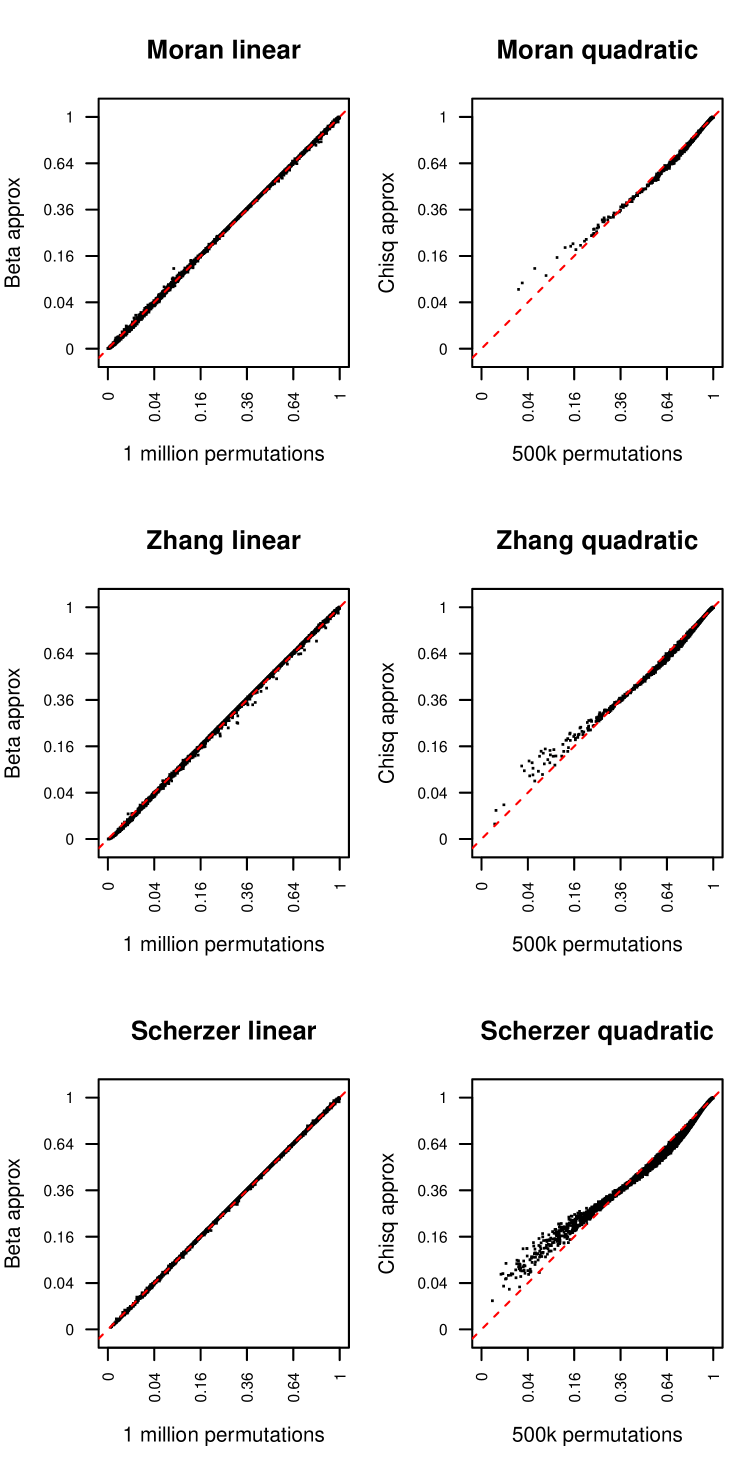
Figure 2: Permutation $p$-values (x-axis) versus moment-based $p$-values (y-axis) for $6{,}303$ gene sets. The left column represents results for a linear test statistic, the right column for sum of squares. Data come from three genome-wide expression studies. We applied the non-linear transformation $p^{1/2}$ to stretch the lower range of these distributions for a more informative visual. Red dotted line represents the line $y=x$.

For our quadratic test statistic, we fit our moment based $\sigma^{2}\chi^{2}_{(\nu)}$ approximation and computed two-sided tailed $p$-values across all sets (Figure 2, right panel). We see that the smallest $\chi^{2}$ non-permutation $p$-values are slightly conservative. This may reflect the boundedness of the permutation distribution combined with the unbounded right tail of the $\chi^{2}$ distribution.

In each of the three experiments, there is a tight correlation between the permutation-based $p$-values of all sets and both of our moment-based methods (Table 2). The beta and normal approximations are almost identical. Our beta approximations are slightly closer to the gold standard than the normal approximations, but not by a practically important amount. The beta approximation has shorter tails than the Gaussian approximation. It yielded $p$-values somewhat smaller than permutations did, while the Gaussian approximation yielded $p$-values somewhat larger than the permutations did. The $\chi^{2}$ approximations also reproduce the ranking of the gold standard quite well, though not as well as the normal and beta approximations to the linear statistic.

Reference	Normal $p_{L}$	Beta $p_{L}$	Normal $p_{C}$	Beta $p_{C}$	Chisq $p_{Q}$
Moran	0.99991	0.99997	0.99973	0.99991	0.978
Zhang	0.99996	0.99997	0.99983	0.99991	0.990
Scherzer	0.99998	0.99999	0.99991	0.99997	0.994

Table 2: Spearman correlations between gold standard ($999{,}999$ and $499{,}999$ permutations for linear and quadratic statistics) and approximation $p$-values. $p_{L}$ and $p_{C}$ represent results for one and two-tailed linear test statistics, respectively. Chisq $p_{Q}$ represents results for the sum of squares analysis.

For these data sets and $6{,}303$ gene sets, both of the linear statistics, which have more or less the same rank-ordering of $p$-values as $999{,}999$ permutations, could be approximated in about than the amount of time it takes to compute $100$ permutations (Table 3, top block). Our gene sets had an average size of about 80 genes. This lead us to expect that the cost of the linear approximation would be comparable to doing 80 permutations. We found that the Gaussian approximation cost about as much as 100 permutations. While this is a close match, we remark that the time to do $M$ permutations is nearly an affine function $a+bM$ with positive intercept $a$. At such small $M$ the overhead costs dominated the total cost making the per permutation costs hard to resolve. The beta approximation was slightly slower than the Gaussian one because it involves the sorting of the data.

Method	Moran	Zhang	Scherzer
$M=100$	31.03	29.84	34.71
$M=500$	31.95	32.49	35.54
$M=1{,}000{,}000$	5010.17	4434.77	3933.15
Normal	29.74	27.00	34.66
Beta	30.79	31.88	37.89
$M=30{,}000$	9146.27	7217.59	11808.02
$M=40{,}000$	12256.54	9636.06	16545.60
$M=50{,}000$	16833.08	12564.06	21480.80
$M=500{,}000$	149588.37	129667.73	187067.91
$\chi^{2}$	11020.62	10600.82	12677.15

Table 3: Time in seconds for $p$-value calculations for $6{,}303$ gene sets in three genome-wide expression studies. Linear statistic results with $M=100$, $M=500$, and $M=1{,}000{,}000$ permutations, and the normal and beta approximations are in the top block. Timings for the quadratic statistic with $M=30{,}000$, $M=40{,}000$, $M=50{,}000$, and $M=500{,}000$ permutations, and the $\chi^{2}$ approximation are presented in the bottom block.

The $\chi^{2}$ approximation to the quadratic statistic has a computational cost about as much as $35{,}000$ to $45{,}000$ permutations, yet has a similar rank-ordering of $p$-values $499{,}999$ permutations (Table 3, bottom block). For the quadratic statistic we expected our algorithm to cost as much as doing a number of permutations equal to a small multiple of the mean square gene set size. It cost about as much as $35{,}000$ to $45{,}000$ permutations while the mean square set size was $27{,}171$.

After applying our permutation approximation methods to each dataset in $6{,}303$ mSigDB gene sets, we found many significantly enriched gene sets, even after correcting for multiple testing (two-sided adjusted $p$-value $<$ 0.05). The most significantly enriched sets are associated with metabolism and mitochondrial function, neuronal transmitters and serotonin, epigenetic modifications, and the transcription factor FOXP3 Supplemental Table 1 Each of these categories has some previously discovered association with PD, although not through traditional gene set methods (metabolism and mitochondrial function: Abou-Sleiman et al., (2006); neuronal transmitters and serotonin: Fox et al., (2009); epigenetic modifications: Berthier and Pulido, (2013); FOXP3: Stone et al., (2009)). Through our new gene set enrichment method, we discovered a relationship between the expression of these gene sets and PD.

5 Discussion

Gene set methods are able to pool weak single gene signals over a set of genes to get a stronger inference. These methods and their corresponding permutation-based inferences are a staple of high throughput methods in genomics. Because an experiment for this purpose may have a few to hundreds of microarrays or RNA-seq samples, permutation can be computationally costly, and yet still result in granular $p$-values. In this paper, we introduce an approximation gene set method, which performs as well as permutation methods, in a fraction of the computation time and which generates continuous $p$-values.

Permutation methods have some valuable properties that our approach does not share. Permutation based inferences give exact $p$-values. Our approximations are not ordinarily exact because the permutation histogram is not in the parametric family we use.

The second advantage of permutations is that they apply to arbitrarily complicated statistics. In our view, many of those complicated statistics are much harder to interpret and are less intuitive than the plain sum and sum of squared statistics we present. Others have observed that simple linear and squared statistics outperform more complex approaches (Ackermann and Strimmer,, 2009). Our method allows for the weighting of coefficients in our statistics, granting users access to additional useful and interpretable patterns.

Because of the disadvantages discussed above, there has long been interest in finding approximations to permutation tests. Eden and Yates, (1933) noticed that the permutation distribution closely matched a parametric distribution that one would get running an $F$-test on the same data. It has also been known since the 1940s that the permutation distribution of the linear test is asymptotically normal as $n$ increases (Good,, 2004). More recently, Knijnenburg et al., (2009) approach the granularity issue by taking a random sample of permutations and fitting a generalized extreme value (GEV) distribution to the tail of their distribution.

Our work differs from these previous permutation approximation approaches. We use Gaussian or beta distributions for the linear statistic and a $\chi^{2}$ distribution for the quadratic statistic. These choices never place the observed test statistic strictly outside the possible range of our reference distribution. In this way, we also avoid nonsensical $p$-values.

We have developed a new and intuitive method for gene set enrichment analysis that is computationally inexpensive, as accurate as permutation methods, and avoids the sample granularity issue. A Gaussian, beta, or $\chi^{2}$ approximation gives a principled way to break ties among genes or gene sets whose test statistics are larger than any seen in the $M$ permutations. We applied our moment based approximations to three human Parkinson’s Disease data sets and discovered the enrichment of several gene sets in this disease, none of which were mentioned in the original publications.

Appendix 1: Proof of Lemma 1

This appears in Owen, (2005) but we prove it here to keep the paper self-contained. First

$$n^{2}\mathbb{E}(\widetilde{\beta}_{g}\widetilde{\beta}_{h})=\sum_{i}\sum_{i^{\prime}}X_{gi}X_{hi^{\prime}}\mathbb{E}(\widetilde{Y}_{i}\widetilde{Y}_{i^{\prime}})$$

Recall that $\mu_{2}=\frac{1}{n}\sum_{i=1}^{n}Y_{i}^{2}$. Then

$$\mathbb{E}(\widetilde{Y}_{i}\widetilde{Y}_{i^{\prime}})=\begin{cases}\mu_{2},&i^{\prime}=i\\ -\dfrac{1}{n-1}\mu_{2},&i^{\prime}\neq i\end{cases}$$

and so

$$n^{2}\mathbb{E}(\widetilde{\beta}_{g}\widetilde{\beta}_{h}) =\sum_{i}\sum_{i^{\prime}}X_{gi}X_{hi^{\prime}}\mathbb{E}(\widetilde{Y}_{i}\widetilde{Y}_{i^{\prime}})$$

$$=\mu_{2}\sum_{i}\sum_{i^{\prime}}X_{gi}X_{hi^{\prime}}\Bigl{(}1_{i=i^{\prime}}-\frac{1}{n-1}1_{i\neq i^{\prime}}\Bigr{)}$$

$$=\mu_{2}\sum_{i}\sum_{i^{\prime}}X_{gi}X_{hi^{\prime}}\Bigl{(}\frac{n}{n-1}1_{i=i^{\prime}}-\frac{1}{n-1}\Bigr{)}$$

$$=\frac{n}{n-1}\mu_{2}\sum_{i}X_{gi}X_{hi}$$

$$\equiv\frac{n^{2}}{n-1}\mu_{2}\bar{X}_{gh},$$

proving Lemma 1. $\Box$

Appendix 2: Proof of Lemma 2

The fourth moment contains terms of the form

$$X_{gi}X_{hj}X_{rk}X_{s\ell}\mathbb{E}(\widetilde{Y}_{i}\widetilde{Y}_{j}\widetilde{Y}_{k}\widetilde{Y}_{\ell})$$

and there are different special cases depending on which pairs of indices among $i$, $j$, $k$ and $\ell$ are equal. We need the following fourth moments of $Y$ in which all indices are distinct:

$$\mu_{4k} =\mathbb{E}(\widetilde{Y}_{i}^{4})$$

$$\mu_{3k} =\mathbb{E}(\widetilde{Y}_{i}^{3}\widetilde{Y}_{j})$$

$$\mu_{2p} =\mathbb{E}(\widetilde{Y}_{i}^{2}\widetilde{Y}_{j}^{2})$$

$$\mu_{1p} =\mathbb{E}(\widetilde{Y}_{i}^{2}\widetilde{Y}_{j}\widetilde{Y}_{k})$$

$$\mu_{\varnothing} =\mathbb{E}(\widetilde{Y}_{i}\widetilde{Y}_{j}\widetilde{Y}_{k}\widetilde{Y}_{\ell}),$$

and where the subscripts are mnemonics for terms four of a kind, three of a kind, two pair, one pair and nothing special.

We can express all of these moments in terms of $\mu_{2}$ and $\mu_{4}=(1/n)\sum_{i=1}^{n}Y_{i}^{4}$. Each moment is a normalized sum over distinct indices. We can write these in terms of normalized sums over all indices. Many of those terms vanish because $\sum_{i}Y_{i}=0$.

Let $\sum^{*}$ represent summation over distinct indices, as in

$$\sideset{}{{}^{*}}{\sum}_{ij}f_{ij} =\sum_{i=1}^{n}\sum_{j=1,j\neq i}^{n}f_{ij},$$

$$\sideset{}{{}^{*}}{\sum}_{ijk}f_{ijk} =\sum_{i=1}^{n}\sum_{j=1,j\neq i}^{n}\sum_{k=1,k\neq i,k\neq j}f_{ijk}$$

and so on. We can write these sums in terms of unrestricted sums:

$$\sideset{}{{}^{*}}{\sum}_{ij}f_{ij} =\sum_{ij}f_{ij}-\sum_{i}f_{ii}$$

$$\sideset{}{{}^{*}}{\sum}_{ijk}f_{ijk} =\sum_{ijk}f_{ijk}-\sum_{ij}(f_{iij}+f_{iji}+f_{ijj})+2\sum_{i}f_{iii},\quad\text{and}$$

$$\sideset{}{{}^{*}}{\sum}_{ijk\ell}f_{ijk\ell} =\sum_{ijk\ell}f_{ijk\ell}-\sum_{ijk}\Bigl{(}f_{ijki}+f_{ijkj}+f_{ijkk}+f_{ijik}+f_{ijjk}+f_{iijk}\Bigr{)}$$

$$\phantom{=}+\sum_{ij}\Bigl{(}2(f_{ijjj}+f_{ijii}+f_{iiji}+f_{iiij})+f_{ijij}+f_{ijji}+f_{iijj}\Bigr{)}-6\sum_{i}f_{iiii}.$$

See Gleich and Owen (2011) for details.

We will use the last expression in a context where $f_{ijk\ell}$ vanishes when summed over the entire range of any one of its indices. In that case

$$\sideset{}{{}^{*}}{\sum}_{ijk\ell}f_{ijk\ell} =\sum_{ij}\Bigl{(}f_{ijij}+f_{ijji}+f_{iijj}\Bigr{)}-6\sum_{i}f_{iiii}.$$ (7)

We also use the notation $n^{(k)}=n(n-1)(n-2)\cdots(n-k+1)$, often called ‘$n$ to $k$ factors’, where $k$ is a positive integer. Now

$$\mu_{4k} =\frac{1}{n}\sum_{i=1}^{n}Y_{i}^{4}=\mu_{4},$$

$$\mu_{3k} =\frac{1}{n^{(2)}}\sideset{}{{}^{*}}{\sum}_{ij}Y_{i}^{3}Y_{j}=\frac{1}{n^{(2)}}\biggl{(}\sum_{ij}Y_{i}^{3}Y_{j}-\sum_{i}Y_{i}^{4}\biggr{)}$$

$$=-\frac{\mu_{4}}{n-1},$$

$$\mu_{2p} =\frac{1}{n^{(2)}}\sideset{}{{}^{*}}{\sum}_{ij}Y_{i}^{2}Y_{j}^{2}=\frac{1}{n^{(2)}}\biggl{(}\sum_{ij}Y_{i}^{2}Y_{j}^{2}-\sum_{i}Y_{i}^{4}\biggr{)}$$

$$=\frac{1}{n-1}\bigl{(}n\mu_{2}^{2}-\mu_{4}\bigr{)},\quad\text{and}$$

$$\mu_{1p} =\frac{1}{n^{(3)}}\sideset{}{{}^{*}}{\sum}_{ijk}Y_{i}^{2}Y_{j}Y_{k}$$

$$=\frac{1}{n^{(3)}}\biggl{(}\sum_{ijk}Y_{i}^{2}Y_{j}Y_{k}-\sum_{ij}\bigl{(}2Y_{i}^{3}Y_{j}+Y_{i}^{2}Y_{j}^{2}\bigr{)}+2\sum_{i}Y_{i}^{4}\biggr{)}$$

$$=\frac{-n\mu_{2}^{2}+2\mu_{4}}{(n-1)(n-2)}.$$

Finally using (7), $n^{(4)}\mu_{\varnothing}$ equals

$$\sideset{}{{}^{*}}{\sum}_{ijk\ell}Y_{i}Y_{j}Y_{k}Y_{\ell} =3\sum_{ij}Y_{i}^{2}Y_{j}^{2}-6\sum_{i}Y_{i}^{4}=3n^{2}\mu_{2}^{2}-6n\mu_{4}$$

so that

$$\mu_{\varnothing}=\frac{1}{(n-1)(n-2)(n-3)}\bigl{(}3n\mu_{2}^{2}-6\mu_{4}\bigr{)}.$$

We may summarize these results via

$$\begin{pmatrix}\mu_{4k}\\ \mu_{3k}\\ \mu_{2p}\\ \mu_{1p}\\ \mu_{\varnothing}\end{pmatrix}=A\begin{pmatrix}\mu_{2}^{2}\\ \mu_{4}\end{pmatrix},$$

where the matrix $A$ is given in the statement of Lemma 2.

Now

$$n^{4}\mathbb{E}(\widetilde{\beta}_{g}\widetilde{\beta}_{h}\widetilde{\beta}_{r}\widetilde{\beta}_{s}) =\sum_{ijk\ell}X_{gi}X_{hj}X_{rk}X_{s\ell}\mathbb{E}(\widetilde{Y}_{i}\widetilde{Y}_{j}\widetilde{Y}_{k}\widetilde{Y}_{\ell})$$

$$=\mu_{4k}\sum_{i}X_{gi}X_{hi}X_{ri}X_{si}$$

$$\phantom{=}+\mu_{3k}\sideset{}{{}^{*}}{\sum}_{ij}\bigl{(}X_{gi}X_{hi}X_{ri}X_{sj}+X_{gi}X_{hi}X_{rj}X_{si}+X_{gi}X_{hj}X_{ri}X_{si}+X_{gj}X_{hi}X_{ri}X_{si}\bigr{)}$$

$$\phantom{=}+\mu_{2p}\sideset{}{{}^{*}}{\sum}_{ij}\bigl{(}X_{gi}X_{hi}X_{rj}X_{sj}+X_{gi}X_{hj}X_{ri}X_{sj}+X_{gi}X_{hj}X_{rj}X_{si}\bigr{)}$$

$$\phantom{=}+\mu_{1p}\sideset{}{{}^{*}}{\sum}_{ijk}\bigl{(}X_{gi}X_{hi}X_{rj}X_{sk}+X_{gi}X_{hj}X_{ri}X_{sk}+X_{gi}X_{hj}X_{rk}X_{si}$$

$$\phantom{=}\phantom{\mu_{1p}\sideset{}{{}^{*}}{\sum}_{ijk}}+X_{gi}X_{hj}X_{rj}X_{sk}+X_{gi}X_{hj}X_{rk}X_{sj}+X_{gi}X_{hj}X_{rk}X_{sk}\bigr{)}$$

$$\phantom{=}+\mu_{\varnothing}\sideset{}{{}^{*}}{\sum}X_{gi}X_{hj}X_{rk}X_{s\ell}.$$

Next, we write the terms of $n^{4}\mathbb{E}(\widetilde{\beta}_{g}\widetilde{\beta}_{h}\widetilde{\beta}_{r}\widetilde{\beta}_{s})$ using $\bar{X}_{ghrs}$ and similar moments.

The coefficient of $\mu_{4k}$ is $\sum_{i}X_{gi}X_{hi}X_{ri}X_{si}=n\bar{X}_{ghrs}$. The coefficient of $\mu_{3k}$ contains

$$\sideset{}{{}^{*}}{\sum}_{ij}X_{gi}X_{hi}X_{ri}X_{sj}=\sum_{ij}X_{gi}X_{hi}X_{ri}X_{sj}-\sum_{i}X_{gi}X_{hi}X_{ri}X_{si}=-n\bar{X}_{ghrs}$$

and after summing all four such terms, the coefficient is $-4n\bar{X}_{ghrs}$. The coefficient of $\mu_{2p}$ contains

$$\sideset{}{{}^{*}}{\sum}_{ij}X_{gi}X_{hi}X_{rj}X_{sj}=\sum_{ij}X_{gi}X_{hi}X_{rj}X_{sj}-\sum_{i}X_{gi}X_{hi}X_{ri}X_{si}=-n\bar{X}_{ghrs}$$

and accounting for all three terms yields $-3n\bar{X}_{ghrs}$.

The coefficient of $\mu_{1p}$ contains

$$\sideset{}{{}^{*}}{\sum}_{ijk}X_{gi}X_{hi}X_{rj}X_{sk} =\sum_{ijk}X_{gi}X_{hi}X_{rj}X_{sk}-\sum_{ij}X_{gi}X_{hi}X_{ri}X_{sj}$$

$$\phantom{=}-\sum_{ik}X_{gi}X_{hi}X_{rj}X_{si}-\sum_{jk}X_{gi}X_{hi}X_{rj}X_{sj}+2\sum_{i}X_{gi}X_{hi}X_{ri}X_{si}$$

$$=-n^{2}\bar{X}_{gh}\bar{X}_{rs}+2n\bar{X}_{ghrs}.$$

Summing all $6$ terms, we find that the coefficient is

$$-2n^{2}(\bar{X}_{gh}\bar{X}_{rs}+\bar{X}_{gr}\bar{X}_{hs}+\bar{X}_{gs}\bar{X}_{hr})+12n\bar{X}_{ghrs}.$$

The coefficient of $\mu_{\varnothing}$ is, using (7),

$$\sideset{}{{}^{*}}{\sum}_{ijk\ell}X_{gi}X_{hj}X_{rk}X_{s\ell} =\sum_{ij}\Bigl{(}X_{gi}X_{hj}X_{ri}X_{sj}+X_{gi}X_{hj}X_{rj}X_{si}+X_{gi}X_{hi}X_{rj}X_{sj}\Bigr{)}$$

$$\phantom{=}-6\sum_{i}X_{gi}X_{hi}X_{ri}X_{si}$$

$$=n^{2}\bigl{(}\bar{X}_{gh}\bar{X}_{rs}+\bar{X}_{gr}\bar{X}_{hs}+\bar{X}_{gs}\bar{X}_{hr}\bigr{)}-6n\bar{X}_{ghrs}.$$

We may summarize these results via

$$\mathbb{E}(\widetilde{\beta}_{g}\widetilde{\beta}_{h}\widetilde{\beta}_{r}\widetilde{\beta}_{s})=\begin{pmatrix}\mu_{4k}\\ \mu_{3k}\\ \mu_{2p}\\ \mu_{1p}\\ \mu_{\varnothing}\end{pmatrix}^{\mathsf{T}}B\begin{pmatrix}\bar{X}^{*}_{ghrs}/n^{2}\\[4.30554pt] \bar{X}_{ghrs}/n^{3}\end{pmatrix},\quad\text{for}\quad B=\begin{pmatrix}\phantom{-}0&\phantom{-}1\\ \phantom{-}0&-4\\ \phantom{-}1&-3\\ -2&\,12\\ \phantom{-}1&-6\end{pmatrix},$$

where $\bar{X}^{*}_{gh,rs}=\bar{X}_{gh}\bar{X}_{rs}+\bar{X}_{gr}\bar{X}_{hs}+\bar{X}_{gs}\bar{X}_{hr}$, completing the proof of Lemma 2.

Appendix 3: moments of orthogonal random matrix elements.

We will need low order moments of orthogonal random matrices to study the moments of linear and quadratic test statistics under rotation sampling.

For integers $n\geqslant k\geqslant 1$, let $V_{n,k}=\{Q\in\mathbb{R}^{n\times k}\mid Q^{\mathsf{T}}Q=I_{k}\}$, known as the Stiefel manifold. We will make use of the uniform distributions on $V_{n,k}$. There is a natural identification of $V_{n,1}$ with the unit sphere.

Let $Q\in\mathbb{R}^{n\times n}$ be a uniform random rotation matrix. This implies, among other things, that each column of $Q$ is a uniform random point on the unit sphere in $n$ dimensions.

By symmetry, we find that $\mathbb{E}(Q_{ij})=0$. Similarly $\mathbb{E}(Q_{ij}^{2})=\mathbb{E}((1/n)\sum_{j=1}^{n}Q_{ij}^{2})=1/n$ and $\mathbb{E}(Q_{ij}Q_{rs})=0$ unless $i=r$ and $j=s$.

Anderson et al., (1987) give

$$\mathbb{E}(Q_{ij}^{4})=\frac{3}{n(n+2)}.$$ (8)

We are interested in all fourth moments $\mathbb{E}(Q_{ij}Q_{k\ell}Q_{rs}Q_{tu})$ of $Q$. If any of $j,\ell,s,u$ appears exactly once then the fourth moment is $0$ by symmetry. To see this, suppose that index $\ell$ appears exactly once. Now define the matrix $\widetilde{Q}$ with elements

$$\widetilde{Q}_{ij}=\begin{cases}-Q_{ij}&j=\ell,\\ Q_{ij}&j\neq\ell.\end{cases}$$

If $Q\sim\mathsf{U}(V_{n,n})$ then $\widetilde{Q}\sim\mathsf{U}(V_{n,n})$ too by invariance of $\mathsf{U}(V_{n,n})$ to multiplication on the right by the orthogonal matrix $\mathrm{diag}(1,1,\dots,1,-1,1,\dots,1)$, with a $-1$ in the $j^{\prime}$th position. Then

$$\mathbb{E}(Q_{ij}Q_{k\ell}Q_{rs}Q_{tu}) =\frac{1}{2}\mathbb{E}\bigl{(}Q_{ij}Q_{k\ell}Q_{rs}Q_{tu}+\widetilde{Q}_{ij}\widetilde{Q}_{k\ell}\widetilde{Q}_{rs}\widetilde{Q}_{tu}\bigr{)}$$

$$=\frac{1}{2}\mathbb{E}\bigl{(}Q_{ij}Q_{k\ell}Q_{rs}Q_{tu}+Q_{ij}(-Q_{k\ell})Q_{rs}Q_{tu}\bigr{)}$$

$$=0.$$

Similarly, because $Q^{\mathsf{T}}$ is also uniformly distributed on $V_{n,n}$ we find that if any of $i,k,r,t$ appear exactly once the moment is zero. If one index appears exactly three times, then some other moment must appear exactly once. As a result, the only nonzero fourth moments are products of squares and pure fourth moments. Their values are given in the Lemma below.

Lemma 4.

Let $Q\sim\mathsf{U}(V_{n,n})$. Then

$$\mathbb{E}(Q_{ij}^{2}Q_{rs}^{2})=\begin{cases}\dfrac{3}{n(n+2)},&i=r\ \&\ j=s\\[8.61108pt] \dfrac{1}{n(n+2)},&1_{i=r}+1_{j=s}=1\\[8.61108pt] \dfrac{n+1}{n(n-1)(n+2)},&i\neq r\ \&\ j\neq s.\end{cases}$$

Proof.

The first case was given by Anderson et al., (1987).

For the second case, there is no loss of generality in computing $\mathbb{E}(Q_{11}^{2}Q_{21}^{2})$. The vector $(Q_{11},Q_{21},\dots,Q_{n1})$ is uniformly distributed on the sphere. Given $Q_{11}$, the point $(Q_{21},Q_{31},\dots,Q_{n1})$ is uniformly distributed on the $n-1$ dimensional sphere of radius $\sqrt{1-Q_{11}^{2}}$. Therefore $\mathbb{E}(Q_{21}^{2}\mid Q_{11})=(1-Q_{11}^{2})/(n-1)$ and so

$$\mathbb{E}(Q_{11}^{2}Q_{21}^{2}) =\frac{1}{n-1}\mathbb{E}(Q_{11}^{2}-Q_{11}^{4})=\frac{1}{n-1}\left(\frac{1}{n}-\frac{3}{n(n+2)}\right)=\frac{1}{n(n+2)}.$$

For the remaining case we let $\theta=\mathbb{E}(Q_{ij}^{2}Q_{rs}^{2})$ for $i\neq r$ and $j\neq s$. Summing over $n^{4}$ combinations of indices we find that

$$\sum_{i=1}^{n}\sum_{j=1}^{n}\sum_{r=1}^{n}\sum_{s=1}^{n}Q_{ij}^{2}Q_{rs}^{2}=\biggl{(}\sum_{ij}Q_{ij}^{2}\biggr{)}^{2}=n^{2}$$

by orthogonality of $Q$. Therefore

$$n^{2}=\mathbb{E}\biggl{(}\sum_{ij}\sum_{rs}Q_{ij}^{2}Q_{rs}^{2}\biggr{)}=n^{2}\mathbb{E}(Q_{11}^{4})+2n^{2}(n-1)\mathbb{E}(Q_{11}^{2}Q_{12}^{2})+n^{2}(n-1)^{2}\theta.$$

Solving for $\theta$ we get

$$\theta=\dfrac{n^{2}-\frac{3n}{n+2}-\frac{2n(n-1)}{n+2}}{n^{2}(n-1)^{2}}=\frac{n+1}{n(n-1)(n+2)}.\qquad\qed$$

Appendix 4: proof of Lemma 3.

Let $X_{i}\in\mathbb{R}^{p}$ where $p=|G|$ and $Y_{i}\in\mathbb{R}$ for $i=1,\dots,n$. Both $X_{i}$ and $Y_{i}$ are centered: $\sum_{i}X_{i}=0$ and $\sum_{i}Y_{i}=0$.

The sample coefficients for genes $g\in G$ are given by the vector $\hat{\beta}=L=(1/n)\sum_{i}X_{i}Y_{i}$. The reference distribution is formed by sampling values of $\widetilde{\beta}=(1/n)\sum_{i}X_{i}\widetilde{Y}_{i}$ where $\widetilde{Y}$ is a rotated version of $Y$.

The rotation is one that preserves the mean of $Y$ while rotating in the $n-1$ dimensional space of contrasts. As in Langsrud, (2005), we let $W\in\mathbb{R}^{n\times(n-1)}$ be any fixed contrast matrix satisfying $W^{\mathsf{T}}W=I_{n-1}$ and $W^{\mathsf{T}}1_{n}=0_{n-1}$. Then the rotated version of $Y$ is

$$\widetilde{Y}=WQW^{\mathsf{T}}Y,\quad\text{where}\quad Q\sim\mathsf{U}(V_{n-1,n-1})$$

is a uniform random $n-1$ dimensional rotation matrix.

It is convenient to introduce centered quantities $X^{c}=W^{\mathsf{T}}X\in\mathbb{R}^{(n-1)\times p}$, $Y^{c}=W^{\mathsf{T}}Y\in\mathbb{R}^{n-1}$ and $\widetilde{Y}^{c}=W^{\mathsf{T}}\widetilde{Y}\in\mathbb{R}^{n-1}$. These sum to zero even when $X$, $Y$ and $\widetilde{Y}$ do not. Their main difference from those variables is that they have $n-1$ rows, not $n$.

Now $\widetilde{\beta}=(1/n)X^{\mathsf{T}}\widetilde{Y}=(1/n)X^{\mathsf{T}}WQW^{\mathsf{T}}Y=(1/n){X^{c}}^{\mathsf{T}}QY^{c}$, so

$$\mathbb{E}(\widetilde{\beta})=(1/n){X^{c}}^{\mathsf{T}}\mathbb{E}(Q){Y^{c}}^{\mathsf{T}}=0.$$

For the rest of the proof, we need the covariance matrix of $\widetilde{\beta}$. Now

$$\mathbb{E}(\widetilde{\beta}\widetilde{\beta}^{\mathsf{T}}) =\frac{1}{n^{2}}{X^{c}}^{\mathsf{T}}\mathbb{E}\bigl{(}Q^{\mathsf{T}}Y^{c}{Y^{c}}^{\mathsf{T}}Q\bigr{)}{X^{c}}^{\mathsf{T}}=\frac{1}{n^{2}}{X^{c}}^{\mathsf{T}}\mathbb{E}\bigl{(}Q^{\mathsf{T}}ZQ\bigr{)}X^{c}$$

where $Z=Y^{c}{Y^{c}}^{\mathsf{T}}\in\mathbb{R}^{(n-1)\times(n-1)}$.

The $ij$ element of $Q^{\mathsf{T}}ZQ$ is $(Q^{\mathsf{T}}ZQ)_{ij}=\sum_{k=1}^{n-1}\sum_{\ell=1}^{n-1}Z_{k\ell}Q_{ki}Q_{\ell j}$ which has expected value

$$\sum_{k=1}^{n-1}\sum_{\ell=1}^{n-1}Z_{k\ell}1_{k=\ell}1_{i=j}/(n-1)=\frac{1_{i=j}}{n-1}\sum_{k=1}^{n-1}Z_{kk}=1_{i=j}\frac{n}{n-1}\mu_{2}$$

where $\mu_{2}=(1/n)\sum_{i=1}^{n}Y_{i}^{2}=(1/n)\sum_{i=1}^{n}{Y^{c}_{i}}^{2}$. That is

$$\mathbb{E}(Q^{\mathsf{T}}ZQ)=\frac{n\mu_{2}}{n-1}I_{n-1}$$

and so

$$\mathbb{E}(\widetilde{\beta}\widetilde{\beta}^{\mathsf{T}})=\frac{\mu_{2}}{n(n-1)}{X^{c}}^{\mathsf{T}}X^{c}.$$

In particular $\mathbb{E}(\widetilde{\beta}_{g}\widetilde{\beta}_{h})=\mathbb{E}(\widetilde{\beta}\widetilde{\beta}^{\mathsf{T}})_{gh}=\bar{X}_{gh}\mu_{2}/(n-1)$, matching the value under permutation.

Appendix 5: cost analysis of $\mathrm{var}(\widetilde{C}_{G,w})$

Recall from Corollary 2 that in an experiment with $n\geqslant 4$ and genes $g,h$,

$$\mathrm{cov}(\widetilde{\beta}^{2}_{g},\widetilde{\beta}^{2}_{h}) =\begin{pmatrix}\mu_{2}^{2}\\ \mu_{4}\end{pmatrix}^{\mathsf{T}}A^{\mathsf{T}}B\begin{pmatrix}\bar{X}^{*}_{gghh}/n^{2}\\[4.30554pt] \bar{X}_{gghh}/n^{3}\end{pmatrix}-\frac{\mu_{2}^{2}}{(n-1)^{2}}\bar{X}_{gg}\bar{X}_{hh},$$

where $\bar{X}^{*}_{gghh}=\bar{X}_{gg}\bar{X}_{hh}+2\bar{X}_{gh}^{2}$ and $A^{\mathsf{T}}B$ is a given $2\times 2$ matrix.

To compute

$$\mathrm{var}(\widetilde{C}_{G,w})=\sum_{g\in G}\sum_{h\in G}w_{g}w_{h}\mathrm{cov}(\widetilde{\beta}_{g}^{2},\widetilde{\beta}_{h}^{2})$$

we need $\mu_{2}$, $\mu_{4}$ and $A^{\mathsf{T}}B$ which are very inexpensive. We also need

$$S_{1}\equiv\sum_{g\in G}\sum_{h\in G}w_{g}w_{h}\bar{X}_{gg}\bar{X}_{hh}=\Biggl{(}\,\sum_{g\in G}w_{g}\bar{X}_{gg}\Biggr{)}^{2}.$$

By expressing $S_{1}$ as a square, we find that it can be computed in $O(np)$ work, not $O(np^{2})$ which a naive implementation would provide. We can compute all of the $\bar{X}_{gg}$’s in $np$ multiplications and this is the largest part of the cost. If gene $g$ belongs to many gene sets $G$ we only need to compute $\bar{X}_{gg}$ once and so the cost per additional gene set could be lower.

A similar analysis yields that

$$S_{2}\equiv\sum_{g\in G}\sum_{h\in G}w_{g}w_{h}\bar{X}_{gghh}=\frac{1}{n}\sum_{i=1}^{n}\Biggl{(}\,\sum_{g\in G}w_{g}X_{gi}^{2}\Biggr{)}^{2}$$

is also an $O(np)$ computation. Unfortunately $S_{3}\equiv\sum_{g\in G}\sum_{h\in G}\bar{X}_{gh}^{2}$ does not reduce to an $O(np)$ computation. As written it costs $O(np^{2})$. In cases where $p>n$, we can however reduce the cost to $O(n^{2}p)$ via

$$S_{3} =\sum_{g\in G}\sum_{h\in G}w_{g}w_{h}\Biggl{(}\,\frac{1}{n}\sum_{i=1}^{n}X_{gi}X_{hi}\Biggr{)}^{2}=\frac{1}{n^{2}}\sum_{g\in G}\sum_{h\in G}w_{g}w_{h}\sum_{i=1}^{n}X_{gi}X_{hj}\sum_{j=1}^{n}X_{gj}X_{hj}$$

$$=\frac{1}{n^{2}}\sum_{i=1}^{n}\sum_{j=1}^{n}\Biggl{(}\,\sum_{g\in G}w_{g}X_{gi}\Biggr{)}^{2}.$$

In terms of these sum quantities,

$$\mathrm{var}(\widetilde{C}_{G,w}) =\begin{pmatrix}\mu_{2}^{2}\\ \mu_{4}\end{pmatrix}^{\mathsf{T}}A^{\mathsf{T}}B\begin{pmatrix}(S_{1}+2S_{3})/n^{3}\\[4.30554pt] S_{2}/n^{3}\end{pmatrix}-\frac{\mu_{2}^{2}}{(n-1)^{2}}S_{1}.$$

References

• Abou-Sleiman etΒ al., (2006) Abou-Sleiman, P., Muqit, M., and Wood, N. (2006). Expanding insights of mitochondrial dysfunction in parkinson s disease. Nat Rev Neurosci, 7:207–219.
• Ackermann and Strimmer, (2009) Ackermann, M. and Strimmer, K. (2009). A general modular framework for gene set enrichment analysis. BMC Bioinformatics, 10:47–66.
• Anderson etΒ al., (1987) Anderson, T., Olkin, I., and Underhill, L. (1987). Generation of random orthogonal matrices. SIAM Journal on Scientific and Statistical Computing, 8(4):625–629.
• Berthier and Pulido, (2013) Berthier, A. Jim nez-S inz, J. and Pulido, R. (2013). Pink1 regulates histone h3 trimethylation and gene expression by interaction with the polycomb protein eed/wait1. Proc Natl Acad Sci USA, 110(36):14729–34.
• Bhatia and Davis, (2000) Bhatia, R. and Davis, C. (2000). A better bound on the variance. The American Mathematical Monthly, 107(4):353–357.
• Eden and Yates, (1933) Eden, T. and Yates, F. (1933). On the validity of Fisher’s $z$-test when applied to an actual sample of non-normal values. The Journal of Agricultural Science, 23:6–7.
• Fox etΒ al., (2009) Fox, S., Chuang, M., and Brotchie, J. (2009). Serotonin and parkinson s disease: On movement, mood, and madness. Movement Disorders, 24(9):1255–1266.
• Gentleman etΒ al., (2004) Gentleman, R., Carey, V., Bates, D., Bolstad, B., Dettling, M., Dudoit, S., Ellis, B., Gautier, L., Ge, Y., Gentry, J., Hornik, K., Hothorn, T., Huber, W., Iacus, S., Irizarry, R., Leisch, F., Li, C., Maechler, M., Rossini, A., Sawitzki, G., Smith, C., Smyth, G., Tierney, L., Yang, J., and Zhang, J. (2004). Bioconductor: open software development for computational biology and bioinformatics. Genome Biol, 5(10):R80.1–R80.16.
• Goeman and BΓΌhlmann, (2007) Goeman, J.Β J. and BΓΌhlmann, P. (2007). Analyzing gene expression data in terms of gene sets: methodological issues. Bioinformatics, 23(8):980–987.
• Good, (2004) Good, P.Β I. (2004). Permutation, parametric, and bootstrap tests of hypotheses. Springer, New York.
• Jiang and Gentleman, (2007) Jiang, Z. and Gentleman, R. (2007). Extensions to gene set enrichment. Bioinformatics, 23(3):306–313.
• Knijnenburg etΒ al., (2009) Knijnenburg, T.Β A., Wessels, L. F.Β A., Reinders, M. J.Β T., and Shmulevich, I. (2009). Fewer permutations, more accurate p-values. Bioinformatics, 25(12):i161–i168.
• Langsrud, (2005) Langsrud, O. (2005). Rotation tests. Statistics and computing, 15:53–60.
• Lehmann and Romano, (2005) Lehmann, E.Β L. and Romano, J.Β P. (2005). Testing statistical hypotheses. Springer.
• Mootha etΒ al., (2003) Mootha, V.Β K., Lindgren, C.Β M., Eriksson, K.Β F., Subramanian, A., Sihag, S., Lehar, J., Puigserver, P., Carlsson, E., Ridderstrale, M., Laurila, E., Houstis, N., Daly, M.Β J., Patterson, N., Mesirov, J.Β P., Golub, T.Β R., Tamayo, P., Spiegelman, B., Lander, E.Β S., Hirschhorn, J.Β N., Altshuler, D., and Groop, L.Β C. (2003). PGC-1$\alpha$-responsive genes involved in oxidative phosphorylation are coordinately downregulated in human diabetes. Nature Genetics, 34:267–273.
• Moran etΒ al., (2006) Moran, L.Β B., Duke, D.Β C., Deprez, M., Dexter, D.Β T., Pearce, R. K.Β B., and Graeber, M.Β B. (2006). Whole genome expression profiling of the medial and lateral substantia nigra in Parkinson’s disease. Neurogenetics, 7(1):1–11.
• Newton etΒ al., (2007) Newton, M.Β A., Quintana, F.Β A., den Boon, J.Β A., Sengupta, S., and Ahlquist, P. (2007). Random-set methods identify distinct aspects of the enrichment signal in gene-set analysis. The Annals of Applied Statistics, pages 85–106.
• Owen, (2005) Owen, A.Β B. (2005). Variance of the number of false discoveries. Journal of the Royal Statistical Society, Series B, 67(3):411–426.
• Scherzer etΒ al., (2007) Scherzer, C.Β R., AC, A. C.Β E., Morse, L.Β J., Liao, Z., Locascio, J.Β J., Fefer, D., Schwarzschild, M.Β A., Schlossmacher, M.Β G., Hauser, M.Β A., Vance, J.Β M., Sudarsky, L.Β R., Standaert, D.Β G., Growdon, J.Β H., Jensen, R.Β V., and Gullans, S.Β R. (2007). Molecular markers of early Parkinson’s disease based on gene expression in blood. Proc Natl Acad Sci, 104(3):955–60.
• Smyth, (2005) Smyth, G. (2005). Limma: linear models for microarray data. In Gentleman, R., Carey, V., Dudoit, S., Irizarry, R., and Huber, W., editors, Bioinformatics and Computational Biology Solutions Using R and Bioconductor, pages 397–420. Springer, New York.
• Stone etΒ al., (2009) Stone, D., Reynolds, A., Mosely, R., and Gendelman, H. (2009). Innate and adaptive immunity for the pathobiology of parkinson’s disease. Antioxid Redox Signal, 11(9):2151–2166.
• Subramanian etΒ al., (2005) Subramanian, A., Tamayo, P., Mootha, V., Mukherjee, S., Ebert, B., Gillette, M., Paulovich, A., Pomeroy, S., Golub, T., Lander, E., and Mesirov, J. (2005). Gene set enrichment analysis: a knowledge-based approach for interpreting genome-wide expression profiles. Proc Natl Acad Sci USA, 102(43):15545–50.
• Wedderburn, (1975) Wedderburn, R. W.Β M. (1975). Random rotations and multivariate normal simulation. Technical report, Rothamsted Experimental Station.
• Wu etΒ al., (2010) Wu, D., Lim, E., Vaillant, F., Asselin-Labat, M.-L., Visvader, J.Β E., and Smyth, G.Β K. (2010). Roast: rotation gene set tests for complex microarray experiments. Bioinformatics, 26(17):2176–2182.
• Zhang etΒ al., (2005) Zhang, Y., James, M., Middleton, F.Β A., and Davis, R.Β L. (2005). Transcriptional analysis of multiple brain regions in Parkinson’s disease supports the involvement of specific protein processing, energy metabolism, and signaling pathways, and suggests novel disease mechanisms. Am J Med Genet B Neuropsychiatr Genet, 137B(1):5–16.
• Zhou etΒ al., (2009) Zhou, C., Wang, H.Β J., and Wang, Y.Β M. (2009). Efficient moments-based permutation tests. Advances in neural information processing systems, 22:2277.