General upper bounds for well-behaving goodness measures on dependency rules

Abstract

In the search for statistical dependency rules, a crucial task is to restrict the search space by estimating upper bounds for the goodness of yet undiscovered rules. In this paper, we show that all well-behaving goodness measures achieve their maximal values in the same points. Therefore, the same generic search strategy can be applied with any of these measures. The notion of well-behaving measures is based on the classical axioms for any proper goodness measures, and extended to negative dependencies, as well. As an example, we show that several commonly used goodness measures are well-behaving.

Keywords: goodness measure, well-behaving, dependency rule, upper bounds

1 Introduction

In the rule discovery, a general task is to search rules of form $X\rightarrow A$, where $X$ is a set of true-valued binary attributes, $A$ is a binary attribute, and $X$ and $A$ are statistically dependent. In practice, the problem occurs in two forms: one may either want to enumerate all sufficiently good rules or to search the best $K$ rules. In both cases, the goodness of a rule $X\rightarrow A$, is estimated by some goodness measure $M$. In the enumeration problem, one should find all rules $X\rightarrow A$, for which $M(X\rightarrow A)\geq min_{M}$, for some minimum threshold $min_{M}$. If small $M$ values indicate a good rule, then a threshold $max_{M}$ is used instead. In the optimization problem, one should find $K$ rules which have maximal (or minimal) $M$ values among all possible rules.

In both search tasks a crucial problem is to restrict the search space by estimating a tight upper bound (or a lower bound) for $M(XQ\rightarrow A)$ for any rule $XQ\rightarrow A$, when a more general rule $X\rightarrow A$ is known. Based on this upper bound $ub$, one can prune the rule $XQ\rightarrow A$ without further checking, if $ub$ is too small.

In this research note, we prove general upper/lower bounds, which hold for any well-behaving measure $M$. The notion of well-behaving is defined by the classical axioms introduced in [6] and [4]. In practice, the axioms hold for a large class of popular goodness measures used for evaluating the goodness of statistical dependencies, classification rules, or association rules.

Table 1: Basic notations.

$A$	single attribute
$X,Q,R$	attribute sets
$m(X)$	absolute frequency of $X$
$P(X)$	relative frequency of $X$
$cf$, $P(A|X)$	confidence $P(A|X)=\frac{P(XA)}{P(X)}$
$\delta$	leverage, $P(XA)-P(X)P(A)$
$N_{X},N_{XA},N_{A},N\in\mathbb{N}$	random variables

For any rule $X\rightarrow A$, the measure value $M(X\rightarrow A)$ can be determined as a function of four variables: absolute frequencies $N_{X}=m(X)$, $N_{XA}=m(XA)$, $N_{A}=m(A)$, and data size $N=n$ (see basic notations in Table 1). Let us now assume that the measure $M$ is increasing by goodness, meaning that high values of $M(X\rightarrow A)$ indicate that $X\rightarrow A$ is a good rule. According to classical axioms by Piatetsy-Shapiro [6] the following axioms should hold for any proper measure $M$, measuring the goodness of a positive dependency between $X$ and $A$:

• $M$ minimal, when $NN_{XA}=N_{X}N_{A}$,

• $M$ is monotonically increasing with $N_{XA}$, when $N_{X}$, $N_{A}$, and $N$ remain unchanged, and

• $M$ is monotonically decreasing with $N_{X}$ (or $N_{A}$), when $N_{XA}$, $N_{A}$ (or $N_{X}$), and $N$ remain unchanged.

The first axiom simply states that $M(X\rightarrow A)$ gets its minimum value, when $X$ and $A$ are independent. In addition, it is (implicitly) assumed that $M$ gets the minimum value also for negative dependencies, i.e. when $NN_{XA}<N_{X}N_{A}$. The second axiom states that $M$ increases, when the dependency becomes stronger (leverage $\delta=P(XA)-P(X)P(A)$ increases) and the rule becomes more frequent. The third axiom states that $M$ decreases, when the dependency becomes weaker ($\delta$ decreases).

In [6] it was noticed that under these conditions $M$ gets its maximal value for any fixed $m(X)$, when $m(XA)=m(X)$. In addition, it was assumed that $M$ would get its global maximum (supremum), when $m(XA)=m(X)=m(A)$. However, the latter does not necessarily hold, because the axioms do not tell how to compare rules $X\rightarrow A$ and $XQ\rightarrow A$, when $P(A|X)=P(A|XQ)=1$. In this case, the more general rule, $X\rightarrow A$, has both larger $N_{XA}$ and $N_{X}$ than $XQ\rightarrow A$ has. Major and Mangano [4] suggested a fourth axiom, which solves this problem:

• $M$ is monotonically increasing with $N_{X}$, when $cf=\frac{N_{XA}}{N_{X}}$ is fixed, $N_{A}$ and $N$ are fixed, and $cf>\frac{N_{A}}{N}$.

According to this axiom, a more general rule is better, when two rules have the same (or equally frequent) consequent and the confidence is the same. In addition, it was required that the dependency should be positive. However, based on our derivations, we assume that the same property holds also for negative dependencies, and $M$ is non-increasing only when there is independence. In Appendix A, we show this for the $\chi^{2}$-measure and mutual information.

In the following, we extend the axioms for negative dependencies and prove general upper bounds which hold for any measure $M$ following these axioms. The upper bounds are the same as derived in [5] in the case of the $\chi^{2}$-measure. In [5], the upper bounds were derived by showing that the $\chi^{2}$ is a convex function of $N_{X}$ and $N_{XA}$ for a fixed consequent $A$. Similar results could be achieved for other convex measures, but checking the axioms is simpler than convexity proofs. In addition, there are non-convex goodness measures, which still follow the axioms (an example of a non-convex and non-concave well-behaving measure is the $z$-score $z_{1}$, which we consider in Appendix A).

2 Goodness measures for dependency rules

Let us first define a general goodness measure for dependency rules. For simplicity, we consider rules of form $X\rightarrow A=a$, where $a\in\{0,1\}$, i.e. rules $X\rightarrow A$ and $X\rightarrow\neg A$.

Definition 1 (Goodness measure)

Let $R$ be a set of binary attributes and ${\mathcal{U}}=\{X\rightarrow A=a~{}|~{}X\subsetneq R,A\in R\setminus X,a\in\{0,1\}\}$ the set of all possible rules, which can be constructed from attributes $R$.

Let $f(N_{X},N_{XA},N_{A},N):\mathbb{N}^{4}\rightarrow\mathbb{R}$ be some statistical measure function, which measures the significance of positive dependency between $X$ and $A=a$, given absolute frequencies $N_{X}=m(X)$, $N_{XA}=m(XA=a)$, $N_{A}=m(A=a)$, and data size $N=n$.

Function $M:{\mathcal{U}}\rightarrow\mathbb{R}$ is a goodness measure for dependency rules, if $M(X\rightarrow A=a)=f(m(X),m(XA=a),m(A=a),n)$.

Measure $M$ is called increasing (by goodness), if large values of $M(X\rightarrow A=a)$ indicate that $X\rightarrow A=a$ is a good rule, and, respectively, decreasing, if low values indicate a good rule.

In the above definition, we have defined the statistical measure function on parameters $N_{X}$, $N_{XA}$, $N_{A}$, and $N$. First, we note that in practice, some of these parameters can be considered constant. For example, if the data size $N=n$ is given, it can be omitted. If the consequent $A=a$ is also fixed, we can use a simpler function $f_{A=a}(N_{X},N_{XA})$.

Second, we note that even if we have defined the function $f$ in whole $\mathbb{N}^{4}$, only some parameter value combinations can occur in any real data set. For any real frequencies hold $0\leq n$, $0\leq m(X)\leq n$, $0\leq m(A=a)\leq n$, and $0\leq m(XA=a)\leq\min\{m(X),m(A=a)\}$. In addition, for any non-trivial rule must hold $0<n$, $0<m(X)<n$, and $0<m(A=a)<n$. If $n=0$, the data set would not exist. If $m(A=a)$ or $m(X)$ were 0, the corresponding rule $X\rightarrow A=a$ would not occur in the data at all. On the other hand, if $m(X)=n$ or $m(A=a)=n$, then either $X$ or $A=a$ would occur on all rows of data, and the rule could express only independence. Therefore, it suffices that the function $f$ is defined in the set of all legal parameter values.

Third, we note that the actual function can be defined on other parameters, if they can be derived from $N_{X}$, $N_{XA}$, $N_{A}$, and $N$. Examples of commonly occurring derived parameters are leverage $\delta$ and confidence $cf$ (Table 1). For example, when the data size $n$ and the consequent $A$ are fixed, the $\chi^{2}$-measure can be defined e.g. by the following two functions:

$$f_{1}(N_{X},N_{XA})=\frac{n(N_{XA}-N_{X}P(A))^{2}}{N_{X}(n-N_{X})P(A)(1-P(A))}$$

$$f_{2}(N_{X},\delta)=\frac{n^{3}\delta^{2}}{N_{X}(n-N_{X})P(A)(1-P(A))}.$$

Functions $f_{1}$ and $f_{2}$ can be transformed to each other by equalities

$$f_{1}(N_{X},N_{XA})=f_{2}(N_{X},\frac{N_{XA}-N_{X}P(A)}{N})$$

$$f_{2}(N_{X},\delta)=f_{1}(N_{X},N_{X}P(A)+n\delta).$$

These transformations are often useful, when the behaviour of the function analyzed.

Next, we will define a general class of measure functions, for which upper (or lower) bounds can be easily provided. The criteria for such well-behaving goodness measures are based on the classical axioms. For simplicity, we assume that $M$ is increasing by goodness; for a decreasing measure, the properties are reversed (minimum vs. maximum, increasing vs. decreasing).

Definition 2 (Well-behaving goodness measure)

Let $M$ be an increasing goodness measure defined by function $f(N_{X},N_{XA},N_{A},N)$. Let $f_{2}(N_{X},\delta,N_{A},N)$ be another function which defines the same measure:
$f_{2}(N_{X},\delta,N_{A},N)=f(N_{X},\frac{N_{X}N_{A}}{N}+\delta N,N_{A},N)$ and $f(N_{X},N_{XA},N_{A},N)=f_{2}(N_{X},\frac{NN_{XA}-N_{X}N_{A}}{N^{2}},N_{A},N)$.

Let $S\subseteq\mathbb{N}^{4}$ be a set of all legal parameter values $(N_{X},N_{XA},N_{A},N)$ for an arbitrary data set.

Measure $M$ is called well-behaving, if it has the following properties in set $S$:

• $f_{2}$ gets its minimum value, when $\delta=0$.

• If $N_{X}$, $N_{A}$, and $N$ are fixed, then

  • $f_{2}$ is a monotonically increasing function of $\delta$, when $\delta>0$ (positive dependence), and

  • $f_{2}$ is a monotonically decreasing function of $\delta$, when $\delta<0$ (negative dependence).

• If $N_{XA}=m(XA=a)$, $N_{A}=m(A=a)$, and $N=n$ are fixed, then

  • $f$ is a monotonically decreasing function of $N_{X}$, when $N_{X}<\frac{n\cdot m(XA=a)}{m(A=a)}$ (positive dependence), and

  • $f$ is a monotonically increasing function of $N_{X}$, when $N_{X}>\frac{n\cdot m(XA=a)}{m(A=a)}$ (negative dependence).

• If $N_{A}=m(A=a)$ and $N=n$ are fixed, then for all $cf_{1},cf_{2}\in[0,1]$

  • $f(N_{X},cf_{1}N_{X},m(A=a),n)$ is monotonically increasing with $N_{x}$, when $cf_{1}>\frac{m(A=a)}{n}$ (positive dependence), and

  • $f(N_{X},m(A=a)-cf_{2}(n-N_{X}),m(A=a),n)$ is monotonically decreasing with $N_{X}$, when $cf_{2}>\frac{m(A=a)}{n}$ (negative dependence).

The first two conditions are obviously equivalent to the classical axioms (i) and (ii). The only difference is that the behaviour is expressed in terms of leverage $\delta$. This enables that the measure can be defined for negative dependencies, as well. In addition, it is often easier to check that the conditions hold for a desired function, when it is expressed as a function of $\delta$. In practice, this can be done by differentiating $f_{2}(N_{X},\delta,N_{A},N)$ with respect to $\delta$, where $N_{X}$, $N_{A}$, and $N$ are considered constants. If $M$ is an increasing function, then the derivative $f_{2}^{\prime}=f_{2}^{\prime}(N_{X},\delta,N_{A},N)$ should be $f_{2}^{\prime}=0$, when $\delta=0$, $f_{2}^{\prime}>0$, when $\delta>0$, and $f_{2}^{\prime}<0$, when $\delta<0$. For decreasing $M$, the signs of the derivative are reversed. We note that it is enough that the function is defined and differentiable in the set of legal values.

The third condition is also equivalent to the classical axiom (iii), when extended to both positive and negative dependencies. Before point $N_{X}=\frac{n\cdot m(XA=a)}{m(A=a)}$, $M$ measures positive dependence, and, after it, negative dependence. The third condition can be checked by differentiating $f(N_{X},m(XA=a),m(A=a),n)$ with respect to $N_{X}$, where $m(XA=a)$, $m(A=a)$, and $n$ are constants. For an increasing $M$, the derivative $f^{\prime}=f^{\prime}(N_{X},m(XA=a),m(A=a),n)$ should be $f^{\prime}=0$, when $M_{X}=\frac{n\cdot m(XA=a)}{m(A=a)}$ (independence), $f^{\prime}<0$, when $N_{X}<\frac{n\cdot m(XA=a)}{m(A=a)}$ (positive dependence), and $f^{\prime}>0$, when $N_{X}>\frac{n\cdot m(XA=a)}{m(A=a)}$ (negative dependence). For decreasing $M$, the signs are reversed.

Similarly, the fourth condition is equivalent to the classical axiom (iv), when extended to both positive and negative dependencies. In the case of positive dependence, $cf_{1}$ corresponds to confidence $P(A=a|X)$, which is kept fixed. In the case of negative dependence, $cf_{2}$ corresponds to confidence $P(A=a|\neg X)$, which is kept fixed. (Now the equation is $N_{XA}=m(A=a)-cf_{2}(n-N_{X})\Leftrightarrow m(A=a)-N_{XA}=cf_{2}(n-N_{X})\Leftrightarrow N_{\neg XA}=cf_{2}N_{\neg X}$.) We require that condition (a) holds for positive dependence ($P(A=a|X)>P(A)$) and (b) for negative dependence ($P(A=a|\neg X)>P(A=a)\Leftrightarrow P(A=a|X)<P(A=a)$). However, according to our analysis of the $\chi^{2}$-measure and mutual information (Appendix A), both (a) and (b) hold everywhere, where $P(A=a|X)\neq P(A=a)$ and $P(A=a|\neg X)\neq P(A=a)$. It is still unproved, whether this holds for any well-behaving measure, but for the upper bound proofs the above conditions are sufficient.

In practice, the fourth condition can be checked by differentiating functions $f(N_{X},cf_{1}N_{X},m(A=a),n)$ and $f(N_{X},m(A=a)-cf_{2}(n-N_{X}),m(A=a),n)$ with respect to $N_{x}$. For increasing $M$, the derivative $f^{\prime}(N_{X},cf_{1}N_{x},m(A=a),n)$ should be $f^{\prime}>0$, when $cf_{1}>\frac{m(A=a)}{n}$, and the derivative $f^{\prime}(n-N_{X},cf_{2}(n-N_{X}),m(A=a),n)$ should be $f^{\prime}<0$, when $cf_{2}>\frac{m(A=a)}{n}$. For decreasing $M$, the signs are reversed.

As an example, we show in Appendix A that the $\chi^{2}$-measure, mutual information, two versions of the the $z$-score, and the $J$-measure are well-behaving.

3 Possible frequency values

Before we go to the theoretical results, we introduce a graphical representation, which simplifies the proofs.

Let us now consider the set of all legal frequency values, when the data size $n$ and consequent $A=a$ (corresponding frequency $m(A=a)$) are fixed. All legal values of $N_{X}$ and $N_{XA}$ can be represented in a two-dimensional space span by variables $N_{X}$ and $N_{XA}$. Figure 1 shows a graphical representation of the space.

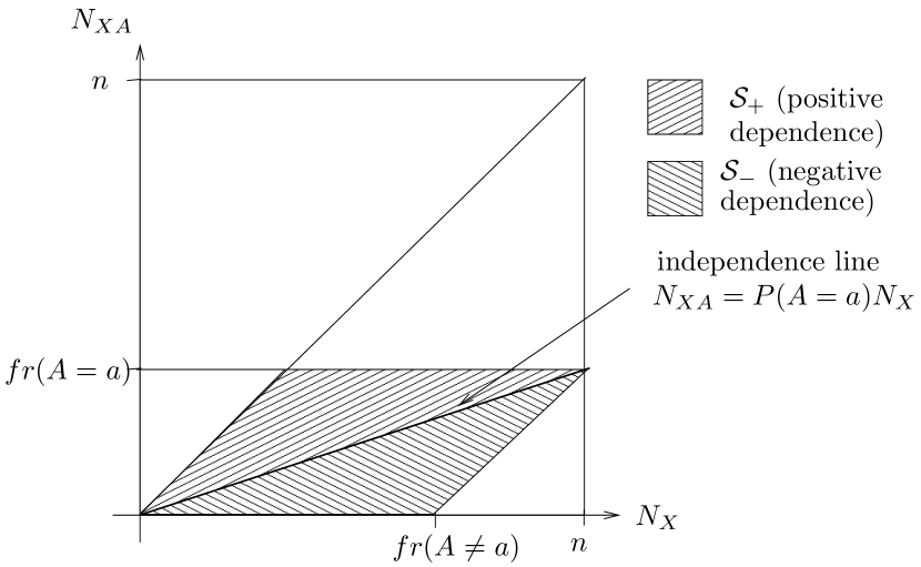
Figure 1: Two-dimensional space of absolute frequencies $N_{X}$ and $N_{XA}$, when $A=a$ is fixed. In a given data set of size $n$, all points $(m(X),m(XA=a))$ lie in patterned areas.

In any data set of size $N=n$, all possible frequency combinations $N_{X},N_{XA}$, $N_{XA}\leq N_{X}$, must lie in the triangle $\{(0,0),(n,n),(n,0)\}$. If also the consequent $A=a$ is fixed, with absolute frequency $m(A=a)$, the area of possible combinations is restricted to the patterned areas in Figure 1 . Boundary line $[(0,m(A=a)),(n,m(A=a))]$ follows from the fact that $m(XA=a)\leq m(A=a)$ and line $[(m(A\neq a),0),(n,m(A))]$ from the fact that $m(A\neq a)\geq m(XA\neq a)\Leftrightarrow m(XA=a)\geq m(X)-m(A\neq a)$. Line $[(0,0),(n,m(A=a))]$ is called the independence line, because on that line $N_{XA}=P(A=a)N_{X}$, i.e. $m(XA=a)=P(A=a)m(X)$, and the corresponding $X$ and $A=a$ are statistically independent. If the point lies above the independence line, the dependency is positive ($m(XA=a)>P(A=a)m(X)$), and below the line, it is negative ($m(XA=a)<P(A=a)m(X)$).

Figure 2: Point $(m(X),m(XA=a))$ corresponding to rule $X\rightarrow A=a$. The vertical difference $\Delta$ from the independence line measures absolute leverage, $\Delta=n\delta$.

Figure 2 shows a point $(m(X),m(XA=a))$ corresponding to rule $X\rightarrow A=a$. In this case, the dependency is positive, because $(m(X),m(XA=a))$ lies above the independence line. The slope of line $[(0,0),(n,nP(A=a|X))]$ is the rule confidence $P(A=a|X)=\frac{m(XA=a)}{m(X)}$. The vertical difference between point $(m(X),m(XA=a))$ and the independence line, marked as $\Delta$, defines the absolute leverage $\Delta=n\delta$. If the dependency is negative and the point lies below the independence line, the leverage is negative.

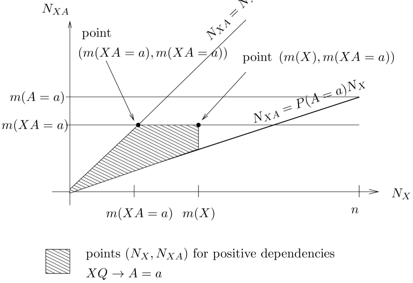
Figure 3: When a point $(m(X),m(XA=a)$, corresponding to rule $X\rightarrow A=a$, is given, the points associated to more specific positive dependency rules $XQ\rightarrow A=a$ lie in the patterned area.

Figure 3 shows how the knowledge on a rule $X\rightarrow A=a$ can be utilized to determine the possible frequency values of more specific positive dependency rules $XQ\rightarrow A=a$. Since $m(XQA=a)\leq m(XA=a)$, all points $(m(XQ),m(XQA=a))$ must lie under the line $[(0,m(XA=a)),(n,m(XA=a))]$. Because the dependencies are positive, they also have to lie above the independence line. In the next section, we will show that for a well-behaving goodness measure $M$, point $(m(XA=a),m(XA=a))$ defines an upper bound (or lower bound) for any positive dependency rule $XQ\rightarrow A=a$.

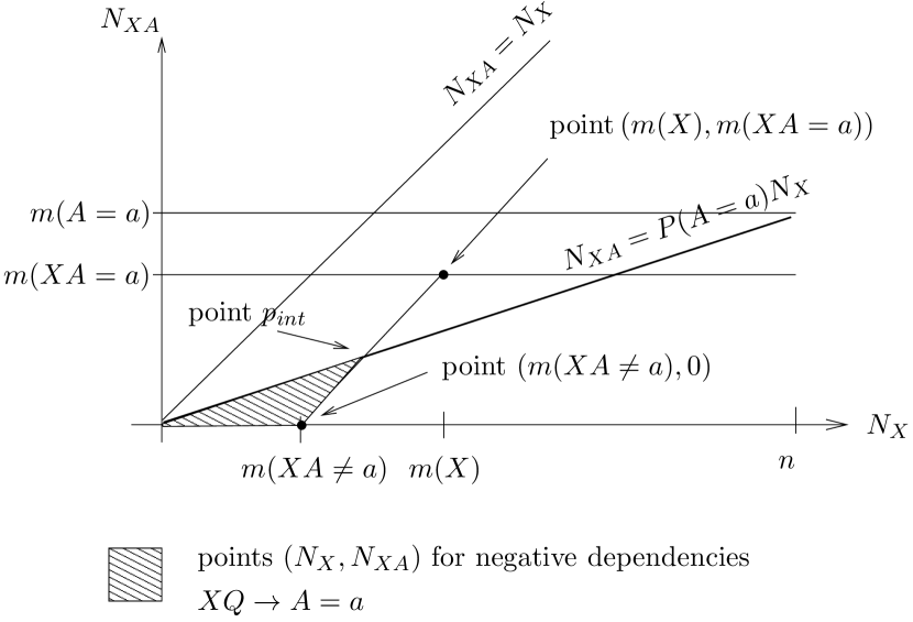
Figure 4: When a point $(m(X),m(XA=a))$, corresponding to rule $X\rightarrow A=a$, is given, the points associated to more specific negative dependency rules $XQ\rightarrow A=a$ lie in the patterned area.

Figure 4 shows the area, where all possible points for negative dependency rules $XQ\rightarrow A=a$ must lie. Once again, $m(XQA=a)\leq m(XA=a)$, and because the dependence is negative, the points must lie under the independence line. In addition, the points are restricted by line $[(m(X),m(XA=a)),(m(XA\neq a,0))]$. The reason is that $m(XQA=a)=m(XA=a)-m(X\neg QA=a)$, where $m(X\neg QA=a)\in[0,m(XA=a)]$. On the other hand, $m(XQ)=m(X)-m(X\neg QA=a)-m(X\neg QA\neq a)\leq m(X)-m(X\neg QA=a)$. So, the line contains the maximal possible values $N_{X}=m(XQ)$ and the corresponding $N_{XA}=m(XQA=a)$ for any $m(X\neg QA=a)\in[0,m(XA=a)]$. In point $(m(X),m(XA=a))$, $m(X\neg QA=a)=0$, and in point $(m(XA\neq a),0)$, $m(X\neg QA=a)=m(XA=a)$. In the following, we will show that point $(m(XA\neq a),0)$ defines an upper bound for the $M$ value of any negative dependency rule $XQ\rightarrow A=a$.

Figures 5 and 6 show the four axioms graphically. According to axioms (ii) and (iii), function $f$ increases, when it departures from the independence line either horizontally or vertically (Figure 5). According to axiom (iv), $f$ increases on lines $N_{XA}=cf_{1}N_{X}$, when $cf_{1}>P(A=a)$, and decreases on lines $m(A=a)-N_{XA}=cf_{2}(n-N_{X})$, when $cf_{2}>P(A=a)$ (Figure 6).

Figure 5: Arrows show directions where $f$ increases (Axioms (ii) and (iii)).

Figure 6: Arrows show directions where $f$ increases (Axiom (iv)).

4 Useful upper bounds

First we will note a couple of trivial properties, which follow from the definition of well-behaving measures.

Theorem 1

Let $M$ be a well-behaving, increasing measure. Let $S$ be a set of legal values, as before. When $N=n$ and $N_{A}=m(A=a)$ are fixed, $M$ is defined by function $f(N_{X},N_{XA},m(A=a),n)$.

For positive dependencies hold

• $f$ gets its maximal values in set $S$ on the border defined by points $(0,0)$, $(m(A=a),m(A=a))$, $(n,m(A=a))$.

• $f$ gets its supremum (globally maximal value) in set $S$ in point $(m(A=a),m(A=a))$.

and for negative dependencies hold

• $f$ gets its maximal values in set $S$ on the border defined by points $(0,0)$, $(m(A\neq a),0)$, $(n,m(A=a))$.

• $f$ gets its supremum in set $S$ in point $(m(A\neq a),0)$.

Proof 1

Let us first consider positive dependencies.

(i) Since $M$ is well-behaving, $f$ is an increasing function of $\delta$, when $\delta\geq 0$, in any point $N_{X}$. Therefore, it gets its maximum value on the mentioned border. (ii) When $N_{XA}=m(XA=a)$ is fixed, $M$ being well-behaving, $f$ is a decreasing function of $N_{X}$, when $N_{X}\leq\frac{n\cdot m(XA=a)}{m(A=a)}$. Therefore, $f$ is decreasing on line $[(m(A=a),m(A=a)),(n,m(A=a))]$. On the other hand, we know that for well-behaving $M$, $f(N_{X},cfN_{X},m(A=a),n)$ is increasing with $N_{X}$, when $cf>\frac{m(A=a)}{n}$. When $cf=1$, $f(N_{X},cfN_{X},m(A=a),n)$ coincides line $[(0,0),(m(A=a),m(A=a))]$. Therefore, $f$ gets its maximum value, when $N_{X}=N_{XA}=m(A=a)$.

For negative dependencies, the proof is similar. The only notable exception is that now $f$ is increasing on line $[(0,0),(m(A\neq a),0)]$ and decreasing on line $[(m(A\neq a),0),(n,m(A=a))]$.

This result can already be used for pruning in two ways. In the beginning, some of the possible consequents $A=a$ may be pruned out. Given a minimum threshold $min_{M}$, $A=a$ cannot occur in the consequent of any sufficiently good positive dependency rule, if $f(m(A=a),m(A=a),m(A=a),n)<min_{M}$. Similarly, $A=a$ cannot occur in the consequent of any sufficiently good negative dependency rule, if $f(m(A\neq a),0,m(A=a),n)<min_{M}$. We note that attribute $A$ can still occur in the antecedent of good rules. This pruning property is effective only with measures (like the mutual information), whose supremum depends on $m(A=a)$. For example, with the $\chi^{2}$ measure, the supremum is the same for all $m(A=a)$, and no pruning is possible, when nothing else is known.

The second case occurs, when only $m(X)$ is known, but $m(XA=a)$ is unknown. Now we can estimate an upper bound for both $X\rightarrow A=a$ and all its specializations $XQ\rightarrow A=a$, by substituting the best possible value for $N_{XA}$. In the case of positive dependencies, the best possible value for $N_{XA}$ is $\min\{m(X),m(A=a)\}$, and in the case of negative dependencies, it is $\max\{0,m(X)-m(A\neq a)\}$. In practice, this means that when $m(X)<m(A)$, the best possible $M$ value for positive dependence (in point $(m(A=a),m(A=a))$ cannot be achieved any more, and the effective pruning can begin. In the case of negative dependencies, the same happens, when $m(X)$ becomes $m(X)<m(A\neq a)$, and point $(m(A\neq a),0)$ is no more reachable.

The next theorem gives an upper bound for any positive or negative dependency rule, when a more general rule is already known.

Theorem 2

Let $n$ and $m(A=a)$ be fixed and $M$, $S$ and $f$ like before. Given $m(X)$ and $m(XA=a)$ and an arbitrary attribute set $Q\subseteq R\setminus(X\setminus\cup\{A\})$

• for positive dependency $XQ\rightarrow A=a$ holds $f(m(XQ),m(XQA=a),m(A=a),n)\leq f(m(XA=a),m(XA=a),m(A=a),n)$, and

• for negative dependency $XQ\rightarrow A=a$ holds $f(m(XQ),m(XQA=a),m(A=a),n)\leq f(m(XA\neq a),0,m(A=a),n)$.

Proof 2

• (Positive dependence) Figure 3 shows the area, where possible points $(m(XQ),m(XQA=a))$ for positive dependence can lie. With any $N_{X}\leq m(X)$, the maximum is achieved on the border defined by points $(0,0)$, $(m(XA=a),m(XA=a))$, and $(m(X),m(XA=a))$ ($\delta$ is maximal). On line $[(0,0),(m(XA=a),m(XA=a))]$ $f$ is increasing and on line $[(m(XA=a),m(XA=a)),(m(X),m(XA=a))]$ it is decreasing. Therefore, the global maximum is achieved in point $(m(XA=a),m(XA=a))$.

• (Negative dependence) Figure 4 shows the area, where possible points
  $(m(XQ),m(XQA=a))$ for negative dependence can lie. Once again, $f$ gets its maximal value for any $N_{X}$, when $-\delta$ is maximal. Therefore, the maximum must lie on the border defined by points $(0,0)$, $(m(XA\neq a),0)$, and the intersection point $p_{int}$. On line $[(0,0),(m(XA\neq a),0))]$, $f$ is increasing, and the maximal value is achieved in point $(m(XA\neq a),0)$. Therefore, it suffices to show that $f$ gets its maximum on line $[p_{int},(m(XA\neq a),0)]$ in the same point, $(m(XA\neq a),0)$.

  Figure 7 shows the proof idea. For every point $p_{1}$ on line $[p_{int},(m(XA\neq a),0)]$, we can define a line of form $m(A=a)-N_{XA}=cf_{2}(n-N_{X})$, which goes through $p_{1}$. Because $p_{1}$ is under the independence line, $cf_{2}>P(A=a)$, and line $m(A=a)-N_{XA}=cf_{2}(n-N_{X})$ intersects $N_{X}$-axis in some point $p_{2}$ in the interval $[(0,0),(m(XA\neq a),0)]$. According to the definition of well-behaving measures, $f$ is decreasing on line $m(A=a)-N_{XA}=cf_{2}(n-N_{X})$, and therefore $f$ gets a better value in point $p_{2}$ than in point $p_{1}$. On the other hand, we already know that $f$ gets a better value in $(m(XA\neq a),0)$ than any point $p_{2}$. Therefore, $f$ must get its upper bound in point $(m(XA\neq a),0)$.

Figure 7: Proof idea. Function $f$ is better in $p_{2}$ than in $p_{1}$ and better in point $(m(XA\neq a),0)$ than in $p_{2}$.

These upper bounds enable more effective pruning than Theorem 1, because now pruning is possible even if $m(X)>m(A=a)$ or $m(X)>m(A\neq a)$. The upper bounds are also tight in the sense that there can be rules $XQ\rightarrow A$, which reach the upper bound values.

5 Conclusions

We have formalized the classical axioms for proper goodness measures and extended them to to cover both positive and negative dependency rules. We have shown that all such well-behaving goodness measures achieve their upper bounds in the same points of the search space. This is an important results, because it means that the same generic search algorithm can be applied for a large variety of commonly used goodness measures.

Appendix A Example proofs for the good behaviour of common goodness measures

In the following, we show that the $\chi^{2}$-measure, mutual information, two versions of the $z$-score (e.g. [2, 3, 1]), and the $J$-measure [7] are well-behaving measures. The first two measures are defined for both positive and negative dependencies, while the last three are defined only for positive dependencies.

Theorem 3

Let $S\subseteq N^{4}$ be defined by constraints $0<N$, $0<N_{X}<N$, $0<N_{A}<N$, and $0\leq N_{XA}\leq\min\{N_{X},N_{A}\}$. Measure $M$ is well-behaving, if it is defined by function

• $\chi^{2}(N_{X},N_{XA},N_{A},N)=\frac{N(NN_{XA}-N_{X}N_{A})^{2}}{N_{X}(N-N_{X})N_{A}(N-N_{A})}$,

• $MI(N_{X},N_{XA},N_{A},N)=N_{XA}\log\frac{N\cdot N_{XA}}{N_{X}N_{A}}+(N_{X}-N_{XA})\log\frac{N\cdot(N_{X}-N_{XA})}{N_{X}(N-N_{A})}$
  $+(N_{A}-N_{XA})\log\frac{N\cdot(N_{A}-N_{XA})}{(N-N_{X})N_{A}}+(N-N_{X}-N_{A}+N_{XA})\log\frac{N\cdot(N-N_{X}-N_{A}+N_{XA})}{(N-N_{X})(N-N_{A})}$,

• $z_{1}(N_{X},N_{XA},N_{A},N)=\frac{\sqrt{N}(NN_{XA}-N_{X}N_{A})}{\sqrt{N_{X}N_{A}(N^{2}-N_{X}N_{A})}},$ when $NN_{XA}>N_{X}N_{A}$, and 0, otherwise,

• $z_{2}(N_{X},N_{XA},N_{A},N)=\frac{NN_{XA}-N_{X}N_{A}}{\sqrt{N_{X}N_{A}(N-N_{A})}},$ when $NN_{XA}>N_{X}N_{A}$, and 0, otherwise, and

• $J(N_{X},N_{XA},N_{A},N)=N_{XA}\log(\frac{N_{XA}}{N_{A}})+(N_{X}-N_{XA})\log(\frac{N_{X}-N_{XA}}{N-N_{A}})-N_{X}\log(\frac{N_{X}}{N})$, when $NN_{XA}>N_{X}N_{A}$, and 0, otherwise.

Proof 3

In the proofs, we assume that $N=n$ is fixed. We will simplify the functions by substituting $P(XA)=\frac{N_{XA}}{N}$, $P(X)=\frac{N_{X}}{N}$, $P(A)=\frac{N_{A}}{N}$.

• Conditions (i) and (ii): For $\chi^{2}$ the alternative expression is

  $$f_{2}(P(X),\delta,P(A),n)=\frac{n\delta^{2}}{P(X)(1-P(X))P(A)(1-P(A))}.$$

  The derivative with respect to $\delta$ is

  $$f_{2}^{\prime}=\frac{2n\delta}{P(X)(1-P(X))P(A)(1-P(A))},$$

  which satisfies the conditions (i) and (ii).

  Condition (iii): When $P(XA)$, $P(A)$, and $n$ are fixed, $f$ can be expressed as

  $$f(P(X),P(XA),P(A),n)=\frac{n}{P(A)(1-P(A))}g(P(X)),$$

  where $g(P(X))=\frac{(P(XA)-P(X)P(A))^{2}}{P(X)(1-P(X))}$. The first factor is constant, and therefore it is sufficient to differentiate $g(P(X))$ with respect to $P(X)$.

  $$g^{\prime}(P(X))=\frac{-2P(XA)P(X)^{2}P(A)+P(X)^{2}P(A)^{2}-P(XA)^{2}+2P(X)P(XA)^{2}}{P(X)^{2}(1-P(X))^{2}}.$$

  The denominator is $[P(XA)-P(X)P(A)][-P(X)P(A)-P(XA)+2P(X)P(XA)]=[P(XA)-P(X)P(A)][P(X)(P(XA)-P(A))+P(XA)(P(X)-1)]$. The first factor is leverage $\delta$ and the second factor is always negative. Therefore, $g^{\prime}<0$, when $\delta>0$, and $g^{\prime}>0$, when $\delta<0$.

  Condition (iv): Let as first check the case, where $N_{XA}=cf_{1}N_{X}$. Now $f$ becomes

  $$f(P(X),cf_{1}P(X),P(A),n)=\frac{nP(X)(cf_{1}-P(A))^{2}}{P(A)(1-P(A))(1-P(X))}.$$

  This is clearly an increasing function of $P(X)$, when $cf_{1}\neq P(A)$. Let us then check case $N_{XA}=m(A)-cf_{2}(n-N_{X})$. Now $f$ becomes

  $$f(P(X),P(A)-cf_{2}(1-P(X)),P(A),n)=\frac{n(1-P(X))(P(A)-cf_{2})^{2}}{P(X)P(A)(1-P(A))}.$$

  This is clearly a decreasing function of $P(X)$, when $cf_{2}\neq P(A)$.

• In mutual information, the base of the logarithm is not defined, but usually it is assumed to be 2. However, transformation to the natural logarithm causes only an extra term +1, which disappears in differentiation. Therefore we will use the natural logarithms for simplicity. We recall that the derivative of a term of form $g(x)\ln(g(X))$ is $g^{\prime}(x)\ln(g(x))+g^{\prime}(x)$.

  Condition (i) and (ii): $MI$ can be expressed as function $f_{2}$:

  $$f_{2}(P(X),\delta,P(A),n)=n[(P(X)P(A)+\delta)\ln(P(X)P(A)+\delta)+(P(X)(1-P(A))-\delta)\ln(P(X)\\ (1-P(A))-\delta)+((1-P(X))P(A)-\delta)\ln((1-P(X))P(A)-\delta)+((1-P(X))(1-P(A))+\delta)\\ \ln((1-P(X))(1-P(A))+\delta)-P(A)\ln(P(A))-(1-P(A))\ln(1-P(A))-P(X)\ln(P(X))\\ -(1-P(X))\ln(1-P(X))].$$

  The derivative of $f_{2}$ with respect to $\delta$ is

  $$f_{2}^{\prime}=n\ln\left(\frac{(P(X)P(A)+\delta)((1-P(X))(1-P(A))+\delta)}{((P(X)(1-P(A))-\delta)((1-P(X))P(A)-\delta)}\right).$$

  This is the same as $n$ times the logarithm of the odds ratio $odds$, for which holds $odds=1$, when $\delta=0$, $odds>1$, when $\delta>0$, and $odds<1$, when $\delta<0$. Therefore, the logarithm is zero, when $\delta=0$, negative, when $\delta<0$, and positive, when $\delta>0$.

  Condition (iii): When $P(XA)$, $P(A)$, and $n$ are fixed, $f$ can be expressed as

  $$g(P(X))=n[P(XA)\ln(P(XA))+(P(X)-P(XA))\ln(P(X)-P(XA))+(P(A)-P(XA))\\ \ln(P(A)-P(XA))+(1-P(X)-P(A)+P(XA))\ln(1-P(X)-P(A)+P(XA))-P(A)\\ \ln(P(A))-(1-P(A))\ln(1-P(A))-P(X)\ln(P(X))-(1-P(X))\ln(1-P(X))].$$

  The derivative of $g$ with respect to $P(X)$ is

  $$g^{\prime}=n\ln\left(\frac{(P(X)-P(XA))(1-P(X))}{(1-P(X)-P(A)+P(XA))P(X)}\right).$$

  Since $q=\frac{(P(X)-P(XA))(1-P(X))}{(1-P(X)-P(A)+P(XA))P(X)}=1$, when $P(XA)=P(X)P(A)$, $q>1$, when $P(XA)<P(X)P(A)$, and $q<1$, when $P(XA)>P(X)P(A)$, the logarithm is zero, when $X$ and $A=a$ are independent, negative, when $X$ and $A=a$ are positively dependent, and positive, when $X$ and $A=a$ are negatively dependent.

  Condition (iv): When $N_{XA}=cf_{1}N_{X}$, $f$ becomes

  $$f(P(X),cf_{1}P(X),P(A),n)=n[P(X)cf_{1}\ln(P(X)cf_{1})+P(X)(1-cf_{1})\ln(P(X)(1-cf_{1}))\\ +(P(A)-P(X)cf_{1})\ln(P(A)-P(X)cf_{1})+(1-P(X)-P(A)+P(X)cf_{1})\ln(1-P(X)-P(A)\\ +P(X)cf_{1})-P(X)\ln P(X)-(1-P(X))\ln(1-P(X))-P(A)\ln P(A)-(1-P(A))\ln(1-P(A))].$$

  The derivative of $f$ is

  $$f^{\prime}=n[cf_{1}\ln(P(X)cf_{1})+(1-cf_{1})\ln(P(X)(1-cf_{1}))-cf_{1}\ln(P(A)-P(X)cf_{1})-(1-cf_{1})\\ \ln(1-P(X)-P(A)+P(X)cf_{1})-\ln(P(X))+\ln(1-P(X))].$$

  We should show that $f^{\prime}>0$, when $cf_{1}>P(A)$. To find the lowest value of $f^{\prime}$, we set $g(cf_{1})=f^{\prime}(P(X))$ and differentiate $g$ with respect to $cf_{1}$.

  $$g^{\prime}(cf_{1}) =n\left[\ln\left(\frac{P(X)cf_{1}(1-P(X)-P(A)+P(X)cf_{1})}{P(X)(1-cf_{1})(P(A)-P(X)cf_{1})}\right)+\frac{P(X)cf_{1}}{P(A)-P(X)cf_{1}}\right.$$

  $$\left.-\frac{P(X)(1-cf_{1})}{1-P(X)-P(A)+P(X)cf_{1}}\right]$$

  $$=n\left[\ln\left(\frac{P(XA)P(\neg X\neg A)}{P(X\neg A)P(\neg XA)}\right)+\frac{P(XA)P(\neg X\neg A)-P(\neg XA)P(X\neg A)}{P(\neg XA)P(X\neg A)}\right]$$

  $$=n\left[\ln(odds)+\frac{\delta}{P(\neg XA)P(X\neg A)}\right].$$

  The first term is the logarithm of the odds ratio, which is $>0$, when $\delta>0$. So $g^{\prime}>0$, when $\delta>0$. Therefore, $g$ is an increasing function of $cf_{1}$ and gets its minimal value, when $\delta=0$ and $cf_{1}=P(A)$. When we substitute this to $f^{\prime}$, we get $f^{\prime}=\ln(1)=0$. This is the minimal value of $f^{\prime}$, which is achieved only, when $\delta=0$; otherwise $f^{\prime}>0$, as desired.

  Let us then check case $N_{XA}=m(A)-cf_{2}(n-N_{X})$. Now $P(XA)=P(A)-cf_{2}(1-P(X))$, $P(X\neg A)=P(X)(1-cf_{2})-P(A)+cf_{2}$, $P(\neg XA)=cf_{2}(1-P(X))$, $P(\neg X\neg A)=(1-P(X))(1-cf_{2})$, and $f$ becomes

  $$f(P(X),P(A)-cf_{2}(1-P(X)),P(A),n)=\\ n[(P(A)-cf_{2}(1-P(X)))\ln(P(A)-cf_{2}(1-P(X)))+(P(X)(1-cf_{2})-P(A)+cf_{2})\ln(P(X)\\ (1-cf_{2})-P(A)+cf_{2})+cf_{2}(1-P(X))\ln(cf_{2}(1-P(X)))+(1-P(X))(1-cf_{2})\ln((1-P(X))\\ (1-cf_{2}))-P(X)\ln P(X)-(1-P(X))\ln(1-P(X))-P(A)\ln(P(A))-(1-P(A))\ln(1-P(A))]\\ =n[(P(A)-cf_{2}(1-P(X)))\ln(P(A)-cf_{2}(1-P(X)))+(P(X)(1-cf_{2})-P(A)+cf_{2})\ln(P(X)\\ (1-cf_{2})-P(A)+cf_{2})+cf_{2}(1-P(X))\ln(cf_{2})+(1-P(X))(1-cf_{2})\ln(1-cf_{2})-P(X)\ln P(X)\\ -P(A)\ln(P(A))-(1-P(A))\ln(1-P(A))]$$

  The derivative of $f$ with respect to $P(X)$ is

  $$f^{\prime}=n[cf_{2}\ln\frac{P(A)-cf_{2}(1-P(X))}{cf_{2}}+(1-cf_{2})\ln\frac{P(X)(1-cf_{2})-P(A)+cf_{2}}{1-cf_{2}}\\ -\ln(P(X))].$$

  We should show that $f^{\prime}<0$, when $cf_{2}>P(A)$. To find the largest value of $f^{\prime}$, we set $g(cf_{2})=f^{\prime}(P(X))$ and differentiate $g$ with respect to $cf_{2}$.

  $$g^{\prime}(cf_{2}) =n\left[\ln\left(\frac{P(A)-cf_{2}(1-P(X))}{cf_{2}}\right)-\ln\left(\frac{P(X)-P(A)+cf_{2}(1-P(X))}{1-cf_{2}}\right)\right.$$

  $$\left.-\frac{P(A)}{P(A)-cf_{2}(1-P(X))}+\frac{1-P(A)}{P(X)-P(A)+cf_{2}(1-P(X))}\right]$$

  $$=n\left[\ln\left(\frac{P(XA)(1-cf_{2})}{cf_{2}P(X\neg A)}\right)-\frac{P(A)}{P(XA)}+\frac{1-P(A)}{P(X\neg A)}\right].$$

  Because the dependence is negative, $-P(XA)>-P(X)P(A)$ and $P(X)(1-P(A))<P(X\neg A)$. Therefore, the sum of the last two terms is $<0$. The first term becomes $\ln(odds)$, when we substitute $cf_{2}=P(A|\neg X)$. For negative dependence, also $\ln(odds)<0$, and therefore $g^{\prime}<0$. Because $g$ is decreasing with $cf_{2}$, $f^{\prime}$ gets its maximum value, when $cf_{2}$ is minimal, i.e. $P(A)$. When we substitute this to $f^{\prime}$, it becomes $f^{\prime}=0$. This is the maximal value of $f^{\prime}$, which is achieved only when $cf_{2}=P(A)$ and $\delta=0$. Otherwise, $f^{\prime}<0$, as desired.

• Now it is enough to check the conditions only for the positive dependence.

  Conditions (i) and (ii): $z_{1}$ can be expressed as

  $$f_{2}(P(X),\delta,P(A),n)=\frac{\sqrt{n}\delta}{\sqrt{P(X)P(A)(1-P(X)P(A))}},$$

  when $\delta>0$, and $f_{2}=0$, otherwise. This is clearly an increasing function of $\delta$ and gets its minimum value $0$, when $\delta\leq 0$.

  Condition (iii): When $P(XA)$, $P(A)$, and $n$ are fixed, $f$ can be expressed as

  $$f(P(X),P(XA),P(A),n)=\frac{\sqrt{n}}{\sqrt{P(A)}}g(P(X)),$$

  where $g(P(X))=\frac{P(XA)-P(X)P(A)}{\sqrt{P(X)(1-P(X)P(A))}}$. The derivative of $g$ with respect to $P(X)$ is

  $$g^{\prime} =\frac{-2P(X)P(A)(1-P(X)P(A))-(P(XA)-P(X)P(A))(1-2P(X)P(A))}{2(P(X)(1-P(X)P(A)))^{\frac{3}{2}}}$$

  $$=\frac{-P(X)P(A)(1-P(XA))-P(XA)(1-P(X)P(A))}{2(P(X)(1-P(X)P(A)))^{\frac{3}{2}}}.$$

  Because $P(X)P(A)<1$ and $P(XA)\leq 1$, $g^{\prime}<0$ always.

  Condition (iv): When $N_{XA}=cf_{1}N_{X}$, $f$ becomes

  $$f(P(X),cf_{1}P(X),P(A),n)=\frac{\sqrt{nP(X)}(cf_{1}-P(A))}{\sqrt{P(A)(1-P(X)P(A)})},$$

  which is clearly an increasing function of $P(X)$, when $cf_{1}\geq P(A)$.

• Conditions (i) and (ii): $z_{2}$ can be expressed as

  $$f_{2}(P(X),\delta,P(A),n)=\frac{\sqrt{n}\delta}{\sqrt{P(X)P(A)(1-P(A))}},$$

  when $\delta>0$, and $f_{2}=0$, otherwise. This is clearly an increasing function of $\delta$ and gets its minimum value $0$, when $\delta\leq 0$.

  Condition (iii): When $P(XA)$, $P(A)$, and $n$ are fixed, $f$ can be expressed as

  $$f(P(X),P(XA),P(A),n)=\frac{\sqrt{n}}{\sqrt{P(A)(1-P(A))}}g(P(X)),$$

  where $g(P(X))=\frac{P(XA)-P(X)P(A)}{\sqrt{P(X)}}$. The derivative of $g$ with respect to $P(X)$ is

  $$g^{\prime}(P(X))=\frac{-P(X)P(A)-P(XA)}{2P(X)^{\frac{3}{2}}},$$

  which is $<0$ always.

  Condition (iv): When $P(XA)=cf_{1}P(X)$, $f$ becomes

  $$f(P(X),cf_{1}P(X),P(A),n)=\frac{\sqrt{nP(X)}(cf_{1}-P(A))}{\sqrt{P(A)(1-P(A))}},$$

  which is clearly an increasing function of $P(X)$, when $cf_{1}\geq P(A)$.

• Like in the mutual information, we will use the natural logarithm for simplicity.

  Conditions (i) and (ii): $J$ can be expressed as

  $$f_{2}(P(X),\delta,P(A),n)=n\left[(P(X)P(A)+\delta)\ln\left(\frac{P(X)P(A)+\delta}{P(A)}\right)\right.\\ \left.+(P(X)(1-P(A))-\delta)\ln\left(\frac{P(X)(1-P(A))-\delta}{(1-P(A))}\right)-P(X)\ln(P(X))\right].$$

  The derivative of $f_{2}$ with respect to $\delta$ is

  $$f_{2}^{\prime} =n\left[\ln\left(\frac{P(X)P(A)+\delta}{P(A)}\right)-\ln\left(\frac{P(X)(1-P(A))-\delta}{(1-P(A))}\right)-\ln(P(X))\right]$$

  $$=n\ln\left(\frac{(P(X)P(A)+\delta)(1-P(A))}{(P(X)(1-P(A))-\delta)P(X)P(A)}\right).$$

  The argument of the logarithm is 1, if $\delta=0$, and otherwise it is $>1$. Therefore, $f_{2}^{\prime}\geq 0$, when $\delta\geq 0$.

  Condition (iii): When $P(XA)$, $P(A)$, and $n$ are fixed, $f$ can be expressed as

  $$g(P(X))=n[P(XA)\ln\left(\frac{P(XA)}{P(A)}\right)+(P(X)-P(XA))\ln\left(\frac{P(X)-P(XA)}{(1-P(A))}\right)\\ -P(X)\ln(P(X))].$$

  The derivative of $g$ with respect to $P(X)$ is

  $$g^{\prime}=n[\ln\left(\frac{P(X)-P(XA)}{(1-P(A))}\right)-\ln(P(X))]=n\ln\left(\frac{P(X)-P(XA)}{P(X)(1-P(A))}\right).$$

  The argument of the logarithm is $<1$ and thus $g^{\prime}<0$, if there is a positive dependency.

  Condition (iv): When $N_{XA}=cf_{1}N_{X}$, $f$ becomes

  $$f(P(X),cf_{1}P(X),P(A),n)=\\ n\left[P(X)cf_{1}\ln\left(\frac{P(X)cf_{1}}{P(A)}\right)+P(X)(1-cf_{1})\ln\left(\frac{P(X)(1-cf_{1})}{(1-P(A))}\right)-P(X)\ln(P(X))\right].$$

  The derivative of $f$ with respect to $P(X)$ is

  $$f^{\prime} =n\left[cf_{1}\ln\left(\frac{P(X)cf_{1}}{P(A)}\right)+(1-cf_{1})\ln\left(\frac{P(X)(1-cf_{1})}{(1-P(A))}\right)-\ln(P(X))\right]$$

  $$=n\left[cf_{1}\ln\left(\frac{cf_{1}(1-P(A))}{(1-cf_{1})P(A)}\right)+\ln\left(\frac{1-cf_{1}}{(1-P(A))}\right)\right].$$

  We should show that $f^{\prime}>0$, when $cf_{1}>P(A)$. To find the lowest value of $f^{\prime}$, we set $g(cf_{1})=f^{\prime}(P(X))$ and derivative $g$ with respect to $cf_{1}$.

  $$g^{\prime}(cf_{1})=n\ln\left(\frac{cf_{1}(1-P(A))}{(1-cf_{1})P(A)}\right).$$

  Clearly $g^{\prime}=0$, if $cf_{1}=P(A)$, and $g^{\prime}>0$, if $cf_{1}>P(A)$. When we substitute the minimum value $cf_{1}=P(A)$ to $f^{\prime}$, we get $f^{\prime}=n[P(A)\ln(1)+\ln(1)]=0$. When $cf_{1}>P(A)$, $f^{\prime}>0$, and $f$ is an increasing function of $P(X)$.

References

- [1] D. Bruzzese and C. Davino. Visual post-analysis of association rules. Journal of Visual Languages & Computing, 14:621–635, December 2003.
- [2] W. Hämäläinen and M. Nykänen. Efficient discovery of statistically significant association rules. In Proceedings of the 8th IEEE International Conference on Data Mining (ICDM 2008), pages 203–212, 2008.
- [3] S. Lallich, O. Teytaud, and E. Prudhomme. Association rule interestingness: Measure and statistical validation. In F. Guillet and H.J. Hamilton, editors, Quality Measures in Data Mining, volume 43 of Studies in Computational Intelligence, pages 251–275. Springer, 2007.
- [4] J.A. Major and J.J. Mangano. Selecting among rules induced from a hurricane database. Journal of Intelligent Information Systems, 4:39–52, January 1995.
- [5] S. Morishita and J. Sese. Transversing itemset lattices with statistical metric pruning. In Proceedings of the nineteenth ACM SIGMOD-SIGACT-SIGART symposium on Principles of database systems (PODS’00), pages 226–236. ACM Press, 2000.
- [6] G. Piatetsky-Shapiro. Discovery, analysis, and presentation of strong rules. In G. Piatetsky-Shapiro and W.J. Frawley, editors, Knowledge Discovery in Databases, pages 229–248. AAAI/MIT Press, 1991.
- [7] P. Smyth and R.M. Goodman. An information theoretic approach to rule induction from databases. IEEE Transactions on Knowledge and Data Engineering, 4(4):301–316, 1992.