Propagation of quantum correlations after a quench in the Mott-insulator regime of the Bose-Hubbard model

Abstract

We study a quantum quench in the Bose-Hubbard model where the tunneling rate $J$ is suddenly switched from zero to a finite value in the Mott regime. In order to solve the many-body quantum dynamics far from equlibrium, we consider the reduced density matrices for a finite number of lattice sites and split them up into on-site density operators, i.e., the mean field, plus two-point and three-point correlations etc. Neglecting three-point and higher correlations, we are able to numerically simulate the time-evolution of the on-site density matrices and the two-point quantum correlations (e.g., their effective light-cone structure) for a comparably large number ${\cal O}(10^{3})$ of lattice sites.

Research

1 Introduction

The exponential growth of the underlying Hilbert space is one of the main reasons for our limited ability to simulate quantum many-body systems. In contrast to classical many-particle systems, it is not sufficient to treat the state of each particle or lattice site separately – one has to consider the quantum correlations (entanglement) as well. If these quantum correlations obey certain properties, for example if they are sufficiently short-ranged, there are quite efficient methods for approximating the quantum state of the system, such as matrix-product states [2, 3, 4, 5]. However, in typical non-equilibrium situations [6, 7, 8, 9, 10, 11, 12, 13, 14, 15, 16] these quantum correlations tend to spread [17, 18, 19, 20, 21, 22, 23, 24, 25, 26, 27] and thus are not short-ranged after some time – which is the reason why these methods typically break down in such cases eventually. In the following, we present an alternative method which fully incorporates quantum correlations between pairs of lattice sites at arbitrary distances. The price we have to pay is the neglect of genuine three-point (and higher) correlations. However, comparison with exact numerical diagonalization (for small systems) reveals that this is a reasonable approximation. Even though the method we shall present can be applied to quite general lattice systems, we are going to focus on the Bose-Hubbard model, because the non-equlibrium many-body quantum dynamics in this system can be tested in high-precision experiments using ultra-cold atoms in optical lattices [28, 29, 30].

2 Bose-Hubbard model

We consider a system of bosons with local interactions in a lattice described by the Bose-Hubbard Hamiltonian

$$\hat{H}=-\frac{J}{Z}\sum_{\mu_{1}\mu_{2}}T_{\mu_{1}\mu_{2}}\hat{b}^{\dagger}_{\mu_{1}}\hat{b}_{\mu_{2}}+\frac{U}{2}\sum_{\mu}\hat{n}_{\mu}(\hat{n}_{\mu}-1)\;,$$ (1)

where $J$ is the tunneling rate for the nearest neighbors and $U>0$ is the interaction parameter. The creation and annihilation operators $\hat{b}^{\dagger}_{\mu_{1}}$ and $\hat{b}_{\mu_{2}}$ at the lattice sites $\mu_{1}$ and $\mu_{2}$, respectively, satisfy the standard bosonic commutation relations, and $\hat{n}_{\mu}=\hat{b}^{\dagger}_{\mu}\hat{b}_{\mu}$ is the particle-number operator. The lattice structure is encoded in the adjacency matrix $T_{\mu_{1}\mu_{2}}$ which equals unity if the sites labeled by $\mu_{1}$ and $\mu_{2}$ are tunneling neighbors (i.e., if a particle can hop from $\mu_{1}$ to $\mu_{2}$) and zero otherwise. The number of tunneling neighbors at a given site $\mu_{1}$ yields the coordination number $Z=\sum_{\mu_{2}}T_{\mu_{1}\mu_{2}}$. (We assume a translationally invariant lattice with periodic boundary conditions).

In order to study the time evolution of the system after a sudden change of the parameter $J$, we consider the density matrix describing the quantum state of the complete lattice which obeys the von Neumann equation ($\hbar=1$)

$$i\partial_{t}\hat{\rho}=\left[\hat{H},\hat{\rho}\right]\;.$$ (2)

Then we introduce a set of $\ell$-point reduced density matrices for the sites $\mu_{1}\mu_{2}\cdots\mu_{\ell}$ by tracing over all other sites:

$$\hat{\rho}_{\mu_{1}\mu_{2}\cdots\mu_{\ell}}={\rm tr}_{\not\mu_{1}\not\mu_{2}\cdots\not\mu_{\ell}}\{\hat{\rho}\}\;.$$ (3)

These reduced density matrices can be split up into their correlated parts $\hat{\rho}_{\mu_{1}\mu_{2}\cdots\mu_{\ell}}^{\rm corr}$ plus all possible products of reduced density matrices for single lattice sites and the correlated parts of the reduced density matrices for smaller number of sites – such that the total number of sites for the terms within each product equals to $\ell$. For instance, the correlated parts of the two-point and three-point reduced density matrices are in anology with the cumulant expansion given by

$$\hat{\rho}_{\mu_{1}\mu_{2}}^{\rm corr} = \hat{\rho}_{\mu_{1}\mu_{2}}-\hat{\rho}_{\mu_{1}}\hat{\rho}_{\mu_{2}}$$

$$\hat{\rho}_{\mu_{1}\mu_{2}\mu_{3}}^{\rm corr} = \hat{\rho}_{\mu_{1}\mu_{2}\mu_{3}}-\hat{\rho}_{\mu_{1}\mu_{2}}^{\rm corr}\hat{\rho}_{\mu_{3}}-\hat{\rho}_{\mu_{1}\mu_{3}}^{\rm corr}\hat{\rho}_{\mu_{2}}-\hat{\rho}_{\mu_{2}\mu_{3}}^{\rm corr}\hat{\rho}_{\mu_{1}}-\hat{\rho}_{\mu_{1}}\hat{\rho}_{\mu_{2}}\hat{\rho}_{\mu_{3}}\;.$$

Inserting this split into the von Neumann equation (2) yields the equations of motion for the reduced density matrices $\rho_{\mu_{1}}$ for single lattice sites (i.e., the on-site matrices) and the correlated parts $\hat{\rho}_{\mu_{1}\mu_{2}\cdots\mu_{\ell}}^{\rm corr}$, which were already derived in Ref. [31]. The equation for the on-site matrix $\hat{\rho}_{\mu_{1}}$ reads

$$i\partial_{t}\hat{\rho}_{\mu_{1}} = \left[\hat{H}_{\mu_{1}},\hat{\rho}_{\mu_{1}}\right]+\frac{1}{Z}\sum_{\mu_{2}\neq\mu_{1}}{\rm tr}_{\mu_{2}}\left\{\hat{H}_{\mu_{1}\mu_{2}}+\hat{H}_{\mu_{2}\mu_{1}},\hat{\rho}_{\mu_{1}\mu_{2}}^{\rm corr}+\hat{\rho}_{\mu_{1}}\hat{\rho}_{\mu_{2}}\right\}\,,$$ (4)

where $\hat{H}_{\mu}=(U/2)\hat{n}_{\mu}(\hat{n}_{\mu}-1)$ and $\hat{H}_{\mu_{1}\mu_{2}}=-JT_{\mu_{1}\mu_{2}}\hat{b}^{\dagger}_{\mu_{1}}\hat{b}_{\mu_{2}}$ are the local and non-local parts of the Hamiltonian.

The analogous equation for the two-point correlators $\hat{\rho}_{\mu_{1}\mu_{2}}^{\rm corr}$ contains the on-site matrices $\hat{\rho}_{\mu_{1}}$, but also the three-point correlations $\hat{\rho}_{\mu_{1}\mu_{2}\mu_{3}}^{\rm corr}$. In the following, we assume that we can neglect these three-point correlations – which is the main assumption of our method. The quality of this approximation will be discussed in the next section. With this assumption, we obtain the approximate equation for $\hat{\rho}_{\mu_{1}\mu_{2}}^{\rm corr}$:

$$i\partial_{t}\hat{\rho}_{\mu_{1}\mu_{2}}^{\rm corr} = \left[\hat{H}_{\mu_{1}},\hat{\rho}_{\mu_{1}\mu_{2}}^{\rm corr}\right]+\frac{1}{Z}\left[\hat{H}_{\mu_{1}\mu_{2}},\hat{\rho}_{\mu_{1}\mu_{2}}^{\rm corr}+\hat{\rho}_{\mu_{1}}\hat{\rho}_{\mu_{2}}\right]$$

$$- \frac{1}{Z}\hat{\rho}_{\mu_{1}}{\rm tr}_{\mu_{1}}\left\{\left[\hat{H}_{\mu_{1}\mu_{2}}+\hat{H}_{\mu_{2}\mu_{1}},\hat{\rho}_{\mu_{1}\mu_{2}}^{\rm corr}+\hat{\rho}_{\mu_{1}}\hat{\rho}_{\mu_{2}}\right]\right\}$$

$$+ \frac{1}{Z}\sum_{\mu_{3}\neq\mu_{1},\mu_{2}}{\rm tr}_{\mu_{3}}\left\{\left[\hat{H}_{\mu_{1}\mu_{3}}+\hat{H}_{\mu_{3}\mu_{1}},\hat{\rho}_{\mu_{1}\mu_{2}}^{\rm corr}\hat{\rho}_{\mu_{3}}+\hat{\rho}_{\mu_{2}\mu_{3}}^{\rm corr}\hat{\rho}_{\mu_{1}}\right]\right\}$$

$$+ (\mu_{1}\leftrightarrow\mu_{2})\;.$$

As a consequence, the two equations (4) and (2) form an approximate closed set of coupled non-linear equations, which we solve numerically.

In the present work, we are interested in the dynamics of the system within the Mott-insulator phase. Due to the fact that the $U(1)$-symmetry is not broken, $\hat{\rho}_{\mu}$ is diagonal in the basis of the local Fock states $|n\rangle_{\mu}$ and the equation of motion (4) simplifies in this basis to

$$i\partial_{t}\langle\hat{O}_{\mu_{1}}^{n_{1}n_{1}}\rangle=-\frac{J}{Z}\sum_{\mu_{2}}T_{\mu_{1}\mu_{2}}\left(\sqrt{n_{1}}\,\psi_{\mu_{1}\mu_{2}}^{n_{1},n_{1}-1}-\sqrt{n_{1}+1}\,\psi_{\mu_{1}\mu_{2}}^{n_{1}+1,n_{1}}-{\rm c.c.}\right)\,,$$ (6)

where $\hat{O}_{\mu}^{n_{1}n_{2}}=|n_{1}\rangle_{\mu}\langle n_{2}|$ and we use the notations

$$\langle\hat{O}_{\mu}^{n_{1}n_{2}}\rangle = {\rm tr}\left\{\hat{\rho}_{\mu}\hat{O}_{\mu}^{n_{1}n_{2}}\right\}\;,$$ (7)

$$\langle\hat{O}_{\mu_{1}}^{n_{1}n_{2}}\hat{O}_{\mu_{2}}^{n_{3}n_{4}}\rangle^{\rm corr} = {\rm tr}\left\{\hat{\rho}_{\mu_{1}\mu_{2}}^{\rm corr}\hat{O}_{\mu_{1}}^{n_{1}n_{2}}\hat{O}_{\mu_{2}}^{n_{3}n_{4}}\right\}\;,$$

$$\psi_{\mu_{1}\mu_{2}}^{n_{1}n_{2}} = \langle\hat{O}^{n_{1}n_{2}}_{\mu_{1}}\hat{b}_{\mu_{2}}\rangle^{\rm corr}=\sum_{n_{3}=0}^{\infty}\sqrt{n_{3}+1}\langle\hat{O}^{n_{1}n_{2}}_{\mu_{1}}\hat{O}^{n_{3},n_{3}+1}_{\mu_{2}}\rangle^{\rm corr}\;.$$

Note that in the regime we are interested in (vanishing order parameter: $\langle\hat{b}_{\mu}\rangle=0$), $\langle\hat{O}_{\mu}^{n_{1}n_{2}}\rangle$ vanishes for $n_{1}\neq n_{2}$. The diagonal terms $\langle\hat{O}_{\mu}^{nn}\rangle$ yield the probabilities $p_{\mu}(n)$ to have $n$ particles at the lattice site $\mu$.

As an additonal simplification, we neglect the term $[\hat{H}_{\mu_{1}\mu_{2}},\hat{\rho}_{\mu_{1}\mu_{2}}^{\rm corr}]/Z$ in Eq. (2) because it is of order $1/Z^{2}$ (see below). As a result, the correlations $\langle\hat{O}_{\mu_{1}}^{n_{1},n_{2}}\hat{O}_{\mu_{2}}^{n_{3},n_{4}}\rangle^{\rm corr}$ vanish unless $n_{1}=n_{2}\pm 1$ and $n_{3}=n_{4}\mp 1$ and thus Eq. (2) simplifies to

$$i\partial_{t}\langle\hat{O}_{\mu_{1}}^{n_{1}+1,n_{1}}\hat{O}_{\mu_{2}}^{n_{2},n_{2}+1}\rangle^{\rm corr}=U\left(n_{2}-n_{1}\right)\langle\hat{O}_{\mu_{1}}^{n_{1}+1,n_{1}}\hat{O}_{\mu_{2}}^{n_{2},n_{2}+1}\rangle^{\rm corr}$$ (8)

$$-\frac{J}{Z}T_{\mu_{1}\mu_{2}}\sqrt{n_{1}+1}\sqrt{n_{2}+1}\left(\langle\hat{O}_{\mu_{1}}^{n_{1}+1,n_{1}+1}\rangle\langle\hat{O}_{\mu_{2}}^{n_{2},n_{2}}\rangle-\langle\hat{O}_{\mu_{1}}^{n_{1},n_{1}}\rangle\langle\hat{O}_{\mu_{2}}^{n_{2}+1,n_{2}+1}\rangle\right)$$

$$-\frac{J}{Z}\sum_{\mu_{3}\neq\mu_{1},\mu_{2}}T_{\mu_{3}\mu_{1}}\sqrt{n_{1}+1}\left(\langle\hat{O}_{\mu_{1}}^{n_{1}+1,n_{1}+1}\rangle-\langle\hat{O}_{\mu_{1}}^{n_{1},n_{1}}\rangle\right)\left(\psi_{\mu_{2}\mu_{3}}^{n_{2}+1,n_{2}}\right)^{*}$$

$$-\frac{J}{Z}\sum_{\mu_{3}\neq\mu_{1},\mu_{2}}T_{\mu_{3}\mu_{2}}\sqrt{n_{2}+1}\left(\langle\hat{O}_{\mu_{2}}^{n_{2},n_{2}}\rangle-\langle\hat{O}_{\mu_{2}}^{n_{2}+1,n_{2}+1}\rangle\right)\psi_{\mu_{1}\mu_{3}}^{n_{1}+1,n_{1}}\,.$$

We have checked numerically that neglecting or including the term $[\hat{H}_{\mu_{1}\mu_{2}},\hat{\rho}_{\mu_{1}\mu_{2}}^{\rm corr}]/Z$ does not produce any visible difference in the results presented in this work. For other correlation functions such as $\langle\hat{n}_{\mu_{1}}\hat{n}_{\mu_{2}}\rangle$, however, the term $[\hat{H}_{\mu_{1}\mu_{2}},\hat{\rho}_{\mu_{1}\mu_{2}}^{\rm corr}]/Z$ becomes important.

In the following we will study the dynamics of the system with one boson per site which is initially in the ground state of the Bose-Hubbard Hamiltonian at $J=0$. In this case, $\langle\hat{O}_{\mu}^{nn}\rangle=\delta_{n,1}$ and all correlations $\langle\hat{O}_{\mu_{1}}^{n_{1}+1,n_{1}}\hat{O}_{\mu_{2}}^{n_{2},n_{2}+1}\rangle^{\rm corr}$ vanish. The system of non-linear equations (6) and  (8) can be solved using different strategies. One possibility is to make a perturbative expansion with respect to the inverse coordination number $1/Z$ assuming that the reduced density matrices scale as [31]

$$\hat{\rho}_{\mu}={\cal O}\left(1\right)\;,\quad\hat{\rho}_{\mu_{1}\mu_{2}}^{\rm corr}={\cal O}\left(\frac{1}{Z}\right)\;,\quad\hat{\rho}_{\mu_{1}\mu_{2}\mu_{3}}^{\rm corr}={\cal O}\left(\frac{1}{Z^{2}}\right)\;,\quad{\rm etc.}$$ (9)

This method allows to get approximate analytical results, see, e.g., [31, 32, 33, 34, 35]. However, exact solutions of the truncated set of non-linear equations (6) and  (8) can only be obtained numerically. Before we start to discuss the results obtained using the two strategies, we would like to provide a justification of the neglect of three-point correlations which will be done in the next section.

3 Two-point versus three-point correlations in 1D and 2D

In this section, we present exact numerical results for two-point and three-point correlation functions in a one-dimensional chain consisting of 11 lattice sites and in a two-dimensional square lattices of $3\times 3$ lattice sites. They are obtained by full diagonalization of the Bose-Hubbard Hamiltonian with periodic boundary conditions without any truncation of the Hilbert space. This allows us to calculate exactly the complete time evolution of any quantity as well as their mean values averaged over an infinite time.

In Fig. 1, we display the time evolution of the nearest-neighbor two-point correlations $\langle\hat{b}_{1}^{\dagger}\hat{b}_{2}\rangle$ as well as two exemplary three-point correlations $\langle\hat{b}_{1}(\hat{b}_{2}^{\dagger})^{2}\hat{b}_{3}\rangle$ and $\langle\hat{n}_{1}\hat{b}_{2}^{\dagger}\hat{b}_{3}\rangle^{\rm corr}\equiv\langle\hat{n}_{1}\hat{b}_{2}^{\dagger}\hat{b}_{3}\rangle-\langle\hat{n}_{1}\rangle\langle\hat{b}_{2}^{\dagger}\hat{b}_{3}\rangle$. By comparing these three-point correlators to others such as $\langle(\hat{b}_{2}^{\dagger})^{2}\hat{b}_{3}\hat{b}_{4}\rangle$, we found that the former $\langle\hat{b}_{1}(\hat{b}_{2}^{\dagger})^{2}\hat{b}_{3}\rangle$ is larger than the latter $\langle(\hat{b}_{2}^{\dagger})^{2}\hat{b}_{3}\hat{b}_{4}\rangle$ – i.e., the quantities plotted in Fig. 1 yield an upper bound. In one dimension, the two-point correlation $\langle\hat{b}_{1}^{\dagger}\hat{b}_{2}\rangle$ oscillates around an average value of about 0.2 while the largest three-point correlator $\langle\hat{b}_{1}(\hat{b}_{2}^{\dagger})^{2}\hat{b}_{3}\rangle$ always lies far below $\langle\hat{b}_{1}^{\dagger}\hat{b}_{2}\rangle$ and oscillates around an average value of roughly 0.03. Thus, already in one dimension, the neglect of the three-point correlations seems to be an approximation which is not too bad. As expected from the $1/Z$-arguments above, the two-point correlation $\langle\hat{b}_{1}^{\dagger}\hat{b}_{2}\rangle$ is weaker in two dimensions with an average value of approximately 0.12 while the three-point correlator $\langle\hat{b}_{1}(\hat{b}_{2}^{\dagger})^{2}\hat{b}_{3}\rangle$ is even more suppressed and oscillates around an average value of roughly 0.01.

In summary, although the three-point correlations are not zero, they are indeed smaller than the two-point functions $\langle\hat{b}_{1}^{\dagger}\hat{b}_{2}\rangle$, which justifies our approximation up to a certain accuracy – even in one dimension. Let us roughly estimate the impact of the neglected three-point correlations on a local observable such as $\langle\hat{n}_{\mu}^{2}\rangle$. The time-derivative $\partial_{t}\langle\hat{n}_{\mu}^{2}\rangle$ yields terms containing two-point correlations such as $J\langle\hat{n}_{\mu}\hat{b}_{\mu}^{\dagger}\hat{b}_{\nu}\rangle$ which are fully included in our method. However, the time-derivative of that term gives contributions containing three-point correlations, for example $J^{2}\langle\hat{b}_{\lambda}(\hat{b}_{\mu}^{\dagger})^{2}\hat{b}_{\nu}\rangle$, which are neglected within our method. Thus, in order to achieve an accuracy $\varepsilon$ (say, one percent) for the local observable $\langle\hat{n}_{\mu}^{2}\rangle$, we could integrate the evolution equation for a time $t$ until $(Jt)^{2}\langle\hat{b}_{1}(\hat{b}_{2}^{\dagger})^{2}\hat{b}_{3}\rangle={\cal O}(\varepsilon)$ before the accumulated error induced by the neglect of the three-point correlations may become too large. With $J/U=0.1$, this gives a time of order $10/U$ in two dimensions and a somewhat shorter time in one dimension.

4 First order in $1/Z$

In this section we discuss the approximate analytical solutions of Eqs. (6) and (8) obtained in Ref. [31] in first order of $1/Z$. The probabilities of the occupation numbers larger than two vanish and the probabilities to have zero and two particles are equal to each other. Their time dependence is given by

$$p_{\mu}(0)=p_{\mu}(2)=\frac{4J^{2}}{N}\sum_{\mathbf{k}}T_{\mathbf{k}}^{2}\,\frac{1-\cos(\omega_{\mathbf{k}}t)}{\omega^{2}_{\mathbf{k}}}\;,$$ (10)

where $\omega_{\mathbf{k}}$ denotes the dispersion relation of the particle-hole excitations

$$\omega_{\mathbf{k}}=\sqrt{U^{2}-6JUT_{\mathbf{k}}+J^{2}T_{\mathbf{k}}^{2}}\,,$$ (11)

and $T_{\mathbf{k}}$ is the Fourier transform of the adjacency matrix

$$T_{\mathbf{k}}=\frac{1}{NZ}\sum_{\mu_{1}\mu_{2}}T_{\mu_{1}\mu_{2}}\exp\left[i\mathbf{k}\cdot\left(\mathbf{x}_{\mu_{1}}-\mathbf{x}_{\mu_{2}}\right)\right]\,.$$ (12)

For hypercubic lattices in $D$ dimensions (with $Z=2D$), we have

$$T_{\mathbf{k}}=\frac{1}{D}\sum_{d=1}^{D}\cos k_{d}\;,\quad k_{d}\in\frac{2\pi}{L_{d}}\mathbb{Z}\;,$$ (13)

where $L_{d}$ is the size of the lattice along the direction $d$. The summation over ${\bf k}$ in Eq. (10) is restricted to the first Brillouin zone.

The time evolution of the one-body density matrix is described by the equation

$$\langle\hat{b}^{\dagger}_{\mu_{1}}\hat{b}_{\mu_{2}}\rangle=\frac{4JU}{N}\sum_{\mathbf{k}}T_{\mathbf{k}}\,\frac{1-\cos(\omega_{\mathbf{k}}t)}{\omega^{2}_{\mathbf{k}}}\,\exp\left[i\mathbf{k}\cdot\left(\mathbf{x}_{\mu_{1}}-\mathbf{x}_{\mu_{2}}\right)\right]\,.$$ (14)

For large distances $\mathbf{x}_{\mu_{1}}-\mathbf{x}_{\mu_{2}}$, we may approximate the $\mathbf{k}$-summation/integration via the saddle-point method. Then, for a given direction in ${\bf k}$-space, the maximum group velocity ${\bf v}_{\rm max}={\rm max}\;\nabla_{\bf k}\omega_{\bf k}$ determines the maximum propagation speed of correlations, i.e., the effective light cone. In a hypercubic lattice in $D$ dimensions with small $J$, for example, it is given by $v_{\rm max}\approx 3J/D$ along the lattice axes and by $v_{\rm max}\approx 3J/\sqrt{D}$ along the diagonal (where all the components of ${\bf v}_{\rm max}$ are equal to each other). A similar result has been obtained in Ref. [21] for the one-dimensional Bose-Hubbard model. For an experimental realization, see, e.g., Ref. [29].

The above approximate analytical solution (10) for the probability of zero occupation number $p_{\mu}(0)$ is compared in Fig. 2 with the results obtained by exact diagonalization for one-dimensional and two-dimensional lattices – which was already presented in Ref. [31]. Although Eq. (10) predicts the correct behavior for short times $t={\cal O}(1/U)$, the discrepancy with exact numerical data on a longer time scale is quite noticeable, especially in one dimension. The same feature was also observed for the two-point correlation function $\langle\hat{b}^{\dagger}_{\mu_{1}}\hat{b}_{\mu_{2}}\rangle$. As we will see in the next section, a significant improvement can be achieved if the calculations are done in a non-perturbative manner.

5 Numerical solution of coupled equations

Now we turn to the numerical solution of the coupled set of equations (6) and (8). In order to check the quality of the obtained results, we do calculations first for small systems, where we can compare with exact diagonalization. The data presented in Fig. 3 indicate that there is certainly an improvement compared to the perturbative solutions discussed in section 4. The major difference between the two methods is the following: The perturbative approach discussed in section 4 is based on a linearization around the Gutzwiller solution $\hat{\rho}_{\mu}^{0}=|1\rangle_{\mu}\langle 1|$ which facilitates (approximate) analytical solutions – whereas coupled equations (6), (8) fully include the evolution of $\hat{\rho}_{\mu}(t)$ and its back-reaction onto the dynamics of the correlations.

As can be observed in Fig. 3, we obtain a quantitative agreement not just for short times $t={\cal O}(1/U)$, but also for intermediate times $t={\cal O}(10/U)$ in one dimension and $t={\cal O}(30/U)$ in two dimensions. These time scales are consistent with the estimate discussed at the end of section 3 because the data in Fig. 3 are directly related to the quantity $\langle\hat{n}_{\mu}^{2}\rangle\approx p_{\mu}(1)+4p_{\mu}(2)\approx 1+2p_{\mu}(0)$ considered there due to $p_{\mu}(0)\approx p_{\mu}(2)\gg p_{\mu}(3)$. Moreover, even for longer times $t={\cal O}(100/U)$, we find that our method reproduces qualitative features reasonably well, especially in two dimensions. There seems to be a shift of the time coordinate of a few percent (for certain modes), which might be explainable by an effective renormalization of $J$ due to the neglected higher-order contributions as discussed in Ref. [31].

Having found that the neglect of three-point correlations yields quantitative agreement for short and intermediate times and reproduces qualitative features for longer time scales, we now apply the same method to larger lattices for long times (which are hardly reachable by other methods). From a minimal standpoint, this is a study of what happens if these three-point correlations are neglected. However, in view of the agreement observed above and since the three-point correlators in large lattices are presumably comparable to those in Fig. 1, we expect that this procedure again yields quantitative agreement for short and intermediate times and reproduces qualitative features for longer time scales.

5.1 Dynamics after quench in a large one-dimensional chain

The time dependence of the probabilities $p_{\mu}(n)$ as well as the one-body density matrix $\langle\hat{b}^{\dagger}_{\mu_{1}}\hat{b}_{\mu_{2}}\rangle$ for a chain of $50$ sites is shown in Fig. 4. The probabilities $p_{\mu}(0)$ and $p_{\mu}(2)$ almost coincide and higher occupations $p_{\mu}(n)$ with $n\geq 3$ are negligible.

After several oscillations at the initial stage, $p_{\mu}(n)$ stabilizes – which is often referred to as prethermalization [36, 37, 38]. However, at a later time $t>150/U$, we see a revival of oscillations (followed again by stabilization). Comparison with the dynamics of the correlations displayed in the lower panel of Fig. 4 reveals that this revival time roughly coincides with the time the correlations need to move through the whole chain. (Note that this picture is symmetric with respect to $s=25$ due to the imposed periodic boundary conditions.)

This coincidence can be explained via the following intuitive quasi-particle picture: The quantum quench generates correlated particle-hole pairs (analogous to cosmological particle creation, for example [39, 40]) which move away in opposite directions due to quasi-momentum conservation. Initially, the wave-functions of these particles and holes have a large overlap and thus their phase coherence (i.e., their correlation) affects the local probabilities $p_{\mu}(0)$ and $p_{\mu}(2)$ leading to an oscillation (destructive versus constructive interference). When they move away from each other, this overlap decreases and thus the local probabilities $p_{\mu}(0)$ and $p_{\mu}(2)$ settle down to a quasi-stationary value (loss of phase coherence). However, when these correlated particles and holes meet again (after one round trip), their wave-functions overlap once more and thus the oscillation of $p_{\mu}(n)$ induced by (destructive or constructive) interference is repeated. Therefore, these revivals can be regarded as a finite-size effect induced by the periodic boundary conditions: enlarging the system size shifts these revivals to later times.

Consistent with this quasi-particle picture, one can clearly see a propagating front of correlations moving with a constant velocity $v_{\rm max}$, which corresponds to the time-dependent distance between the correlated particles and holes. This velocity $v_{\rm max}$ agrees quite well with the analytical result obtained in the first order of the $1/Z$ expansion, see the previous section.

5.2 Dynamics after quench in a large two-dimensional square lattice

Numerical results for a two-dimensional lattice of $30\times 30$ sites are presented in Figs. 5 and 6. The spatial dependences of the function $\langle\hat{b}^{\dagger}_{\mu_{1}}\hat{b}_{\mu_{2}}^{\phantom{\dagger}}\rangle$ at different moments of time are shown in Fig. 5, where each panel extends over the whole lattice and the reference site labeled by $\mu_{1}$ is in the middle of the panels. The four-fold symmetry of these images reflects the lattice geometry. The propagation is anisotropic with the velocities being maximal along the lattice diagonals and minimal along the axes. Similar results were recently obtained by the variational Monte Carlo method [25].

Fig. 6 shows the time evolution of the probabilities $p_{\mu}(n)$ as well as of the correlation function $\langle\hat{b}^{\dagger}_{\mu_{1}}\hat{b}_{\mu_{2}}^{\phantom{\dagger}}\rangle$ along a lattice axis (middle panel) and along a diagonal (lower panel). Note that the distances in the latter plot are rescaled by a factor of $\sqrt{2}$ in comparison to the former one.

Consistent with the $1/Z$ expansion, the overall amplitude of $p_{\mu}(n)$ and $\langle\hat{b}^{\dagger}_{\mu_{1}}\hat{b}_{\mu_{2}}^{\phantom{\dagger}}\rangle$ is reduced by roughly a factor of $1/2$. The propagation velocity of the wave front is also in a good agreement with the analytical predictions of the $1/Z$ expansion.

As in the one-dimensional setup, we see again a revival of oscillations of $p_{\mu}(n)$ after the propagation of the correlations through the whole lattice. However, this revival effect is not so pronounced as in one dimension. We attribute this reduction to the enlarged phase space of the quasi-particles in two dimensions, which results in a weaker phase coherence. Intuitively speaking, the reunions of particle-hole pairs with different momenta do not occur at the same time.

6 Conclusions

We have developed a method which allows us to simulate the dynamics of quantum correlations in lattices of comparably large sizes for relatively long time scales. The formalism is based on the equations of motion (4) and (2) for the reduced density matrices for one and two lattice sites etc. This infinite set of equations is truncated such that the on-site density matrices $\rho_{\mu_{1}}$ and two-point correlations $\hat{\rho}_{\mu_{1}\mu_{2}}^{\rm corr}$ are taken into account exactly whereas three-point and higher correlations are neglected.

This approximation is motivated by a perturbative expansion in powers of the inverse coordination number $1/Z$. As a result, our method is very suited for high-dimensional lattices – which are quite hard to treat within most other approaches (such as matrix product states). However, exact diagonalization for small lattices in one and two dimensions (see Fig. 1) shows that the underlying approximation is not too bad in this regime as well: The three-point correlations such as $\langle\hat{b}_{1}(\hat{b}_{2}^{\dagger})^{2}\hat{b}_{3}\rangle$ are much smaller than the two-point function $\langle\hat{b}_{1}^{\dagger}\hat{b}_{2}\rangle$, see Fig. 1, while other three-point correlations such as $\langle\hat{n}_{1}\hat{b}_{2}^{\dagger}\hat{b}_{3}\rangle^{\rm corr}\equiv\langle\hat{n}_{1}\hat{b}_{2}^{\dagger}\hat{b}_{3}\rangle-\langle\hat{n}_{1}\rangle\langle\hat{b}_{2}^{\dagger}\hat{b}_{3}\rangle$ are even more suppressed. This observation is partly explained by the fact that we are still comparably deep in the Mott phase. Using strong-coupling perturbation theory type arguments, the two-point function $\langle\hat{b}_{1}^{\dagger}\hat{b}_{2}\rangle$ scales with the first order in $J/U$ while the three-point correlations are second-order effects. Note, however, that we do not use any expansion in $J/U$ – our only approximation is the neglect of the three-point and higher correlations.

Comparison to exact diagonalization for small lattices (in one and two dimensions, see Fig. 3) shows that our truncation scheme yields quantitative agreement for short $t={\cal O}(1/U)$ and intermediate $t={\cal O}(10/U)$ times and reproduces qualitative features for longer time scales $t={\cal O}(100/U)$. Since the three-point correlations in large lattices are presumambly comparable to those in small lattices (depicted in Fig. 1), we expect that this agreement applies to larger lattices as well.

As an application, we study the dynamics of interacting bosons in a lattice as described by the Bose-Hubbard Hamiltonian (1) after quench within the Mott-insulator regime. We find that the time evolution of the local particle-number distribution $p_{\mu}(n)$ is directly related to the propagation of the correlations $\langle\hat{b}_{1}^{\dagger}\hat{b}_{2}\rangle$. In particular, we find the revival of oscillations of the local quantities $p_{\mu}(n)$ after the correlations traverse the whole lattice. In two dimensions, the propagation of correlations is anisotropic with the velocity being minimal along the lattices axes and maximal along the diagonals.

Of course, we do not claim that our method is generally superior to other approaches such as matrix-product states (MPS) or the density-matrix renormalization group (DMRG). As always, different approaches have their own advantages and drawbacks. Apart from the aforementioned applicability to higher-dimensional lattices and the ability to treat long-range correlations, the advantages of our method are the following: Most importantly, the computational complexity of our method scales polynomially (instead of exponentially) with system size – even in the presence of long-range correlations. Note that this is different for matrix-product states, for example, where the required internal matrix dimension scales exponentially with the entanglement entropy which is proportional to the system size in these non-equilibrium situations [5]. Furthermore, our method can be applied to general lattice structures with periodic or open boundary conditions and does not contain any free fit parameter. In contrast to weak-coupling methods (see, e.g., [11]), it is particularly suited for the regime of strong interactions $U$.

As an outlook, our method can be extended easily to inhomogeneous lattices with manageable computational overhead – which facilitates taking into account the trap potential as well as disorder potentials. Even though the initial state used in this work had no correlations, it is trivial to incorporate initial correlations (such as a thermal state with finite $J$, for example). In order to improve the accuracy, it is also possible to shift the truncation by taking into account three-point correlations (see the Note added below), either fully or only within a finite range – or to approximate them by suitable functions of the on-site density matrices $\rho_{\mu_{1}}$ and two-point correlations $\hat{\rho}_{\mu_{1}\mu_{2}}^{\rm corr}$. Finally, our method can be applied to other systems such as spin lattices or the Fermi-Hubbard model, for instance. In this context, it would be interesting to study the relation between our method and time-dependent (i.e., non-equilibrium) dynamical mean-field theory (t-DMFT). This approach is based on the approximation of the self-energy by a local quantity which becomes exact in the limit $Z\to\infty$. Thus, it displays some similarities to the $1/Z$-expansion in Eq. (9) but with the important difference that the hopping term in Eq. (1) scales with $1/Z$ instead of the $1/\sqrt{Z}$-scaling used in (fermionic) t-DMFT. As a result, the limit $Z\to\infty$ in t-DMFT becomes more complicated than in our method where all the correlations decay as a power of $1/Z$, see Eq. (9). Nevertheless, it would be interesting to compare our method to t-DMFT, which should be the subject of further studies.

7 Appendix

Since we approximate the full von Neumann equation (2) within our truncation scheme (by omitting three-point and higher correlations), it is a good idea to ask the question of whether this scheme breaks some of the important conservation laws of the underlying system – which could then lead to unphysical results.

First we check that our truncated set of equations (6) and (8) conserves the trace of the density operator ${\rm tr}\{\hat{\rho}\}=1$ (conservation of probability). For the reduced density matrices, this implies ${\rm tr}\{\hat{\rho}_{\mu}\}=1$ and ${\rm tr}\{\hat{\rho}_{\mu_{1}\mu_{2}}^{\rm corr}\}=0$. By taking the trace of equations (4) and (2), we see that these traces are conserved exactly within our truncated scheme. However, one should be aware that the positivity of $\hat{\rho}_{\mu}$ is not guaranteed. Even though this was not a problem for our simulations, we encountered numerical instabilities related to this issue in some other extremal cases.

By multiplying Eq. (4) with $\hat{n}_{\mu_{1}}$, taking the trace, and summing over $\mu_{1}$, we find that the total number of particles is also conserved

$$\partial_{t}\langle\hat{N}\rangle=\sum_{\mu}\partial_{t}\langle\hat{n}_{\mu}\rangle=0\,.$$ (15)

Similarly, one can show that the variance $\langle\hat{N}^{2}\rangle$ of the total particle number is also conserved exactly by the equations (4) and (2).

Finally, equations (6) and (8) exactly conserve the total energy which is given by

$$E=\langle\hat{H}\rangle=-\frac{J}{Z}\sum_{\mu_{1}\mu_{2}}T_{\mu_{1}\mu_{2}}\langle\hat{b}_{\mu_{1}}^{\dagger}\hat{b}_{\mu_{2}}^{\phantom{\dagger}}\rangle+\frac{U}{2}\sum_{\mu}\sum_{n=0}^{\infty}n(n-1)p_{\mu}(n)\;,$$ (16)

where

$$\langle\hat{b}^{\dagger}_{\mu_{1}}\hat{b}^{\phantom{\dagger}}_{\mu_{2}}\rangle\equiv{\rm tr}\left\{\hat{\rho}_{\mu_{1}\mu_{2}}^{\rm corr}\,\hat{b}^{\dagger}_{\mu_{1}}\hat{b}^{\phantom{\dagger}}_{\mu_{2}}\right\}=\sum_{n=0}^{\infty}\sqrt{n+1}\,\psi_{\mu_{1}\mu_{2}}^{n+1,n}$$ (17)

are the entries of the one-body density matrix.

8 Note added

After sumbitting our manuscript, we completed the first run of simulations which fully include all three-point correlations (in addition to the on-site density matrices and two-point correlations) but neglect four-point and higher correlators. Even though these results are still preliminary, they indicate that the accuracy and reliability for longer time scales can be improved significantly, see the plots for small lattices presented in Fig. 7 and compare with those in Fig. 3. The same calculations for larger lattices lead to results which are very similar to those presented in Figs. 4, 5, 6. More details will be published elsewhere.

Competing interests

The authors declare that they have no competing interests.

Author’s contributions

All four authors participated in the design of the research, analysis of the results, and writing of the paper.

Figures

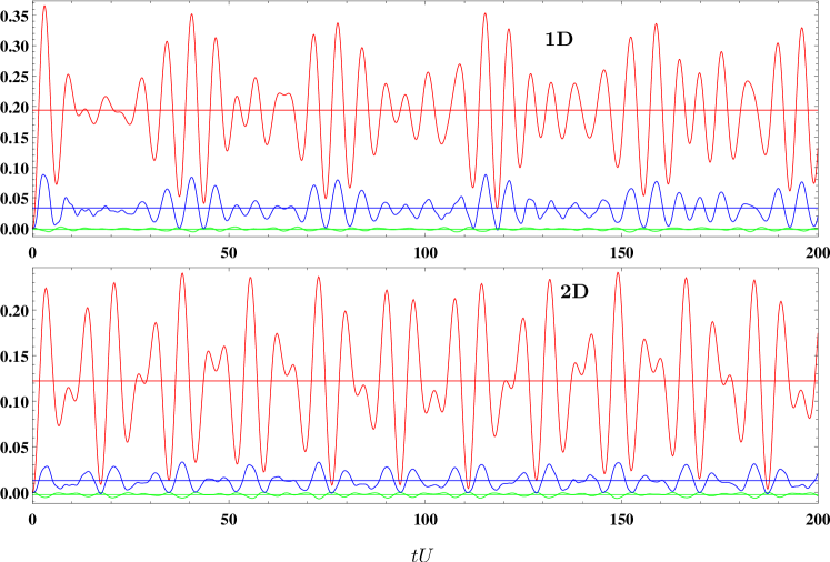
Figure 1: Two-point and three-point correlations. Correlation functions $\langle\hat{b}_{1}^{\dagger}\hat{b}_{2}\rangle$ (red), $\langle\hat{b}_{1}(\hat{b}_{2}^{\dagger})^{2}\hat{b}_{3}\rangle$ (blue), $\langle\hat{n}_{1}\hat{b}_{2}^{\dagger}\hat{b}_{3}\rangle^{\rm corr}$ (green) after quench $J/U=0\to 0.1$ calculated by exact diagonalization for one-dimensional lattice of $11$ sites (1D) and for two-dimensional lattice of $3\times 3$ sites (2D). Straight horizontal lines show the values averaged over an infinite evolution time.

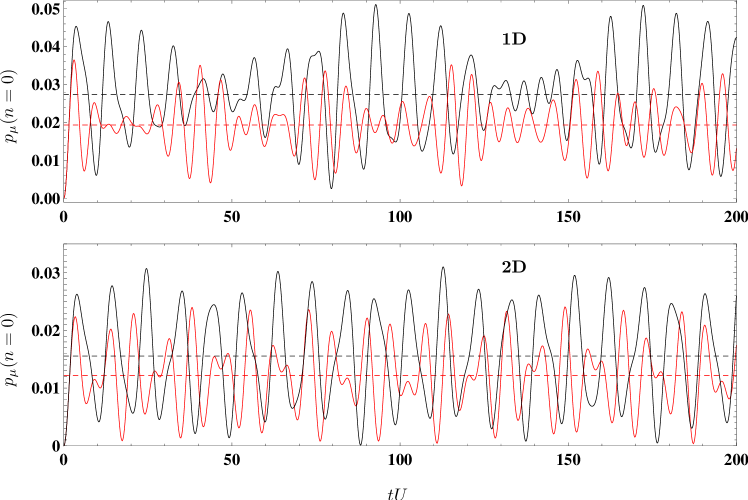
Figure 2: Approximate analytical solutions. Probability to have no particles on a lattice site in one-dimensional lattice of $11$ sites (1D) and for two-dimensional lattice of $3\times 3$ sites (2D). Red lines – exact diagonalization, black lines – Eq. (10). Dashed horizontal lines show the values averaged over an infinite evolution time.

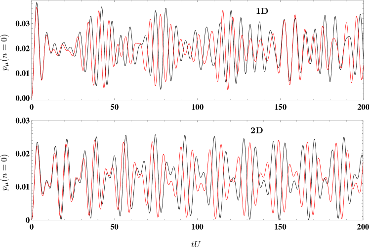
Figure 3: Numerical solutions for small lattices. Probability to have no particles on a lattice site in one-dimensional lattice of $11$ sites (1D) and for two-dimensional lattice of $3\times 3$ sites (2D). Red lines – exact diagonalization (the same as in Fig. 2), black lines – numerical solution of Eqs. (6), (8).

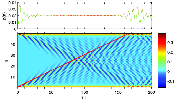
Figure 4: Numerical solutions for large lattice in 1D. Calculations for $50$ sites. Upper panel: Probabilities to have zero (red) and two (green) particles on a lattice site. Lower panel: $\langle\hat{b}_{\mu}^{\dagger}\hat{b}_{\mu+s}\rangle$, $s=1,\dots,49$. Red line $s=v_{\rm max}t$, $v_{max}=3J$.

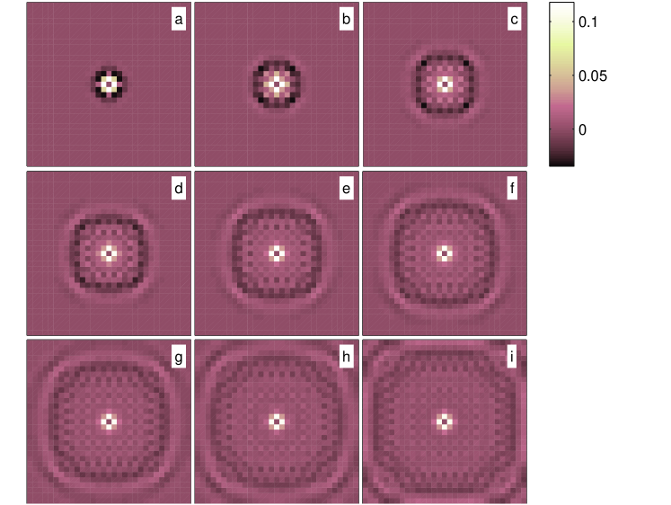
Figure 5: Anisotropic propagation of correlations in 2D. Calculations for $30\times 30$ sites. Coordinate dependences of the correlation function $\langle\hat{b}_{\mu_{1}}^{\dagger}\hat{b}_{\mu_{2}}\rangle$ at different times after quench: $tU=10$ (a), $20$ (b), $30$ (c), $40$ (d), $50$ (e), $60$ (f), $70$ (g), $80$ (h), $90$ (i).

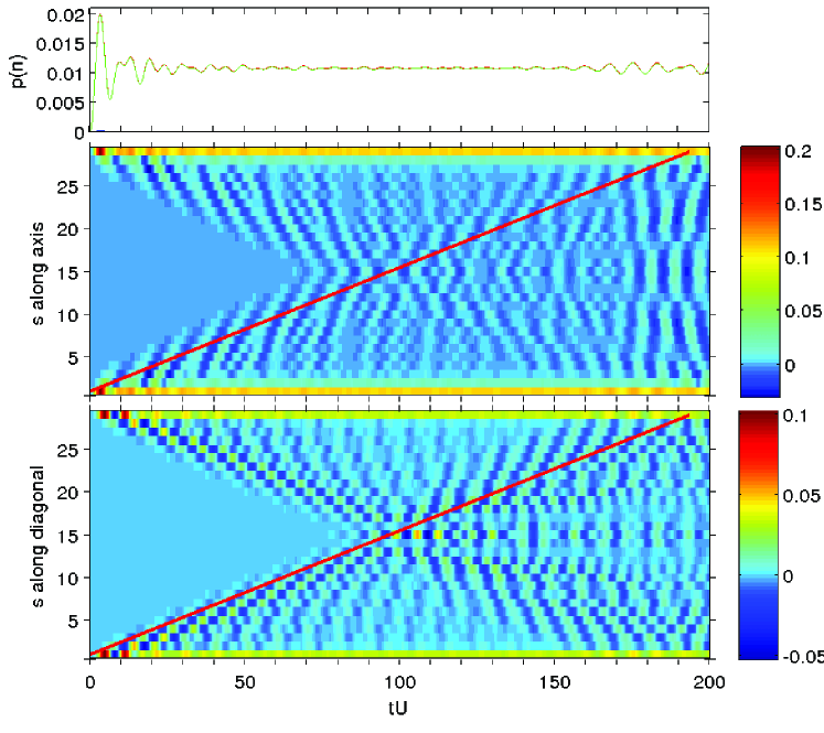
Figure 6: Numerical solutions for large lattice in 2D. Calculations for $30\times 30$ sites. Upper panel: Probabilities to have zero (red) and two (green) particles on a lattice site. Middle panel: $\langle\hat{b}_{\mu}^{\dagger}\hat{b}_{\mu+{\bf e}_{1}s}\rangle$, $s=1,\dots,29$. Red line $s=v_{\rm max}t$, $v_{\rm max}=3J$. Lower panel: $\langle\hat{b}_{\mu}^{\dagger}\hat{b}_{\mu+({\bf e}_{1}+{\bf e}_{2})s}\rangle$, $s=1,\dots,29$. Red line $s=\sqrt{2}\,v_{\rm max}t$, $v_{\rm max}=3J/\sqrt{2}$. ${\bf e}_{1}$ and ${\bf e}_{2}$ are unit vectors along the lattice axes.

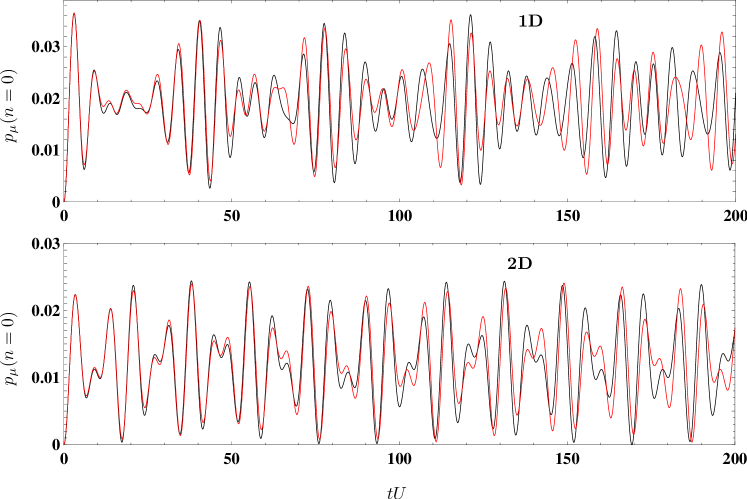
Figure 7: Numerical solutions for small lattices: three-point correlations. Probability to have no particles on a lattice site in one-dimensional lattice of $11$ sites (1D) and for two-dimensional lattice of $3\times 3$ sites (2D). Red lines – exact diagonalization (the same as in Fig. 2), black lines – numerical solution of the equations of motion for the reduced density matrices including three-point correlations.

Additional Files

Additional file 1 — fig1.eps

Additional file 2 — fig2.eps

Additional file 3 — fig3.eps

Additional file 4 — fig4.eps

Additional file 5 — fig5.eps

Additional file 6 — fig6.eps

Additional file 7 — fig7.eps

References

- [1]
- [2] Vidal, G.: Efficient simulation of one-dimensional quantum many-body systems. Phys Rev Lett 93, 040502 (2004)
- [3] Verstraete, F., Porras, D., Cirac, J.I.: Density matrix renormalization group and periodic boundary conditions: A quantum information perspective. Phys Rev Lett 93, 227205 (2004)
- [4] Cirac, J.I., Verstraete, F.: Renormalization and tensor product states in spin chains and lattices. J Phys A: Mathematical and Theoretical 42, 504004 (2009)
- [5] Schollwöck, U.: The density-matrix renormalization group in the age of matrix product states. Annals of Physics 326, 96–192 (2011)
- [6] Calabrese, P., Cardy, J.: Time dependence of correlation functions following a quantum quench. Phys Rev Lett 96, 136801 (2006)
- [7] Calabrese, P., Cardy, J.: Quantum quenches in extended systems. J Stat Mech: Theory and Experiment (2007) P06008
- [8] Kollath, C., Läuchli, A.M., Altman, E.: Quench dynamics and nonequilibrium phase diagram of the Bose-Hubbard model. Phys Rev Lett 98, 180601 (2007)
- [9] Rigol, M., Dunjko, V., Yurovsky, V., Olshanii, M.: Relaxation in a completely integrable many-body quantum system: an ab initio study of the dynamics of the highly excited states of 1D lattice hard-core bosons. Phys Rev Lett 98, 050405 (2007)
- [10] Rigol, M., Dunjko, V., Olshanii, M.: Thermalization and its mechanism for generic isolated quantum systems. Nature (London) 452, 854–858 (2008)
- [11] Eckstein, M., Hackl, A., Kehrein, S., Kollar, M., Moeckel, M., Werner, P., Wolf, F.A.: New theoretical approaches for correlated systems in nonequilibrium. Eur Phys J Spec Top 180, 217–235 (2009)
- [12] Moeckel, M., Kehrein, S.: Real-time evolution for weak interaction quenches in quantum systems. Ann Phys (NY) 324, 2146–2178 (2009)
- [13] Cazalilla, M.A., Rigol, M.: Focus on dynamics and thermalization in isolated quantum many-body systems. New J Phys 12, 055006 (2010)
- [14] Polkovnikov, A., Sengupta, K., Silva, A., Vengalattore, M.: Nonequilibrium dynamics of closed interacting quantum systems. Rev Mod Phys 83, 863–883 (2011)
- [15] Rigol, M.: Dynamics and thermalization in correlated one-dimensional lattice systems In: Proukakis, N.P., Gardiner, S.A., Davis, M.J., Szymanska, M.H. (eds.) Quantum Gases: Finite Temperature and Non-Equilibrium Dynamics, pp. –. Imperial College Press, London (2013). Cold Atoms Series vol 1
- [16] Rigol, M.: Quantum quenches in the thermodynamic limit. Phys Rev Lett 112, 170601 (2014)
- [17] Cramer, M., Flesch, A., McCulloch, I.P., Schollwöck, U., Eisert, J.: Exploring local quantum many-body relaxation by atoms in optical superlattices. Phys Rev Lett 101, 063001 (2008)
- [18] Flesch, A., Cramer, M., McCulloch, I.P., Schollwöck, U., Eisert, J.: . Phys Rev A 78, 033608 (2008)
- [19] Läuchli, A.M., Kollath, C.: Spreading of correlations and entanglement after a quench in the one-dimensional Bose–Hubbard model. J Stat Mech: Theory and Experiment (2008) P05018
- [20] Bernier, J-S., Poletti, D., Barmettler, P., Roux, G., Kollath, C.: Slow quench dynamics of Mott-insulating regions in a trapped Bose gas. Phys Rev A 85, 033641 (2012)
- [21] Barmettler, P., Poletti, D., Cheneau, M., Kollath, C.: Propagation front of correlations in an interacting Bose gas. Phys Rev A 85, 053625 (2012)
- [22] Natu, S.S., Mueller, E.J.: Dynamics of correlations in a dilute Bose gas following an interaction quench. Phys Rev A 87, 053607 (2013)
- [23] Natu, S.S., Mueller, E.J.: Dynamics of correlations in shallow optical lattices. Phys Rev A 87, 063616 (2013)
- [24] Deuar, P., Stóbinska, M.: Correlation waves after quantum quenches in one- to three-dimensional BECs. arXiv:1310.1301
- [25] Carleo, G., Becca, F., Sanchez-Palencia, L., Sorella, S., Fabrizio, M.: Light-cone effect and supersonic correlations in one- and two-dimensional bosonic superfluids. Phys Rev A 89, 031602(R) (2014)
- [26] Bonnes, L., Essler, F.H.L., Läuchli, A.M.: ”Light-cone” dynamics after quantum quenches in spin chains. arXiv:1404.4062
- [27] Bernier, J.-S., Citro, R., Kollath, C., Orignac, E.: Correlation dynamics during a slow interaction quench in a one-dimensional Bose gas. Phys Rev Lett 112, 065301 (2014)
- [28] Chen, D., White, M., Borries, C., DeMarco, B.: Quantum quench of an atomic Mott insulator. Phys Rev Lett 106, 235304 (2011)
- [29] Cheneau, M., Barmettler, P., Poletti, D., Endres, M., Schauß, P., Fukuhara, T., Gross, C., Bloch, I., Kollath, C., Kuhr, S.: Light-cone-like spreading of correlations in a quantum many-body system. Nature (London) 481, 484–487 (2012)
- [30] Trotzky, S., Chen, Y-A., Flesch, A., McCulloch, I.P., Schollwöck, U., Eisert, J., Bloch, I.: Probing the relaxation towards equilibrium in an isolated strongly correlated one-dimensional Bose gas. Nature Physics 8, 325–330 (2012)
- [31] Queisser, F., Krutitsky, K.V., Navez, P., Schützhold, R.: Equilibration and prethermalization in the Bose-Hubbard and Fermi-Hubbard models. Phys Rev A 89, 033616 (2014)
- [32] Navez, P., Schützhold, R.: Emergence of coherence in the Mott-superfluid quench of the Bose-Hubbard model. Phys Rev A 82, 063603 (2010)
- [33] Queisser, F., Navez, P., Schützhold, R.: Sauter-Schwinger like tunneling in tilted Bose-Hubbard lattices in the Mott phase. Phys Rev A 85, 033625 (2012)
- [34] Queisser, F., Navez, P., Schützhold, R.: Universal frozen spectra after time-dependent symmetry restoring phase transitions. J Phys: Cond Mat 25, 404215 (2013)
- [35] Navez, P., Queisser, F., Schützhold, R.: Quasi-particle approach for lattice Hamiltonians with large coordination numbers. J Phys A: Math Theor 47, 225004 (2014)
- [36] Berges, J., Borsányi, S., Wetterich, C.: Prethermalization. Phys Rev Lett 93, 142002 (2004)
- [37] Kollar, M., Wolf, F.A., Eckstein, M.: Generalized Gibbs ensemble prediction of prethermalization plateaus and their relation to nonthermal steady states in integrable systems. Phys Rev B 84, 054304 (2011)
- [38] Kitagawa, T., Imambekov, A., Schmiedmayer, J., Demler, E.: The dynamics and prethermalization of one-dimensional quantum systems probed through the full distributions of quantum noise. New J Phys 13, 073018 (2011)
- [39] Birrell, N.D., Davies, P.C.W.: Quantum Fields in Curved Space. Cambridge University Press, Cambridge (1984)
- [40] Schützhold, R., Unruh, W.G.: Cosmological particle creation in the lab? In: Faccio, D., Belgiorno, F., Cacciatori, S., Gorini, V., Liberati, S., Moschella, U. (eds.) Analogue Gravity Phenomenology: Analogue Spacetimes and Horizons, from Theory to Experiment, pp. 51–61. Springer, New York (2013). Lecture Notes in Physics, vol 870