Default Probability Estimation via Pair Copula Constructions

Abstract

In this paper we present a novel approach for firm default probability estimation. The methodology is based on multivariate contingent claim analysis and pair copula constructions. For each considered firm, balance sheet data are used to assess the asset value, and to compute its default probability. The asset pricing function is expressed via a pair copula construction, and it is approximated via Monte Carlo simulations. The methodology is illustrated through an application to the analysis of both operative and defaulted firms.

1 Introduction

Default risk is defined as the risk of a loss when a debtor (in our case a firm) does not fulfil its commitments in a financial contract, and a default event takes place. The probability of default (PD) is the probability that a default happens.

Following the growing financial uncertainty, there has been intensive research by institutions, regulators and academics to develop models for firm evaluation and PD estimation. The existing methodologies differ on the available information and data used for assessing the firm value. They can be broadly classified in models based on market data and on accounting data.

Within the market data based models, the most popular are structural models; see Merton (1970, 1974, 1977) and their extensions; for recent and complete reviews, see e.g. Ji (2010), Laajimi (2012), or Sundaresan (2013). The asset value is considered to be exogenous and it is treated as the underlying asset in a contingent claim framework. A common assumption is that the asset value follows a geometric Brownian motion, and its drift and volatility coefficients do not depend on the capital structure of the firm. Black and Scholes’ formula is applied to compute the asset price, and consequently the PD can be easily estimated, see Black and Scholes (1973).

The second class of models use accounting data and financial ratios to evaluate the firm value, and its PD. They origin from the works of Beaver (1968) and Altman (1968) who developed univariate and multivariate models, based on linear discriminant analysis, to predict the default of specific firms by using a set of financial ratios. Another commonly used default prediction model is based on logistic regression, as proposed by Ohlson (1980).

The previous models have been analysed both in a classical and in a Bayesian framework. For some recent works in the classical framework, see e.g. Bharath and Shumway (2008), De Giuli et al. (2008), Kreinin and Nagi (2008), Su and Huang (2010), Altman et al. (2011), Bo et al. (2011, 2013), Bhimani et al. (2014), Leow and Crook (2015), Tobback et al. (2014), and references therein. For the Bayesian analysis see e.g. Kiefer (2009, 2010, 2011), Park et al. (2010), Tasche (2011), Kazemi and Mosleh (2012), Orth (2013), Liu et al. (2015), and references therein.

A popular and efficient tool in risk management is the copula function, introduced by Sklar (1959). The advantage of copulas is the ability to obtain the joint multivariate distribution embedding the variable’s dependence structure. Unfortunately, while there is a wide range of possible alternative copula functions for the bivariate case, in the multivariate setting the use of families different from Normal and Student’s t is rather scarce, due to computational and theoretical limitations. For this reason Joe (1996) introduced Pair Copula Constructions (PCCs) to represent complex structures of dependence among multivariate data. PCCs constitute a flexible and very appealing tool for financial analysis, see e.g. Vaz de Melo Mendes et al. (2010), Min and Czado (2010), Allen et al. (2013), Dißmann et al. (2013), Bernard and Czado (2013), and reference therein. A collection of potentially different bivariate copulas is used to construct the joint distribution of interest via PCCs, allowing to represent different types and strengths of dependence in an easy way.

In this paper we propose a novel approach for PD estimation, that combines features of both structural and accounting based models. We consider a contingent claim model based on balance sheet data, where the dynamic of the equity is described via a PCC and calculated using Monte Carlo simulations. We apply Bayesian parametric mixture models in the new context of vine marginal modelling, for balance sheet data of defaulted and non-defaulted firms. The PD is obtained in a fairly straightforward way from the equity distribution.

The outline of the paper is the following. In Section 2 we briefly present copula models and PCCs. In Section 3 we introduce a novel balance sheet multivariate contingent claim model for PD estimation based on PCCs. In Section 4 the model estimation methodology is presented. Section 5 describes the application of the proposed methodology to the PD estimation of defaulted and operative companies. Finally, concluding remarks are given in Section 6.

2 Background and Preliminaries

2.1 Copula Function

Copulas are very popular and appealing statistical tools, that allow us to describe complex multivariate patterns of dependence binding together the marginal distributions. They are applicable to a wide variety of fields, such as economics, finance and marketing; for a review see e.g. Jaworski (2010).

A copula is a multivariate distribution function with uniform marginals on the interval $[0,1]$. Once applied to the univariate marginals, it returns the multivariate joint distribution, enclosing all the information about the dependence structure of the variables. Thus, the use of copulas allows us to split the distribution of a random vector into its individual marginal components, and the dependence structure is modelled through the copula function without losing information; for more details see e.g. Joe (1997) and Nelsen (1999).

Sklar’s theorem is the most important result in copula theory. It states that, given a vector of random variables $\textbf{X}=(X_{1},\ldots,X_{d})$, with $d$-dimensional joint cumulative distribution function $F(x_{1},\ldots,x_{d})$ and marginal cumulative distributions $F_{m}(x_{m})$ with $m=1,\ldots,d$, there exist a $d$-dimensional copula $C$ such that

$$F(x_{1},\ldots,x_{d})=C(F_{1}(x_{1}),\ldots,F_{d}(x_{d});\boldsymbol{\theta}),$$ (1)

where $\boldsymbol{\theta}$ denotes the set of parameters of the copula. To simplify the notation, in the remainder of the paper, we set

$$C(F_{1}(x_{1}),\ldots,F_{d}(x_{d}))=C(F_{1}(x_{1}),\ldots,F_{d}(x_{d});\boldsymbol{\theta}).$$

For an absolutely continuous joint distribution $F$ with strictly increasing continuous marginal distribution functions, the $d$-dimensional copula is uniquely defined. Conversely, according to Nelsen’s corollary, the inversion method allows us to express the copula in the following way

$$C(u_{1},\ldots,u_{d})=F(F_{1}^{-1}(u_{1}),\ldots,F_{d}^{-1}(u_{d})),$$

where $F_{1}^{-1},\ldots,F_{d}^{-1}$ are the generalised inverse functions of the marginals.

The joint density function is

$$f(x_{1},\ldots,x_{d})=c(F_{1}(x_{1}),\ldots,F_{d}(x_{d}))\cdot f_{1}(x_{1})\cdots f_{d}(x_{d}),$$

where $c(F_{1}(x_{1}),\ldots,F_{d}(x_{d}))$ is the $d$-variate copula density, provided its existence.

In this paper, we fit the data into a given model following a parametric approach. Nonparametric methods for copula density estimation also exist, see e.g. Sancetta and Satchell (2004), Shen et al. (2008) and Kauermann et al. (2013).

The existing literature on copulas mainly focuses on the bivariate case. In the multivariate case, Normal and Student’s t copula are the most popular, while the use of other multidimensional copulas is rather limited, due to the complexity of their construction, see e.g. Aas and Berg (2009). However, Normal and Student’s t copula are often not flexible enough to represent the dependence structure of the data. Hence, multivariate extensions of Archimedean copulas were proposed in the form of partially nested Archimedean copulas by Joe (1997) and Whelan (2004); hierarchical Archimedean copulas by Savu and Trede (2006); and multiplicative Archimedean copulas by Morillas (2005) and Liebscher (2006). Nevertheless, these multivariate extensions imply additional restrictions on the parameters that limit their flexibility. A possible solution to this problem is provided by PCCs, that will be described in the following section.

2.2 Pair Copula Constructions

We now briefly introduce PCCs, the related notation and terminology; for more details see e.g. Czado (2010). PCCs were originally proposed by Joe (1996), and later discussed in detail by Bedford and Cooke (2001, 2002), Kurowicka and Cooke (2006) and Aas et al. (2009). For some recent works in a parametric and nonparametric framework see e.g. Min and Czado (2010), Bauer et al. (2012), Nikoloulopoulos et al. (2012), Weiß  and Scheffer (2012), Haff and Segers (2015).

A PCC represents the complex pattern of dependence of multivariate data via a cascade of bivariate copulas, and permits to construct flexible high-dimensional copulas by using only bivariate copulas as building blocks, see Aas et al. (2009). Therefore, the joint distribution is obtained on the basis of bivariate pair copulas, that may be conditional on a specific set of variables, allowing to model the dependence among the marginals.

In order to obtain a PCC we proceed as follows. First of all we factorise the joint distribution $f(x_{1},\ldots,x_{d})$ of the random vector $\textbf{X}=(X_{1},\ldots,X_{d})$ as a product of conditional densities

$$f(x_{1},\ldots,x_{d})=f_{d}(x_{d})\times f_{d-1|d}(x_{d-1}|x_{d})\times\ldots\times f_{1|2\cdots d}(x_{1}|x_{2},\ldots,x_{d}).$$ (2)

The factorisation in (2) is unique up to re-labeling of the variables, and it can be reexpressed in terms of a product of bivariate copulas. By Sklar’s theorem the joint distribution of the subvector $(X_{d},X_{d-1})$ can be expressed in terms of a copula density

$$f(x_{d-1},x_{d})=c_{d-1,d}(F_{d-1}(x_{d-1}),F_{d}(x_{d}))\times f_{d-1}(x_{d-1})\times f_{d}(x_{d}),$$

where $c_{d-1,d}(\cdot,\cdot)$ is an arbitrary bivariate copula (pair copula) density. Hence, the conditional density of $X_{d-1}|X_{d}$ can be easily rewritten as

$$f_{d-1|d}(x_{d-1}|x_{d})=c_{d-1,d}(F_{d-1}(x_{d-1}),F_{d}(x_{d}))\times f_{d-1}(x_{d-1}).$$ (3)

Through a straightforward generalisation of equation (3), each term in (2) can be decomposed into the appropriate pair copula times a conditional marginal density. More precisely, for a generic element $X_{\jmath}$ of the vector X we obtain

$$f_{x_{\jmath}|\textbf{v}}(x_{\jmath}|\textbf{v})=c_{x_{\jmath},v_{\ell}|\textbf{v}_{-\ell}}(F_{x_{\jmath}|\textbf{v}_{-\ell}}(x_{\jmath}|\textbf{v}_{-\ell}),F_{v_{\ell}|\textbf{v}_{-\ell}}(v_{\ell}|\textbf{v}_{-\ell}))\times f_{x_{\jmath}|\textbf{v}_{-\ell}}(x_{\jmath}|\textbf{v}_{-\ell}),$$ (4)

where v is the conditioning vector, $v_{\ell}$ is a generic component of v, $\textbf{v}_{-\ell}$ is the vector v without the component $v_{\ell}$, $F_{x_{\jmath}|\textbf{v}_{-\ell}}(\cdot|\cdot)$ is the conditional distribution of $x_{\jmath}$ given $\textbf{v}_{-\ell}$, and $c_{x_{\jmath},v_{\ell}|\textbf{v}_{-\ell}}(\cdot,\cdot)$ is the conditional pair copula density. The $d$-dimensional joint multivariate distribution function can hence be expressed as a product of bivariate copulas and marginal distributions by recursively plugging equation (4) in equation (2). Such decomposition is named PCC, as introduced by Joe (1996).

Note that the PCC decomposition in (4) is based on the simplifying assumption that the conditional copulas depend on the conditioning variables only indirectly through the conditional distribution functions that constitute their arguments. However, as demonstrated by Haff et al. (2010), the simplified PCC is a good approximation, even when the simplifying assumption is far from being fulfilled by the actual model.

The PCC is order dependent. A different choice of the variable order leads to a different PCC and to a different factorisation of the joint multivariate distribution.

Furthermore, given a specific factorisation there are still many different parameterisations. For high-dimensional distributions, the number of possible PCCs is very high, see Czado (2010) and Morales-Napoles (2011). Hence a suitable representation of all of them is necessary. For this reason, Bedford and Cooke (2001, 2002) introduced Regular vines (R-vines) as a pictorial representation of PCCs.

R-vines are a particular type of graphical models, that use a nested set of trees to represent the decomposition of the joint distribution into its bivariate components, incorporating the dependence structure of the variables of interest. Two special cases of R-vines are Canonical vines (C-vines) and Drawable vines (D-vines), see Kurowicka and Cooke (2006). Here we consider a four dimensional problem, for which R-vines are either C-vines or D-vines. We concentrate on D-vines because, differently from C-vine, they do not assume the existence of a particular node dominating the dependencies.

A vine ${\cal V}(d)$ on $d$ variables is a nested set of trees $T_{1},\ldots,T_{d-1}$. The edges of tree $T_{\tau}$ are the nodes of tree $T_{\tau+1}$, $\tau=1,\ldots,d-1$. In a R-vine, if two edges of tree $T_{\tau}$ share a common node, they are represented in tree $T_{\tau+1}$ by nodes joined by an edge. A D-vine is a R-vine where all nodes do not have degree higher than $2$, that is each node is connected to no more than two other nodes.

In a D-vine, each node corresponds to a variable or a set of variables. A pair-copula density is associated to any edge, with the edge label indicating the subscript of the pair-copula density. An example of a $4$-dimensional D-vine is provided by Figure 1. The first tree is constructed ordering the variables according to their pairwise dependence, where the first two nodes correspond to the variables with the strongest association, and so on; the dependencies between nodes $\{1\}$ and $\{2\}$, between $\{2\}$ and $\{3\}$, and between $\{3\}$ and $\{4\}$ are modelled using bivariate copula distributions. In the second tree, the conditional dependencies between nodes $\{1,2\}$ and $\{2,3\}$, and between $\{2,3\}$ and $\{3,4\}$ are modelled via pair copula densities. In the third tree, the conditional dependence between nodes $\{1,3|2\}$ and $\{2,4|3\}$ is modelled via a pair copula density.

Figure 1: 4-dimensional D-vine graphical representation

Using the D-vine representation, the joint density can be decomposed in terms of conditional copula densities (identified by the labels of the edges in the considered trees) times the marginal densities of the examined variables. The joint density for the D-vine represented in Figure 1 is given by

$$f(x_{1},\ldots,x_{4})=\prod_{\tau=1}^{4}f_{\tau}(x_{\tau})\times c_{12}\times c_{23}\times c_{34}\times c_{13|2}\times c_{24|3}\times c_{14|23},$$

where $c_{ab}=c_{ab}(F(x_{a}),F(x_{b}))$.

More generally, the density of a D-vine of dimension $d$ takes the form

$$f(x_{1},\ldots,x_{d}) = \prod_{\tau=1}^{d}f_{\tau}(x_{\tau})\times$$

$$\prod_{j=1}^{d-1}\prod_{i=1}^{d-j}c_{i,i+j|i+1,\ldots,i+j-1}(F(x_{i}|x_{i+1},\ldots,x_{i+j-1}),F(x_{i+j}|x_{i+1},\ldots,x_{i+j-1}))$$

which is the product of $d$ marginal densities $f_{\tau}$ and $d(d-1)/2$ bivariate copulas $c_{i,i+j|i+1,\ldots,i+j-1}(\cdot,\cdot)$ evaluated at the conditional distribution functions $F(\cdot|\cdot)$.

If marginal or conditional independence between pairs of variables holds, the corresponding pair copulas are equal to one and hence the PCC and joint density simplify accordingly. The case of independence is depicted in the corresponding vine by missing edges between nodes, obtaining a forest vine, as shown in Figure 2. Here, conditional independence between variables $2$ and $4$ given $3$ is represented by the missing edge $\{2,4|3\}$, which reduces the number of levels of the PCC.

Figure 2: Forest vine

3 A Balance Sheet Multivariate Contingent Claim Model

In this paper we propose a novel contingent claim model for PD estimation via PCCs on balance sheet data, that refines and improves Merton’s analysis. Our approach allows us to evaluate, at any time $t$, the company ability to service its debts, and consequently to efficiently predict its PD in a flexible way. In the following Section we describe the main characteristics of Merton’s model, and introduce our approach.

3.1 Merton’s Model

According to Merton (1970, 1974, 1977), the evaluation of the firm total assets $A_{t}$ is based on the structural variables equity $E_{t}$ and bond $B_{t}$,

$$A_{t}=E_{t}+B_{t}.$$

A very common assumption is that the value $A_{t}$ of the firm follows a geometric Brownian motion

$$\mathrm{d}A_{t}=\mu_{A}A_{t}\,\mathrm{d}t+\sigma_{A}A_{t}\,\mathrm{d}W_{t},$$

where $\mu_{A}$ is the instantaneous expected return of the asset, $\sigma_{A}$ is the volatility, and $W_{t}$ is a Wiener process. Under the assumptions of market efficiency, no arbitrage opportunity and continuous hedging, the market value of equity satisfies

$$E_{t}=A_{t}N(d_{1})-e^{-rT}DN(d_{2}),$$ (5)

where $r$ is the risk free interest rate, $N(\cdot)$ is the cumulative standard Normal distribution function, $D$ is the face value of bond at maturity $T$, $d_{1}$ is given by

$$d_{1}=\frac{\log(A_{t}/D)+(\mu_{A}+0.5\sigma^{2}_{A})T}{\sigma_{A}\sqrt{T}}$$

and $d_{2}=d_{1}-\sigma_{A}\sqrt{T}$. Furthermore, the volatility of the equity is

$$\sigma_{E}=\frac{A_{t}}{E_{t}}N(d_{1})\sigma_{A}.$$ (6)

The asset value and its volatility, $A_{t}$ and $\sigma_{A}$ respectively, cannot be directly observed; however they may be obtained solving equations (5) and (6), see e.g. Ronn and Verma (1986). Consequently we can easily obtain $d_{2}$, and $PD=Pr[A_{T}\leq B_{T}]=N(-d_{2})$.

This model has some drawbacks. Its structure implies that equity and asset values are non negative in trading markets, whereas negative asset and equity are possible in accounting, see e.g. Peterkort and Nielsen (2005). Furthermore, only part of the total debt is traded and observable at specific accounting periods. Finally, Merton’s model might underestimate failure probability, see e.g. De Giuli et al. (2008) and Su and Huang (2010). One possible solution to these issues is proposed in the following Section.

3.2 The Default Probability Model

In order to solve the asset observability issue, we model the firm value via a contingent claim on the underlying securities (equity and debt). We use balance sheet data as a proxy of market data, and we apply PCCs to model the equity dynamic. For a recent work on PCCs in contingent claim analysis see Bernard and Czado (2013).

The value of a contingent claim at maturity $T$ can be written in a general form as $G(S_{1}(T),S_{2}(T)),$ where $G(\cdot)$ is the pay-off function, and $S_{1}(T)$ and $S_{2}(T)$ are the underlying securities at maturity $T$. In this framework the final value of the firm is given by $\textsf{A}_{T}=G(\textsf{E}_{T},\textsf{B}_{T};T)$ where $\textsf{E}_{T}$ and $\textsf{B}_{T}$ denote, respectively, equity and debt at maturity $T$. In a similar way we can express the equity as $\textsf{E}_{T}=G_{1}(\textsf{A}_{T},\textsf{B}_{T};T)=(\textsf{A}_{T}-\textsf{B}_{T})$ where $G_{1}(\cdot)$ is the pay-off function with density $g_{1}(\cdot)$. The equity value at time $t$ is computed as

$$\textsf{E}_{t}=G_{1}(\textsf{A}_{t},\textsf{B}_{t};t)=P(t,T)\int_{0}^{\infty}\int_{0}^{\infty}G_{1}(\textsf{A}_{T},\textsf{B}_{T};T)g_{1}(\textsf{A}_{T},\textsf{B}_{T})d\textsf{A}_{T}d\textsf{B}_{T},$$ (7)

where $P(t,T)$ is the risk free discount factor.

The firm value and its return volatility are not directly observable, hence we use balance sheet data, denoted by $A_{T}$ (asset) and $B_{T}$ (liability), as reliable proxy of the market data, see e.g. Eberhart (2005). Assets represent what a firm owns, whereas liabilities are debts arising from business operations. We decompose $A_{T}$ and $B_{T}$ in current ($C_{T}$) and long term components ($L_{T}$) on the basis of the considered time period; that is $A_{T}=A_{C_{T}}+A_{L_{T}}$ and $B_{T}=B_{C_{T}}+B_{L_{T}}$. Current assets will be converted into cash within one year, whereas long term assets will be converted after more than one year. In a similar way, the firm expects to pay off current liabilities within one year; whereas, the firm expects to settle long term liabilities after one year. Comparing current/long term assets with current/long term liabilities we can obtain a quick gauge of the financial status of the firm. In fact, standard accounting ratios commonly used to investigate the financial strength and efficiency of a firm are based on these quantities.

Equation (7) can be rewritten in terms of balance sheet data as follows

$$E_{t} = G_{2}(A_{C_{t}},A_{L_{t}},B_{C_{t}},B_{L_{t}};t)=$$

$$= \!P(t,T)\int_{0}^{\infty}\!\int_{0}^{\infty}\!\int_{0}^{\infty}\!\int_{0}^{\infty}\!G_{2}(A_{C_{T}},A_{L_{T}},B_{C_{T}},B_{L_{T}};T)\times$$

$$\times g_{2}(A_{C_{T}},A_{L_{T}},B_{C_{T}},B_{L_{T}})dA_{C_{T}}dA_{L_{T}}dB_{C_{T}}dB_{L_{T}},$$

where $G_{2}(\cdot)$ and $g_{2}(\cdot)$ are respectively the pay-off function and its density for the decomposed data.

By using Sklar’s theorem the 4-dimensional density function $g_{2}(A_{C_{T}},A_{L_{T}},B_{C_{T}},B_{L_{T}})$ can be expressed via a copula, and the equity becomes

$$E_{t} = P(t,T)\int_{0}^{\infty}\int_{0}^{\infty}\int_{0}^{\infty}\int_{0}^{\infty}G_{2}(A_{C_{T}},A_{L_{T}},B_{C_{T}},B_{L_{T}};T)\times$$ (8)

$$\times c(F_{A_{C}},F_{A_{L}},F_{B_{C}},F_{B_{L}})f_{A_{C}}f_{A_{L}}f_{B_{C}}f_{B_{L}}dA_{C_{T}}dA_{L_{T}}dB_{C_{T}}dB_{L_{T}},$$

where $c(\cdot)$ denotes the $4$-dimensional copula density function, $F_{A_{C}}$, $F_{A_{L}}$, $F_{B_{C}}$, $F_{B_{L}}$ are the marginal cumulative distribution functions, and $f_{A_{C}},f_{A_{L}},f_{B_{C}},f_{B_{L}}$ are the marginal probability density functions.

In order to improve the flexibility of the model, allowing the dependence pattern of each pair of variables to be represented by a different copula, we reexpress the previous equation via PPCs. The $4$-dimensional copula density function $c(F_{A_{C}},F_{A_{L}},F_{B_{C}},F_{B_{L}})$ is decomposed in terms of a sequence of bivariate copulas, not necessary belonging to the same family of distributions, via a D-vine decomposition. The specific decomposition depends on the particular data structure under examination; see Section 5 for the details.

Simulating from the D-vine decomposition we can approximate the equity function in equation (8) via Monte Carlo method as follows

$$\tilde{E}_{t}=P(t,T)\frac{1}{N}\sum_{k=1}^{N}G_{2}(\tilde{A}_{C_{Tk}},\tilde{A}_{L_{Tk}},\tilde{B}_{C_{Tk}},\tilde{B}_{L_{Tk}};T),$$

where $N$ is the number of simulations, $\tilde{E}_{t},\tilde{A}_{C_{Tk}},\tilde{A}_{L_{Tk}},\tilde{B}_{C_{Tk}}$ and $\tilde{B}_{L_{Tk}}$ are the simulated values of equity, current and long term assets and liabilities. We then estimate the PD at time $t$ as $(PD)_{t}=Pr(\tilde{E}_{t}\leq 0)$. More details about simulating from a D-vine can be found in Aas et al. (2009).

4 Model Estimation

The dynamic of the equity value in equation (8) depends on the parameters of the copula and those of the marginal distributions. We denote with $\boldsymbol{\theta}$ the parameter vector of the copula function $c(F_{A_{C}},F_{A_{L}},F_{B_{C}},F_{B_{L}})$, and with $\boldsymbol{\delta_{m}}$ the parameter vector of the marginal distribution $m$, $m\in\{A_{C},A_{L},B_{C},B_{L}\}$. The vector $\Delta=(\boldsymbol{\delta_{A_{C}}},\boldsymbol{\delta_{A_{L}}},\boldsymbol{\delta_{B_{C}}},\boldsymbol{\delta_{B_{L}}})$ contains the parameters of the marginals, and $\Psi=(\Delta,\boldsymbol{\theta})$ represents the full set of parameters associated to (8).

In order to estimate $\Psi$ we follow the Inference Functions for Margins (IFM) procedure proposed by Joe and Xu (1996). The IFM method estimates the marginal parameters $\Delta$ in a first step, and then estimates the copula parameters $\boldsymbol{\theta}$, given $\hat{\Delta}_{IFM}$, in a second step.

4.1 Marginal Parameter Estimation

In order to model the marginals we adopted a parametric approach based on a two-component Normal mixture. This approach was motivated by extensive tests and simulation studies, that are described in Section 5.1.

The use of mixture distributions to model multimodal phenomena is a popular technique, which has attracted the interest of several authors in the literature, see e.g. McLachlan and Peel (2000). Peel and McLachlan (2000) use the ECM algorithm to fit mixtures of Student’s t distributions to data containing groups of observations with heavy tails or atypical observations. Komarek and Lesaffre (2008) propose to model the random effects of generalised linear mixed models by a mixture of Gaussian distributions, estimating the parameters in a Bayesian context using MCMC techniques. Escobar and West (1995) use mixture of Dirichlet processes for density estimation. For a review of Bayesian nonparametric methods for density estimation see e.g. Müller et al. (2015). Benaglia et al. (2009) provide a set of R functions, based on EM algorithms, for analysing a variety of finite mixture models, such as mixtures of regressions, multinomial mixtures, nonparametric and semiparametric mixture models. Schellhase and Kauermann (2012) represent unknown densities, allowed to depend on covariates, by a mixture of basis densities, using penalised splines.

The current and long term assets and liabilities present bimodal distributions. This behaviour can find an explanation in the effect of the managerial actions and decisions performed to improve the status of the firm. These actions and decisions directly impact the dynamic of current and long term assets and liabilities, and this can intuitively explain the presence of two separated clusters of data.

Let $F(x_{m_{t}})$ be the cumulative distribution function of the marginal $m$ at time $t$. We estimate each marginal distribution $F(x_{m_{t}})$ via a two-component Normal mixture model, assuming different means but equal variances (location-shift model)

$$F(x_{m_{t}})=\sum_{p=1}^{2}\eta_{p}\Phi(x_{m_{t}}|\mu_{p},\sigma^{2}).$$ (9)

In (9) $\eta_{p}$ is the classification probability for component $p$ (with $\eta_{p}\geq 0$ and $\sum_{p=1}^{2}\eta_{p}=1$), and $\Phi(x_{m_{t}}|\mu_{p},\sigma^{2})$ is the Normal cumulative distribution function with mean $\mu_{p}$ and variance $\sigma^{2}$. The likelihood is given by

$$L(x_{m})=\prod_{t=1}^{\mathfrak{n}}\sum_{p=1}^{2}\eta_{p}\phi(x_{m_{t}}|\mu_{p},\sigma^{2}),$$

where $\mathfrak{n}$ is the number of balance sheet observations, and $\phi$ is the probability density function of the Normal distribution.

Although based on standard distributions, mixture models pose highly complex computational challenges. In particular, one major difficulty is parameters estimation. The literature about mixture models offers various solutions both in the classical and in the Bayesian framework. Considering the classical approach, the most popular method is the EM algorithm, which is a numerical optimisation procedure allowing to calculate the maximum likelihood estimator. However this algorithm may fail to converge to the mode of the likelihood, see e.g. Marin et al. (2005). The Bayesian approach constitutes a more flexible and computationally convenient solution to the estimation of mixture models, allowing complex structures to be decomposed into a set of simpler structures through the use of latent variables. Moreover, the Bayesian approach permits, via the use of prior distributions, to incorporate into the model available additional information coming from different data sources. Furthermore, differently from the classical approach, the Bayesian one provides reliable parameter estimates even for sample sizes of limited dimension.

For the previous reasons, we use the Bayesian approach to model the dynamic of current and long term asset and liability data. The posterior distribution of the $m$-th marginal is given by

$$\pi(\boldsymbol{\delta_{m}},\boldsymbol{\eta}|\boldsymbol{x})\propto\left(\prod_{t=1}^{\mathfrak{n}}\sum_{p=1}^{2}\eta_{p}\phi(x_{t}|\boldsymbol{\delta_{m}})\right)\times\pi(\boldsymbol{\delta_{m}},\boldsymbol{\eta}),$$

where $\boldsymbol{x}$ is the balance sheet data vector, $\pi(\boldsymbol{\delta_{m}},\boldsymbol{\eta})$ is the joint prior distribution of $\boldsymbol{\delta_{m}}$ and the vector of classification probabilities $\boldsymbol{\eta}$. The posterior $\pi(\boldsymbol{\delta_{m}},\boldsymbol{\eta}|\boldsymbol{x})$ is computationally intractable to work with; hence, the data augmentation MCMC algorithm is used to estimate the parameters of the mixture distributions, see Tanner and Wong (1987). The data augmentation algorithm introduces a vector of latent variables $\boldsymbol{z}=(z_{1},\ldots,z_{\mathfrak{n}})$, that represents the allocations associated to each observation $x_{t}$. Hence, the posterior density can be expressed as

$$\pi(\boldsymbol{\delta_{m}},\boldsymbol{\eta}|\boldsymbol{x})=\int_{Z}\pi(\boldsymbol{\delta_{m}},\boldsymbol{\eta}|\boldsymbol{z},\boldsymbol{x})\pi(\boldsymbol{z}|\boldsymbol{x})d\boldsymbol{z},$$

where $\pi(\boldsymbol{z}|\boldsymbol{x})$ denotes the predictive density of the latent data $\boldsymbol{z}$ given $\boldsymbol{x}$, with $\boldsymbol{z}=(z_{1},\ldots,z_{\mathfrak{n}})$, and $\pi(\boldsymbol{\delta_{m}},\boldsymbol{\eta}|\boldsymbol{z},\boldsymbol{x})$ is the conditional density of the parameters given the augmented data. Moreover, $\pi(\boldsymbol{\delta_{m}},\boldsymbol{\eta}|\boldsymbol{z},\boldsymbol{x})=\pi(\boldsymbol{\delta_{m}}|\boldsymbol{\eta},\boldsymbol{z},\boldsymbol{x})\pi(\boldsymbol{\eta}|\boldsymbol{z},\boldsymbol{x})$, and $\pi(\boldsymbol{\eta}|\boldsymbol{z},\boldsymbol{x})=\pi(\boldsymbol{\eta}|\boldsymbol{z})$, since the distribution is independent of $\boldsymbol{x}$. The data augmentation algorithm uses an iterative procedure simulating $\boldsymbol{z}$ first, then generating $\boldsymbol{\eta}$ from $\pi(\boldsymbol{\eta}|\boldsymbol{z})$ and finally generating $\boldsymbol{\delta_{m}}$ from $\pi(\boldsymbol{\delta_{m}}|\boldsymbol{\eta},\boldsymbol{z},\boldsymbol{x})$. The densities $\pi(\boldsymbol{\eta}|\boldsymbol{z})$ and $\pi(\boldsymbol{\delta_{m}}|\boldsymbol{\eta},\boldsymbol{z},\boldsymbol{x})$, are easier to sample than the original posterior.

Assuming independency between parameters a priori, we specify the following prior distributions

$$z_{t} \sim {Bernoulli}(\eta_{1})$$

$$(\eta_{1},\eta_{2}) \sim Dirichlet(\alpha_{1},\alpha_{2})$$

$$\mu_{p} \sim Normal(b_{p},B_{p})$$

$$\sigma^{2} \sim \Gamma^{-1}\left(\nu/2,\nu S/2\right),$$

where a convenient choice of hyperparameters $\alpha_{1},\alpha_{2},b_{p},B_{p},\nu,S$ leads us to vague prior distributions. A sensitivity analysis was carried out proposing different hyperparameter values; however, the high similarity of all results suggested that the model is insensitive to prior parameter choice.

We need to point out that the simulations were implemented using the software JAGS (Just Another Gibbs Sampler; Plummer (2003)), where the risk of unidentifiability of the model due to label switching was avoided specifying the constraint of unique ordering of the segments, with ascending means of the segment distributions.

4.2 Copula Parameter Estimation

To estimate the copula parameters $\boldsymbol{\theta}$ we apply the following five phases procedure.

In the first phase a suitable D-vine decomposition is selected to model the copula $c(F_{A_{C}},F_{A_{L}},F_{B_{C}},F_{B_{L}};\boldsymbol{\theta})$. We select as a first tree the one maximizing the pairwise dependencies between the considered variables. As a measure of pairwise dependence we use the Kendall’s $\tau$, calculated for each edge connecting two nodes. The problem of finding the maximum weighted sequence of the variables can be transformed into a travelling salesman problem instance and solved accordingly, see Brechmann (2010). The structure of remaining trees is completely determined by the structure of the first one. Therefore, the strongest dependencies are captured in the first tree, allowing to obtain a more parsimonious model, with more stable parameter estimates.

In the second phase suitable pair copulas are chosen. For each pair of variables we select the best fitting pair copula using the Akaike Information Criterion (AIC), which is chosen among other criteria (i.e. the Vuong and Clarke goodness-of-fit test developed by Vuong (1989) and Clarke (2007), and Bayesian Information Criterion (BIC)) for its good performance in simulation studies. However, before calculating the AIC, the Genest and Favre bivariate asymptotic independence test (Genest and Favre (2007)) is performed to check for independence on each pair of variables of the D-vine. If conditional independence between variables is observed, the number of levels of the pair copula decomposition is reduced, and hence the construction is simplified, as discussed in Section 2.2.

In the third phase, the parameters of the copulas in the first tree are estimated. For each copula there is at least one parameter to be determined. The number of parameters depends on which copula type is selected in the previous phase. To estimate the copula parameters we employ the maximum likelihood estimation method, using the sequential updating parameter estimates as starting values, see Aas et al. (2009) for more details.

In the fourth phase, given the results of the first tree, we compute pseudo-observations via the conditional distributions $F(x|\textbf{v})$. These values are then used as input for the next trees of the D-vine.

In the fifth phase, the procedure illustrated from phase $2$ to phase $4$ is repeated for all trees of the D-vine.

5 Empirical Analysis

We consider four fraudulent bankruptcy cases, related to well known financial scandals: Cirio (1993-2002), Enron (1997-2000), Parmalat (1990-2003), Swissair (1988-2000). To test the behaviour of our methodology, we also examine the Sysco company, a firm operating in the same period of time of the previous ones, with a strong financial reputation, and presenting some characteristics in common with some of the examined defaulted firms. For comparative purposes, for this last firm we consider balance sheet data of the years 1990-2003. With the exception of Enron, the other defaulted firms are now operating under the direction of a different leadership group.

We use semestral balance sheets data downloaded by the “Thomson Reuters” and the “Bloomberg” databases. The data have been converted into monthly observations assuming uniform distribution in the semesters. For Swissair and Enron the complete balance sheets for the year of failure are not available.

We now briefly describe the profile of each examined firm, outlying the events that lead to the bankruptcy of the defaulted firms.

Cirio is an Italian food company founded in 1856. Its bankruptcy in 2002 was the consequence of the fraudulent financial policy of its managerial group.

Enron was an American energy, commodities, and services company created in 1985 through the merger of two natural gas companies. Before its collapse in 2001 it was one of America’s leading companies with a solid reputation, and it was one of the highest-rated companies of Wall Street. At the end of 2001 it was made public that its apparently solid financial conditions were substantially sustained by an institutionalised, systematic, accounting fraud. The company declared bankruptcy in December 2001.

Parmalat was created in 1961 as a small pasteurisation plant in Parma (Italy). It subsequently became a multinational corporation in the 80’s with different food product lines, and expanded further in the 90s. It was listed for the first time in the Milan stock exchange in 1990. Parmalat collapse in 2003 was the biggest case of financial fraud and money laundering perpetrated by a private company in Europe. It was the first Italian corporate crash with international implications.

Swissair presents a different story from the previous defaulted firms. It was formed in 1931 from the merging between Balair and Ad Astra Aero and it was one of the major international airlines with a strong financial stability. It rapidly declined from one of the major international airlines with the strongest balance into bankruptcy in 2001. This rapid decline was the consequence of inefficient alliance policies, management inability and economic turndown following the terroristic attacks of “September 11”.

Sysco is an American marketer and distributor of foodservice products. It was founded in 1969 and became public in 1970. Nowadays, it is a solid company with a very good reputation.

In the following Section we report a detailed analysis of the four defaulted companies, and we present the main important results of the Sysco company.

5.1 Mixture Models for Asset and Liability Data

We modeled the current and long term assets and liabilities of the considered companies employing the two-component Normal mixture model described in Section 4.1. The choice of this model was determined by extensive tests and simulation studies.

First, in order to identify the best model for the marginals, we assessed the fit to the data of classical parametric models, such as the Normal, the left-truncated Normal in zero, the log-Normal, the Gamma, the Exponential and the Weibull distribution. We implemented a bootstrap version of the univariate Kolmogorov-Smirnov test, with 1,000 Monte Carlo simulations. The bootstrap Kolmogorov-Smirnov tests for the hypothesis that the actual data were generated by the corresponding theoretical distribution. Table 1 shows the results of the bootstrap Kolmogorov-Smirnov tests for the marginals of the Enron dataset. We obtained very similar outputs for the other datasets considered in this paper. For each theoretical distribution being tested the average p-value over the 1,000 simulations and the percentage of times the null hypothesis is not rejected are displayed. Since the null hypothesis was always rejected at the 0.05 level, we concluded that none of the classical parametric model tested was suitable for our data.

Table 1: Bootstrap Kolmogorov-Smirnov tests for the marginals of the Enron dataset. The columns list the four marginals and the rows display the average p-values and the percentages of times when the null hypothesis is not rejected, for the six classical parametric models considered.

Distributions	Marginals	$A_{C_{T}}$	$A_{L_{T}}$	$B_{C_{T}}$	$B_{L_{T}}$
Normal	Average p-value	0.00000	0.00032	0.00000	0.00002
	% non-rejected $H_{0}$	0.00	0.00	0.00	0.00
Left-Truncated Normal in 0	Average p-value	0.00000	0.00055	0.00000	0.00000
	% non-rejected $H_{0}$	0.00	0.00	0.00	0.00
Log-Normal	Average p-value	0.00425	0.00173	0.00184	0.00021
	% non-rejected $H_{0}$	0.01	0.00	0.00	0.00
Gamma	Average p-value	0.00000	0.00157	0.00000	0.00004
	% non-rejected $H_{0}$	0.00	0.00	0.00	0.00
Exponential	Average p-value	0.00000	0.00000	0.00000	0.00000
	% non-rejected $H_{0}$	0.00	0.00	0.00	0.00
Weibull	Average p-value	0.00000	0.00023	0.00000	0.00000
	% non-rejected $H_{0}$	0.00	0.00	0.00	0.00

Due to the poor fit of classical models to our marginals, and since the current and long term assets and liabilities present bimodal distributions, we opted for two-component parametric mixture models. We tested several families of parametric mixture distributions for the marginals of all the considered datasets, and the Normal mixture always outperformed other models. In particular, we selected the Normal, the log-Normal and the Gamma mixtures, since many other models are related to them: the truncated Normal is related to the Normal and the Exponential and Weibull are related to the Gamma distribution. Figure 3 depicts the histogram of Enron current assets (in EUR) fitted with three different mixture models and the Normal mixture (solid line) clearly shows the best fit. Similar results were obtained for the remaining marginals and datasets.

Figure 3: Histogram of Enron current assets (in EUR) fitted with Normal (solid line), log-Normal (dotted line), and Gamma (dashed line) mixture models.

Before choosing to model the marginals with a two-component Normal mixture model, we estimated the number of components $p$ using Bayes factors, as suggested by Kass and Raftery (1995), Richardson and Green (1997), and Marin et al. (2005). We calculated Bayes factors for all the marginals of the considered companies, comparing the model with two components with all models with a number of components $p=1,3,4,\ldots,10$. Placing the model with two components in the numerator of the Bayes factors, the results we obtained were greater than one for all the marginals, showing that the two-component Normal mixture is the most strongly supported model by the data. For illustration, Table 2 lists the Bayes factor results for the Enron current assets data. $BF_{r,s}$ denotes the Bayes factor of model $r$ against model $s$. The results are not surprising, since inspection of the histograms of the marginals clearly reveals bi-modal distributions.

Table 2: Bayes factors for Enron current assets data. Each Bayes factor compares the model with two components against models with a number of components $p=1,3,4,\ldots,10$.

Competing models	Bayes factor
$BF_{2,1}$	2.7979
$BF_{2,3}$	2.8601
$BF_{2,4}$	3.0305
$BF_{2,5}$	3.1008
$BF_{2,6}$	3.1558
$BF_{2,7}$	3.1926
$BF_{2,8}$	3.4840
$BF_{2,9}$	2.9698
$BF_{2,10}$	2.9564

In addition, we tested the fit of the two-component Normal mixture with the symmetric location-shifted semiparametric model of Bordes et al. (2006) and Hunter et al. (2007), which is based on a mixture of unspecified densities, assumed symmetric about zero, see Benaglia et al. (2009). Figure 4 shows the histogram of Enron long term liabilities (in EUR) fitted with the two-components Normal mixture (solid line) and the semiparametric model (dashed line). In the first row plot the semiparametric model was obtained with no specification of the initial mean values of the mixture components, while in the second row plot the semiparametric model was obtained specifying the initial mean values of the mixture components. In the former case, the semiparametric model shows a worse performance than the Normal mixture, adding a new unnecessary component to the mixture. In the latter case the performance of the semiparametric model is very similar to the Normal mixture and does not improve the fit to the original data. The application of the semiparametric model to the remaining marginals of the other considered datasets yields very similar results.

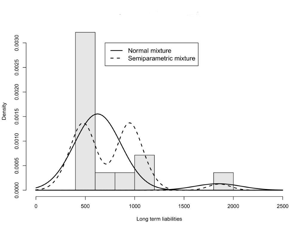
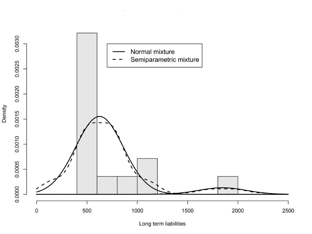
Figure 4: Histogram of Enron long term liabilities (in EUR) fitted with the 2-components Normal mixture (solid line) and the semiparametric model (dashed line). The semiparametric model was estimated with (second row) and without (first row) specifying the initial mean values of the mixture components.

Therefore, we modelled the current and long term assets and liabilities using a two-component Normal mixture, since this was the best model to fit the marginals. For each single firm we report the estimates of the parameters (posterior means) of the corresponding mixture models in Table 3, together with the 95% credible intervals (in brackets).

Table 3: Parameter estimates (posterior means) of the marginal distributions. The 95% credible intervals are in brackets.

Cirio	$\eta_{1}$	$\eta_{2}$	$\mu_{1}$	$\mu_{2}$	$\sigma^{2}$
$F_{A_{C}}$	0.635 (0.5386; 0.7241)	0.365 (0.2759; 0.4614)	40.28 (35.78; 44.56)	111.68 (105.93; 117.92)	272.94 (207.36; 360.09)
$F_{A_{L}}$	0.5096 (0.4156; 0.6009)	0.4904 (0.3991; 0.5844)	18.95 (17.51; 20.38)	37.84 (36.40; 39.24)	26.261 (19.19; 36.50)
$F_{B_{C}}$	0.5012 (0.4091; 0.5923)	0.4988 (0.4077; 0.5909)	39.54 (36.42; 42.68)	106.43 (103.16; 109.57)	163.79 (126.2; 212.4)
$F_{B_{L}}$	0.6954 (0.6101; 0.7757)	0.3046 (0.2243; 0.3899)	16.7 (14.52; 18.89)	67.24 (63.71; 70.56)	100.82 (77.44; 130.77)
Enron	$\eta_{1}$	$\eta_{2}$	$\mu_{1}$	$\mu_{2}$	$\sigma^{2}$
$F_{A_{C}}$	0.92336 (0.88023; 0.9598)	0.07664 (0.04022; 0.1198)	251.3 (227.7; 274.5)	2531.6 (2454.8; 2612.7)	21412 (17207; 26786)
$F_{A_{L}}$	0.7133 (0.6439; 0.7791)	0.2867 (0.2209; 0.3561)	556.9 (547.6; 566.3)	880.7 (865.5; 896.4)	2834.1 (2267.8; 3532.1)
$F_{B_{C}}$	0.92334 (0.87994; 0.9586)	0.07666 (0.04143; 0.1201)	260.7 (239.9; 280.7)	2367.4 (2296.5; 2438.5)	17062 (13768; 21157)
$F_{B_{L}}$	0.92231 (0.87554; 0.9576)	0.07769 (0.04236; 0.1245)	623.7 (588.7; 660.5)	1843.9 (1693.9; 1990.2)	56107 (44994; 69076)
Parmalat	$\eta_{1}$	$\eta_{2}$	$\mu_{1}$	$\mu_{2}$	$\sigma^{2}$
$F_{A_{C}}$	0.615 (0.5396; 0.6893)	0.385 (0.3107; 0.4604)	121.9 (109.2; 134.5)	386.3 (369.7; 403.4)	3852.4 (3044.4; 4815.9)
$F_{A_{L}}$	0.5375 (0.4658; 0.6084)	0.4625 (0.3916; 0.5342)	63.7 (58.85; 68.43)	175.2 (170.14; 180.50)	535.47 (425.71; 666.26)
$F_{B_{C}}$	0.92823 (0.88568; 0.9618)	0.07177 (0.03821; 0.1143)	194.3 (170.9; 217.2)	1587.8 (1500.4; 1674.0)	23362 (18985; 28988)
$F_{B_{L}}$	0.9278 (0.8882; 0.9616)	0.0722 (0.0384; 0.1118)	194 (170.3; 216.3)	1588.8 (1500.4; 1675.5)	23228 (19097; 28716)
Swissair	$\eta_{1}$	$\eta_{2}$	$\mu_{1}$	$\mu_{2}$	$\sigma^{2}$
$F_{A_{C}}$	0.5442 (0.4612; 0.6216)	0.4558 (0.3784; 0.5388)	162.5 (154.5; 171.8)	297.1 (288.6; 306.2)	1214.3 (923.6; 1609.7)
$F_{A_{L}}$	0.2339 (0.1696; 0.3034)	0.7661 (0.6966; 0.8304)	90.83 (79.09; 103.1)	349.66 (343.10; 356.3)	1373.1 (1104.6; 1731.0)
$F_{B_{C}}$	0.91266 (0.86004; 0.9524)	0.08734 (0.04762; 0.1400)	176.4 (169.4; 183.6)	350.5 (319.9; 378.6)	1901.9 (1502.5; 2405.3)
$F_{B_{L}}$	0.5402 (0.4606; 0.6183)	0.4598 (0.3817; 0.5394)	163.4 (148.8; 177.8)	439.5 (424.7; 455.0)	4259 (3345; 5412)
Sysco	$\eta_{1}$	$\eta_{2}$	$\mu_{1}$	$\mu_{2}$	$\sigma^{2}$
$F_{A_{C}}$	0.562 (0.4974; 0.6262)	0.438 (0.3738; 0.5026)	347.9 (323.5; 372.7)	811.2 (782.5; 839.5)	16877 (13847; 20727)
$F_{A_{L}}$	0.5649 (0.5061; 0.6248)	0.4351 (0.3752; 0.4939)	272.3 (251.9; 291.7)	830.9 (807.2; 854.0)	14281 (11983; 17031)
$F_{B_{C}}$	0.5005 (0.4401; 0.5637)	0.4995 (0.4363; 0.5599)	184.3 (171.8; 197.0)	518.0 (504.7; 531.2)	4982.4 (4177.6; 5903.8)
$F_{B_{L}}$	0.6356 (0.5760; 0.6945)	0.3644 (0.3055; 0.4240)	187.9 (174.2; 201.3)	546.3 (526.0; 565.4)	6875.2 (5765.7; 8190.0)

The classification probabilities $\eta_{p}$ are quite close to $0.5$ for Cirio data, for the asset marginals of Parmalat data, for the current assets and long term liabilities of Swissair data, and for Sysco data, denoting a balanced number of observations in the two mixture components. On the contrary, Enron data, the liability marginals of Parmalat data, long term assets and current liabilities of Swissair data show very different classification probabilities $\eta_{1}$ and $\eta_{2}$. This means that different proportions of observations are allocated to the components of the mixture and that one of the two components captures the greatest number of data. The location parameters of the two Normal components of the mixture $\mu_{p}$ are well separated, especially for Enron, Parmalat and Sysco, denoting that the mixture model is able to express the mean difference between the two components. The dispersion parameter $\sigma^{2}$ is particularly high for Enron, Parmalat and Sysco, while it is lower for Cirio and Swissair.

Enron and Parmalat have the most unbalanced mixture components, especially with reference to the liability marginal data. The data of these two companies are characterised by very different values of classification probabilities $\eta_{p}$, very different means $\mu_{p}$, and very high normal variance values $\sigma^{2}$. The resemblance of the structure of assets and liabilities in Enron and Parmalat may be explained by the similar behavior of these two companies during the years before their default. Parmalat indeed has been referred to as the “Europe’s Enron”.

We now present a graphical analysis of the results of Enron company. We have performed a similar analysis for the remaining four companies, but we do not report it here for lack of space.

Figure 5 shows the histograms of each marginal measured in EUR (grey bars), fitted with the location-shift model of two Normal components (black and grey lines) described in Section 4.1. $F_{A_{C}}$ is displayed in the top left panel, $F_{A_{L}}$ in the top right, $F_{B_{C}}$ in the bottom left and $F_{B_{L}}$ in the bottom right. Let us consider the picture related to the current assets marginal of Enron data (top left panel of Figure 5). The histogram shows a highly bimodal distribution which justifies the use of a finite mixture model. Similar comments arise from the analysis of the fitted histograms of the remaining marginals.

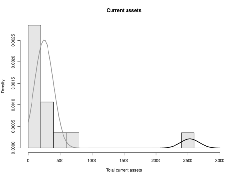
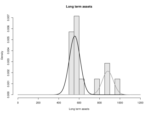
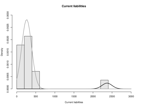
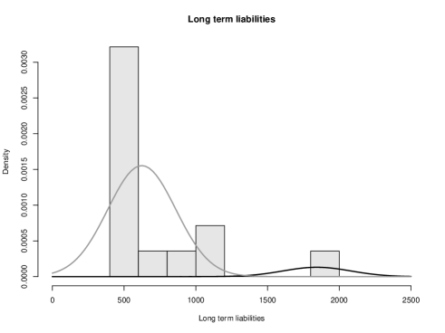
Figure 5: Enron data, measured in EUR, fitted with a mixture of two Normal components: $F_{A_{C}}$ (top left), $F_{A_{L}}$ (top right), $F_{B_{C}}$ (bottom left) and $F_{B_{L}}$ (bottom right).

Figure 6 shows the sampled values of the $\mu_{1}$ parameter on the horizontal axis and of the $\mu_{2}$ parameter on the vertical axis. $F_{A_{C}}$ is displayed in top left panel, $F_{A_{L}}$ in the top right, $F_{B_{C}}$ in the bottom left and $F_{B_{L}}$ in the bottom right. It is interesting to note that our data are not affected by label switching, since the segments are rather well separated for $\mu$, as there are no points on the diagonal on the $\mu_{1}$ versus $\mu_{2}$ plots.

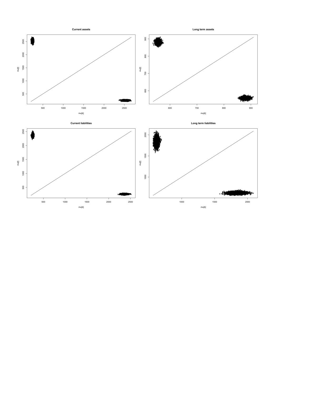
Figure 6: Enron data: $\mu_{1}$ versus $\mu_{2}$. $F_{A_{C}}$ is in the top left, $F_{A_{L}}$ is in the top right, $F_{B_{C}}$ is in the bottom left and $F_{B_{L}}$ is displayed in the bottom right panel.

Focusing on the MCMC results, here we illustrate the outcomes of the Enron long term assets data, since the results of the remaining marginals are very similar to those presented. Figures 7, 8 and 9 depict MCMC trace plots and posterior densities, obtained using kernel density estimation from the R package “bayesmix” of Grüen (2014), for the parameters $\eta$, $\mu$ and $\sigma^{2}$, respectively. We run the algorithm for 4,000 iterations, discarding the first 1,000 iterations as burn-in period. The trace plots show that the chains are well mixing, exploring freely the sample space and clearly reaching convergence to the target distribution. Moreover, the unidentifiability problem due to label switching, that may lead to biased estimates, in our case does not occur. Finally, the posterior density plots have regular forms and do not show multimodalities.

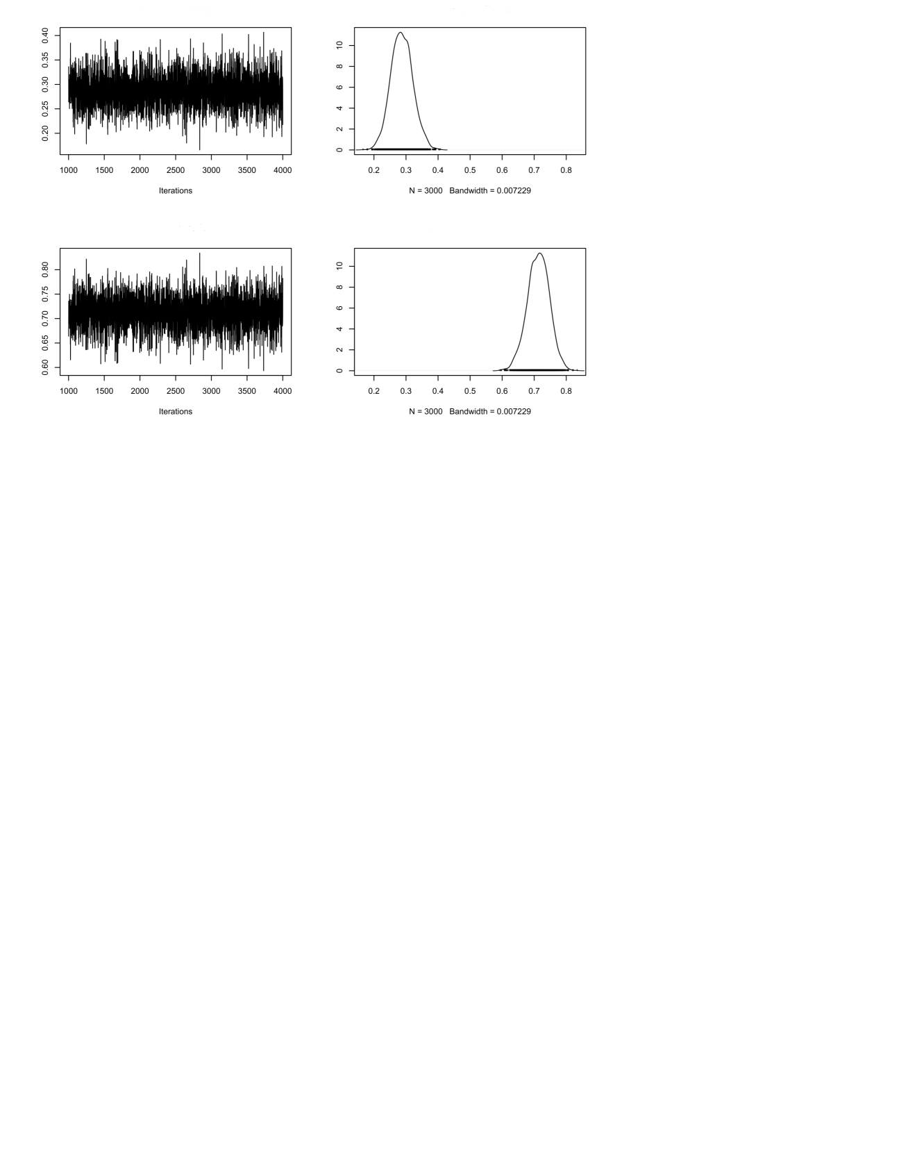
Figure 7: Enron long term assets data: MCMC traces (left panels) and posterior densities (right panels) for $\eta$; with $\eta_{1}$ on the first row and $\eta_{2}$ on the second row.

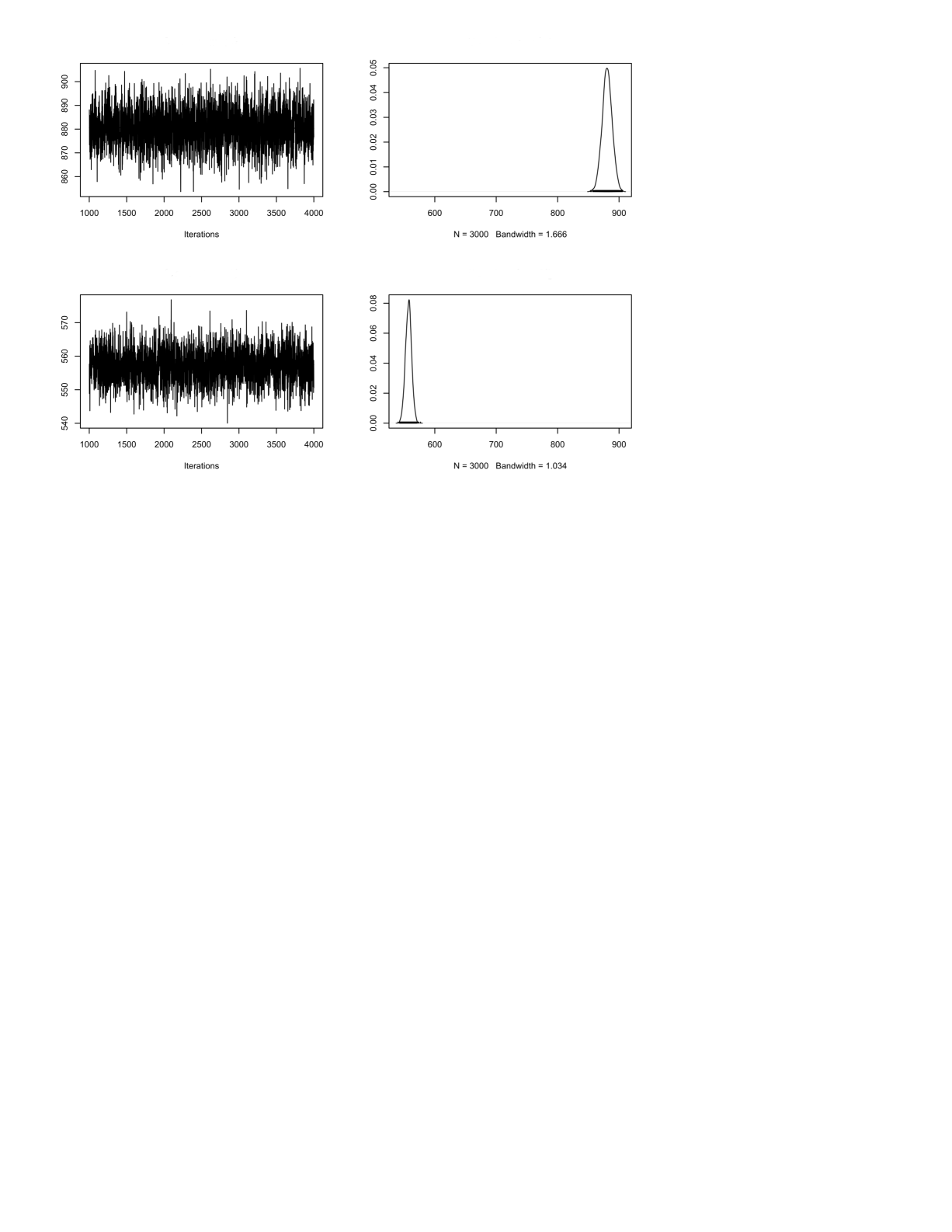
Figure 8: Enron long assets data: MCMC traces (left panels) and posterior densities (right panels) for $\mu$; with $\mu_{1}$ on the first row and $\mu_{2}$ on the second row.

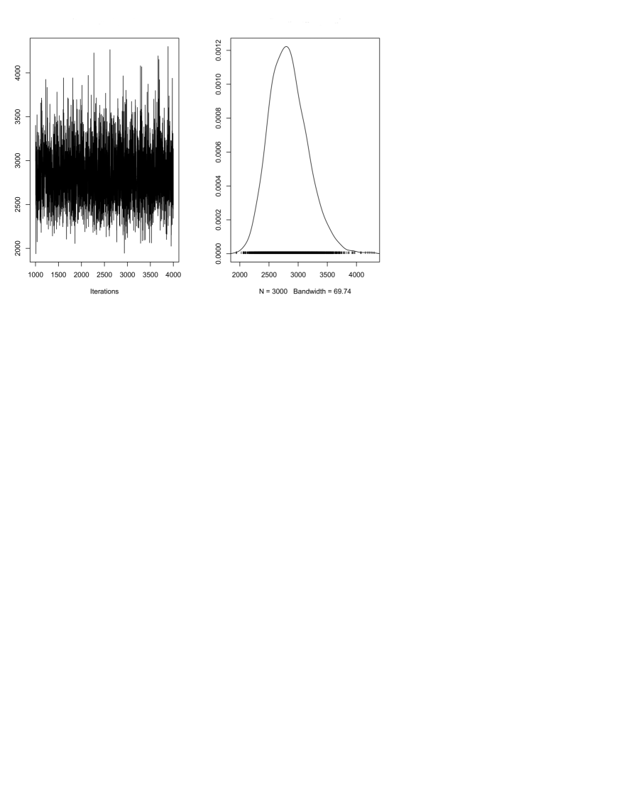
Figure 9: Enron long term assets data: MCMC trace (left panel) and posterior density (right panel) for $\sigma^{2}$.

5.2 PCC for Asset and Liability Data

Following the procedure described in Section 4.2 we select an appropriate pair copula decomposition for the D-vine. For each one of the defaulted firms the order of the marginals that maximizes the pairwise Kendall’s $\tau$ indexes in the first tree is $A_{C_{T}}\hskip 2.84544pt-\hskip 2.84544ptB_{C_{T}}\hskip 2.84544pt-\hskip 2.84544ptB_{L_{T}}\hskip 2.84544pt-\hskip 2.84544ptA_{L_{T}}.$

In Tables 4, 5, 6 and 7 we display, for the defaulted firms, the list of pair copulas for each D-vine, the selected copula families, the copula parameters (one or two according to the type of copula) and the corresponding Kendall’s $\tau$. The results are obtained using the R package “CDVine” by Brechmann and Schepsmeier (2013). From the selected copula families, we see evidence of different types of asymmetric dependence. This demonstrates that the choice of PCCs is appropriate, since it guarantees enough flexibility to model the complex and asymmetric dependence structure of the data at hand. Note that only the Cirio D-vine (Table 4) has none conditional independent variable pairs. For these data the Genest and Favre (Genest and Favre (2007)) independence test rejected independency for all the copulas involved. An independence copula has been selected instead for $c_{A_{C_{T}},B_{L_{T}}|B_{C_{T}}}$ in the second tree for Parmalat and Swissair (Tables 6 and 7), while $c_{A_{L_{T}},B_{C_{T}}|B_{L_{T}}}$ has been identified as an independence copula for Enron (Table 5). In these cases the D-vine structure is simplified and we do not need to estimate the parameters of the copula $c_{A_{C_{T}},A_{L_{T}}|B_{C_{T}},B_{L_{T}}}$ in the third tree. The presence of conditional independence in this last case suggests a weak relationship between the current and long term assets, given the values of liabilities. From the unconditional pair copulas, we note an existing dependence between current and long term assets or liabilities, and also a dependence between the two different types of liabilities. A strong dependence in conditional copulas instead may suggest imbalance, when current assets are financed by long term liabilities, or a serious liquidity problem, when long term assets are financed by current liabilities. These situations need particular attention, because they may prelude to the default of the firm.

For the Sysco company the order in the first tree is $A_{C_{T}}\hskip 2.84544pt-\hskip 2.84544ptA_{L_{T}}\hskip 2.84544pt-\hskip 2.84544ptB_{L_{T}}\hskip 2.84544pt-\hskip 2.84544ptB_{C_{T}}.$ In Table 8 we display the list of pair copulas for the D-vine, the selected copula families, the copula parameters (one or two according to the type of copula) and the corresponding Kendall’s $\tau$. In this case, an independence copula has been selected for $c_{A_{C_{T}},B_{L_{T}}|A_{L_{T}}}$. The D-vine structure is simplified and we do not need to estimate the parameters of the copula $c_{A_{C_{T}},B_{C_{T}}|A_{L_{T}},B_{L_{T}}}$ in the third tree. The presence of conditional independence in this last case suggests a weak relationship between the current asset and liabilities, given the values of the long term ones.

Table 4: Cirio: selected copulas and D-vine PCC parameters. SBB1, BB7 and BB8 are, respectively, the Survival Clayton-Gumbel, the Joe-Clayton and the Joe-Frank copulas, that are Archimedean copula families with two parameters.

Cirio: Pair Copula Parameters of the D-Vine
Copulas	family	parameter 1	parameter 2	Kendall’s $\tau$
$c_{A_{C_{T}},B_{C_{T}}}$	SBB1	0.0010	3.3814	0.7044
$c_{B_{C_{T}},B_{L_{T}}}$	BB8	1.2579	0.9902	0.1186
$c_{B_{L_{T}},A_{L_{T}}}$	BB7	1.1195	4.7016	0.6985
$c_{A_{C_{T}},B_{L_{T}}|B_{C_{T}}}$	Frank	7.2222	N/A	0.5718
$c_{A_{L_{T}},B_{C_{T}}|B_{L_{T}}}$	Normal	-0.0337	N/A	-0.0214
$c_{A_{C_{T}},A_{L_{T}}|B_{C_{T}},B_{L_{T}}}$	Frank	-8.9557	N/A	-0.6353

Table 5: Enron: selected copulas and D-vine PCC parameters. SBB8 and BB8 are, respectively, the Survival Joe-Frank and the Joe-Frank copulas, Archimedean copula families with two parameters.

Enron: Pair Copula Parameters of the D-Vine
Copulas	family	parameter 1	parameter 2	Kendall’s $\tau$
$c_{A_{C_{T}},B_{C_{T}}}$	Student’s t	0.9868	7.6539	0.8963
$c_{B_{C_{T}},B_{L_{T}}}$	SBB8	6.0000	0.3924	0.2761
$c_{B_{L_{T}},A_{L_{T}}}$	BB8	5.9831	0.9979	0.7208
$c_{A_{C_{T}},B_{L_{T}}|B_{C_{T}}}$	Rotated Clayton	-1.4730	N/A	-0.4241
$c_{A_{L_{T}},B_{C_{T}}|B_{L_{T}}}$	Independence	N/A	N/A	0

Table 6: Parmalat: selected copulas and D-vine PCC parameters. BB1 is the Clayton-Gumbel copula, Archimedean copula family with two parameters.

Parmalat: Pair Copula Parameters of the D-Vine
Copulas	family	parameter 1	parameter 2	Kendall’s $\tau$
$c_{A_{C_{T}},B_{C_{T}}}$	BB1	0.4325	4.2015	0.8043
$c_{B_{C_{T}},B_{L_{T}}}$	Normal	0.9998	N/A	0.9898
$c_{B_{L_{T}},A_{L_{T}}}$	Clayton	1.2256	N/A	0.3800
$c_{A_{C_{T}},B_{L_{T}}|B_{C_{T}}}$	Independence	N/A	N/A	0
$c_{A_{L_{T}},B_{C_{T}}|B_{L_{T}}}$	Frank	-7.3657	N/A	-0.5778

Table 7: Swissair: selected copulas and D-vine PCC parameters. BB7 and SBB8 are, respectively, the Joe-Clayton and the Survival Joe-Frank copula, Archimedean copula families with two parameters

Swissair: Pair Copula Parameters of the D-Vine
Copulas	family	parameter 1	parameter 2	Kendall’s $\tau$
$c_{A_{C_{T}},B_{C_{T}}}$	BB7	2.4309	5.3880	0.7267
$c_{B_{C_{T}},B_{L_{T}}}$	SBB8	1.0081	1.0000	0.0047
$c_{B_{L_{T}},A_{L_{T}}}$	BB7	1.0010	2.9494	0.5959
$c_{A_{C_{T}},B_{L_{T}}|B_{C_{T}}}$	Independence	N/A	N/A	0
$c_{A_{L_{T}},B_{C_{T}}|B_{L_{T}}}$	Rotated Joe	-2.3405	N/A	-0.4222

Table 8: Sysco: selected copulas and D-vine PCC parameters. BB1 and BB6 are, respectively, the Clayton-Gumbel and the Survival Joe-Gumbel copulas, that are Archimedean copula family with two parameters.

Sysco: Pair Copula Parameters of the D-Vine:
Copulas	family	parameter 1	parameter 2	Kendall’s $\tau$
$c_{A_{C_{T}},A_{L_{T}}}$	BB6	6	1.9387	0.8569
$c_{A_{L_{T}},B_{L_{T}}}$	Frank	298.314	N/A	0.9867
$c_{B_{L_{T}},B_{C_{T}}}$	BB1	4.4714	1.7693	0.8253
$c_{A_{C_{T}},B_{L_{T}}|A_{L_{T}}}$	Independence	N/A	N/A	0
$c_{A_{L_{T}},B_{C_{T}}|B_{L_{T}}}$	Normal	-0.0270	N/A	-0.0172

5.3 Probability of Default Estimation

To estimate the PD we follow the methodology described in Section 3.2. For each firm we generate 10,000 simulations from the selected D-vine to obtain the equity distribution and the PD. Figure 10 depicts the equity densities of Cirio, Enron, Parmalat, Swissair and Sysco, respectively on the top left, top right, middle left, middle right and bottom panel. The Figure was obtained using kernel density estimation. The value of the PD is written in the relevant plot and corresponds to the area under the curve where the equity is zero or negative. The PD values are very high for all defaulted firms, lying in the range $0.4468-0.6892$; in contrast, the Sysco PD is only $0.0026$, as we expected for a healthy company, where the probability of going bankrupt is very low. We notice that the PD values of Enron and Swissair are slightly lower than the other defaulted firms. However, the available balance sheet data did not include the last year of activity of Enron and Swissair. This might have affected the final results, since the inclusion of the last year’s data would certainly have increased the corresponding PD values.

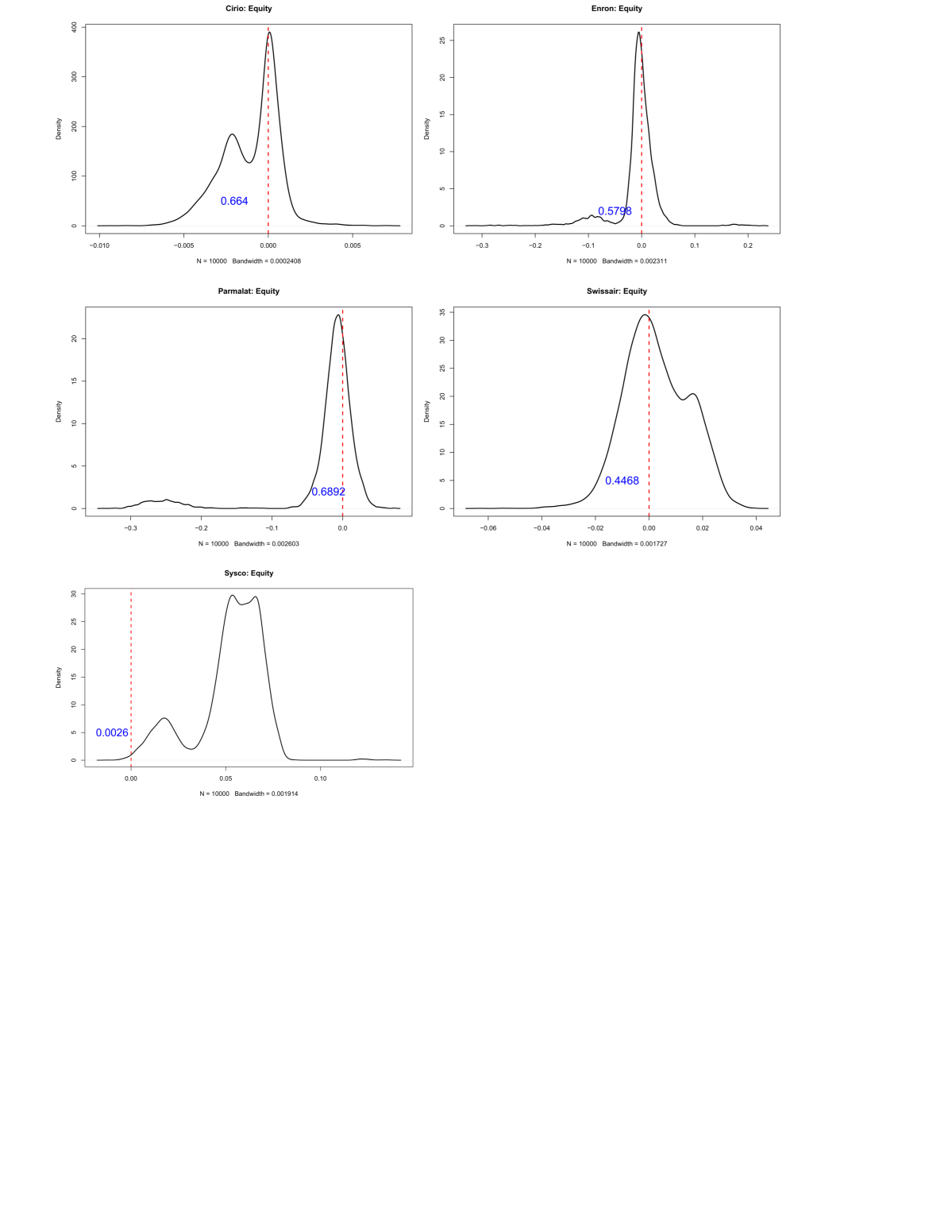
Figure 10: Equity densities of Cirio (top left), Enron (top right), Parmalat (middle left), Swissair (middle right) and Sysco (bottom). The value of the PD is written on the corresponding densities.

For comparative purposes we contrasted our results with those obtained applying the original Z-score proposed by Altman (1968), e.g. to the Enron company.

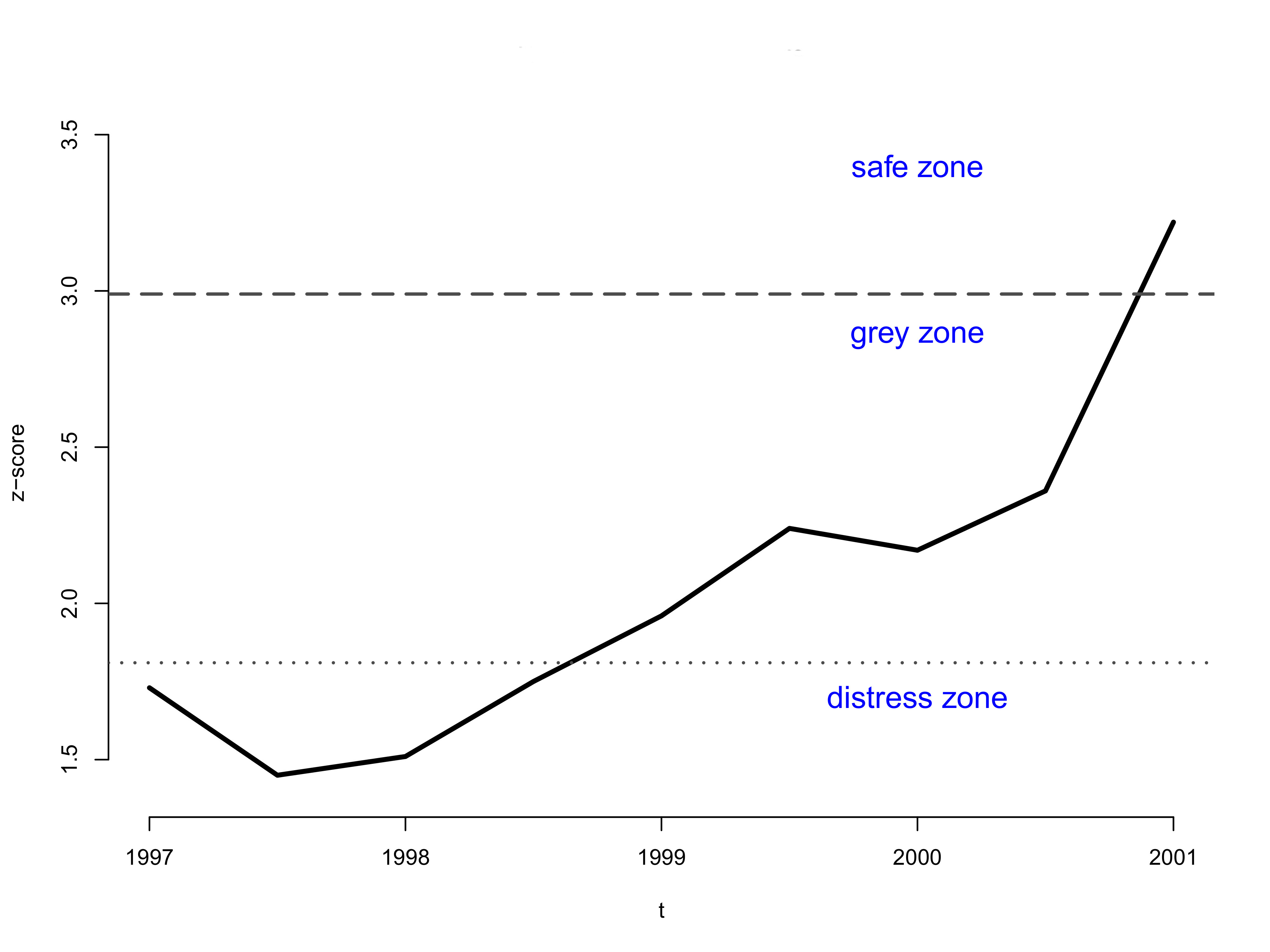
Figure 11: Altman’s Z-score for Enron data

Figure 11 shows the line plot of Altman’s Z-score for the time horizon between 1997 and 2001. According to Altman (1968), a company is considered to be in the “safe” zone (healthy) when $z>2.99$, it is in the “grey” zone (moderate risk of default) when $1.81<z<2.99$, and it is in the “distress” zone (high danger of default) when $z<1.81$. Altman’s Z-score is clearly not able to predict the failure of the Enron company, since it locates the firm in the distress zone only until 1998; subsequently, from 1999 to 2000, it moves the firm to the grey zone (erroneously suggesting an improved performance); and finally (when the actual default actually occurred) places the firm in the safe area, with a z-score of 3.22. Besides, in the considered period Altman’s Z-score is not decreasing, but even rising, leading to completely misleading conclusions.

The Z-score’s inability of predicting the default is due to the fact that, unlike the PCC model, it does not consider the dependence pattern among the different components of the balance sheet data. On the contrary, the proposed PCC model allows us to measure the dependencies and to detect in advance alarming situations, which are not identifiable using other traditional models. Moreover, our PCC approach permits to adopt different and more suitable marginal distributions, better reflecting the structure of the data at hand.

Moreover, the calculation of Altman’s Z-score, unlike the PCC model, involves balance sheet data as well as economic and income data, without analysing the relationship among these quantities. For this reason, the Z-score might mask dangerous default risks, classifying a company as “safe”, when it is truly in distress.

6 Summary and Conclusions

The aim of this paper was to propose a novel methodology for PD evaluation. Our final goal was to calculate the PD of large firms using their balance sheet data. We measured the firm value via a contingent claim, whose pricing function may be expressed using copulas. The marginals are given by the current and long term assets and liabilities. Hence, the equity function is expressed by a 4-dimensional D-vine copula. To test the performance of our methodology we applied it to four fraudulent defaulted stocks and to the data of a healthy firm. In order to estimate the marginals we employed a Bayesian mixture model, able to model the presence of two clusters in the asset as well as liability data. The structure of the marginals in defaulted firms reflects the choices of the management, trying to balance high and low accounting items during the period before the default. Considering the copula, we chose to employ PCCs, because they allow for a great flexibility in modelling the dependence structure of the marginals. As demonstrated by the results, the pair copulas selected in the D-vines belong to different families and describe various types of dependence. The analysis of these dependencies in defaulted firms data already reveals substandard loans and situations of serious imbalance due to liquidity issues, especially when the firm tries to balance long term assets with current liabilities. Finally, we calculated the PD of the five considered firms, simulating from the D-vines and obtaining the equity distributions. The final results show a high PD for the defaulted firms, suggesting their forthcoming bankruptcy. The PD of the Sysco company is instead much lower than those of the defaulted firms, denoting a good performance. A traditional indicator like Altman’s Z-score may be incapable of predicting the risk of default, since it is not flexible enough and it does not incorporate the dependence structure of the involved quantities. On the contrary, the proposed methodology has proven to be successful in the evaluation of PD and would certainly benefit analysts and managers, advising them to take actions against a potential bankruptcy.

Possible extensions of our work include the estimation of the whole model in a full Bayesian framework, the application of nonparametric approaches for PCCs, the use of balance indicators instead of accounting items and the use of a our methodology to analyze the contagion in sectors of activity. Finally, it would be interesting to apply our approach to Altman’s Z-score, to model the dependence between the different quantities involved.

References

- Aas and Berg (2009) Aas, K., & Berg, D. (2009). Models for construction of multivariate dependence - a comparison study. The European Journal of Finance, 15, 639–659.
- Aas et al. (2009) Aas, K., Czado, C., Frigessi, A., & Bakken, H. (2009). Pair-copula constructions of multiple dependence. Insurance: Mathematics and Economics, 44, 182–198.
- Allen et al. (2013) Allen, D. E., Ashraf, M. A., McAleer, M., Powell, R. J., & Singh, A. K. (2013). Financial dependence analysis: applications of vine copulas. Statistica Neerlandica, 67, 403–435.
- Altman (1968) Altman, E. (1968). Financial Ratios, Discriminant Analysis and the Prediction of Corporate Bankruptcy. Journal of Finance, 23, 589–609.
- Altman et al. (2011) Altman, E., Fargher, N., & Kalotay, E. (2011). A Simple Empirical Model of Equity-Implied Probabilities of Default. The Journal of Fixed Income, 20, 71–85.
- Bauer et al. (2012) Bauer, A., Czado, C., & Klein, T. (2012). Pair-copula constructions for non-Gaussian DAG models. Canadian Journal of Statistics, 40, 86–109
- Beaver (1968) Beaver, W. (1968). Market Prices, Financial Ratios, and the Prediction of Failure. Journal of Accounting Research, 8, 179–192.
- Bedford and Cooke (2001) Bedford, T., & Cooke, R.M. (2001). Probability density decomposition for conditionally dependent random variables modeled by vines. Annals of Mathematics and Artificial Intelligence, 32, 245–268.
- Bedford and Cooke (2002) Bedford, T., & Cooke, R.M. (2002). Vines - a new graphical model for dependent random variables. Annals of Statistics, 30, 1031–1068.
- Benaglia et al. (2009) Benaglia, T., Chauveau, D., Hunter, D. , & Young, D. (2009). mixtools: An R Package for Analyzing Finite Mixture Models. Journal of Statistical Software, 32, 1–29.
- Bernard and Czado (2013) Bernard, C., & Czado, C. (2013). Multivariate option pricing using copulae. Applied Stochastic Models in Business and Industry, 29, 509–526.
- Bharath and Shumway (2008) Bharath, S. T., & Shumway, T. (2008). Forecasting Default with the Merton Distance to Default Model. Review of Financial Studies, 21, 1339–1369.
- Bhimani et al. (2014) Bhimani, A., Gulamhussen, M.A., & da Rocha Lopes, S. (2014). Owner liability and financial reporting information as predictors of firm default in bank loans. Review of Accounting Studies, 19, 769–804.
- Black and Scholes (1973) Black, F., & Scholes M. (1973). The Pricing of Options and Corporate Liabilities. Journal of Political Economy, 81, 637–654.
- Bo et al. (2011) Bo, L., Tang, D., Wang, Y., & Yang, X. (2011). On the conditional default probability in a regulated market: a structural approach. Quantitative Finance, 11, 1695–1702.
- Bo et al. (2013) Bo, L., Li, X., Wang, Y., & Yang, X. (2013). On the conditional default probability in a regulated market with jump risk. Quantitative Finance, 13, 1967–1975.
- Bordes et al. (2006) Bordes, L., Mottelet, S., & Vandekerkhove, P. (2006). Semiparametric Estimation of a Two-Component Mixture Model. The Annals of Statistics, 34, 1204–1232.
- Brechmann (2010) Brechmann, E. C. (2010). Truncated and simplified regular vines and their applications, Diploma thesis, Technische Universität München.
- Brechmann and Schepsmeier (2013) Brechmann, E.C., & Schepsmeier, U. (2013). Modeling Dependence with C- and D-Vine Copulas: The R Package CDVine. Journal of Statistical Software, 52, 1–27.
- Clarke (2007) Clarke, K.A. (2007). A Simple Distribution-Free Test for Nonnested Model Selection. Political Analysis, 15, 347–363.
- Czado (2010) Czado, C. (2010). Pair-Copula Constructions of Multivariate Copulas. In Copula Theory and its Applications, Lecture Notes in Statistics, 198, Springer, 93–109.
- De Giuli et al. (2008) De Giuli, M.E., Fantazzini, D., & Maggi, M.A. (2008). A New Approach for Firm Value and Default Probability Estimation beyond Merton Models. Computational Economics, 31, 161–180.
- Dißmann et al. (2013) Dißmann, J., Brechmann, E., Czado, C., & Kurowicka, D. (2013). Selecting and estimating regular vine copulae and application to financial returns. Computational Statistics & Data Analysis, 59, 52–69.
- Eberhart (2005) Eberhart, A.C. (2005). A comparison of Merton’s option pricing model of corporate debt valuation to the use of book values. Journal of Corporate Finance, 11, 401–426.
- Escobar and West (1995) Escobar, M.D., & West, M. (1995). Bayesian density estimation and inference using mixtures. Journal of the American Statistical Association, 90, 577–588.
- Genest and Favre (2007) Genest, C., & Favre, A.C. (2007). Everything you always wanted to know about copula modeling but were afraid to ask. Journal of Hydrologic Engineering, 12 , 347–368.
- Grüen (2014) Grüen, B. (2014). bayesmix: Bayesian Mixture Models with JAGS. R package version 0.7-3. http://CRAN.R-project.org/package=bayesmix.
- Haff et al. (2010) Haff, I.H., Aas, K., & Frigessi, A. (2010). On the simplified pair-copula construction - simply useful or too simplistic? Journal of Multivariate Analysis, 101, 1296–1310.
- Haff and Segers (2015) Haff, I.H., & Segers, J. (2015). Nonparametric estimation of pair-copula constructions with the empirical pair-copula. Computational Statistics & Data Analysis, 84, 1–13.
- Hunter et al. (2007) Hunter, D.R., Wang, S., & Hettmansperger, T.P. (2007). Inference for Mixtures of Symmetric Distributions. The Annals of Statistics, 35, 224–251.
- Jaworski (2010) Jaworski, P. (2010). Tail behaviour of copula. In Copula Theory and its Applications, Lecture Notes in Statistics, 198, Springer, 161–186.
- Ji (2010) Ji, H. (2010). The Structural Approach to Modeling Credit Risk. In Handbook of Quantitative Finance and Risk Management, edited by C.F. Lee, A. C. Lee, and John Lee, Springer Verlag, 665–673.
- Joe (1996) Joe, H. (1996). Families of m-variate distributions with given margins and m(m-1)/2 bivariate dependence parameters. IMS Lecture Notes-Monograph Series, 28, 120–141.
- Joe (1997) Joe, H. (1997). Multivariate model and dependence concepts, Monographs on Statistics an Applied Probability, 73, Chapman , Hall, London.
- Joe and Xu (1996) Joe, H., & Xu, J. (1996). The estimation method of inference functions for margins for multivariate models. Technical Report 166, Department of Statistics, University of British Columbia.
- Kass and Raftery (1995) Kass, R., & Raftery, A. (1995). Bayes factors. Journal of the American Statistical Association, 90, 773–795.
- Kauermann et al. (2013) Kauermann, G., Schellhase, C., & Ruppert, D. (2013). Flexible Copula Density Estimation with Penalized Hierarchical B-Splines. Scandinavian Journal of Statistics, 40, 685 -705.
- Kazemi and Mosleh (2012) Kazemi, R., & Mosleh, A. (2012). Improving Default Risk Prediction Using Bayesian Model Uncertainty Techniques. Risk Analysis, 32, 1888–1900.
- Kiefer (2009) Kiefer, N.M. (2009). Default estimation for low-default portfolios. Journal of Empirical Finance, 16, 164–173.
- Kiefer (2010) Kiefer, N.M. (2010). Default Estimation and Expert Information. Journal of Business, Economic Statistics, 28, 320–328.
- Kiefer (2011) Kiefer, N. M. (2011). Default estimation, correlated defaults, and expert information. Journal of Applied Economics, 26, 173–192.
- Komarek and Lesaffre (2008) Komarek, A., & Lesaffre, E. (2008). Generalized linear mixed model with a penalized gaussian mixture as random effects distribution. Computational Statistics & Data Analysis, 52, 3441–3458.
- Kreinin and Nagi (2008) Kreinin, A., & Nagi, A. (2008). Calibration of the default probability model. European Journal of Operational Research, 185, 1462–1476.
- Kurowicka and Cooke (2006) Kurowicka, D., & Cooke, R. (2006). Unceirtanty analysis with high dimensional dependence modelling, Wiley, Chichester.
- Laajimi (2012) Laajimi, S. (2012). Structural Credit Risk Models: A Review. Insurance and Risk Management, 80, 53–93.
- Leow and Crook (2015) Leow, M. & Crook, J. (in press, 2015). The stability of survival model parameter estimates for predicting the probability of default: Empirical evidence over the credit crisis. European Journal of Operational Research.
- Liebscher (2006) Liebscher, E. (2006). Modelling and estimation of multivariate copulas. Working paper, University of Applied Sciences Merseburg, Germany.
- Liu et al. (2015) Liu, F., Hua, Z., & Lim, A. (2015). Identifying future defaulters: A hierarchical Bayesian method. European Journal of Operational Research, 241, 0377–2217.
- Marin et al. (2005) Marin, J.M., Mengersen, K.L., & Robert C.P. (2005). Bayesian modelling and inference on mixtures of distributions. Handbook of Statistics, 25, Springer-Verlag, New York.
- McLachlan and Peel (2000) McLachlan, G., & Peel, D. (2000). Finite Mixture Models, Wiley, New York.
- Merton (1970) Merton, R.C. (1970). A dynamic general equilibrium model of the asset market and its application to the pricing of the capital structure of the firm. MIT Sloan School of Management Working Paper Series, 497–70, Massachusetts. Institute of Technology, Cambridge, MA.
- Merton (1974) Merton, R. C. (1974). On the pricing of corporate debt: The risk structure of interest rates. Journal of Finance, 29, 449–470.
- Merton (1977) Merton, R. C. (1977). On the pricing of contingent claims and the Modigliani-Miller theorem. Journal of Financial Economics, 15, 241–250.
- Min and Czado (2010) Min, A., & Czado, C. (2010). Bayesian inference for multivariate copulas using pair-copula constructions. Journal of Financial Econometrics, 8, 511–546.
- Morales-Napoles (2011) Morales-Napoles, O. (2011). Counting vines. In Dependence Modeling: Vine Copula Handbook, Kurowicka and Joe (Eds.), World Scientific Publishing Co.
- Morillas (2005) Morillas, P. (2005). A method to obtain new copulas from a given one. Metrika, 61, 169–184.
- Müller et al. (2015) Müller, P., Quintana, F.A., Jara, A. & Hanson, T. (2015). Bayesian Nonparametric Data Analysis, Springer, Switzerland.
- Nelsen (1999) Nelsen, R. B. (1999). An introduction to copulas, Springer-Verlag, New York.
- Nikoloulopoulos et al. (2012) Nikoloulopoulos, A.K., Joe, H., & Li, H. (2012). Vine copulas with asymmetric tail dependence and applications to financial return data. Computational Statistics & Data Analysis, 56, 3659–3673.
- Ohlson (1980) Ohlson, J. (1980). Financial ratios and the probability perdiction of bankruptcy. Journal of Accounting Research, 18, 109–131.
- Orth (2013) Orth, W. (2013). Default probability estimation in small samples with an application to sovereign bonds. Quantitative Finance, 13, 1891–1902.
- Park et al. (2010) Park, Y., Sirakaya, S., & Kim, T.Y. (2010). A Dynamic Hierarchical Bayesian Model for the Probability of Default. Working Paper, 98, Center for Statistics and the Social Sciences, University of Washington.
- Peel and McLachlan (2000) Peel, D., & McLachlan, G. (2000). Robust mixture modelling using the t distribution.Statistics and Computing, 10, 339 -348.
- Peterkort and Nielsen (2005) Peterkort, R.F., & Nielsen, J.F. (2005). Is book-to-market ratio a measure of risk? Journal of Financial Research, 28, 487–502.
- Plummer (2003) Plummer, M. (2003). JAGS: A program for analysis of Bayesian graphical models using Gibbs sampling. In Proceedings of the 3rd International Workshop on Distributed Statistical Computing, 20–22.
- Richardson and Green (1997) Richardson, S., & Green, P. (1997). On Bayesian analysis of mixtures with an unknown number of components. Journal of the Royal Statistical Society, Series B, 59, 731–792.
- Ronn and Verma (1986) Ronn, E.I., & Verma, A.K. (1986). Pricing Risk-Adjusted Deposit Insurance: an Option-Based Model. The Journal of Finance, 4, 871–895.
- Sancetta and Satchell (2004) Sancetta, A., & Satchell, S. (2004). Bernstein copula and its applications to modeling and approximations of multivariate distributions. Econometric Theory, 20, 535–562.
- Savu and Trede (2006) Savu, C., & Trede, M. (2006). Hierarchical Archimedean copulas. In International Conference on High Frequency Finance, Konstanz, Germany.
- Schellhase and Kauermann (2012) Schellhase, C., & Kauermann, G. (2012). Density estimation and comparison with a penalized mixture approach. Computational Statistics, 27, 757–777.
- Shen et al. (2008) Shen, X., Zhu, Y., & and Song, L. (2008). Linear B-spline copulas with applications to nonparametric estimation of copulas. Computational Statististics & Data Analysis, 52, 3806–3819.
- Sklar (1959) Sklar, M. (1959). Fonctions de répartition á ndimensions et leurs marges. Publications de l’Institut de Statistique de l’Université de Paris, 8, 229–231.
- Su and Huang (2010) Su, E.D., & Huang, S.N. (2010). Comparing Firm Failure Predictions Between Logit, KMV, and ZPP Models: Evidence from Taiwan’s Electronics Industry. Asia-Pacific Financial Markets, 17, 209–239.
- Sundaresan (2013) Sundaresan, S. (2013). A Review of Merton s Model of the Firm s Capital Structure with Its Wide Applications. Annual Review of Financial Economics, 5, 21–41.
- Tanner and Wong (1987) Tanner, M., & Wong, W. (1987). The calculation of posterior distributions by data augmentation. Journal of the American Statistical Association, 82, 528–550.
- Tasche (2011) Tasche, D. (2011). Bayesian estimation of probabilities of default for low default portfolios, arXiv:1112.5550v3.
- Tobback et al. (2014) Tobback, E., Martens, D., Van Gestel, T., & Baesens, B. (2014). Forecasting Loss Given Default models: impact of account characteristics and the macroeconomic state. Journal of the Operational Research Society, 65, 376–392.
- Vaz de Melo Mendes et al. (2010) Vaz de Melo Mendes, B., Mendes Semeraro, M., & Camara Leal, R. P. (2010). Pair-copulas modeling in finance. Financial Market and Portfolio Management, 24, 193–213.
- Vuong (1989) Vuong, Q.H. (1989). Ratio Tests for Model Selection and Non-Nested Hypotheses. Econometrica, 57, 307–333.
- Weiß and Scheffer (2012) Weiss, G., & Scheffer, M. (2012). Smooth nonparametric bernstein vine copulas, arXiv:1210.2043.
- Whelan (2004) Whelan, N. (2004). Sampling from Archimedean copulas. Quantitative Finance, 4, 339–352.