Proton polarizabilities from polarized Compton scattering: low-energy expansion

Abstract:

We reexamine the low-energy expansion of polarized Compton scattering off the proton and show that the leading non-Born contribution to the beam asymmetry of low-energy Compton scattering is given by the magnetic polarizability alone, the electric polarizability cancels out. Based on this fact we propose to determine the magnetic dipole polarizability of the proton from the beam asymmetry. We also present the low-energy expansion of doubly-polarized observables, from which the spin polarizabilities can be extracted.

Studies of nucleon polarizabilities have recently intensified fueled by theoretical advances based on chiral perturbation theory and the current experimental programs at MAMI, HIGS and CEBAF facilities, see Refs. [1, 2] for fresh reviews. As a result, the Particle Data Group (PDG) [3] has recently updated its summary of the dipole electric and magnetic polarizabilities of the proton, yielding [4]:

$$\alpha_{E1}^{(p)} = (12.0\pm 0.6)\times 10^{-4}\,\mbox{fm${}^{3}$},$$ (1a)

$$\beta_{M1}^{(p)} = (2.5\pm 0.4)\times 10^{-4}\,\mbox{fm${}^{3}$}.$$ (1b)

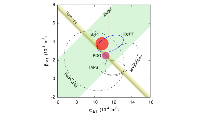
Figure 1: The scalar polarizabilities of the proton. Magenta blob represents the PDG summary [4] . Experimental results are from Federspiel et al. [12], Zieger et al. [13], MacGibbon et al. [14], and TAPS [15]. ‘Sum Rule’ indicates the Baldin sum rule evaluations of $\alpha_{E1}+\beta_{M1}$ [15] (broader band) and [16]. ChPT calculations are from [11] (B$\chi$PT—red blob) and the ‘unconstrained fit’ of [17] (HB$\chi$PT—blue ellipse).

These values, together with some other experimental and most recent theoretical results, are displayed in Fig. 1. As the figure shows, the various determinations of polarizabilities may differ by a few standard deviations. The main source of these discrepancies is the model dependence of the extraction of polarizabilities from the unpolarized Compton scattering cross sections. The forthcoming measurements of the beam asymmetry of proton Compton scattering are called for to sort out this issue [5].

Besides the two scalar polarizabilities, the four spin polarizabilities of the proton are of significant interest both theoretically and experimentally. New experiments at MAMI are aimed to determine them. Two combination of spin polarizabilities have been already determined, i.e. forward and backward spin polarizabilities [6]:

$$\gamma_{0} = -\gamma_{E1E1}-\gamma_{M1M1}-\gamma_{E1M2}-\gamma_{M1E2}=(-1.0\pm 0.08\pm 0.1)\times 10^{-4}\,\mathrm{fm}^{4},$$ (2)

$$\gamma_{\pi} = -\gamma_{E1E1}+\gamma_{M1M1}-\gamma_{E1M2}+\gamma_{M1E2}=(8.0\pm 1.8)\times 10^{-4}\,\mathrm{fm}^{4}.$$ (3)

Two more are soon to be measured at MAMI. We shall have a look here at observables relevant to these measurements.

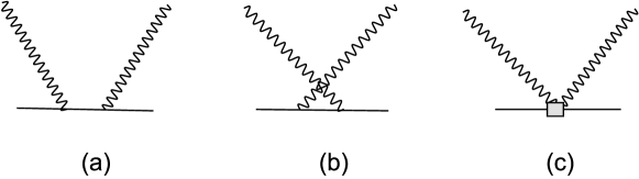
The polarizabilities arise in the context of low-energy structure of the nucleon. In the process of Compton scattering off the proton $\gamma p\to\gamma p$ they enter as coefficients in the low-energy expansion of the scattering amplitude. The Feynman diagrams of the process are shown in Fig. 2.

Figure 2: Feynman diagrams of low-energy Compton scattering off the nucleon

Here graphs 2a and  2b are the Born contributions, assuming that nucleon is a structureless object with mass, electric charge and anomalous magnetic moment. Graph 2c is the non Born contribution, and its leading order terms depend on 2 scalar and 4 spin polarizabilities.

Indeed, the scalar polarizabilities starts to contribute at second order in photon energy expansion of the amplitude yielding the following effective Hamiltonian:

$$H_{eff}^{(2)}=-4\pi\Big{[}\frac{1}{2}\alpha_{E1}\vec{E}^{2}+\frac{1}{2}\beta_{M1}\vec{H}^{2}\Big{]},$$ (4)

where $\vec{E}$ and $\vec{H}$ are the electric and magnetic dipole fields.

In order to introduce scalar polarizabilities in a Lorentz-invariant fashion, we write down an effective Lagrangian that yields the right Hamiltonian in the static limit, i.e.,

$${\mathcal{L}}_{NN\gamma\gamma} = \frac{2\pi}{M^{2}}(\partial_{\alpha}\overline{N})(\partial_{\beta}N)(\alpha_{E1}F^{\alpha\rho}F_{\rho}^{\beta}+\beta_{M1}\widetilde{F}^{\alpha\rho}\widetilde{F}_{\rho}^{\beta})$$ (5)

where $F_{\mu\nu}=\partial_{[\mu}A_{\nu]}$ is the electromagnetic field-strength tensor, $\widetilde{F}_{\mu\nu}=\epsilon_{\mu\nu\rho\sigma}\partial^{\rho}A^{\sigma}$, $N(x)$ is the nucleon Dirac-spinor field. Recalling that $\widetilde{F}^{\alpha\rho}\widetilde{F}_{\,\,\,\,\,\rho}^{\beta}=F^{\alpha\rho}F_{\,\,\,\,\,\rho}^{\beta}+\frac{1}{2}\eta^{\alpha\beta}F^{2}$, $F^{2}=-2(F^{0i})^{2}+(F^{ij})^{2}=-2{\bf E}^{2}+2{\bf B}^{2}$, and assuming the nucleon rest frame: $\partial_{i}N=0$, $\partial_{0}N=-iMN$, $\partial_{0}\overline{N}=iM\overline{N}$ we obtain

$${\mathcal{L}}_{NN\gamma\gamma} = 2\pi\left\{\beta_{M1}({\bf B}^{2}-{\bf E}^{2})+(\alpha_{E1}+\beta_{M1})\,{\bf E}^{2}\right\}\overline{N}N,$$

which readily reproduces the well known nonrelativistic Hamiltonian: $4\pi(-\mbox{\small{$\frac{1}{2}$}}\alpha_{E1}{\bf E}^{2}-\mbox{\small{$\frac{1}{2}$}}\beta_{M1}{\bf B}^{2})$.

The Lagrangian in Eq. (5) can also be rewritten as

$${\mathcal{L}}_{NN\gamma\gamma} = \pi\beta_{M1}\overline{N}NF^{2}\,$$

$$- \,\frac{2\pi(\alpha_{E1}+\beta_{M1})}{M^{2}}(\partial_{\alpha}\overline{N})(\partial_{\beta}N)F^{\alpha\mu}F^{\beta\nu}\eta_{\mu\nu}$$

which yields the following Feynman amplitude

$${\cal M}_{\mathrm{NB}}^{\mu\nu}\epsilon_{\mu}^{\prime}\epsilon_{\nu} = 4\pi\,\overline{u}(p^{\prime})\,u(p)\big{[}\beta_{M1}(q\cdot q^{\prime}\,\epsilon^{\prime}\cdot\epsilon-q\cdot\epsilon^{\prime}\,q^{\prime}\cdot\epsilon)$$ (7)

$$- \frac{\alpha_{E1}+\beta_{M1}}{2M^{2}}(p_{\alpha}^{\prime}p_{\beta}+p_{\alpha}p_{\beta}^{\prime})\,(q^{\prime\alpha}\epsilon^{\prime\mu}-q^{\prime\mu}\epsilon^{\prime\alpha})(q^{\beta}\epsilon_{\mu}-q_{\mu}\epsilon^{\beta})\big{]}$$

$$= \overline{u}(p^{\prime})\,u(p)\left[-A_{1}^{(\mathrm{NB})}(s,t)\,\mathscr{E}^{\prime}\cdot\mathscr{E}+A_{2}^{(\mathrm{NB})}(s,t)\,q\cdot\mathscr{E}^{\prime}\,q^{\prime}\cdot\mathscr{E}\right],$$

where $p$ and $q$ ($p^{\prime}$ and $q^{\prime}$) are the four-momenta of incident (outgoing) nucleon and photon, and the manifestly gauge-invariant polarization vectors are

$$\mathscr{E}_{\mu}=\epsilon_{\mu}-\frac{(p^{\prime}+p)\cdot\epsilon}{(p^{\prime}+p)\cdot q}\,q_{\mu}\,,\quad\quad\mathscr{E}_{\mu}^{\prime}=\epsilon_{\mu}^{\prime}-\frac{(p^{\prime}+p)\cdot\epsilon^{\prime}}{(p^{\prime}+p)\cdot q}\,q_{\mu}^{\prime}\,.$$ (8)

The polarizability contribution to the invariant Compton amplitudes is thus given as follows:

$$A_{1}^{(\mathrm{NB})}(s,t) = 2\pi(\alpha_{E1}+\beta_{M1})(\nu^{2}+\nu^{\prime 2})+2\pi\beta_{M1}t\,,$$ (9a)

$$A_{2}^{(\mathrm{NB})}(s,t) = -4\pi\beta_{M1}-\pi(\alpha_{E1}+\beta_{M1})\,t/(2M^{2}).$$ (9b)

We note that the contribution of $\alpha_{E1}+\beta_{M1}$ differs from conventional definitions by terms of higher order in the Mandelstam variable $t$, and, hence in energy. For instance, the difference of the present $A_{1}^{\mathrm{(NB)}}$ with the one in Ref. [1] is equal to $-(\pi/M^{2})(\alpha_{E1}+\beta_{M1})\,t(\omega^{2}-\mbox{\small{$\frac{1}{4}$}}t)$.

The last ingredient one needs to obtain the cross section is the proportionality factor between the matrix element squared and the cross section:

$$\frac{4\pi\alpha^{2}}{(s-M^{2})^{2}}dt.$$ (10)

This factor can also be expressed in terms of the solid angle $\Omega_{L}$ by using $dt=(\nu^{\prime 2}/\pi)d\Omega_{L}$, where $\nu^{\prime}$ is the outgoing photon energy.

The previous measurements of the scalar polarizabilities of nucleons were done in unpolarized Compton scattering experiments. The non-Born (NB) part of the unpolarized differential cross section for Compton scattering off a target with mass $M$ and charge $Ze$ is given by [8]:

$$\frac{d\sigma^{\mathrm{(NB)}}}{d\Omega_{L}} = -\frac{Z^{2}\alpha_{em}}{M}\left(\frac{\nu^{\prime}}{\nu}\right)^{2}\nu\nu^{\prime}\big{[}\alpha_{E1}\left(1+\cos^{2}\theta_{L}\right)$$ (11)

$$+ 2\beta_{M1}\cos\theta_{L}\big{]}+O(\nu^{4}),$$

where $\nu=(s-M^{2})/2M$ and $\nu^{\prime}=(-u+M^{2})/2M$ are, respectively, the energies of the incident and scattered photon in the laboratory frame, $\theta_{L}$ ($d\Omega_{L}=2\pi\sin\theta_{L}d\theta_{L}$) is the scattering (solid) angle; $s$, $u$, and $t=2M(\nu^{\prime}-\nu)$ are the Mandelstam variables; and $\alpha_{em}=e^{2}/4\pi$ is the fine-structure constant. Hence, given the exactly known Born contribution [9] and the experimental angular distribution at very low energy, one could in principle extract the polarizabilities with a negligible model dependence. In reality, however, in order to resolve the small polarizability effect in the tiny Compton cross sections, most of the measurements are done at energies exceeding 100 MeV, i.e., not small compared to the pion mass $m_{\pi}$. It is $m_{\pi}$, the onset of the pion-production branch cut, that severely limits the applicability of a polynomial expansion in energy such as LEX. At the energies around the pion-production threshold one obtains a very substantial sensitivity to polarizabilities but needs to resort to a model-dependent approach in order to extract them (see [6, 10] for reviews).

The magnetic polarizability $\beta_{M1}$ seems to be affected the most: the central value of the baryon chiral perturbation theory (BChPT) calculation is a factor of 1.5 larger than the PDG value. This is attributed to the dominance of $\alpha_{E1}$ in the unpolarized cross section. Thus it is desirable to find an observable sensitive to $\beta_{M1}$ alone, such that the latter could be determined independently of $\alpha_{E1}$.

Having this in mind, we found that the beam asymmetry could be such an observable. It is defined as

$$\Sigma_{3}\equiv\frac{d\sigma_{||}-d\sigma_{\perp}}{d\sigma_{||}+d\sigma_{\perp}},$$ (12)

where $d\sigma_{||}$ and $d\sigma_{\perp}$ are cross sections for photons polarized parallel and perpendicular to the scattering plane respectively.

Applying the LEX for the beam asymmetry we arrive at the following result for the proton ($Z=1$):

$$\Sigma_{3}=\Sigma_{3}^{(\mathrm{B})}-\frac{4M\omega^{2}\cos\theta\sin^{2}\theta}{\alpha_{em}(1+\cos^{2}\theta)^{2}}\,\beta_{M1}+O(\omega^{4}),$$ (13)

where $\Sigma_{3}^{(\mathrm{B})}$ is the exact Born contribution, while

$$\omega = \frac{s-M^{2}+\mbox{\small{$\frac{1}{2}$}}t}{\sqrt{4M^{2}-t}},\quad\theta=\arccos\left(1+\frac{t}{2\omega^{2}}\right)$$ (14)

are the photon energy and scattering angle in the Breit (brick-wall) reference frame. In fact, to this order in the LEX the formula is valid for $\omega$ and $\theta$ being the energy and angle in the laboratory or center-of-mass frame.

Equation (13) shows that the leading (in LEX) effect of the electric polarizability cancels out, while the magnetic polarizability remains. Hence, our first claim is that a low-energy measurement of $\Sigma_{3}$ can in principle be used to extract $\beta_{M1}$ independently of $\alpha_{E1}$.

However, the low-energy Compton experiments on the proton are difficult because of small cross sections and overwhelming QED backgrounds. Precision measurement only becomes feasible for photon-beam energies above 60 MeV and scattering angles greater than 40 degrees. Thus the experiments at MAMI are being carried at photon energies between 80 and 150 MeV. Since at these energies the effect of higher-order terms may become substantial one has to check the applicability of the leading LEX result. One way to do that is to compare the LEX result with the dispersion-relation calculations or calculations based on chiral perturbation theory.

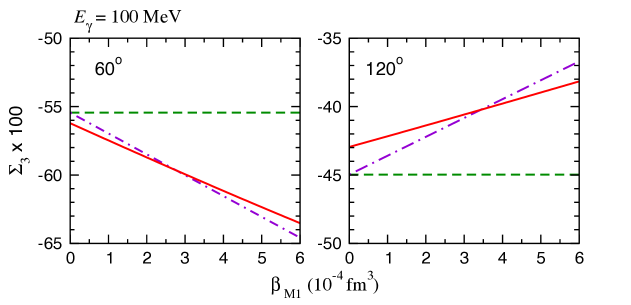
Figure 3: Beam asymmetry $\Sigma_{3}$ shown as function of $\beta_{M1}$ for fixed photon energy of 100 MeV and scattering angles of 60 (left panels) and 120 (right panels) degrees. The curves are as follows: dashed green — Born contribution; dash-dotted magenta — the leading LEX formula Eq. (13); red solid — NNLO BChPT [11].

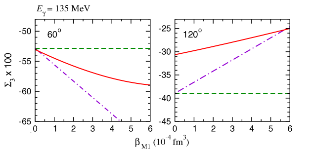
Figure 4: The same as in the previous figure but for photon beam energy of 135 MeV.

Figures 3 and 4 demonstrate such a comparison of the leading-LEX result to the next-next-to-leading order (NNLO) BChPT result of Ref. [11] for the beam asymmetry defined in Eq. (12). The observable is plotted for the case of proton Compton scattering as a function of magnetic polarizability of the proton. From Fig. 3 one sees that for the beam energy of 100 MeV the LEX is in a good agreement with the BChPT result, especially for the forward directions (left panels).

As expected we observe a significant sensitivity of $\Sigma_{3}$ to $\beta_{M1}$. Also, Fig. 3 shows that the beam asymmetry is large and, given the fact that many systematic errors tend to cancel out in this observable, the required accuracy to discriminate between the PDG and ChPT values for the magnetic polarizability should be much easier to achieve. Still, very high-intensity photon beams would be required to achieve the statistics necessary to pin down the magnetic polarizability model-independently to the accuracy currently claimed by the PDG, c.f. Eq. (1b). The high-intensity electron facility MESA being constructed in Mainz is very promising in this respect.

The results for the beam energy of 135 MeV (Fig. 4) show that the leading LEX result does not apply at such energies.

We next turn to the spin structure of the nucleon. It starts to show up at third order in photon energy in the expansion of Compton amplitude, yielding the following effective Hamiltonian [7]:

$$H_{eff}^{(3)}=-4\pi\Big{[}\frac{1}{2}\gamma_{E1E1}\vec{\sigma}\cdot(\vec{E}\times\dot{\vec{E}})+\frac{1}{2}\gamma_{M1M1}\vec{\sigma}\cdot(\vec{H}\times\dot{\vec{H}})$$ (15)

$$-\gamma_{M1E2}E_{ij}\sigma_{i}H_{j}+\gamma_{E1M2}H_{ij}\sigma_{i}E_{j}\Big{]},$$

here $\dot{\vec{E}}=\partial_{t}{\vec{E}}$,   $\dot{\vec{H}}=\partial_{t}{\vec{H}}$,   $E_{ij}=\frac{1}{2}(\nabla_{i}E_{j}+\nabla_{j}E_{i})$,   $H_{ij}=\frac{1}{2}(\nabla_{i}H_{j}+\nabla_{j}H_{i})$. Four constants $\gamma_{E1E1},\,\gamma_{M1M1},\,\gamma_{E1M2}$ and $\gamma_{M1E2}$ denote the spin polarizabilities.

Their contribution to the third order can be seen explicitly in the matrix-element in the Breit frame, that is given by

$$T_{\sigma^{\prime}\lambda^{\prime},\sigma\lambda} = \boldsymbol{\epsilon}^{\prime}\cdot\boldsymbol{\epsilon}\,A_{1}(\omega,\theta)+\boldsymbol{\epsilon}^{\prime}\cdot\hat{\mathbf{q}}\,\boldsymbol{\epsilon}^{\prime}\cdot\hat{\mathbf{q}}^{\prime}\,A_{2}(\omega,\theta)$$

$$+ i\boldsymbol{\sigma}\cdot(\boldsymbol{\epsilon}^{\prime}\times\boldsymbol{\epsilon})\,A_{3}(\omega,\theta)+i\boldsymbol{\sigma}\cdot(\hat{\mathbf{q}}^{\prime}\times\hat{\mathbf{q}})\,\boldsymbol{\epsilon}^{\prime}\cdot\boldsymbol{\epsilon}\,A_{4}(\omega,\theta)$$

$$+ [i\boldsymbol{\sigma}\cdot(\boldsymbol{\epsilon}^{\prime}\times\hat{\mathbf{q}})\,\boldsymbol{\epsilon}\cdot\hat{\mathbf{q}}^{\prime}-i\boldsymbol{\sigma}\cdot(\boldsymbol{\epsilon}\times\hat{\mathbf{q}}^{\prime})\,\boldsymbol{\epsilon}^{\prime}\cdot\hat{\mathbf{q}}]\,A_{5}(\omega,\theta)$$

$$+ [i\boldsymbol{\sigma}\cdot(\boldsymbol{\epsilon}^{\prime}\times\hat{\mathbf{q}}^{\prime})\,\boldsymbol{\epsilon}\cdot\hat{\mathbf{q}}^{\prime}-i\boldsymbol{\sigma}\cdot(\boldsymbol{\epsilon}\times\hat{\mathbf{q}})\,\boldsymbol{\epsilon}^{\prime}\cdot\hat{\mathbf{q}}]\,A_{6}(\omega,\theta)$$

where $\mathbf{q}$ and $\boldsymbol{\epsilon}$ ($\mathbf{q}^{\prime}$ and $\boldsymbol{\epsilon}^{\prime}$) are momentum and polarization vector of the incoming (outgoing) photon, hats indicate unit vectors, $\omega$ and $\theta$ are its energy and scattering angle in the Breit frame; $A_{1}-A_{6}$ functions are invariant amplitudes with the LEX expansion given by

$$A_{1} = -Z^{2}+\frac{1}{4}\left[(Z+\kappa)^{2}(1+z)-Z^{2}\right](1-z)\,\omega^{2}+4\pi(\alpha_{E1}+\beta_{M1}z)\,\omega^{2}+O(\omega^{4}),$$

$$A_{2} = \frac{1}{4}\kappa\,z(2Z+\kappa)\,\omega^{2}-4\pi\beta_{M1}\omega^{2}+O(\omega^{4}),$$

$$A_{3} = \frac{1}{2}\left[Z(Z+2\kappa)-(Z+\kappa)^{2}\,z\right]\,\omega-4\pi\,\omega^{3}\left[\gamma_{\text{E1E1}}+\gamma_{\text{E1M2}}+z\left(\gamma_{\text{M1E2}}+\gamma_{\text{M1M1}}\right)\right]+O(\omega^{4}),$$

$$A_{4} = -\frac{1}{2}(Z+\kappa)^{2}\,\omega-4\pi\,\omega^{3}\left(\gamma_{\text{M1M1}}-\gamma_{\text{M1E2}}\right)+O(\omega^{4}),$$

$$A_{5} = \frac{1}{2}(Z+\kappa)^{2}\,\omega+4\pi\,\omega^{3}\,\gamma_{\text{M1M1}}+O(\omega^{4}),$$

$$A_{6} = -\frac{1}{2}Z(Z+\kappa)\,\omega+4\pi\,\omega^{3}\,\gamma_{\text{E1M2}}+O(\omega^{4}).$$ (17)

Here $z=\cos\theta$, $Ze$ and $\kappa$ are the charge and anomalous magnetic moment of the nucleon.

Knowledge of the helicity amplitudes of Eq. (Proton polarizabilities from polarized Compton scattering: low-energy expansion) allows one to construct various observables and study their sensitivity to spin polarizabilities. Two observables turn out to be of particular interest for determination of spin polarizabilities: the beam target asymmetries with circularly-polarized photons and longitudinally (transversely) polarized target, i.e. $\Sigma_{2z}$ ($\Sigma_{2x}$). Applying the LEX for the beam-target asymmetries, we obtain that the leading non-Born terms in the Breit frame are:

$$\Sigma_{2x}-\Sigma_{2x}^{\mathrm{(B)}} = \frac{\sin\theta\,\omega^{3}}{\left(1+z^{2}\right)\alpha_{em}}\{\alpha_{E1}[(1+\kappa)^{2}-(1+2\kappa)z]$$

$$+ \frac{\beta_{M1}}{1+z^{2}}[\kappa+3(1+\kappa)^{2}z-3(1+2\kappa)z^{2}-(1+\kappa)^{2}z^{3}+(1+\kappa)z^{4}]$$

$$+ 2\left[\gamma_{M1M1}+z\left(\gamma_{E1E1}+\gamma_{E1M2}\right)+z^{2}\,\gamma_{M1E2}\right]\},$$

$$\Sigma_{2z}-\Sigma_{2z}^{\mathrm{(B)}} = \frac{\,\omega^{3}}{(1+z^{2})\alpha_{em}}\{\alpha_{E1}[-\kappa+2(1+\kappa)^{2}z-(2+3\kappa)z^{2}]$$ (18b)

$$+ \frac{\beta_{M1}}{1+z^{2}}[-(1+\kappa)^{2}+(1-\kappa)z+6(1+\kappa)^{2}z^{2}-2(3+4\kappa)z^{3}-(1+\kappa)^{2}z^{4}+(1+\kappa)z^{5}]$$

$$+ 2[(1+z^{2})(\gamma_{E1E1}+z\,\gamma_{M1E2})+2z(\gamma_{M1M1}+z\,\gamma_{E1M2})]\}.$$

Unfortunately, the applicability of Eq. (18) is very limited.

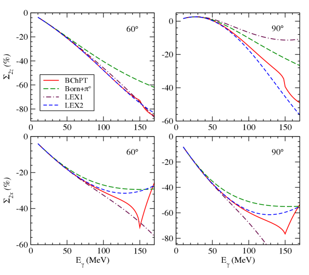
Figure 5: The beam-target asymmetries $\Sigma_{2z}$ (upper panel) and $\Sigma_{2x}$ (lower panel) as a function of incident photon energy for scattering angle of 60 (left panel) and 90 (right panel) degrees. The curves are as follows: dashed green — Born contribution; red solid — NNLO BChPT; dashed blue — the LEX with only invariant amplitudes expanded; dash-dotted magenta — the leading LEX formulas Eqs. (18) with both the invariant amplitudes and helicity amplitudes expanded.

Similarly to the case of the LEX for the beam asymmetry, we define it by comparing the leading order LEX results of Eq. (18) with results obtained in BChPT. Figure 5 demonstrates such a comparison. Two LEX curves correspond to the expansion of the invariant amplitudes (LEX2 curve) and additionally the expansion of the helicity amplitudes (LEX1 curve given by Eq. (18)). One sees that LEX and BChPT curves coincide only for photon energy below 50 MeV, thereby defining the region of applicability. However, at these low energies (below 50 MeV), one finds the leading order LEX in Eq. (18) to be suppressed by $\omega^{3}$. The sensitivity to spin polarizabilities becomes too small to allow one to extract them from current experiments. Therefore, the spin polarizabilities are planned to be extracted at higher energies (around the Delta resonance region), where the sensitivity of the observables becomes significant. As discussed above, the LEX approach fails, and one has to resort to either dispersion relations or ChPT approach.

To conclude, we claim that the beam asymmetry $\Sigma_{3}$ should be used for accurate determination of the magnetic polarizability $\beta_{M1}$ from low-energy Compton scattering. While the cross sections receive contributions from both the electric and magnetic polarizability, the effect of $\alpha_{E1}$ cancels out from the asymmetry at leading order in the low-energy expansion. We have also studied the next-to-leading corrections and found them to be suppressed at the forward scattering angles [5]. A precise and model-independent determination of the proton $\beta_{M1}$ is feasible through a precision measurement of $\Sigma_{3}$ at beam energies below 100 MeV and forward scattering angles. Furthermore, when multiplied with the unpolarized cross section, $\Sigma_{3}$ yields the polarized cross section difference, which provides an exclusive access to the electric polarizability.

Besides the scalar polarizabilities, we have studied observables sensitive to spin polarizabilities. The problem here is the small region of applicability of the LEX results, i.e. photon energy below 50 MeV. At such energies the sensitivity of LEX results to spin polarizabilities becomes too small to discriminate their effect from the Born contribution. In this case, one has to resort to either ChPT or dispersion relation approaches. Both work at higher energy regimes, and the fact that sensitivity to spin polarizabilities increases increasing the energy, suggests an idea to extract them around the Delta resonance region, where the sensitivity becomes substantial. Nevertheless, we obtained the LEX expressions for the non-Born leading order terms of beam-target asymmetries $\Sigma_{2z}$ and $\Sigma_{2x}$, cf. Eq. (18). Although one cannot use these expressions for determination of the spin polarizabilities, they could provide a low energy test for either the ChPT or dispersion relation frameworks.

I would like to thank Vladimir Pascalutsa for advising me during this work, and to acknowledge the support of the Graduate School DFG/GRK 1581 “Symmetry Breaking in Fundamental Interactions”.