Longitudinal top polarisation measurement and anomalous coupling
Abstract
Kinematical distributions of decay products of the top quark carry information on the polarisation of the top as well as on any possible new physics in the decay of the top quark. We construct observables in the form of asymmetries in the kinematical distributions to probe their effects. Charged-lepton angular distributions in the decay are insensitive to anomalous couplings to leading order. Hence these can be a robust probe of top polarisation. However, these are difficult to measure in the case of highly boosted top quarks as compared to energy distributions of decay products. These are then sensitive, in general, to both top polarisation and top anomalous couplings. We compare various asymmetries for their sensitivities to the longitudinal polarisation of the top quark as well as to possible new physics in the vertex, paying special attention to the case of highly boosted top quarks. We perform a - analysis to determine the regions in the longitudinal polarisation of the top quark and the couplings of the vertex constrained by different combinations of the asymmetries. Moreover, we find that use of observables sensitive to the longitudinal top polarisation can add to the sensitivity to which the vertex can be probed.
I Introduction
The top quark is the heaviest of all fundamental particles discovered so far in the Standard Model(SM). Since the mass of the top quark ( ) Beringer et al. (2012) is very close to the electroweak symmetry breaking (EWSB) scale, effects of any New Physics (NP) associated with EWSB are likely to reveal themselves in the properties of the top quark. The LHC, during the course of its runs, is expected to determine several of the properties of the top quark Beneke et al. (2000); *Han:2008xb; *Bernreuther:2008ju; *Schilling:2012dx; *BARBERIS:2013wba; *JABEEN:2013mva. A comparison of these with expectations from the SM will reveal NP, if present. In the search for NP, there are already some results from the LHC, which include those on the top-quark polarisation and anomalous couplings in the vertex Aad et al. (2013a); CMS (2012), which are relevant to the discussion in this paper.
New Physics may appear in the production of the top quark or its decay or both [seeforexample]Cheung:1995nt; *PhysRevD.54.4326; *PhysRevD.61.119901; *Godbole:2002qu; *Choudhury:2009wd; *Gupta:2009wu; *HIOKI:2011xx; *Choudhury:2012np; Antipin and Valencia (2009); Bernreuther and Si (2013). A model-independent way of probing NP in the top sector is provided by the effective-theory formalism where all gauge-invariant higher-dimensional operators suppressed by powers of the corresponding scale of NP are added to the SM Lagrangian (Buchmuller and Wyler (1986); *Grzadkowski:2003tf; *Grzadkowski:2010es; Aguilar-Saavedra (2009); Bach and Ohl (2012); Zhang and Willenbrock (2011)). This description is valid at scales much lower than the NP scale. A complete set of dimension-six operators relevant to top production and decay can be found in Zhang and Willenbrock (2011). Higher order effects within the SM itself could induce structures that are not present at the tree level vertex (see for example, Fischer et al. (2002); Czarnecki (1990); *Li:1990qf; Gonzalez-Sprinberg et al. (2011)).
The top quark, on account of its large mass, decays before it hadronises, thereby transferring its spin information to the decay products. The angular and energy distributions of the decay products carry information on the spin of the top quark Jezabek and Kuhn (1989a); Czarnecki et al. (1991); Kane et al. (1992a); Bernreuther et al. (1992); *Erratum. Kinematic distributions of the decay products of the top in the presence of anomalous couplings have been studied, without assuming any model, in Jezabek and Kuhn (1994); Nelson et al. (1997); Godbole et al. (2006); Rindani (2000). Effects of higher order QCD corrections on the distibutions are studied in Jezabek and Kuhn (1989a); Czarnecki et al. (1991); Jezabek and Kuhn (1989b); Fischer et al. (2002); Brandenburg et al. (2002); Bernreuther et al. (2004); Groote et al. (2007); Hagiwara et al. (2007); Kitadono and Li (2013); Brucherseifer et al. (2013); Bernreuther et al. (2014).
The polarisation of top quarks produced in a hadron collider like the LHC depends upon the hard subprocesses that produce them. Since QCD which is mainly responsible for top-pair production in the SM is a vector interaction, there is no significant longitudinal polarisation of the top quarks pair produced in the SM: less than about a percent, after taking into account the one loop electro weak radiative corrections, in the so-called helicity basis111Helicity basis is defined as the basis in which the top spin quantisation axis is taken along the direction of motion of the top. defined in centre of mass (c.m) frame of collisions at the LHC Bernreuther et al. (2006); *Bernreuther:2008md; Kuhn et al. (2007); *PhysRevD.91.014020. Single-top production, occurring via electro-weak interactions at much lower rates, does give rise to polarised top quarksMahlon and Parke (2000); Schwienhorst et al. (2011). The value of polarisation after including NLO QCD corrections is 0.91 in the helicity basis defined in the c.m frame of the top quark and the spectator jet (the jet from the light quark that is scattered away along with the top) Schwienhorst et al. (2011). Note that the top can be polarised along a direction that is perpendicular to the plane of production of the top (‘transverse polarisation’). While in the SM longitudinal polarisation requires parity violating interactions, transverse polarisation is allowed even when the interactions are parity conserving as in the case of QCD. This however, is generated only at one loop level in QCD. In the case of top pair production, it does not exceed at the parton level Dharmaratna and Goldstein (1990); *PhysRevD.45.124; Bernreuther et al. (1996). This value is further reduced at the LHC due to the dominance of the gluon fusion channel in production: at 7 TeV Baumgart and Tweedie (2013). In this work, we focus only on the longitudinal polarisation. Hence, in our paper the term top polarisation always refers to the longitudinal polarisation unless it is explicitly stated otherwise.
Since the standard model value of top polarisation in top pair production is small, an observation of substantial polarisation in top-pair production will strongly indicate NP. Any nontrivial chiral structure in the top coupling induced by the NP can affect the polarisation of the produced top quarks Nojiri (1995); *Perelstein:2008zt; *Arai:2010ci; Gopalakrishna et al. (2010); *Godbole:2010kr; Huitu et al. (2011); *Rindani:2011pk; *Biswal:2012dr; *Belanger:2012tm; *Belanger:2013gha; *Taghavi:2013wy; *Aguilar-Saavedra:2014eqa; Bernreuther and Si (2013).Hence measurement of the polarisation of the top quark can provide information on the chiral structure of the couplings involved in NP contributions to top quark-production Nojiri (1995); *Perelstein:2008zt; *Arai:2010ci; Gopalakrishna et al. (2010); *Godbole:2010kr; Huitu et al. (2011); *Rindani:2011pk; *Biswal:2012dr; *Belanger:2012tm; *Belanger:2013gha; *Taghavi:2013wy; Cao et al. (2011); *Choudhury:2010cd; *Krohn:2011tw; Falkowski et al. (2013); *Godbole:2011vw.
New physics reflects itself in changes in total and differential cross sections for top production. Detailed study of angular distributions of the decay products of the top quark, which are also affected by top-quark polarisation, provides a useful handle for discrimination between different NP models. Moreover, when NP couplings are small and the deviations of the total cross section from theoretical predictions in the SM can be small, the kinematic distributions and final-state polarisations being sensitive to the interference between the SM contribution and NP contribution can lead to increased sensitivity. The top-quark polarisation can, in addition, give a handle on the chiral structure of the couplings in NP.
A number of interesting scenarios for the production of top quarks occur once extensions of the standard model are introduced. The most popular extensions include supersymmetry, theories with extra dimensions and theories with extended gauge groups, all of which introduce new particles, which would contribute to top quark production in various ways: through an on shell production of resonances or via virtual effects. As said before, a nontrivial chiral structure of the top-quark couplings induced by the NP will lead to a prediction for top-quark polarisation which depends on the values of the parameters of that particular extension of the SM being considered.
Some of the NP models predict new heavy resonances with masses at the TeV scale Randall and Sundrum (1999); *Agashe:2004rs; *Agashe:2006hk. Such heavy resonances are produced effectively at rest in the parton centre-of-mass (cm) frame. When these heavy resonances decay into top quarks, the resulting top quarks are highly boosted in the lab frame. The decay products of these highly boosted top quarks are collimated along the direction of motion of the parent top quark. In such a case observables based on the energy distributions of the decay products rather than their angular distributions are more suitable to probe the polarisation of the top quark Shelton (2009). For such highly boosted tops methods based on jet substructure have been proposed to extract information on the polarisation of the top which then can be used to get information on the production mechanism of top quarks Krohn et al. (2010); *Bhattacherjee:2012ir; *Kitadono:2014hna. Recently a new method for measuring the polarization of top, when the top decays hadronically, has been proposed Tweedie (2014). This method, involving a weighted average, in the top rest frame, of the directions of two light-quark jets that come from the decay , has been shown to perform better than methods based on other hadronic top spin analysers.
Data from the LHC has placed stringent lower bounds on the masses of resonances Chatrchyan et al. (2012); *Chatrchyan:2012oaa; *Aad:2012em; *Aad:2012raa; *Aad:2013nca. If they do exist at higher masses, the observation in the invariant mass distribution would be difficult. On the other hand, NP production amplitude of the resonance giving rise to a top pair could have sizable interference with the SM amplitude. This could lead to observable top polarization provided the NP couplings have a nontrivial chiral structure. Top polarization can serve as a tool in testing these models Gopalakrishna et al. (2010); *Godbole:2010kr.
Another example of significant top polarisation is in stop decay
| (1) |
in the minimal supersymmetric standard model (MSSM), where is the lightest stop and , ,…,4 stand for the four neutralinos, which can be used to study mixing in the sfermion sector as well as the neutralino-chargino sector Perelstein and Weiler (2009); Low (2013); Belanger et al. (2013b, a). In -parity violating MSSM, top quarks pair produced via a -channel exchange of a stau or a stop or a top quark produced in association with a slepton, can have nonzero polarisation, whose measurement can be used to constrain the -parity violating couplings Hikasa et al. (1999); Nie et al. (2005); Arai et al. (2010). There have been several NP explanations of the forward-backward asymmetry of the top quark observed at Tevatron (see, for example Jung et al. (2010); *Frampton:2009rk; *Shu:2009xf; *Cao:2010zb; *Dorsner:2009mq; *Cheung:2009ch; *Djouadi:2009nb; *Arhrib:2009hu; Bai et al. (2011); *Gresham:2011pa; *Buckley:2011vc; *Bhattacherjee:2011nr; *AguilarSaavedra:2011vw; *AguilarSaavedra:2011ug; *Chivukula:2010fk; *Grinstein:2011yv; *Tavares:2011zg; *Jung:2011zv; *Ligeti:2011vt; Biswal et al. (2012); *Allanach:2012tc; *Dupuis:2012is; *Aguilar-Saavedra:2014yea; Baumgart and Tweedie (2013)), and top polarisation can be useful in discriminating among them Choudhury et al. (2011); Krohn et al. (2011); Cao et al. (2012); Fajfer et al. (2012). In fact the top polarisation transverse to the production plane also could be used to test whether the measured forward-backward asymmetry at the Tevatron is due to the effect of some NP in the top pair production Baumgart and Tweedie (2013), even when the NP is difficult to be observed directly.
Since the top quark mainly decays through the channel with a branching ratio of , any new physics which appears through the vertex can affect the measurement of polarisation of top quarks which is determined by the production process. In general, measures of top polarisation have a dependence both on the strength and the tensor structure of the coupling associated with top decay. Measures of top polarisation which depend only on the energy integrated angular distributions are insensitive to the anomalous part of the decay vertex Grzadkowski and Hioki (2000); *Grzadkowski:2001tq; *Grzadkowski:2002gt; Rindani (2000); Godbole et al. (2006). Recently another measure of top-quark polarisation has been proposed in Aguilar-Saavedra and Herrero-Hahn (2013) which factors out the the effect of any possible anomalous vertex from the polarization of the top quark. The factor which contains the information about the vertex of the top decay can be extracted in a model-independent way from the angular distributions of the top quark’s decay products Aguilar-Saavedra et al. (2007). Since the anomalous coupling also affects the kinematic distributions of the decay products of the top quark, it too can be probed by studying these and such probes have been constructed Boos et al. (1999); Águila and Aguilar-Saavedra (2003); Hubaut et al. (2005); Mohammadi Najafabadi (2007); Aguilar-Saavedra et al. (2007); Aguilar-Saavedra (2008); Najafabadi (2008); Aguilar-Saavedra et al. (2008); Aguilar-Saavedra and Bernabeu (2010); Rindani and Sharma (2011, 2012). Probing anomalous couplings at future colliders such as LHeC and ILC have also been considered by various authorsBoos et al. (2000); Dutta et al. (2013); Lin et al. (2002); Devetak et al. (2011).
Since the NP can affect top polarisation as well as give rise to anomalous decay vertex, it is of interest to explore how well one can study simultaneously both the top polarisation and the anomalous couplings and further see how probes of one are influenced by the other. We present in this note some observations on construction of various observables as a measure of top polarisation and how one can simultaneously probe top polarization and the anomalous coupling, when neither of the two is known a priori.
Studies of spin effects in top physics have largely concentrated on spin correlations in top pair production, as these are nonzero even in the SM and the measurements are interesting, even if no NP effects exist. A comparison of experimental results with SM predictions can then be used to constrain the NP models. The results so obtained at the Tevatron and the LHC have so far shown consistency with the SM, though errors are large. These correlations are best measured using leptonic final states from both top and anti-top. It is conceivable that a single polarisation measurement on either the top or the anti-top which decays leptonically, allowing the other to decay hadronically, could add to the accuracy.
Moreover, attempts to measure single-top polarisation at the Tevatron and at the LHC have so far been made by reconstructing the rest frame of the top quark. A method which does not require such full reconstruction of the top may be desirable. We have thus concentrated on the measures of the polarization of a single top in the laboratory frame.
We construct various kinematic observables (asymmetries), make a comparative study of their dependence on top polarisation and anomalous vertex, and examine the possibility of simultaneously constraining the anomalous vertex and the polarisation of the top quark. Our observables do not always require full reconstruction of the top momentum. We do not look at any specific top production mechanism, but simply consider the top quark to be produced in the lab frame with various momenta, paying special attention to highly boosted top quarks.
Our paper is divided into four sections. In section II we describe the structure of vertex and constraints on various anomalous couplings. In section III we make a comparative study of the sensitivities of different asymmetries to the polarisation of the top and anomalous couplings. In section IV we use these asymmetries to constrain simultaneously the polarisation of the top quark and the vertex. In section V we give a summary and conclusions. 222In this work all kinematic quantities in the rest frame of the top quark are denoted by a subscript ‘0’. All kinematic quantities which do not have subscript ‘0’ are in the laboratory frame (lab frame), unless stated otherwise. We have assumed that the top quark has spin along the direction of motion of the top in the lab frame. The lab frame polarisation is obtained from the rest frame one by a boost along the direction of motion of the top quark. We use the word lepton to denote the charged anti-lepton from .
II The structure of vertex
The vertex in the SM has a structure. Depending upon the NP the structure of vertex can be modified from the structure [see; forexample]Bernreuther:2008us. We follow a model-independent approach by writing down the most general vertex Aguilar-Saavedra et al. (2007):
| (2) |
where is the gauge coupling constant, are the four-momenta of the top and the bottom quarks respectively, and are the left and right chiral projectors. In the SM, and at tree level. One loop QCD contributions to the vertex have been computed within the SM, inCzarnecki (1990); *Li:1990qf; *Brandenburg:2002xr . Electroweak corrections also affect the vertex and in turn affect the couplings and . One loop EW contributions to the tensor couplings amount to about of the one loop QCD contributions Gonzalez-Sprinberg et al. (2011). After including the EW contributions the tensor couplings at one loop level in the SM are as follows: and Gonzalez-Sprinberg et al. (2011).
We take the CKM matrix element . Similarly, the vertex with anomalous couplings is given by
| (3) |
When CP is conserved, , , and Rindani and Sharma (2012). Direct searches of NP in top decay at the Tevatron give constraints on the coefficients: , , at 95 % C.L assuming Abazov et al. (2012). Indirect constraints from the measurement of the branching ratio of are stronger for , and weaker for :, , Grzadkowski and Misiak (2008) at 95% C.L. Direct search constraints are given also by the LHC: for , the CMS collaboration CMS (2012) obtained as a best fit value of the tensor part of the coupling which in our notation reads as in a fit to measured helicity fractions proposed by Kane et al. (1992a). A combination of data from the Tevatron, and the LHC on observables like the -channel single top cross section, and the helicity fractions, gives, in our sign conventions, and respectively at 95 C.LBernardo et al. (2014). When CP is conserved, the constraints on the anomalous couplings , , and are the same as those for , , and respectively.
In the analytical expressions for different kinematic distributions (see below) we have assumed that the anomalous couplings and are real valued while all other anomalous couplings are complex valued. However, in view of the strong constraints on the anomalous couplings, in our numerical work and in analyical results on vertex, we set . In numerical works, we also set and take as a real valued quantity varying in the range to .
III Kinematic distributions of the decay products of the top
Recall that a measurement of the polarisation of the top quark can only be done through the kinematic distributions of its decay products and these would also be affected by the nature of the coupling.
We begin by looking at the details of the three-body decay of the top quark. The top quark decays into a quark and a boson which in turn decays into a charged anti-lepton () and a neutrino . We assume that all the particles in the decay chain are on-shell (including the intermediate boson). The angular distributions of the decay products are correlated to the polarisation of the top quark. In the SM, in the rest frame of the top quark, the energy integrated distribution is given by
| (4) |
where , the quantity is called the spin-analysing power of the particle and is the angle between the direction of the momentum of the particle and the top quark spin axis in the rest frame of the top quark. The spin-analyzing powers of the quark, lepton and the neutrino in the SM at tree level are
respectively, where Jezabek (1994). Higher order QCD effects on the spin analysing power of the lepton are at the per-mille level Czarnecki et al. (1991). But in the case of hadronic decay of the top, the QCD corrections to the spin analysing powers of quarks from the top decay can be upto about Brandenburg et al. (2002); Bernreuther et al. (2014).
III.1 Kinematics of the top decay
Before proceeding to the description of asymmetries, we give a brief description of the kinematics of the top quark decay: .
The conservation of energy and momentum and the on-shell condition of give the following equations:
| (5) |
and
| (6) |
where are the four-momenta of the particles. Solving these equations along with the on-shell condition of the particles fixes all but four variables in the rest frame of the top quark: energy of the lepton , the polar and azimuthal angles of the lepton and the azimuthal angle () of the quark with respect to a coordinate system where the azis is along the direction of the lepton momentum. The variables fixed by eqs. 5 and 6 and the on-shell conditions are, the energy of the quark, and the cosine of the angle between the -quark momentum and the lepton momentum, where, . The energy of the lepton is constrained to vary between and .
III.2 Definition of asymmetry
Asymmetry in a kinematic variable is defined (in a given frame) as
| (7) |
where is the differential partial decay width of the top quark in the variable and is a value of between chosen as a reference point about which the asymmetry is evaluated. In this work, we chose reference points on the basis of the following considerations:
-
1.
The reference point should be such that the evaluated asymmetry is sensitive to both of the parameters and throughout their allowed range of values. In other words, the asymmetries thus obtained should be able to distinguish between different values of the parameters.
-
2.
The choice of the reference point should allow for a comparison of cases of different values of the parameters.
The asymmetries vary in their sensitivity to the polarisation of the top quark and the anomalous coupling , and in their usefulness in a particular kinematic regime of top decay. We describe four such asymmetries in this section. We can classify them into broadly two categories: angular asymmetries and energy-based asymmetries. Examples of the former include and of the latter include , , and . When the top quarks are highly boosted, the decay products of the top are highly collimated. In this case measurement of angular distribution of visible decay products is possible but difficult ATL (2010). Hence energy-based asymmetries are used to probe the top-quark polarisation Shelton (2009) and vertex.
III.3 The asymmetry ()
The asymmetry is defined in terms of where is the angle between the momentum of the lepton from the decay and the top quark direction of motion. The distribution is sensitive to the polarisation of the top quark (). In the rest frame of the top quark the distribution is given in the SM by
| (8) |
This expression is valid even when the anomalous coupling is non zero provided it is small Grzadkowski and Hioki (2000); *Grzadkowski:2001tq; *Grzadkowski:2002gt; Rindani (2000); Godbole et al. (2006). In the lab frame the distribution becomes Rindani and Sharma (2011)
| (9) | ||||
where is the cosine of the angle between the top quark direction of motion and the lepton momentum in the lab frame. In eq. 9, the factor in the denominator of the right-hand side is given by
| (10) |
and is the boost required to go from the lab frame to the top-quark rest frame. When , keeping only terms which are first order in , we get
| (11) |
which is completely independent of the anomalous coupling . In other words, the energy-integrated distribution is only very very weakly dependent on the anomalous coupling .
Therefore the lepton angular asymmetry () serves as a useful measure of polarisation of the top quark irrespective of NP effects at the decay vertex when they are small Godbole et al. (2006).
In the SM, the asymmetry about the point is given in the lab frame, using eq. 7, by
| (12) |
From this equation one can easily observe that the sensitivity of to the polarisation of the top quarks decreases with increasing boost. This can be understood as follows: In the rest frame of the top quark, the lepton is preferentially emitted either in the forward direction or the backward direction depending upon the sign of the polarisation of the top quark () (eq. 8). But in the lab frame, at large values of boost, the lepton emission is strongly suppressed except in the direction due to kinematics which appears through the factor in eq. 9 for all values of polarisation . This means that the lepton angular distribution loses its sensitivity to at large boosts as shown in eq. 12.
III.4 The asymmetry ()
The variable is defined as where is the energy of the lepton from the top decay in a given frame. Unlike the distribution, the distribution is not insensitive to in the top quark rest frame. The analytical expression for the distribution , in the top quark rest frame, is given by
| (13) | ||||
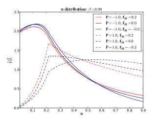
where is given in eq. 10. In the case when the distribution is not independent of as the factors that are linear in do not cancel each other from the denominator and the numerator of eq. 13. The distribution is plotted in fig. 1 for different values of the top polarisation and the anomalous coupling . The location of the peak of the distribution for a given top polarisation depends upon the anomalous coupling as can be seen from the figure. The sharp edges in the distribution for appear due to the interplay of the polarisation of the top and the kinematics of the top decay.
It would be convenient if the value of at the position of the peak is chosen as the reference point to evaluate the asymmetry . In view of the fact that this point varies with as well as , for uniformity we take the value of corresponding to the peak of the distribution for and as a reference point for all values of and . This choice is consistent with our method of choosing the reference points as given in Sec. III.2.

The above equation also shows that the distribution is independent of in the rest frame of the top quark. Therefore the asymmetry has no sensitivity to the polarisation of the top quark () in the top quark rest frame. But under a Lorentz transformation along the top quark direction of motion which takes the top quark rest frame to the lab frame, the energy of the lepton in the lab frame gets related to both the energy and the polar angle of the lepton measured in the top quark rest frame:
Since the distribution in is correlated to the top quark polarisation () (see eq. 8) , the distribution in (or ) becomes dependent on . Hence the asymmetry for depends on the polarisation of the top quark ().
A variable similar to has been proposed in Berger et al. (2012). It is defined as and it is related to by a boost dependent factor: . However, the asymmetry constructed out of - distribution is the same as the asymmetry at any given value of .
III.5 The Asymmetry ()
The variable is defined as where and are the energies in the lab frame carried by the lepton and the quark respectively Shelton (2009). The variable can be written as
| (14) |
where , and are the energy and the angle between the top quark direction of motion and the momentum of the lepton measured in the top quark rest frame respectively. is given by
| (15) |
with and ,. varies in the range . The distribution is given by
| (16) |
where is as defined in eq. 10, and , are the roots of the equation .
Since is invariant under the transformation , we have two solutions: and with . The function is given by
| (17) |
where
| (18) |
This equation determines which can be used to get the value of the distribution at . The asymmetry is calculated the point using eq. 7.
We note that the -distribution is independent of to linear order: the integrand of eq. 16 actually has an additional term that is proportional to . Since the -distribution is obtained after summing over two values of i.e and , this additional term does not give any contribution.
The distribution for different value of and is given in fig. 2. Similar to the case of distribution, the distribution has sharp edges due to the same reasons given in sec. III.4.
III.6 The asymmetry ()
The variable is defined as where and are the energies in the lab frame carried by the and quarks respectively Shelton (2009). The variable can be related to the variables defined in the rest frame of the top quark:
| (19) |
where is as defined in eq. 15. Since varies in the range , the variable varies in the range . The distribution is given by
| (20) |
The distribution is plotted in fig. 3 for different values of the top polarisation and the anomalous coupling . One can easily observe that the effect of the anomalous coupling is to change the slope of the distribution which will be explained below.
Since the distribution is linear in , an analytical expression for the asymmetry can be easily found. We take as the reference point , the value of which corresponds to i.e . To simplify the notation let us define two functions of : and . Then the distribution in can be rewritten in terms of (see Rindani and Sharma (2011); Aguilar-Saavedra and Bernabeu (2010)):
| (21) |
Now changing the variable from to we get the limits of the integration in eq. 7 as and . Only the term linear in survives in the numerator and the expression for is given by
| (22) |
Therefore the asymmetry is directly proportional to the top-quark polarisation and is independent of the boost factor as and are independent of both and . Moreover the distribution can be directly related to the angular distribution of the quark in the top rest frame due to eq. 19. In fact, substituting the relation eq. 19 in eq. 21, we get,
| (23) |
where is the spin-analysing power of the quark in the presence of anomalous coupling . It includes correction to the SM tree level value of . To second order in , can be written as
| (24) | ||||
Substituting the values of and Beringer et al. (2012), we get the numerical value of as
Since the coefficiets of and are much greater than the constant term in the above equation and the alternate terms differ in their signs, cancellation between different terms can occur. Therefore the effect of the anomalous coupling on the distribution is non-trivial. As an observable based on the ratio of the energy of the top quark decay products (in the lab frame), can be used along with to probe top-quark polarisation at large boosts.


III.7 CP violation in the top decay
Here we note that using the asymmetries constructed for the and decay, one can probe CP violation in the decay of top and anti-top assuming CP conservation in the production of top and anti-top quarks. As mentioned earlier, in the presence of CP conservation , , and . When the production process is CP-conserving, polarizations of the top () and the anti-top () are related: . In this limit, the difference in the -asymmetries of the top and the anti-top decay is proportional to to linear order in the anomalous couplings (see eq. 16). The coefficient of proportionality is a function of top polarization () and the boost . Here is set to unity, and to zero. Similarly, the difference in -asymmetries of the top and the anti-top is proportional to with a factor for and . Note that CP violation in decay necessarily requires an absorptive part in the amplitude and hence in any underlying theory it is expected that would be loop suppressed.
III.8 Sensitivity of the asymmetries to and
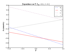
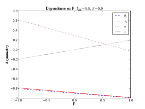
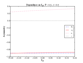
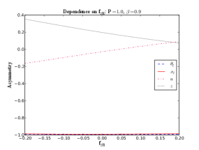
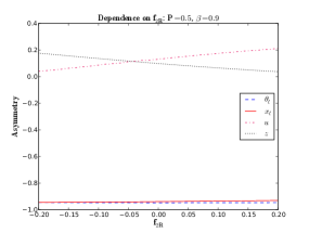
The dependences of various asymmetries on the polarisation of the top quark are compared in fig. 4. One can observe that for moderate values of boost all the four asymmetries are sensitive to the top polarisation while for large values of boost, and are more sensitive as compared to and . For very small values of boosts (), the angular asymmetry has the highest sensitivity to the top-quark polarisation () due the fact that the charged lepton has the maximal spin-analysing power. follows in the sensitivity to for as it is directly proportional to the spin-analysing power of the quark (). This is true as long as the value of the anomalous coupling does not reduce the value of . From equation eq. 24 or from the plots of in fig. 5, one can easily see that the value of monotonically increases with in the range . Therefore as a measure of top quark polarisation, is better for negative values of than for positive values. In a detailed comparison, for , turns out to be the second best in the sensitivity to , surpassed only by .
An additional result of the comparison is that the sensitivity of to is higher than that of in general (see fig. 4).
Regarding the sensitivity of the asymmetries to , an interesting interplay of the top-quark polarisation and the anomalous coupling can be seen from fig. 5. For large boost values () and have similar sensitivities to (for small values of ) which is clearly shown in fig. 5. In the case of , a non-zero polarisation of the top quark () is necessary to probe the anomalous coupling since the asymmetry is directly proportional to (subsection III.3). Moreover is independent of as mentioned above (subsection III.6). This makes a suitable probe of for all values of beta as long as . When , and can be used to measure although the sensitivity of to (for small ) is low at large values of boosts (fig. 5). The angular asymmetry is not suitable to measure (as long as is small) for any value of the boost as the spin analysing power is insensitive to (subsection III.3). From fig. 5 one can say that for large boosts, can be used to measure irrespective of the top-quark polarisation . Therefore is the only observable that can be used to measure at large boosts, for any production mechanism of the top quark. However, note that a comparison of the asymmetries for their sensitivities to both the polarisation and the anomalous coupling , in a realistic experimental set up, requires a careful study of various detector effects on the measurement of asymmetries, and is beyond the scope of the present work (see, for example Papaefstathiou and Sakurai (2012)).

IV Constraining and simultaneously
When in the vertex, the asymmetries considered above are affected by the anomalous coupling along with the polarisation of the top. Therefore with the measurement of an asymmetry one constrains a region in the two-dimensional - plane. In this section we compare the asymmetries based on the region each one constrains in the - plane assuming a plausible set of values of asymmetries expected to be measured at the LHC. We also discuss combining these asymmetries in a -based analysis.
IV.1 Method of analysis
We assume that the statistical error associated with the measurement of an asymmetry is given by
| (25) |
where is the number of top quarks in the sample of measurement. Given the fact that experimentally measured observables have also systematic uncertainties coming from various sources such as missing higher order corrections to the theoretical predictions, uncertainties in the parton distribution functions, we need to include in an estimate of the systematic uncertainties associated with the asymmetry . The total uncertainty on after including both the statistical and systematic uncertainties is given by
| (26) |
where is the fractional systematic uncertainty in the top production cross section at the LHC at TeV. The number appearing in the equations above is estimated from the expected number of top quarks produced at the LHC from heavy resonances with invariant masses of decaying into a top pair. Based on the estimated differential cross section for top-pair production calculated in QCD Ahrens et al. (2010) for the LHC at in the invariant-mass window of and , we take the number of top quarks as for an integrated luminosity of . This number is obtained under the assumption that the top quark decays semileptonically with and the anti-top decays hadronically. Theoretically an asymmetry is a function of and and the factor is close to unity as we consider only those top quarks which are highly boosted in the lab frame. In fact, the boost values of the top quarks produced in the above-mentioned invariant-mass window are in the range 0.94 to 0.96. As we intend to keep our analysis a qualitative one, we fix to .
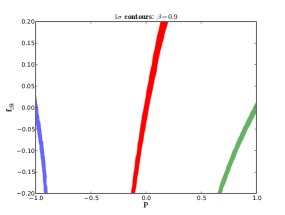
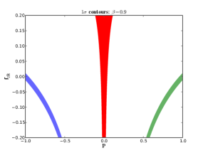
Suppose that an experimental measurement of corresponds to a true value of the parameters and . This measurement corresponds to an unknown point in the - plane. We define a region of siginificance around the point as the region where the value of the asymmetry is indistinguishable from the experimental value to within times the error in the measurement . In other words,
| (27) |
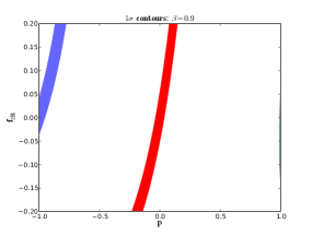
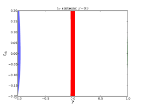
Since our purpose in this paper is to demonstrate the use of asymmetries, we choose a value for and ; evaluate using eq. 25 keeping only the statistical uncertainties and from the expressions of the corresponding distributions derived in the previous section. The results are shown in fig. 6.
IV.2 analysis
We combine three of the four asymmetries to make a statistic. One could combine all the four asymmetries to form a statistic. We have not considered such a combination in our analysis. This is because we consider, in our analysis, the case of highly boosted top quarks where effectively only two asymmetries and are sensitive to both and . Moreover, in the case of and , one can easily see from fig. 6 that the asymmetries and are similar in their abilty to constrain . Similarly, in the case of and , the bounds on are primarily due to and which can be seen from fig. 6. The asymmetries and are relatively poor in constraining . In both cases either one of and is sufficient to constrain (see fig. 6). Hence inclusion all the four asymmetries at a time in the analysis does not improve the best bounds obtained in the current analysis.
There are four ways in which three of the asymmetries can be combined. We discuss each of the combination. We assume that the asymmetries are measured independently and their errors are given according to either eq. 26 or eq. 25 depending on whether the systematic uncertainties are included or not. The is defined by
| (28) |
where .
Since our purpose is to demonstrate the utility of combining asymmetries, we calculate for a “true” value of and i.e and and evaluate for two cases. In the first case only statistical uncertainties are included in using eq. 25. In the second case the systematic uncertainties are also included in as given in eq. 26.
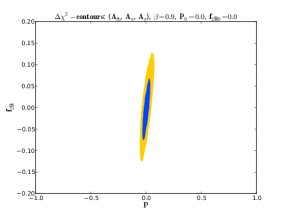
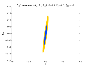
We give contours of values and corresponding to and confidence level (C.L) (for 2 degrees of freedom) respectively for both cases. As in the previous section we set and use the same number of events .
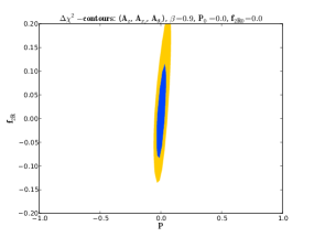

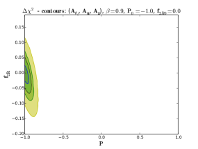
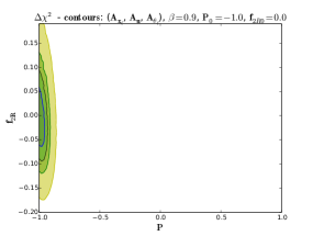
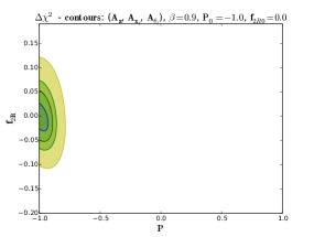
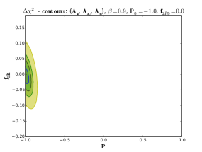
| combination | ||
|---|---|---|
Fig. 7 shows the contours for four different combinations of asymmetries for keeping only the statistical uncertainties. The effects of including systematic uncertainties of the asymmetries in the analysis are given later in the text. Table 1 gives the upper bound obtained on when , for different combinations of asymmetries, for . When the true value of and are the combination of , and and are better in constraining both and than the other two combinations.
IV.3 Limits on
| combination | ||
|---|---|---|
| (, , ) | ||
| (, , ) | ||
| (, , ) | ||
| (, , ) |
| combination | ||
|---|---|---|
| (, , ) | ||
| (, , ) | ||
| (, , ) | ||
| (, , ) |
In the table 2 and 3 we summarise the limits obtained on the anomalous coupling for two values of polarisation and keeping only statistical uncertainties. The best limits on obtained in our analysis assuming the top polarisation to be zero is . The sensitivity increases considerably if, for example, the expected polarization of the top would be . The corresponding limit on is: . Now we discuss the results after including systematic uncertainties of asymmetries using eq. 26 in eq. 28. The main effect of such inclusion is that the limits on and become weaker after the inclusion of systematic uncertainties. In particular, for the statistic does not constrain to between in the case of . In this case, one may need to use methods such as multivariate analysis, fit to the shape of the distributions, etc. to constrain and simultaneously. However, for large values of our observables are still sentitive to both and for values of upto as can be seen from fig. 8. A detailed analysis to estimate the systematic uncertainty on the asymmetries would take into account the effects of hadronisation, finite detector resolution etc on the measurement of asymmetries. Such an analysis would be very useful in improving the bounds on and compared to our simplified approach and is in progress.
Note that we have analyzed the case of pair production using events with invariant masses in the range to so as to analyse pairs possibly coming from a resonance. Even with an integrated luminosity of 100 fb-1 at TeV LHC, the number of top events in this analysis is considerably lower compared to the number used in the analyses such as Aguilar-Saavedra et al. (2007) which uses events over the entire range of the invariant mass. Due to the lower statistics our limits on for the case of zero polarisation are weaker compared to the limits obtained in Aguilar-Saavedra et al. (2007). But they are compatible with the CMS measurement of : using 2.2 of integrated luminosity at TeV. Note that our results are compatible with the result obtained by the CMS experiment with 2.2 fb-1 luminosity (corresponding to a number of events ) and hence smaller number of events than the ATLAS analysis, using the events with invariant-masses over the whole allowed range. This gives us confidence that the various limits indicated in this report are representative of what can be achieved in a real analysis. However, with this luminosity the observables are not sensitive to the contribution of the SM higher order corrections to the anomalous couplings, including . This is because their values are very small (see Sec. II) compared to the size of the bounds obtained in our analysis which are of the order of .
V Summary
In this work we have taken up the study of observables constructed out of kinematical variables of top decay products for the purpose of measuring top polarization in the presence of anomalous couplings as well as measuring the anomalous coupling itself. We concentrate on laboratory-frame variables which do not require the reconstruction of the top rest frame. An important consideration has been the degree of boost of the decaying top, since for many practical processes, as for example, a heavy resonance decaying into a top pair, the top quark is produced with large momentum in the lab frame.
We have considered four observables - asymmetries in the variables and . They are compared for their sensitivities to the polarisation of the top quark and the anomalous coupling . We state the results of the comparison of asymmetries in two categories: 1. Asymmetries for the measurement the top-quark polarisation , and 2. Asymmetries for the measurement of the anomalous coupling .
As for the first category of asymmetries for the measurement of the top-quark polarisation, for small values of boost from the top quark rest frame to the lab frame (), is the most sensitive observable. Next in sensitivity is as long as is small or negative. For large values of boosts (), and can be used as they are much more sensitive to compared to and .
For the second category corresponding to the measurement of the anomalous coupling , for all values of , can be used to measure as long as . For , , can be used to measure for any . The angular asymmetry is not suitable as a measure of for any value of as its sensitivity to is much more smaller than the sensitivities of and . Irrespective of the production mechanism of the top quark, can be used to measure at large values of the boost .
In all cases, we determine the and limits that the measurement of asymmetries can put on the determination of the polarisation or with a chosen number of events. We also do an analysis of the use of combination of asymmetries for the simultaneous determination of the top polarisation as well as . Finally we study the effects of including systematic uncertainties of asymmetries and find that for large values of top polarisation our observables are sensitive to both and for systematic uncertainties upto .
Note added: While our manuscript was in preparation a related work Cao et al. (2015) appeared. In this work, correlations of the anomalous couplings and are obtained through global fits to data on observables that are insensitive to the polarisation of the top. They point out the need of measuring the single top cross section to precision as this would put strong constraints on the new physics that affects the vertex. However, our method which uses observables sensitive to top polarisation, when used for processes such as single top production and decay, is sensitive to new physics even when the cross section is measured only to .
Appendix A The distribution
The differential distribution defined in the top quark rest frame is given by:
| (29) | ||||
where the cosine of the angle between the top spin direction and the lepton momentum and is as defined in eq. 10333We verified that upon integration over the azimuthal angles of the -quark and the lepton all the structures of eq. A8 of Bernreuther et al. (1992); *Erratum agree with those of our eq. 29. We have also checked that all the structures that appear in expression A8 of Bernreuther et al. (1992); *Erratum are present in intermediate stages of the calculations that lead to eq. 29.. It is also the polar angle of the lepton due to our choice of the top rest frame (see footnote in sec I). In the above equation, the top polarization points in the direction of motion of the top. When the top polarisation points in a general direction in the top rest frame the differential distribution of the top decay is given, to linear order in by:
| (30) | ||||
where and are the unit vectors along the direction of momenta of the lepton and the -quark in the top rest frame respectively; and are the azimuthal angles of the lepton and the -quark as mentioned in sec III.5.
Now we consider lab frame distributions. Let be the magnitude of the boost required to go from the top rest frame to the lab frame. The corresponding Lorentz transformation relates the energy and the polar angle of the lepton measured in these two frames by
| (31) | ||||
The inverse relations are
| (32) | ||||
Now the differential distribution is transformed to accordingly.
| (33) | ||||


Integrating the differential distribution over in the region bounded by eq. 32 gives the distribution .
The region of integration is given in fig. 9 for two different value of the boost chosen such that the left (right) figure corresponds to (). is the value of the boost where the lowest ordinate of the curve equals the maximum ordinate of the curve . As shown in fig. 9 the range of is divided into three regions, each having a separate integration limit on . For , we have where, , , , , For , the range of is divided into and for , . We first consider the case . The distribution is called in the region , in the region and in the region .
The expressions are given below for ():
| (34) | ||||
| (35) | ||||
| (36) | ||||
Similarly for , functions corresponding to the intervals ,, are called and respectively. We have and .
| (37) | ||||
Acknowledgements.
RMG wishes to acknowledge support from the Department of Science and Technology, India under Grant No. SR/S2/JCB-64/2007. SDR acknowledges support from the Department of Science and Technology, India, under the J.C. Bose National Fellowship programme, Grant No. SR/SB/JCB-42/2009.References
- Beringer et al. (2012) J. Beringer et al. (Particle Data Group), Phys.Rev. D86, 010001 (2012).
- Beneke et al. (2000) M. Beneke, I. Efthymiopoulos, M. L. Mangano, J. Womersley, A. Ahmadov, et al., (2000), arXiv:hep-ph/0003033 [hep-ph] .
- Han (2008) T. Han, Int.J.Mod.Phys. A23, 4107 (2008), arXiv:0804.3178 [hep-ph] .
- Bernreuther (2008) W. Bernreuther, J.Phys. G35, 083001 (2008), arXiv:0805.1333 [hep-ph] .
- Schilling (2012) F.-P. Schilling, Int.J.Mod.Phys. A27, 1230016 (2012), arXiv:1206.4484 [hep-ex] .
- Barberis (2013) E. Barberis, Int.J.Mod.Phys. A28, 1330027 (2013).
- Jabeen (2013) S. Jabeen, Int.J.Mod.Phys. A28, 1330038 (2013).
- Aad et al. (2013a) G. Aad et al. (ATLAS), Phys.Rev.Lett. 111, 232002 (2013a), arXiv:1307.6511 [hep-ex] .
- CMS (2012) CMS, W helicity in top pair events, Tech. Rep. CMS-PAS-TOP-11-020 (CERN, Geneva, 2012).
- Cheung (1996) K.-m. Cheung, Phys.Rev. D53, 3604 (1996), arXiv:hep-ph/9511260 [hep-ph] .
- Poulose and Rindani (1996) P. Poulose and S. D. Rindani, Phys. Rev. D 54, 4326 (1996).
- Poulose and Rindani (2000) P. Poulose and S. D. Rindani, Phys. Rev. D 61, 119901 (2000).
- Godbole et al. (2003) R. M. Godbole, S. D. Rindani, and R. K. Singh, Phys.Rev. D67, 095009 (2003), arXiv:hep-ph/0211136 [hep-ph] .
- Choudhury and Saha (2011) D. Choudhury and P. Saha, Pramana 77, 1079 (2011), arXiv:0911.5016 [hep-ph] .
- Gupta et al. (2009) S. K. Gupta, A. S. Mete, and G. Valencia, Phys.Rev. D80, 034013 (2009), arXiv:0905.1074 [hep-ph] .
- Hioki and Ohkuma (2011) Z. Hioki and K. Ohkuma, Phys.Rev. D83, 114045 (2011), arXiv:1104.1221 [hep-ph] .
- Choudhury and Saha (2012) D. Choudhury and P. Saha, JHEP 1208, 144 (2012), arXiv:1201.4130 [hep-ph] .
- Antipin and Valencia (2009) O. Antipin and G. Valencia, Phys.Rev. D79, 013013 (2009), arXiv:0807.1295 [hep-ph] .
- Bernreuther and Si (2013) W. Bernreuther and Z.-G. Si, Phys.Lett. B725, 115 (2013), arXiv:1305.2066 [hep-ph] .
- Buchmuller and Wyler (1986) W. Buchmuller and D. Wyler, Nucl.Phys. B268, 621 (1986).
- Grzadkowski et al. (2004) B. Grzadkowski, Z. Hioki, K. Ohkuma, and J. Wudka, Nucl.Phys. B689, 108 (2004), arXiv:hep-ph/0310159 [hep-ph] .
- Grzadkowski et al. (2010) B. Grzadkowski, M. Iskrzynski, M. Misiak, and J. Rosiek, JHEP 1010, 085 (2010), arXiv:1008.4884 [hep-ph] .
- Aguilar-Saavedra (2009) J. Aguilar-Saavedra, Nucl.Phys. B812, 181 (2009), arXiv:0811.3842 [hep-ph] .
- Bach and Ohl (2012) F. Bach and T. Ohl, Phys.Rev. D86, 114026 (2012), arXiv:1209.4564 [hep-ph] .
- Zhang and Willenbrock (2011) C. Zhang and S. Willenbrock, Phys.Rev. D83, 034006 (2011), arXiv:1008.3869 [hep-ph] .
- Fischer et al. (2002) M. Fischer, S. Groote, J. Korner, and M. Mauser, Phys.Rev. D65, 054036 (2002), arXiv:hep-ph/0101322 [hep-ph] .
- Czarnecki (1990) A. Czarnecki, Phys.Lett. B252, 467 (1990).
- Li et al. (1991) C. S. Li, R. J. Oakes, and T. C. Yuan, Phys.Rev. D43, 3759 (1991).
- Gonzalez-Sprinberg et al. (2011) G. A. Gonzalez-Sprinberg, R. Martinez, and J. Vidal, JHEP 1107, 094 (2011), arXiv:1105.5601 [hep-ph] .
- Jezabek and Kuhn (1989a) M. Jezabek and J. H. Kuhn, Nucl.Phys. B320, 20 (1989a).
- Czarnecki et al. (1991) A. Czarnecki, M. Jezabek, and J. H. Kuhn, Nucl.Phys. B351, 70 (1991).
- Kane et al. (1992a) G. L. Kane, G. A. Ladinsky, and C. P. Yuan, Phys. Rev. D 45, 124 (1992a).
- Bernreuther et al. (1992) W. Bernreuther, O. Nachtmann, P. Overmann, and T. Schröder, Nuclear Physics B 388, 53 (1992).
- (34) Erratum-ibid, Nuclear Physics B 406, 516 (1993).
- Jezabek and Kuhn (1994) M. Jezabek and J. H. Kuhn, Phys.Lett. B329, 317 (1994), arXiv:hep-ph/9403366 [hep-ph] .
- Nelson et al. (1997) C. A. Nelson, B. T. Kress, M. Lopes, and T. P. McCauley, Phys.Rev. D56, 5928 (1997), arXiv:hep-ph/9707211 [hep-ph] .
- Godbole et al. (2006) R. M. Godbole, S. D. Rindani, and R. K. Singh, JHEP 0612, 021 (2006), arXiv:hep-ph/0605100 [hep-ph] .
- Rindani (2000) S. D. Rindani, Pramana 54, 791 (2000), arXiv:hep-ph/0002006 [hep-ph] .
- Jezabek and Kuhn (1989b) M. Jezabek and J. H. Kuhn, Nucl.Phys. B314, 1 (1989b).
- Brandenburg et al. (2002) A. Brandenburg, Z. Si, and P. Uwer, Phys.Lett. B539, 235 (2002), arXiv:hep-ph/0205023 [hep-ph] .
- Bernreuther et al. (2004) W. Bernreuther, M. Fuecker, and Y. Umeda, Phys.Lett. B582, 32 (2004), arXiv:hep-ph/0308296 [hep-ph] .
- Groote et al. (2007) S. Groote, W. Huo, A. Kadeer, and J. Korner, Phys.Rev. D76, 014012 (2007), arXiv:hep-ph/0602026 [hep-ph] .
- Hagiwara et al. (2007) K. Hagiwara, K. Mawatari, and H. Yokoya, JHEP 0712, 041 (2007), arXiv:0707.3194 [hep-ph] .
- Kitadono and Li (2013) Y. Kitadono and H.-n. Li, Phys.Rev. D87, 054017 (2013), arXiv:1211.3260 [hep-ph] .
- Brucherseifer et al. (2013) M. Brucherseifer, F. Caola, and K. Melnikov, JHEP 1304, 059 (2013), arXiv:1301.7133 [hep-ph] .
- Bernreuther et al. (2014) W. Bernreuther, P. González, and C. Mellein, Eur.Phys.J. C74, 2815 (2014), arXiv:1401.5930 [hep-ph] .
- Bernreuther et al. (2006) W. Bernreuther, M. Fuecker, and Z.-G. Si, Phys.Rev. D74, 113005 (2006), arXiv:hep-ph/0610334 [hep-ph] .
- Bernreuther et al. (2008) W. Bernreuther, M. Fucker, and Z.-G. Si, Phys.Rev. D78, 017503 (2008), arXiv:0804.1237 [hep-ph] .
- Kuhn et al. (2007) J. H. Kuhn, A. Scharf, and P. Uwer, Eur.Phys.J. C51, 37 (2007), arXiv:hep-ph/0610335 [hep-ph] .
- Kühn et al. (2015) J. H. Kühn, A. Scharf, and P. Uwer, Phys. Rev. D 91, 014020 (2015).
- Mahlon and Parke (2000) G. Mahlon and S. J. Parke, Phys.Lett. B476, 323 (2000), arXiv:hep-ph/9912458 [hep-ph] .
- Schwienhorst et al. (2011) R. Schwienhorst, C.-P. Yuan, C. Mueller, and Q.-H. Cao, Phys.Rev. D83, 034019 (2011), arXiv:1012.5132 [hep-ph] .
- Dharmaratna and Goldstein (1990) W. G. Dharmaratna and G. R. Goldstein, Phys.Rev. D41, 1731 (1990).
- Kane et al. (1992b) G. L. Kane, G. A. Ladinsky, and C. P. Yuan, Phys. Rev. D 45, 124 (1992b).
- Bernreuther et al. (1996) W. Bernreuther, A. Brandenburg, and P. Uwer, Phys.Lett. B368, 153 (1996), arXiv:hep-ph/9510300 [hep-ph] .
- Baumgart and Tweedie (2013) M. Baumgart and B. Tweedie, JHEP 1308, 072 (2013), arXiv:1303.1200 [hep-ph] .
- Nojiri (1995) M. M. Nojiri, Phys.Rev. D51, 6281 (1995), arXiv:hep-ph/9412374 [hep-ph] .
- Perelstein and Weiler (2009) M. Perelstein and A. Weiler, JHEP 0903, 141 (2009), arXiv:0811.1024 [hep-ph] .
- Arai et al. (2010) M. Arai, K. Huitu, S. K. Rai, and K. Rao, JHEP 1008, 082 (2010), arXiv:1003.4708 [hep-ph] .
- Gopalakrishna et al. (2010) S. Gopalakrishna, T. Han, I. Lewis, Z.-g. Si, and Y.-F. Zhou, Phys.Rev. D82, 115020 (2010), arXiv:1008.3508 [hep-ph] .
- Godbole et al. (2010) R. M. Godbole, K. Rao, S. D. Rindani, and R. K. Singh, JHEP 1011, 144 (2010), arXiv:1010.1458 [hep-ph] .
- Huitu et al. (2011) K. Huitu, S. Kumar Rai, K. Rao, S. D. Rindani, and P. Sharma, JHEP 1104, 026 (2011), arXiv:1012.0527 [hep-ph] .
- Rindani and Sharma (2011) S. D. Rindani and P. Sharma, JHEP 1111, 082 (2011), arXiv:1107.2597 [hep-ph] .
- Biswal et al. (2013) S. S. Biswal, S. D. Rindani, and P. Sharma, Phys.Rev. D88, 074018 (2013), arXiv:1211.4075 [hep-ph] .
- Belanger et al. (2013a) G. Belanger, R. Godbole, L. Hartgring, and I. Niessen, JHEP 1305, 167 (2013a), arXiv:1212.3526 .
- Belanger et al. (2013b) G. Belanger, R. M. Godbole, S. Kraml, and S. Kulkarni, (2013b), arXiv:1304.2987 [hep-ph] .
- Taghavi and Najafabadi (2014) S. Taghavi and M. M. Najafabadi, Int.J.Theor.Phys. 53, 4326 (2014), arXiv:1301.3073 [hep-ph] .
- Aguilar-Saavedra and dos Santos (2014) J. Aguilar-Saavedra and S. A. dos Santos, Phys.Rev. D89, 114009 (2014), arXiv:1404.1585 [hep-ph] .
- Cao et al. (2011) J. Cao, L. Wu, and J. M. Yang, Phys.Rev. D83, 034024 (2011), arXiv:1011.5564 [hep-ph] .
- Choudhury et al. (2011) D. Choudhury, R. M. Godbole, S. D. Rindani, and P. Saha, Phys.Rev. D84, 014023 (2011), arXiv:1012.4750 [hep-ph] .
- Krohn et al. (2011) D. Krohn, T. Liu, J. Shelton, and L.-T. Wang, Phys.Rev. D84, 074034 (2011), arXiv:1105.3743 [hep-ph] .
- Falkowski et al. (2013) A. Falkowski, G. Perez, and M. Schmaltz, Phys.Rev. D87, 034041 (2013), arXiv:1110.3796 [hep-ph] .
- Godbole et al. (2012) R. M. Godbole, L. Hartgring, I. Niessen, and C. D. White, JHEP 1201, 011 (2012), arXiv:1111.0759 [hep-ph] .
- Randall and Sundrum (1999) L. Randall and R. Sundrum, Phys.Rev.Lett. 83, 3370 (1999), arXiv:hep-ph/9905221 [hep-ph] .
- Agashe et al. (2005) K. Agashe, R. Contino, and A. Pomarol, Nucl.Phys. B719, 165 (2005), arXiv:hep-ph/0412089 [hep-ph] .
- Agashe et al. (2008) K. Agashe, A. Belyaev, T. Krupovnickas, G. Perez, and J. Virzi, Phys.Rev. D77, 015003 (2008), arXiv:hep-ph/0612015 [hep-ph] .
- Shelton (2009) J. Shelton, Phys.Rev. D79, 014032 (2009), arXiv:0811.0569 [hep-ph] .
- Krohn et al. (2010) D. Krohn, J. Shelton, and L.-T. Wang, JHEP 1007, 041 (2010), arXiv:0909.3855 [hep-ph] .
- Bhattacherjee et al. (2013) B. Bhattacherjee, S. K. Mandal, and M. Nojiri, JHEP 1303, 105 (2013), arXiv:1211.7261 [hep-ph] .
- Kitadono and Li (2014) Y. Kitadono and H.-n. Li, Phys.Rev. D89, 114002 (2014), arXiv:1403.5512 [hep-ph] .
- Tweedie (2014) B. Tweedie, Phys.Rev. D90, 094010 (2014), arXiv:1401.3021 [hep-ph] .
- Chatrchyan et al. (2012) S. Chatrchyan et al. (CMS Collaboration), JHEP 1212, 015 (2012), arXiv:1209.4397 [hep-ex] .
- Chatrchyan et al. (2013) S. Chatrchyan et al. (CMS Collaboration), Phys.Lett. B720, 63 (2013), arXiv:1212.6175 [hep-ex] .
- Aad et al. (2012) G. Aad et al. (ATLAS Collaboration), Phys.Rev. D86, 091103 (2012), arXiv:1209.6593 [hep-ex] .
- Aad et al. (2013b) G. Aad et al. (ATLAS Collaboration), JHEP 1301, 116 (2013b), arXiv:1211.2202 [hep-ex] .
- Aad et al. (2013c) G. Aad et al. (ATLAS Collaboration), Phys.Rev. D88, 012004 (2013c), arXiv:1305.2756 [hep-ex] .
- Low (2013) I. Low, Phys.Rev. D88, 095018 (2013), arXiv:1304.0491 [hep-ph] .
- Hikasa et al. (1999) K.-i. Hikasa, J. M. Yang, and B.-L. Young, Phys.Rev. D60, 114041 (1999), arXiv:hep-ph/9908231 [hep-ph] .
- Nie et al. (2005) Y. M. Nie, C. S. Li, Q. Li, J. J. Liu, and J. Zhao, Phys.Rev. D71, 074018 (2005), arXiv:hep-ph/0501048 [hep-ph] .
- Jung et al. (2010) S. Jung, H. Murayama, A. Pierce, and J. D. Wells, Phys.Rev. D81, 015004 (2010), arXiv:0907.4112 [hep-ph] .
- Frampton et al. (2010) P. H. Frampton, J. Shu, and K. Wang, Phys.Lett. B683, 294 (2010), arXiv:0911.2955 [hep-ph] .
- Shu et al. (2010) J. Shu, T. M. P. Tait, and K. Wang, Phys. Rev. D 81, 034012 (2010).
- Cao et al. (2010) Q.-H. Cao, D. McKeen, J. L. Rosner, G. Shaughnessy, and C. E. M. Wagner, Phys. Rev. D 81, 114004 (2010).
- Dorsner et al. (2010) I. Dorsner, S. Fajfer, J. F. Kamenik, and N. Kosnik, Phys.Rev. D81, 055009 (2010), arXiv:0912.0972 [hep-ph] .
- Cheung et al. (2009) K. Cheung, W.-Y. Keung, and T.-C. Yuan, Phys.Lett. B682, 287 (2009), arXiv:0908.2589 [hep-ph] .
- Djouadi et al. (2010) A. Djouadi, G. Moreau, F. Richard, and R. K. Singh, Phys.Rev. D82, 071702 (2010), arXiv:0906.0604 [hep-ph] .
- Arhrib et al. (2010) A. Arhrib, R. Benbrik, and C.-H. Chen, Phys.Rev. D82, 034034 (2010), arXiv:0911.4875 [hep-ph] .
- Bai et al. (2011) Y. Bai, J. L. Hewett, J. Kaplan, and T. G. Rizzo, JHEP 1103, 003 (2011), arXiv:1101.5203 [hep-ph] .
- Gresham et al. (2011) M. I. Gresham, I.-W. Kim, and K. M. Zurek, Phys.Rev. D83, 114027 (2011), arXiv:1103.3501 [hep-ph] .
- Buckley et al. (2011) M. R. Buckley, D. Hooper, J. Kopp, and E. T. Neil, Phys. Rev. D 83, 115013 (2011).
- Bhattacherjee et al. (2011) B. Bhattacherjee, S. S. Biswal, and D. Ghosh, Phys.Rev. D83, 091501 (2011), arXiv:1102.0545 [hep-ph] .
- Aguilar-Saavedra and Perez-Victoria (2011a) J. Aguilar-Saavedra and M. Perez-Victoria, JHEP 1105, 034 (2011a), arXiv:1103.2765 [hep-ph] .
- Aguilar-Saavedra and Perez-Victoria (2011b) J. Aguilar-Saavedra and M. Perez-Victoria, JHEP 1109, 097 (2011b), arXiv:1107.0841 [hep-ph] .
- Chivukula et al. (2010) R. S. Chivukula, E. H. Simmons, and C.-P. Yuan, Phys.Rev. D82, 094009 (2010), arXiv:1007.0260 [hep-ph] .
- Grinstein et al. (2011) B. Grinstein, A. L. Kagan, M. Trott, and J. Zupan, Phys.Rev.Lett. 107, 012002 (2011), arXiv:1102.3374 [hep-ph] .
- Marques Tavares and Schmaltz (2011) G. Marques Tavares and M. Schmaltz, Phys.Rev. D84, 054008 (2011), arXiv:1107.0978 [hep-ph] .
- Jung et al. (2011) S. Jung, A. Pierce, and J. D. Wells, Phys.Rev. D83, 114039 (2011), arXiv:1103.4835 [hep-ph] .
- Ligeti et al. (2011) Z. Ligeti, G. Marques Tavares, and M. Schmaltz, JHEP 1106, 109 (2011), arXiv:1103.2757 [hep-ph] .
- Biswal et al. (2012) S. S. Biswal, S. Mitra, R. Santos, P. Sharma, R. K. Singh, et al., Phys.Rev. D86, 014016 (2012), arXiv:1201.3668 [hep-ph] .
- Allanach and Sridhar (2012) B. C. Allanach and K. Sridhar, Phys. Rev. D 86, 075016 (2012).
- Dupuis and Cline (2013) G. Dupuis and J. M. Cline, JHEP 1301, 058 (2013), arXiv:1206.1845 [hep-ph] .
- Aguilar-Saavedra (2014) J. Aguilar-Saavedra, Phys.Lett. B736, 132 (2014), arXiv:1405.1412 [hep-ph] .
- Cao et al. (2012) J. Cao, K. Hikasa, L. Wang, L. Wu, and J. M. Yang, Phys.Rev. D85, 014025 (2012), arXiv:1109.6543 [hep-ph] .
- Fajfer et al. (2012) S. Fajfer, J. F. Kamenik, and B. Melic, JHEP 1208, 114 (2012), arXiv:1205.0264 [hep-ph] .
- Grzadkowski and Hioki (2000) B. Grzadkowski and Z. Hioki, Phys.Lett. B476, 87 (2000), arXiv:hep-ph/9911505 [hep-ph] .
- Grzadkowski and Hioki (2002) B. Grzadkowski and Z. Hioki, Phys.Lett. B529, 82 (2002), arXiv:hep-ph/0112361 [hep-ph] .
- Grzadkowski and Hioki (2003) B. Grzadkowski and Z. Hioki, Phys.Lett. B557, 55 (2003), arXiv:hep-ph/0208079 [hep-ph] .
- Aguilar-Saavedra and Herrero-Hahn (2013) J. Aguilar-Saavedra and R. Herrero-Hahn, Phys.Lett. B718, 983 (2013), arXiv:1208.6006 [hep-ph] .
- Aguilar-Saavedra et al. (2007) J. Aguilar-Saavedra, J. Carvalho, N. F. Castro, F. Veloso, and A. Onofre, Eur.Phys.J. C50, 519 (2007), arXiv:hep-ph/0605190 [hep-ph] .
- Boos et al. (1999) E. Boos, L. Dudko, and T. Ohl, Eur.Phys.J. C11, 473 (1999), arXiv:hep-ph/9903215 [hep-ph] .
- Águila and Aguilar-Saavedra (2003) F. d. Águila and J. A. Aguilar-Saavedra, Phys. Rev. D 67, 014009 (2003).
- Hubaut et al. (2005) F. Hubaut, E. Monnier, P. Pralavorio, K. Smolek, and V. Simak, Eur.Phys.J. C44S2, 13 (2005), arXiv:hep-ex/0508061 [hep-ex] .
- Mohammadi Najafabadi (2007) M. Mohammadi Najafabadi, J.Phys. G34, 39 (2007), arXiv:hep-ph/0601155 [hep-ph] .
- Aguilar-Saavedra (2008) J. Aguilar-Saavedra, Nucl.Phys. B804, 160 (2008), arXiv:0803.3810 [hep-ph] .
- Najafabadi (2008) M. M. Najafabadi, JHEP 0803, 024 (2008), arXiv:0801.1939 [hep-ph] .
- Aguilar-Saavedra et al. (2008) J. Aguilar-Saavedra, J. Carvalho, N. F. Castro, A. Onofre, and F. Veloso, Eur.Phys.J. C53, 689 (2008), arXiv:0705.3041 [hep-ph] .
- Aguilar-Saavedra and Bernabeu (2010) J. Aguilar-Saavedra and J. Bernabeu, Nucl.Phys. B840, 349 (2010), arXiv:1005.5382 [hep-ph] .
- Rindani and Sharma (2012) S. D. Rindani and P. Sharma, Phys.Lett. B712, 413 (2012), arXiv:1108.4165 [hep-ph] .
- Boos et al. (2000) E. Boos, M. Dubinin, M. Sachwitz, and H. Schreiber, Eur.Phys.J. C16, 269 (2000), arXiv:hep-ph/0001048 [hep-ph] .
- Dutta et al. (2013) S. Dutta, A. Goyal, M. Kumar, and B. Mellado, (2013), arXiv:1307.1688 [hep-ph] .
- Lin et al. (2002) Z. Lin, T. Han, T. Huang, J. Wang, and X. Zhang, Phys.Rev. D65, 014008 (2002), arXiv:hep-ph/0106344 [hep-ph] .
- Devetak et al. (2011) E. Devetak, A. Nomerotski, and M. Peskin, Phys.Rev. D84, 034029 (2011), arXiv:1005.1756 [hep-ex] .
- Bernreuther et al. (2009) W. Bernreuther, P. Gonzalez, and M. Wiebusch, Eur.Phys.J. C60, 197 (2009), arXiv:0812.1643 [hep-ph] .
- Abazov et al. (2012) V. M. Abazov et al. (D0 Collaboration), Phys.Lett. B713, 165 (2012), arXiv:1204.2332 [hep-ex] .
- Grzadkowski and Misiak (2008) B. Grzadkowski and M. Misiak, Phys.Rev. D78, 077501 (2008), arXiv:0802.1413 [hep-ph] .
- Bernardo et al. (2014) C. Bernardo, N. F. Castro, M. C. N. Fiolhais, H. Gonçalves, A. G. C. Guerra, et al., Phys.Rev. D90, 113007 (2014), arXiv:1408.7063 [hep-ph] .
- Jezabek (1994) M. Jezabek, Nucl.Phys.Proc.Suppl. 37B, 197 (1994), arXiv:hep-ph/9406411 [hep-ph] .
- ATL (2010) Prospects for top anti-top resonance searches using early ATLAS data., Tech. Rep. ATL-PHYS-PUB-2010-008 (CERN, Geneva, 2010).
- Berger et al. (2012) E. L. Berger, Q.-H. Cao, J.-H. Yu, and H. Zhang, Phys.Rev.Lett. 109, 152004 (2012), arXiv:1207.1101 [hep-ph] .
- Papaefstathiou and Sakurai (2012) A. Papaefstathiou and K. Sakurai, JHEP 1206, 069 (2012), arXiv:1112.3956 [hep-ph] .
- Ahrens et al. (2010) V. Ahrens, A. Ferroglia, M. Neubert, B. D. Pecjak, and L. L. Yang, JHEP 1009, 097 (2010), arXiv:1003.5827 [hep-ph] .
- Cao et al. (2015) Q.-H. Cao, B. Yan, J.-H. Yu, and C. Zhang, (2015), arXiv:1504.03785 [hep-ph] .