Time-Inconsistent Planning: A Computational Problem in Behavioral Economics

In many settings, people exhibit behavior that is inconsistent across time — we allocate a block of time to get work done and then procrastinate, or put effort into a project and then later fail to complete it. An active line of research in behavioral economics and related fields has developed and analyzed models for this type of time-inconsistent behavior.

Here we propose a graph-theoretic model of tasks and goals, in which dependencies among actions are represented by a directed graph, and a time-inconsistent agent constructs a path through this graph. We first show how instances of this path-finding problem on different input graphs can reconstruct a wide range of qualitative phenomena observed in the literature on time-inconsistency, including procrastination, abandonment of long-range tasks, and the benefits of reduced sets of choices. We then explore a set of analyses that quantify over the set of all graphs; among other results, we find that in any graph, there can be only polynomially many distinct forms of time-inconsistent behavior; and any graph in which a time-inconsistent agent incurs significantly more cost than an optimal agent must contain a large “procrastination” structure as a minor. Finally, we use this graph-theoretic model to explore ways in which tasks can be designed to help motivate agents to reach designated goals.

1 Introduction

A fundamental issue in behavioral economics — and in the modeling of individual decision-making more generally — is to understand the effects of decisions that are inconsistent over time. Examples of such inconsistency are widespread in everyday life: we make plans for completing a task but then procrastinate; we put work into getting a project partially done but then abandon it; we pay for gym memberships but then fail to make use of them. In addition to analyzing and modeling these effects, there has been increasing interest in incorporating them into the design of policies and incentive systems in domains that range from health to personal finance.

These types of situations have a recurring structure: a person makes a plan at a given point in time for something they will do in the future (finishing homework, exercising, paying off a loan), but at a later point in time they fail to follow through on the plan. Sometimes this failure is the result of unforeseen circumstances that render the plan invalid — a person might join a gym but then break their leg and be unable to exercise — but in many cases the plan is abandoned even though the circumstances are essentially the same as they were at the moment the plan was made. This presents a challenge to any model of planning based on optimizing a utility function that is consistent over time: in an optimization framework, the plan must have been an optimal choice at the outset, but later it was optimal to abandon it. A line of work in the economics literature has thus investigated the properties of planning with objective functions that vary over time in certain natural and structured ways.

A Basic Example and Model. To introduce these models, it is useful to briefly describe an example due to George Akerlof [1], with the technical details adapted slightly for the discussion here. (The story will be familiar to readers who know Akerlof’s paper; we cover it in some detail because it will motivate a useful and recurring construction later in the work.) Imagine a decision-making agent — Akerlof himself, in his story — who needs to ship a package sometime during one of the next $n$ days, labeled $t=1,2,\ldots,n$, and must decide on which day $t$ to do so. Each day that the package has not reached its destination results in a cost of $x$ (per day), due to the lack of use of the package’s contents. If we suppose that the package takes a constant $h$ days in transit, this means a cost of $(t+h)x$ if it is shipped on day $t$. Also, shipping the package is an elaborate operation that will result in one-time cost of $c$, due to the amount of time involved in getting it sent out. The package must be shipped during one of the $n$ specified days.

What is the optimal plan for shipping the package? Clearly the cost $c$ will be incurred exactly once regardless of the day on which it is shipped, and there will also be a cost of $(t+h)x$ if it is shipped on day $t$. Thus we are minimizing $c+tx+hx$ subject to $1\leq t\leq n$; since everything but $t$ is a constant in the objective function, the cost is clearly minimized by setting $t=1$. In other words, the agent should ship the package right away.

But in Akerlof’s story, he did something that should be familiar from one’s own everyday experience: he procrastinated. Although there were no unexpected changes to the trade-offs involved in shipping the package, when each new day arrived there seemed to be other things that were more crucial than sending it out that day, and so each day he resolved that he would instead send it tomorrow. The result was that the package was not sent out until the end of the time period. (In fact, he sent it a few months into the time period once something unexpected did happen to change the cost structure — a friend offered to send it for him as part of a larger shipment — though this wrinkle is not crucial for the story.)

There is a natural way to model an agent’s decision to procrastinate, using the notion of present bias — the tendency to view costs and benefits that are incurred at the present moment to be more salient than those incurred in the future. In particular, suppose that for a constant $b>1$, costs that one must incur in the current time period are increased by a factor of $b$ in one’s evaluation. Then in Akerlof’s example, when the agent on day $t$ is considering the decision to send the package, the cost of sending it on day $t$ is $bc+(t+h)x$, while the cost of sending it on day $(t+1)$ is $c+(t+1+h)x$. The difference between these two costs is $(b-1)c-x$, and so if $(b-1)c>x$, the agent will decide on each day $t$ that the optimal plan is to wait until day $t+1$; things will continue this way until day $n$, when waiting is no longer an option and the package must be sent.

Quasi-Hyperbolic Discounting. Building on considerations such as those above, and others in earlier work in economics [14, 12], a significant amount of work has developed around a model of time-inconsistency known as quasi-hyperbolic discounting [8]. In this model, parametrized by quantities $\beta,\delta\leq 1$, a cost or reward of value $c$ that will be realized at a point $t\geq 1$ time units into the future is evaluated as having a present value of $\beta\delta^{t}c$. (In other words, values at time $t$ are discounted by a factor of $\beta\delta^{t}$.) With $\beta=1$ this is the standard functional form for exponential discounting, but when $\beta<1$ the function captures present bias as well: values in the present time period are scaled up by $\beta^{-1}$ relative to all other periods. (In what follows, we will consistently use $b$ to denote $\beta^{-1}$.)

Research on this $(\beta,\delta)$-model of discounting has been extensive, and has proceeded in a wide variety of directions; see Frederick et al. [6] for a review. To keep our analysis clearly delineated in scope, we make certain decisions at the outset relative to the full range of possible research questions: we focus on a model of agents who are naive, in that they do not take their own time-inconsistency into account when planning; we do not attempt to derive the $(\beta,\delta)$-model from more primitive assumptions but rather take it as a self-contained description of the agent’s observed behavior; and we discuss the case of $\delta=1$ so as to focus attention on the present-bias parameter $\beta$. Note that the initial Akerlof example has all these properties; it is essentially described in terms of the $(\beta,\delta)$-model with an agent who is naive about his own time-inconsistency, with $\delta=1$, and with $\beta=b^{-1}$ (using the parameter $b$ from that discussion).

Our starting point in this paper is to think about some of the qualitative predictions of the $(\beta,\delta)$-model, and how to analyze them in a unified framework. In particular, research in behavioral economics has shown how agents making plans in this model can exhibit the following behaviors.

1. Procrastination, as discussed above.

2. Abandonment of long-range tasks, in which a person starts on a multi-stage project but abandons it in the middle, even though the underlying costs and benefits of the project have remained essentially unchanged [11].

3. The benefits of choice reduction, in which reducing the set of options available to an agent can actually help them reach a goal more efficiently [10, 7]. A canonical example is the way in which imposing a deadline can help people complete a task that might not get finished in the absence of a deadline [2].

These consequences of time-inconsistency, as well as a number of others, have in general each required their own separate and sometimes quite intricate modeling efforts. It is natural to ask whether there might instead be a single framework for representing tasks and goals in which all of these effects could instead emerge “mechanically,” each just as a different instance of the same generic computational problem. With such a framework, it would become possible to search for worst-case guarantees, by quantifying over all instances, and to talk about designing or modifying given task structures to induce certain desired behaviors.

The present work: A graph-theoretic model. Here we propose such a framework, using a graph-theoretic formulation. We consider an agent with present-bias parameter $\beta$ who must construct a path in a directed acyclic graph $G$ with edge costs, from a designated start node $s$ to a designated target node $t$. We will call such a structure a task graph. Informally, the nodes of the task graph represent states of intermediate progress toward the goal $t$, and the edges represent transitions between them. Directed graphs have been shown to have considerable expressive power for planning problems in the artificial intelligence literature [13]; this provides evidence for the robustness of a graph-based approach in representing these types of decision environments. Our concerns in this work, however, are quite distinct from the set of graph-based planning problems in artificial intelligence, since our aim is to study the particular consequences of time-inconsistency in these domains.

A sample instance of this problem is depicted in Figure 1, with the costs drawn on the edges. When the agent is standing at a node $v$, it determines the minimum cost of a path from $v$ to $t$, but it does so using its present-biased evaluation of costs: the cost of the first edge on the path (starting from $v$) is evaluated according to the true cost, and all subsequent edges have their costs reduced by $\beta$. If the agent chooses path $P$, it follows just the first edge $(v,w)$ of $P$, and then it re-evaluates which path to follow using this same present-biased evaluation but now from the node $w$. In this way, the agent iteratively constructs a path from $s$ to $t$.

In the next section we will show how our graph-theoretic model easily captures time-inconsistency phenomena including procrastination, abandonment, and choice reduction. But to make the definitions concrete, it is useful to work through the agent’s computation on the graph depicted in Figure 1. In Figure 1, an agent that has a present-bias parameter of $\beta=1/2$ needs to go from $s$ to $t$. From $s$, the agent evaluates the path $s$-$a$-$b$-$t$ as having cost $16+2\beta+2\beta=18$, the path $s$-$c$-$d$-$t$ as having cost $8+8\beta+8\beta=16$, and the path $s$-$c$-$e$-$t$ as having cost $8+2\beta+16\beta=17$. Thus the agent traverses the edge $(s,c)$ and ends up at $c$. From $c$, the agent now evaluates the path $c$-$d$-$t$ as having cost $8+8\beta=12$ and the path $c$-$e$-$t$ as having cost $2+16\beta=10$, and so the agent traverses the edge $(c,e)$ and then (having no further choices) continues on the edge $(e,t)$.

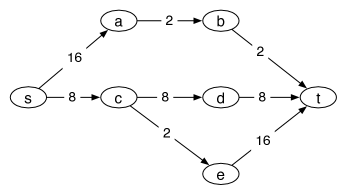
Figure 1: A present-biased agent must choose a path from $s$ to $t$.

This example illustrates a few points. First, when the agent set out on the edge $(s,c)$, it was intending to next follow the edge $(c,d)$, but when it got to $c$, it changed its mind and followed the edge $(c,e)$. A time-consistent agent (with $\beta=1$), by contrast, would never do this; the path it decides to take starting at $s$ is the path it will continue to follow all the way to $t$. Second, we are interested in whether the agent minimizes the cost of traveling from $s$ to $t$ according to the real costs, not according to its evaluation of the costs, and in this regard it fails to do so; the shortest path is $s$-$a$-$b$-$t$, with a cost of $20$, while the agent incurs a cost of $26$.

Overview of Results. Our graph-theoretic framework makes it possible to reason about time-inconsistency effects that arise in very different settings, provided simply that the underlying decisions faced by the agent can be modeled as the search for a path through a graph-structured sequence of options. And perhaps more importantly, since it is tractable to ask questions that quantify over all possible graphs, we can cleanly compare different scenarios, and search for the best or worst possible structures relative to specific objectives. This is difficult to do without an underlying combinatorial structure. For example, suppose we were inspired by Akerlof’s example to try identifying the scenario in which time-inconsistency leads to the greatest waste of effort. A priori, it is not clear how to formalize the search over all possible “scenarios.” But as we will see, this is precisely something we can do if we simply ask for the graph in which time-inconsistency produces the greatest ratio between the cost of the path traversed and cost of the optimal path.

Moreover, with this framework in place, it becomes easier to express formal questions about design for these contexts: if as a designer of a complex task we are able to specify the underlying graph structure, which graphs will lead time-inconsistent agents to reach the goal as efficiently as possible?

Our core questions are based on quantifying the inefficiency from time-inconsistent behavior, designing task structures to reduce this inefficiency, and comparing the behavior of agents with different levels of time-inconsistency. Specifically, we ask:

1. In which graph structures does time-inconsistent planning have the potential to cause the greatest waste of effort relative to optimal planning?

2. How do agents with different levels of present bias (encoded as different values of $\beta$) follow combinatorially different paths through a graph toward the same goal?

3. Can we increase an agent’s efficiency in reaching a goal by deleting nodes and/or edges from the underlying graph, thus reducing the number of options available?

4. How do we structure tasks for a heterogeneous collection of agents with diverse values of $\beta$, so that each agent either reaches the goal or abandons it quickly without wasting effort?

In what follows, we address these questions in turn. For the first question, we consider $n$-node graphs and ask how large the cost ratio can be between the path followed by a present-biased agent and the path of minimum total cost. Since deviations from the minimum-cost plan due to present bias are sometimes viewed as a form of “irrational” behavior, this cost ratio effectively serves as a “price of irrationality” for our system. We give a characterization of the worst-case graphs in terms of graph minors; this enables us to show, roughly speaking, that any instance with sufficiently high cost ratio must contain a large instance of the Akerlof example embedded inside it.

For the second question, we consider the possible paths followed by agents with different present-bias parameters $\beta$. As we sweep $\beta$ over the interval $[0,1]$, we have a type of parametric path problem, where the choice of path is governed by a continuous parameter ($\beta$ in this case). We show that in any instance, the number of distinct paths is bounded by a polynomial function of $n$, which forms an interesting contrast with canonical formulations of the parametric shortest-path problem, in which the number of distinct paths can be superpolynomial in $n$ [3, 9].

The third and fourth questions are essentially design questions: we must design a set of tasks to optimize the performance of a present-biased agent. For the third question, we show how it is possible for agents to be more efficient when nodes and/or edges are deleted from the underlying graph; on the other hand, if we want to motivate an agent to follow a particular path $P$ through the graph, it can be crucial to present the agent with a subgraph that includes not just $P$ but also certain additional nodes and edges that do not belong to $P$. We give a graph-theoretic characterization of the possible subgraphs supporting efficient traversal. Finally, for heterogeneous agents, we explore a simple variant of the problem based on partitioning large tasks into smaller ones.

Before turning to these questions, we first discuss the basic graph-theoretic problem in more detail, showing how instances of this problem capture the time-inconsistency phenomena discussed earlier in this section.

2 The Graph-Theoretic Model

In order to argue that our graph-theoretic model captures a variety of phenomena that have been studied in connection with time-inconsistency, we present a sequence of examples to illustrate some of the different behaviors that the model exhibits. We note that the example in Figure 1 already illustrates two simple points: that the path chosen by the agent can be sub-optimal; and that even if the agent traverses an edge $e$ with the intention of following a path $P$ that begins with $e$, it may end up following a different path $P^{\prime}$ that also begins with $e$.

For an edge $e$ in $G$, let $c(e)$ denote the cost of $e$; and for a path $P$ in $G$, let $e_{i}(P)$ denote the $i^{\rm th}$ edge on $P$. In terms of this notation, the agent’s decision is easy to specify: when standing at a node $v$, it chooses the path $P$ that minimizes $c(e_{1}(P))+\beta\sum_{i>1}c(e_{i}(P))$ over all $P$ that run from $v$ to $t$. It follows the first edge of $P$ to a new node $w$, and then performs this computation again.

We begin by observing that Figure 2(a) represents a version of the Akerlof example from the introduction. (For simplicity we assume that the delivery of the package is instantaneous, so $h=0$. Also recall that we use $b$ to denote $\beta^{-1}$.) Node $t$ represents the state in which the agent has sent the package, and node $v_{i}$ represents the state in which the agent has reached day $i$ without sending the package. The agent has the option of going directly from node $s$ to node $t$, and this is the shortest $s$-$t$ path. But if $(b-1)c>bx$, then the agent will instead go from $s$ to $v_{1}$, intending to complete the path $s$-$v_{1}$-$t$ in the next time step. At $v_{1}$, however, the agent decides to go to $v_{2}$, intending to complete the path $v_{1}$-$v_{2}$-$t$ in the next time step. This process continues: the agent, following exactly the reasoning in the example from the introduction, is procrastinating and not going to $t$, and in the end its path goes all the way to the last node $v_{n}$ ($n=5$ in the figure) before finally taking an edge to $t$. (One minor change from the set-up in the introduction is the fact that the present-bias effect here holds more consistently, and is applied to $x$ as well; this has no real effect on the underlying story.)

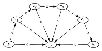
(a) The Akerlof example

(b) Homework deadlines

Figure 2: Path problems that exhibit procrastination, abandonment, and choice reduction.

Extending the model to include rewards. Thus far we can’t talk about an agent who abandons its pursuit of the goal midway through, since our model requires the agent to construct a path that goes all the way to $t$. But a simple extension of the model makes it possible to consider such situations.

Suppose we place a reward of $r$ at the target node $t$, which will be claimed if the agent reaches $t$. Standing at a node $v$, the agent now has an expanded set of options: it can follow an edge out of $v$ as before, or it can quit taking steps, incurring no further cost but also not claiming the reward. The agent will choose the latter option precisely when either there is no $v$-$t$ path, or when the minimum cost of a $v$-$t$ path exceeds the value of the reward, evaluated in light of present bias: $c(e_{1}(P))+\beta\sum_{i>1}c(e_{i}(P))>\beta r$ for all $v$-$t$ paths $P$. It is important to note a key feature of this evaluation: the reward is always discounted by $\beta$ relative to the cost that is being incurred in the current period, even if the reward will be received right after this cost is incurred. (For example, if the path $P$ has a single edge, then the agent is comparing $c(e_{1}(P))$ to $\beta r$.)

In what follows, we will consider both these models: the former fixed-goal model, in which the agent must reach $t$ and seeks to minimize its cost; and the latter reward model in which the agent trades off cost incurred against reward at $t$, and has the option of stopping partway to $t$. Aside from this distinction, both models share the remaining ingredients, based on traversing an $s$-$t$ path in $G$.

It is easy to see that the reward model displays the phenomenon of abandonment, in which the agent spends some cost to try reaching $t$, but then subsequently gives up without receiving the reward. Consider for example a three-node path on nodes $s$, $v_{1}$, and $t$, with an edge $(s,v_{1})$ of cost $1$ and an edge $(v_{1},t)$ of cost $4$. If $\beta=1/2$ and there is a reward of $7$ at $t$, then the agent will traverse the edge $(s,v_{1})$ because it evaluates the total cost of the path at $1+4\beta=3<7\beta=3.5$. But once it reaches $v_{1}$, it evaluates the cost of completing the path at $4>7\beta=3.5$, and so it quits without reaching $t$.

An example involving choice reduction. It is useful to describe a more complex example that shows the modeling power of this shortest-path formalism, and also shows how we can use the model to analyze deadlines as a form of beneficial choice reduction. (As should be clear, with a time-consistent agent it can never help to reduce the set of choices; such a phenomenon requires some form of time-inconsistency.) First we describe the example in text, and then show how to represent it as a graph.

Imagine a student taking a three-week short course in which the required work is to complete two small projects by the end of the course. It is up to the student when to do the projects, as long as they are done by the end. The student incurs an effort cost of $1$ from any week in which she does no projects (since even without projects there is still the lower-level effort of attending class), a cost of $4$ from any week in which she does one project, and a cost of $9$ from any week in which she does both projects. Finally, the student receives a reward of $16$ for completing the course, and she has a present-bias parameter of $\beta=1/2$.

Figure 2(b) shows how to represent this scenario using a graph. Node $v_{ij}$ corresponds to a state in which $i$ weeks of the course are finished, and the student has completed $j$ projects so far; we have $s=v_{00}$ and $t=v_{32}$. All edges go one column to the right, indicating that one week will elapse regardless; what is under the student’s control is how many rows the edge will span. Horizontal edges have cost $1$, edges that descend one row have cost $4$, and edges that descend two rows in a single hop have cost $9$. In this way, the graph precisely represents the story just described.

How does the student’s construction of an $s$-$t$ path work out? From $s$, she goes to $v_{10}$ and then to $v_{20}$, intending to complete the path to $t$ via the edge $(v_{20},t)$. But at $v_{20}$, she evaluates the cost of the edge $(v_{20},t)$ as $9>\beta r=16/2=8$, and so she quits without reaching $t$. The story is thus a familiar one: the student plans to do both projects in the final week of the course, but when she reaches the final week, she concludes that it would be too costly and so she drops the course instead.

The instructor can prevent this from happening through a very simple intervention. If he requires that the first project be completed by the end of the second week of the course, this corresponds simply to deleting node $v_{20}$ from the graph. With $v_{20}$ gone, the path-finding problem changes: now the student starting at $s$ decides to follow the path $s$-$v_{10}$-$v_{21}$-$t$, and at $v_{10}$ and then $v_{21}$ she continues to select this path, thereby reaching $t$. Thus, by reducing the set of options available to the student — and in particular, by imposing an intermediate deadline to enforce progress — the instructor is able to induce the student to complete the course.

There are many stories like this one about homework and deadlines, and our point is not to focus too closely on it in particular. Indeed, to return to one of the underpinnings of our graph-theoretic formalism, our point is in a sense the opposite: it is hard to reason about the space of possible “stories,” whereas it is much more tractable to think about the space of possible graphs. Thus by encoding the set of stories mechanically in the form of graphs, it becomes feasible to reason about them as a whole.

We have thus seen how a number of different time-inconsistency phenomena arise in simple instances of the path-finding problem. The full power of the model, however, lies in proving statements that quantify over all graphs; we begin this next.

3 The Cost Ratio: A Characterization Via Graph Minors

Our path-finding model naturally motivates a basic quantity of interest: the cost ratio, defined as the ratio between the cost of the path found by the agent and the cost of the shortest path. We work here within the fixed-goal version of the model, in which the agent is required to reach the goal $t$ and the objective is to minimize the cost of the path used.

To fix notation for this discussion, given a directed acyclic graph $G$ on $n$ nodes with positive edge costs, we let $d(v,w)$ denote the cost of the shortest $v$-$w$ path in $G$, when one exists (using the true edge costs, not modified by present bias). We are given designated start and end nodes $s$ and $t$ respectively, and we pre-process the graph by deleting every node that is either not reachable from $s$ or that cannot reach $t$. Let ${P_{\beta}}(v,t)$ denote the the $v$-$t$ path followed by an agent with present-bias $\beta$, and let ${c_{\beta}}(v,t)$ be the total cost of this path. The cost ratio can thus be written as ${c_{\beta}}(s,t)/d(s,t)$.

A bad example for the cost ratio. We first describe a simple construction showing that the cost ratio can be exponential in the number of nodes $n$. We then move on to the main result of this section, which is a characterization of the instances in which the cost ratio achieves this exponential lower bound.

Our construction is an adaptation of the Akerlof example from the introduction. We describe it using edges of zero cost, but it is easy to modify it to give all edges positive cost. We have a graph that consists of a directed path $s=v_{0},v_{1},v_{2},\ldots,v_{n}$, and with each $v_{i}$ also linking directly to node $t$. (The case $n=5$ is the graph in Figure 2(a).) With $b=\beta^{-1}$, we choose any $\mu<b$; we let the cost of the edge $(v_{j},t)$ be $\mu^{j}$, and let the cost of each edge $(v_{j},v_{j+1})$ be $0$.

Now, when the agent is standing at node $v_{j}$, it evaluates the cost of going directly to $t$ as $\mu^{j}$, while the cost of the two-step path through $v_{j+1}$ to $t$ is evaluated as $0+\beta\mu^{j+1}=(\beta\mu)\mu^{j}<\mu^{j}$. Thus the agent will follow the edge $(v_{j},v_{j+1})$ with the plan of continuing from $v_{j+1}$ to $t$. But this holds for all $j$, so once it reaches $v_{j+1}$, it changes its mind and continues on to $v_{j+2}$, and so forth. Ultimately it reaches $v_{n}$, and then must go directly to $t$ at a cost of ${c_{\beta}}(s,t)=\mu^{n}$. Since $d(s,t)=1$ by using the edge directly from $s$ to $t$, this establishes the exponential lower bound on the cost ratio ${c_{\beta}}(s,t)/d(s,t)$. Essentially, this construction shows that the Akerlof example can be made quantitatively much worse than its original formulation by having the cost of going directly to the goal grow by a modest constant factor in each time step; when a present-biased agent procrastinates in this case, it ultimately incurs an exponentially large cost.

As noted above, the fact that some edges in this example have zero cost is not crucial; we could give each edge $(v_{j},v_{j+1})$ a uniform cost ${\varepsilon}>0$ and correspondingly reduce the value of $\mu$ slightly.

A Graph Minor Characterization. We now provide a structural description of the graphs on which the cost ratio can be exponential in the number of nodes $n$ — essentially we show that a constant fraction of the nodes in such a graph must have the structure of the Akerlof example.

We make this precise using the notion of a minor. Given two undirected graphs $H$ and $K$, we say that $H$ contains a $K$-minor if we can map each node $\kappa$ of $K$ to a connected subgraph $S_{\kappa}$ in $H$, with the properties that (i) $S_{\kappa}$ and $S_{\kappa^{\prime}}$ are disjoint for every two nodes $\kappa,\kappa^{\prime}$ of $K$, and (ii) if $(\kappa,\kappa^{\prime})$ is an edge of $K$, then in $H$ there is some edge connecting a node in $S_{\kappa}$ to a node in $S_{\kappa^{\prime}}$. Informally, the definition means that we can build a copy of $K$ using the structure of $H$, with disjoint connected subgraphs of $H$ playing the role of “super-nodes” that represent the nodes of $K$, and with the adjacencies among these super-nodes representing the adjacencies in $K$. The minor relation shows up in many well-known results in graph theory, perhaps most notably in Kuratowski’s Theorem that a non-planar graph must contain either the complete graph $K_{5}$ or the complete bipartite graph $K_{3,3}$ as a minor [4].

Our goal here is to show that if $G$ has exponential cost ratio, then its undirected version must contain a large copy of the graph underlying the Akerlof example as a minor. In other words, the Akerlof example is not only a way to produce a large cost ratio, but it is in a sense an unavoidable signature of any example in which the cost ratio is very large.

We set this up as follows. Let ${\sigma}(G)$ denote the skeleton of $G$, the undirected graph obtained by removing the directions on the edges of $G$. Let ${\cal F}_{k}$ denote the graph with nodes $v_{1},v_{2},\ldots,v_{k}$, and $w$, and edges $(v_{i},v_{i+1})$ for $i=1,\ldots,k-1$, and $(v_{i},w)$ for $i=1,\ldots,k$. We refer to ${\cal F}_{k}$ as the $k$-fan.

We now claim

Theorem 3.1

For every $\lambda>1$ there exist $n_{0}>0$ and ${\varepsilon}>0$ such that if $n\geq n_{0}$ and ${c_{\beta}}(s,t)/d(s,t)>\lambda^{n}$, then ${\sigma}(G)$ contains an ${\cal F}_{k}$-minor for some $k\geq{\varepsilon}n$.

Proof:   The idea behind the proof is as follows. For each node, we consider a “rounded” version of its distance to $t$ — essentially the logarithm of its distance to $t$, truncated down to an integer value. We argue that there exists a node $v$ on the path taken by the agent for which this quantity is large, and we consider the portion $P$ of this path that runs from $s$ to $v$. From many nodes on $P$, other paths emanate back to $t$ that remain disjoint from $P$. These other paths together with $P$ provide us with the structure from which we can build an ${\cal F}_{k}$-minor.

We now give the detailed argument. For each node $v$, we define the rank of $v$, denoted $r(v)$, to be $0$ if $d(v,t)\leq d(s,t)$, and otherwise it is the minimum integer $j>0$ such that $d(v,t)\leq b^{j}d(s,t)$.

Here is a first basic fact about ranks.

(A) If $(v,w)$ is an edge on ${P_{\beta}}(s,t)$, then $r(w)\leq r(v)+1$.

To prove (A), consider an edge $(v,w)$ on ${P_{\beta}}(s,t)$. If $(v,w)$ lies on a shortest path from $v$ to $t$, then $d(w,t)\leq d(v,t)$ and hence $r(w)\leq r(v)$. Otherwise, let $(v,w^{\prime})$ be an edge on a shortest $v$-$t$ path; the agent’s decision to traverse the edge $(v,w)$ means that

$$c(v,w)+\beta d(w,t)\leq c(v,w^{\prime})+\beta d(w^{\prime},t)\leq d(v,t),$$

and hence $d(w,t)\leq bd(v,t)$. It follows that $r(w)\leq r(v)+1$.

Now, suppose that ${c_{\beta}}(s,t)>\lambda^{n}d(s,t)$. For future use, we choose constants $n_{0}>0$ and $\lambda_{0}>1$ such that when $n\geq n_{0}$, we have $n\lambda_{0}^{n}<\lambda^{n}$. We then set ${\varepsilon}=\log_{b}\lambda_{0}$.

We now claim

(B) There exists an edge $(v,w)$ on ${P_{\beta}}(s,t)$ of cost $>\lambda_{0}^{n}d(s,t)$.

To prove (B), we observe that since the quantity ${c_{\beta}}(s,t)$ is a sum of at most $n$ terms, corresponding to the edge costs in ${P_{\beta}}(s,t)$, there exists at least one term in this sum that is $>\lambda^{n}d(s,t)/n$. Suppose it is the cost of the edge $(v,w)$ on ${P_{\beta}}(s,t)$; i.e. $c(v,w)>\lambda^{n}d(s,t)/n$. By our choice of $n_{0}$ and $\lambda_{0}$, we then have $c(v,w)>\lambda_{0}^{n}d(s,t)$ when $n\geq n_{0}$.

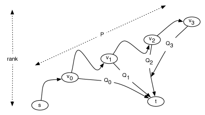
Figure 3: The construction of an ${\cal F}_{k}$-minor in Theorem 3.1.

Next we claim

(C) There exists a node $v$ on ${P_{\beta}}(s,t)$ of rank at least ${\varepsilon}n$.

Indeed, the tail $v$ of the edge $(v,w)$ from (B) has rank at least ${\varepsilon}n$. To see this, consider the agent’s decision at node $v$, when it chooses to pay $c(v,w)>\lambda_{0}^{n}d(s,t)$ on its next step. If $(v,w^{\prime})$ is the first edge on a shortest $v$-$t$ path, then we have $d(v,t)=c(v,w^{\prime})+d(w^{\prime},t)\geq c(v,w^{\prime})+\beta d(w^{\prime},t)\geq c(v,w)+\beta d(w,t)\geq c(v,w)>\lambda_{0}^{n}d(s,t)=b^{{\varepsilon}n}d(s,t)$, where ${\varepsilon}=\log_{b}\lambda_{0}$.

The ingredients for the remainder of the proof are depicted schematically in Figure 3. Let $P$ denote the subpath of ${P_{\beta}}(s,t)$ consisting of the portion from $s$ to $v$, where $v$ is the node defined in the statement of (C). By (A) we know that ranks of consecutive nodes on $P$ can differ by at most $1$, and so there are nodes on $P$ of each rank from $0$ to $k$, where $k=\lceil{\varepsilon}n\rceil$. For each $j$ from $0$ to $k$, let $v_{j}$ denote the last node of rank $j$ on $P$.

Let $Q_{j}$ be a shortest $v_{j}$-$t$ path. We claim

(D) $Q_{j}\cap P=\{v_{j}\}$.

Indeed, since $d(w,t)\leq d(v_{j},t)$ for every node $w\in Q_{j}$, it follows that every node on $Q_{j}$ has rank at most $j$. By the definition of $v_{j}$, all nodes on $P$ that come after $v_{j}$ have rank greater than $j$, and so no node on $P$ after $v_{j}$ can belong to $Q_{j}$. And if a node $w$ on $P$ before $v_{j}$ belonged to $Q_{j}$, then $G$ would contain a cycle, by combining the path from $w$ to $v_{j}$ using $P$, followed by the path from $v_{j}$ to $w$ using $Q_{j}$. Thus $v_{j}$ is the only node in $Q_{j}\cap P$, and this proves (D).

We are now prepared to construct an ${\cal F}_{k+1}$-minor in ${\sigma}(G)$. First, we partition the path $P$ into disjoint segments $R_{0},R_{1},\ldots,R_{k}$ such that $v_{j}\in R_{j}$. Now we observe that $S=\cup_{j=0}^{k}(Q_{j}-\{v_{j}\})$ is a connected set of nodes, since all $Q_{j}$ contain $t$. By (D), the set $S$ is also disjoint from each $R_{j}$. Since there is an edge between $R_{j}$ and $R_{j+1}$ for each $j$, and also an edge from $S$ to $v_{j}\in R_{j}$ for each $j$, it follows that $R_{0},R_{1},\ldots,R_{k},S$ form the super-nodes in an ${\cal F}_{k+1}$-minor. This completes the proof of Theorem 3.1.      

4 Collections of Heterogeneous Agents

Thus far we have focused on the behavior of a single agent with a given present-bias parameter $\beta$. Now we consider all possible values of $\beta$, and ask the following basic question: how large can the set $\{{P_{\beta}}(s,t):\beta\in[0,1]\}$ be? In other words, if for each $\beta$, an agent with parameter $\beta$ were to construct an $s$-$t$ path in $G$, how many different paths would be constructed across all the agents? Bounding this quantity tells us how many genuinely “distinct” types of behaviors there are for the instance defined by $G$.

Let ${\cal P}(G)$ denote the set $\{{P_{\beta}}(s,t):\beta\in[0,1]\}$. Despite the fact that $\beta$ comes from the continuum $[0,1]$, the set ${\cal P}(G)$ is clearly finite, since $G$ only has finitely many $s$-$t$ paths. The question is whether we can obtain a non-trivial upper bound on the size of ${\cal P}(G)$, and in particular one that does not grow exponentially in the number of nodes $n$.

In fact this is possible, and our main goal in this section is to prove the following theorem.

Theorem 4.1

For every directed acyclic graph $G$, the size of ${\cal P}(G)$ is $O(n^{2})$.

As noted in the introduction, this can be viewed as a novel form of parametric path problem, and for the more standard genres of parametric path problems, the number of possible paths has a superpolynomial lower bound. (Probably the most typical example is to track the set of all shortest paths in a directed graph when each edge has a cost of the form $a_{e}x+b_{e}$ and $x$ ranges over $[0,1]$ [3, 9].) For our path-counting problem, we need a technique that gives a polynomial upper bound.

We prove Theorem 4.1 by first defining a more general path-counting problem, and then showing that bounding ${\cal P}(G)$ is an instance of this problem. We begin with two technical considerations. First, as at earlier points in the paper, we assume that we have pre-processed $G$ so that every node and edge lies on some $s$-$t$ path in $G$; any node or edge that doesn’t have this property is not relevant to counting $s$-$t$ paths and can be deleted without affecting the result. Second, we assume that when an agent with present-bias parameter $\beta$ is indifferent between two edges leaving a node $v$ — i.e. they both evaluate to equal cost — then it uses a consistent tie-breaking rule, such as choosing to go to the node that is earlier in a fixed topological ordering of $G$.

The Interval Labels Problem. The more general problem we study is something we call the Interval Labels Problem, and it is defined as follows. In the Interval Labels Problem, we are given a directed acyclic graph $G$ with a distinguished source node $s$ and target node $t$, such that every node and edge of $G$ lies on some $s$-$t$ path. For each node $v$ of $G$, let $\delta^{out}(v)$ denote the edges emanating from $v$; each $e\in\delta^{out}(v)$ is assigned an interval $I(e)\subseteq[0,1]$ such that the intervals $\{I(e):e\in\delta^{out}(v)\}$ partition $[0,1]$. This defines an instance of the Interval Labels Problem.

We say that an $s$-$t$ path $P$ in $G$ is valid if the intersection $\cap_{e\in P}I(e)$ is non-empty. We say that $x\in[0,1]$ is a witness for the $s$-$t$ path $P$ if $x\in\cap_{e\in P}I(e)$. Thus a path is valid if and only if it has at least one witness. The goal in the Interval Labels Problem is to count the number of valid paths in $G$.

We first justify why counting the number of paths in ${\cal P}(G)=\{{P_{\beta}}(s,t):\beta\in[0,1]\}$ can be reduced to an instance of the Interval Labels Problem.

Lemma 4.2

Given a directed acyclic graph $G$ with edge costs, it is possible to create an instance of the Interval Labels Problem for which the number of valid paths is precisely the size of ${\cal P}(G)$.

Proof:   For a given node $v$, let $w_{1},w_{2},\ldots,w_{h}$ be its out-neighbors; each $w_{j}$ has an edge cost $c(v,w_{j})$ from $v$ and a shortest-path distance $d(w_{j},t)$ to $t$. For which values of $\beta$ will an agent standing at $v$ choose to go to $w_{j}$? It must be the case that $c(v,w_{j})+\beta d(w_{j},t)\leq c(v,w_{i})+\beta d(w_{i},t)$ for all $i\neq j$. Thus, if we define $L_{j}(\beta)$ to be the line $c(v,w_{j})+\beta d(w_{j},t)$ as a function of $\beta$ defined over the interval $[0,1]$, the values of $\beta$ at which the edge $(v,w_{j})$ is chosen are those $\beta$ for which $L_{j}$ lies on the lower envelope of the line arrangement $\{L_{1},L_{2},\ldots,L_{h}\}$. We know from the structure of line arrangements that this set of $\beta$ is an interval $I_{j}$, and that the intervals $I_{1},I_{2},\ldots,I_{h}$ (some of which may be empty) partition $[0,1]$ [5].

We define an instance of the Interval Labels Problem by setting the interval $I(e)$ for an edge $(v,w_{j})$ to be this interval $I_{j}$. Now, if $P$ is a path such that $\beta$ belongs to $I(e)$ for each $e\in P$, then an agent with parameter $\beta$ would select each edge of $P$ in sequence, and so $P\in{\cal P}(G)$. Conversely, if $P\in{\cal P}(G)$, then $\beta$ is a witness for the path $P$, and so $P$ is valid in the instance of the Interval Labels Problem. As a result, the number of valid paths in this instance of the Interval Labels Problem is equal to the size of ${\cal P}(G)$. This completes the proof of Lemma 4.2      

It is therefore enough to put an upper bound on the number of valid paths in any instance of the Interval Labels Problem, and we do that in the following lemma.

Lemma 4.3

For any instance of the Interval Labels Problem, the number of valid paths is at most the number of edges of $G$.

Proof:   Note that since the intervals on the edges emanating from any node partition $[0,1]$, a number $x$ can be a witness for just a single path, which we denote $P_{x}$. Conversely, each valid path has at least one witness in $[0,1]$.

To count valid paths, we use the following scheme that charges paths uniquely to edges of $G$ that they contain. We begin with $x=0$, identify the path $P_{0}$ for which it is a witness, and then begin increasing $x$ continuously until we reach the minimum $x^{*}$ at which $P_{x^{*}}\neq P_{0}$. Let $e=(v,w)$ be the first edge on $P_{0}$ that is not in $P_{x^{*}}$. For this edge, we have $x^{*}\not\in I(e)$; it follows that $I_{e}$ is a proper subset of $[0,x^{*}]$, and hence that $e$ cannot belong to $P_{x}$ for any $x\geq x^{*}$. We charge $P_{0}$ to $e$, and since we will maintain the property that every path is charged to an edge it contains, we will not charge any further paths to $e$.

In general, each time the path $P_{y}$ changes, at a value $y^{*}$, to a new path $P_{y^{*}}$, the first edge $f$ of $P_{y}$ that is not on $P_{y^{*}}$ must have the property that the right endpoint of $I(f)$ is strictly below $y^{*}$, and so the edge $f$ will never appear again on a path in our counting process. We charge $P_{y}$ to $f$. No path has thus far been charged to $f$, since this is the first time when a path has had a witness that lies to the right of $I(f)$, and since $f$ will not appear on any future paths, no path will be charged to it again. Thus, $P_{y}$ is the only path that gets charged to $f$.

Continuing in this way, each path in our counting process gets associated with a distinct edge of $G$, and hence the total number of valid paths must be at most the number of edges of $G$.      

By Lemma 4.2, the number of paths in ${\cal P}(G)$ is equal to the number of valid paths in the equivalent instance of the Interval Labels Problem, which by Lemma 4.3 is at most the number of edges of $G$. Since $G$ has $O(n^{2})$ edges, Theorem 4.1 follows.

A Tight Lower Bound. We now show that the quadratic bound on the size of ${\cal P}(G)$ can’t be improved in the worst case. We do this by first establishing a quadratic lower bound construction for the Interval Labels Problem.

Proposition 4.4

There exists an instance of the Interval Labels Problem on an $n$-node graph for which the number of valid paths is $\Omega(n^{2})$.

Proof:   We consider a complete bipartite graph where the nodes on the left are $u_{1},\ldots,u_{n}$, the nodes on the right are $v_{1},\ldots,v_{n}$, and there is an edge $(u_{i},v_{j})$ for all $1\leq i,j\leq n$. There is a source node $s$ with edges $(s,u_{i})$ for all $i$, and a target node $t$ with edges $(v_{j},t)$ for all $j$.

Now, the interval on $(s,u_{i})$ is $[\frac{i-1}{n},\frac{i}{n}]$. The interval on $(v_{j},t)$ is $[0,1]$, as there is only one edge out of $v_{j}$. The interval on $(u_{i},v_{j})$ is $[\frac{i-1}{n}+\frac{j-1}{n^{2}},\frac{i-1}{n}+\frac{j}{n^{2}}]$, except that we extend the interval for $j=1$ down to $0$ and the interval for $j=n$ up to $1$ so that these intervals form a partition of $[0,1]$. Under this construction for any $i$ and $j$ the path $s,u_{i},v_{j},t$ is a valid path since the intersection of the three edges on this path is simply the interval of the middle edge, $[\frac{i-1}{n}+\frac{j-1}{n^{2}},\frac{i-1}{n}+\frac{j}{n^{2}}]$. Therefore, this instance admits a quadratic number of valid paths.      

We can show how to add edge costs to the example in Proposition 4.4 so that all the valid paths become members of ${\cal P}(G)$. We omit the details of the construction in this version.

Proposition 4.5

There exists a directed acyclic graph $G$ with edge costs for which ${\cal P}(G)$ has size $\Omega(n^{2})$.

5 Motivating an Agent to Reach the Goal

We now consider the version of the model with rewards: there is a reward at $t$, and the agent has the additional option of quitting if it perceives — under its present-biased evaluation — that the value of the reward is not worth the remaining cost in the path.

Note that the presence of the reward does not affect the agent’s choice of path, only whether it continues along the path. Thus we can clearly determine the minimum reward $r$ required to motivate the agent to reach the goal in $G$ by simply having it construct a path to $t$ according to our standard fixed-goal model, identifying the node at which it perceives the remaining cost to be the greatest (due to present bias this might not be $s$), and assigning this maximum perceived cost as a reward at $t$.

A more challenging question is suggested by the possibility of deleting nodes and edges from $G$; recall that Figure 2(b) showed a basic example in which the instructor of a course was able to motivate a student to finish the coursework by deleting a node from the underlying graph. (This deletion essentially corresponded to introducing a deadline for the first piece of work.) This shows that even if the reward remains fixed, in general it may be possible for a designer to remove parts of the graph, thereby reducing the set of options available to the agent, so as to get the agent to reach the goal. We now consider the structure of the subgraphs that naturally arise from this process.

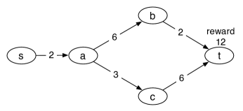
Figure 4: A minimal subgraph for motivating an agent to reach $t$.

Motivating subgraphs: A fundamental example. The basic set-up we consider is the following. Suppose the agent in the reward model is trying to construct a path from $s$ to $t$ in $G$; the reward $r$ is not under our control — perhaps it is defined by a third party, or represents an intrinsic reward that we cannot augment — but we are able to remove nodes and edges from the graph (essentially by declaring certain activities invalid, as the deadline did in Figure 2(b)). Let us say that a subgraph $G^{\prime}$ of $G$ motivates the agent if in $G^{\prime}$ with reward $r$, the agent reaches the goal node $t$. (We will also refer to $G^{\prime}$ as a motivating subgraph.) Note that it is possible for the full graph $G$ to be a motivating subgraph (of itself).

It would be natural to conjecture that if there is any subgraph $G^{\prime}$ of $G$ that motivates the agent, then there is a motivating subgraph consisting simply of an $s$-$t$ path $P$. Indeed, in any motivating subgraph $G^{\prime}$, the actual sequence of nodes and edges the agent traverses does form an $s$-$t$ path $P$, and so one might suspect that this path $P$ on its own should also be motivating.

In fact this is not the case, however. Figure 4 shows a graph illustrating a phenomenon that we find somewhat surprising a priori, though not hard to verify from the example. In the graph $G$ depicted in the figure, an agent with $\beta=1/2$ will reach the goal $t$. However, there is no proper subgraph of $G$ in which the agent will reach the goal. The point is that the agent starts out expecting to follow the path $s$-$a$-$b$-$t$, but when it gets to node $a$ it finds the remainder of the path $a$-$b$-$t$ too expensive to justify the reward, and it switches to $a$-$c$-$t$ for remainder. With just the path $s$-$a$-$b$-$t$ in isolation, the agent would get stuck at $a$; and with just $s$-$a$-$c$-$t$, the agent would never start out from $s$. It is crucial that the agent mistakenly believe the upper path is an option in order to eventually use the lower path to reach the goal.

It is interesting, of course, to consider real-life analogues of this phenomenon. In some settings, the structure in Figure 4 could correspond to deceptive practices on the part of the designer of $G$ — in other words, inducing the agent to reach the goal by misleading them at the outset. But there are other settings in real life where one could argue that the type of deception represented here is more subtle, not any one party’s responsibility, and potentially even salutary. For example, suppose the graph schematically represents the learning of a skill such as a musical instrument. There’s the initial commitment corresponding to the edge $(s,a)$, and then the fork at $a$ where one needs to decide whether to “get serious about it” (taking the expensive edge $(a,b)$) or not (taking the cheaper edge $(a,c)$). In this case, the agent’s trajectory could describe the story of someone who derived personal value from learning the violin (the lower path) even though at the outset they believed incorrectly that they’d be willing to put the work into becoming a concert violinist (the upper path, with the edge $(a,b)$ that proved too costly once the agent was standing at $a$).

The Structure of Minimal Motivating Subgraphs. Given that there is sometimes no single path in $G$ that is motivating, how rich a subgraph do we necessarily need to motivate the agent? Let us say that a subgraph $G^{*}$ of $G$ is a minimal motivating subgraph if (i) $G^{*}$ is motivating, and (ii) no proper subgraph of $G^{*}$ is motivating. Thus, for example, in Figure 4, the graph $G$ is a minimal motivating subgraph of itself; no proper subgraph of $G$ is motivating.

Concretely, then, we can ask the following question: what can a minimal motivating subgraph look like? For example, could it be arbitrarily dense with edges?

In fact, minimal motivating subgraphs necessarily have a sparse structure, which we now describe in our next theorem. To set up this result, we need the following definition. Given a directed acyclic graph $G$ and a path $P$ in $G$, we say that a path $Q$ in $G$ is a $P$-bypass if the first and last nodes of $Q$ lie on $P$, and no other nodes of $Q$ do; in other words, $P\cap Q$ is equal to the two ends of $Q$.

We now have

Theorem 5.1

If $G^{*}$ is a minimal motivating subgraph (from start node $s$ to goal node $t$), then it contains an $s$-$t$ path $P^{*}$ with the properties that

• Every edge of $G^{*}$ is either part of $P^{*}$ or lies on a $P^{*}$-bypass in $G^{*}$; and

• Every node of $G^{*}$ has at most one outgoing edge that does not lie on $P^{*}$ (in other words, $G^{*}-E(P^{*})$ has maximum out-degree $1$).

Proof:   If $G^{*}$ is a motivating subgraph, then the agent in $G^{*}$ will reach $t$. Consider the $s$-$t$ path the agent follows; we use this as the path $P^{*}$ in the theorem statement.

We first establish (i). Consider any edge $(v,w)$ of $G^{*}$ that is not on $P^{*}$. If there is a path $Q_{v}$ from $P^{*}$ to $v$, and a path $Q_{w}$ from $w$ to $P^{*}$, then $(v,w)$ must lie on a $P^{*}$-bypass, by simply concatenating the suffix of $Q_{v}$ from its last meeting with $P^{*}$, then the edge $(v,w)$, and then the prefix of $Q_{w}$ up to its first meeting with $P^{*}$.

So suppose by way of contradiction that $G^{*}$ contains an edge $(v,w)$ that does not belong to a $P^{*}$-bypass. Then it must be that there is either no path from $P^{*}$ to $v$, or no path from $w$ to $P^{*}$. In either case, for any node $u$ on $P^{*}$, there is no $u$-$t$ path that contains $(v,w)$. Thus the shortest-path evaluation of an agent standing at $u$ will not be affected if $(v,w)$ is deleted. Since the agent follows $P^{*}$ from $s$ to $t$, it must be that the agent would also do that in $G^{*}-\{(v,w)\}$, and this contradicts the minimality of $G^{*}$.

Now we consider property (ii). For any node $w$, we use $d^{*}(w,t)$ to denote the cost of a shortest $w$-$t$ path in $G^{*}$ (evaluated according to the true costs without present bias). Also, we fix a topological ordering of $G^{*}$. Suppose by way of contradiction that $(v,w)$ and $(v,w^{\prime})$ are both edges of $G^{*}$, where neither $w$ nor $w^{\prime}$ belongs to $P^{*}$. Let $Q_{w}^{*}$ and $Q_{w^{\prime}}^{*}$ denote shortest $w$-$t$ and $w^{\prime}$-$t$ paths respectively. Suppose (swapping the names of $w$ and $w^{\prime}$ if necessary) that $c(v,w)+d^{*}(w,t)\leq c(v,w^{\prime})+d^{*}(w^{\prime},t)$. Moreover, in the event the two sides of this inequality are equal, we assume the agent uses a consistent tie-breaking rule, so that if it is ever indifferent between using the edge $(v,w)$ or $(v,w^{\prime})$, it chooses $(v,w)$.

We claim that $G^{*}-\{v,w^{\prime}\}$ is a motivating subgraph, which will contradict the minimality of $G^{*}$. To see why, consider any node $p\in P^{*}$ that precedes $v$ in the chosen topological ordering and from which the agent’s planned path contains $v$. We consider two cases: if $p\neq v$, or if $p=v$. If $p\neq v$, then the planned path cannot contain the edge $(v,w^{\prime})$, since $(v,w)$ followed by $Q_{w}^{*}$ is no more expensive than $(v,w^{\prime})$ followed by $Q_{w^{\prime}}^{*}$, and if they are equal then we have established that the agent breaks ties in favor of $(v,w)$ over $(v,w^{\prime})$. If $p=v$, then the planned path also cannot contain the edge $(v,w^{\prime})$, since the planned path’s next edge lies on $P^{*}$, while $(v,w^{\prime})$ is not on $P^{*}$.

Thus there is no node from which the agent’s planned path contains the edge $(v,w^{\prime})$. Finally, we argue the agent will make the same sequence of decisions in $G^{*}-\{(v,w^{\prime})\}$ and $G^{*}$. Indeed, suppose there were a node where the agent made a different decision, and let $p\in P^{*}$ be the first such node. In $G^{*}$, the agent’s decision at $p$ is to follow the edge $(p,q)$ on $P^{*}$, as part of a planned path $R_{p}$. In $G^{*}-\{v,w^{\prime}\}$ the agent won’t decide to quit: the path $R_{p}$ is still available, since it does not contain $(v,w^{\prime})$. And in $G^{*}-\{v,w^{\prime}\}$, the agent can’t now prefer a path $R_{p}^{\prime}$ to $R_{p}$, since both $R_{p}$ and $R_{p}^{\prime}$ were available in $G^{*}$ as well, and the agent preferred $R_{p}$. Thus the agent makes the same sequence of decisions in $G^{*}-\{(v,w^{\prime})\}$ and $G^{*}$, and so $G^{*}-\{v,w^{\prime}\}$ is a motivating subgraph.      

6 Further Directions: Designing for Heterogeneous Agents

In the previous section we considered a set of questions that have a design flavor — how do we structure a graph to motivate an agent to reach the goal? A further general direction along these lines is to consider analogous questions for a collection of heterogeneous agents with different levels of present bias $\beta$.

In particular, suppose we have a population of agents, each with its own value of $\beta$, and we would like to design a structure in which as many of them as possible reach the goal. Or, adding a further objective, we may want many of them to reach the goal while minimizing the amount of (wasted) work done by agents who make partial progress but then fail to reach the goal.

This is a broad question that we pose primarily as a direction for further work. In particular, it is an interesting open question to explore the case of motivating subgraphs in the style of the previous section when there is not just one agent but a population of agents with heterogeneous values of $\beta$. To illustrate some of the considerations that arise, we give a tight analysis of a problem with heterogeneous agents in a model that is structurally much simpler than our graph-theoretic formulation.

Partitioning a Task for a Heterogeneous Population. The design question we consider is to divide up a single task into $k$ pieces so as to make it easier to motivate an agent to perform it. This is different from the setting of our graph model, in which tasks were indivisible and hence the splitting of a task wasn’t part of the set of design options. As we will see, even the problem of dividing a single task already contains some subtlety, and it lets us think about the relationships between agents with different levels of present bias.

We model our population of agents as a continuum, with $\beta$ uniformly distributed over $[0,1]$. Thus, rather than talking about the number of agents from a finite set who complete the task, we will think about the fraction that complete it.

Thus, suppose we have a task of cost $c$ and reward $r$, and it will be performed by a continuum of agents with $\beta$ uniformly distributed over $[0,1]$. We are allowed to partition the task into $k$ steps, of costs $c_{1},\ldots,c_{k}$, so that $c=\sum_{i=1}^{k}c_{i}$. Any partition has a completion rate, defined to be the fraction of agents who complete all the steps of the task. Our goal is to find a partition with maximum completion rate.

We define one additional piece of terminology: for any step in the decomposition of the task, the bottleneck value of the step is the minimum $\beta$ for which an agent of present bias $\beta$ will complete that step (when they evaluate the future steps and the reward as well using their parameter $\beta$).

Let us start by considering some small values of $k$, and then consider the general case.

${\bf k=1}$. When $k=1$, there is no choice in how to partition, since we just have a single step of cost $c$. In this case, the agents that perform the task are those for whom $c\leq\beta r$, and hence $\beta\geq c/r$. In other words, the bottleneck value of $\beta$ is $c/r$. We write $\gamma$ for this quantity $c/r$; in terms of $\gamma$, the completion rate is thus $1-\gamma$.

${\bf k=2}$. When $k=2$, we must divide the task into two steps so that the cost of the first step is some $x\in[0,c]$, and the cost of the second step is $c-x$. In this case, the bottleneck of the second step is $(c-x)/r$, and the bottleneck of the first step is the value $\beta$ such that $x+\beta(c-x)=\beta r$, which implies $\beta=\dfrac{x}{x+r-c}.$ We write $\delta=r-c$, and so we have the bottleneck $\beta=\dfrac{x}{x+\delta}.$

Now, the first bottleneck is monotone increasing in $x$, and the second bottleneck is monotone decreasing in $x$. We need to choose $x$ to minimize the larger of the two bottlenecks, which occurs when they are equal. Hence

$$\frac{c-x}{r} = \frac{x}{x+\delta}$$

from which we can solve for $x$ to get $x=\sqrt{\delta r}-\delta$. With this choice of $x$, the bottleneck of the two steps is the same; it is

$$\frac{x}{x+\delta}=1-\frac{\delta}{x+\delta}=1-\frac{\delta}{\sqrt{\delta r}}=1-\sqrt{\frac{\delta}{r}}=1-\sqrt{\frac{r-c}{r}}=1-\sqrt{1-\gamma},$$

and so the completion rate is $\sqrt{1-\gamma}$.

Arbitrary values of $k$. For a fixed value of $r$, let $f_{k}(c)$ denote the maximum completion rate of a task of cost $c$ and reward $r$, when we can partition it optimally into $k$ steps. Let $x_{k}^{*}(c)$ denote the cost of the first step in the optimal solution.

We claim by induction that

$$f_{k}(c)=(1-\gamma)^{1/k}$$

and

$$x_{k}^{*}(c)=\delta^{(k-1)/k}r^{1/k}-\delta,$$

and moreover that in the optimal solution the bottlenecks of all steps are the same, and equal to $1-f_{k}(c)$. Note that we have already established the case $k=2$ above.

For $k>2$, suppose we give the first step a cost of $x$. Then the bottleneck for the first step is, as before, $x/(x+\delta)$. The induction hypothesis tells us that the bottleneck for each of the remaining steps is

$$1-f_{k-1}(c-x)=1-\left(1-\frac{c-x}{r}\right)^{1/(k-1)}=1-\left(\frac{x+\delta}{r}\right)^{1/(k-1)}.$$

As in the case $k=2$, the bottleneck in the first step is monotone increasing in $x$, and the shared bottleneck in the remaining steps is monotone decreasing in $x$. Thus to minimize the largest bottleneck, we set the first bottleneck equal to the shared bottleneck in the remaining steps, obtaining

$$\frac{x}{x+\delta} = 1-\left(\frac{x+\delta}{r}\right)^{1/(k-1)}$$

and hence by solving for $x$, we get $x=\delta^{(k-1)/k}r^{1/k}-\delta$. With this value of $x$, we get a shared bottleneck of

$$\frac{x}{x+\delta}=1-\frac{\delta}{x+\delta}=1-\frac{\delta}{\delta^{(k-1)/k}r^{1/k}}=1-\left(\frac{\delta}{r}\right)^{1/k}=1-\left(\frac{r-c}{r}\right)^{1/k}=1-(1-\gamma)^{1/k},$$

which completes the induction step.

Note also that there is no wasted effort in this solution: since all the bottlenecks are the same, any agent who performs the first task will perform the remaining $k-1$ tasks as well. Thus no agents get partway through the sequence of tasks and then quit.

7 Conclusion and Open Questions

We have developed a graph-theoretic model in which an agent constructs a path from a start node $s$ to a goal node $t$ in an underlying graph $G$ representing a sequence of tasks. Time-inconsistent agents may plan an $s$-$t$ path that is different from the one they actually follow, and this type of behavior in the model can reproduce a range of qualitative phenomena including procrastination, abandonment of long-range tasks, and the benefits of a reduced set of options. Our results provide characterizations for a set of basic structures in this model, including for graphs achieving the highest cost ratios between time-inconsistent agents and shortest paths, and we have investigated the structure of minimal graphs on which an agent is motivated to reach the goal node.

There are many specific open questions suggested by this work, as well as more general directions for future research. We begin by mentioning three concrete questions.

1. Our graph-minor characterization in terms of the $k$-fan ${\cal F}_{k}$ is useful for instances with very large cost ratios. But this same graph minor structure may be useful for constant cost ratios as well. In particular, is there a function $f(\cdot)$ such that for all $k\geq 1$, any instance $G$ in which the undirected skeleton $\sigma(G)$ contains no ${\cal F}_{k}$ minor must have cost ratio at most $f(k)$?

2. We have investigated the structure of minimal motivating subgraphs. But how hard is it computationally to find motivating subgraphs? Is there a polynomial-time algorithm that takes an instance $G$ (including a reward $r$) and determines whether $G$ contains a motivating subgraph with reward $r$?

3. The definition of a motivating subgraph is based on a scenario in which a designer can delete nodes and/or edges from the task graph to make the goal $t$ easier to reach. An alternate way to motivate an agent to reach $t$ is to place intermediate rewards on specific nodes or edges; the agent will claim each reward if it reaches the node or edge on which it is placed. Now the question is to place rewards on the nodes or edges of an instance $G$ such that the agent reaches the goal $t$ while claiming as little total reward as possible; this corresponds to the designer’s objective to pay out as little as possible while still motivating the agent to reach the goal.

   There are a couple of points to note in this type of question about intermediate rewards. First, one should think about the implication for creating “exploitive” solutions in which the agent is motivated by intermediate rewards that it will never claim, because these rewards are on nodes that the agent will never reach. One could imagine a version of the problem, for example, in which rewards may only be placed on nodes or edges that the agent will actually traverse in the resulting solution. A second issue is the option of using negative rewards as well as positive ones; a negative reward could correspond to a step in which the agent has to “pay into the system” with the intention of receiving counterbalancing positive rewards at later points in the traversal of $G$. Note that there is a connection between negative rewards and questions involving motivating subgraphs: by placing a sufficiently large negative reward on a particular node or edge, it is possible to ensure that the agent won’t traverse it, and hence we can use negative intermediate rewards to implement the deletion of nodes and edges.

Beyond these specific questions, there is also a wide range of broader issues for further work. These include finding structural properties beyond our graph-minor characterization that have a bearing on the cost ratio of a given instance; obtaining a deeper understanding of the relationship between agents with different levels of time-inconsistency as measured by different values of $\beta$; and developing algorithms for designing graph structures that motivate effort as efficiently as possible, including for the case of multiple agents with diverse time-inconsistency properties.

Acknowledgments. We thank Supreet Kaur, Sendhil Mullainathan, and Ted O’Donoghue for valuable discussions and suggestions.

References

- [1] George A. Akerlof. Procrastination and obedience. American Economic Review: Papers and Proceedings, 81(2):1–19, May 1991.
- [2] Daniel Ariely and Klaus Wertenbroch. Procrastination, deadlines, and performance: self-control by precommitment. Psychological Science, 13(3):219–224, May 2002.
- [3] P. Carstensen. The complexity of some problems in parametric linear and combinatorial programming. PhD thesis, U. Michigan, 1983.
- [4] Reinhard Diestel. Graph Theory. Springer, 3 edition, 2005.
- [5] Herbert Edelsbrunner. Algorithms in Combinatorial Geometry. Springer, 1987.
- [6] Shane Frederick, George Loewenstein, and Ted O’Donoghue. Time discounting and time preference. Journal of Economic Literature, 40(2):351–401, June 2002.
- [7] Supreet Kaur, Michael Kremer, and Sendhil Mullainathan. Self-control and the development of work arrangements. American Economic Review: Papers and Proceedings, 100(2):624–628, 2010.
- [8] David Laibson. Golden eggs and hyperbolic discounting. Quarterly Journal of Economics, 112(2):443–478, 1997.
- [9] Evdokia Nikolova, Jonathan A. Kelner, Matthew Brand, and Michael Mitzenmacher. Stochastic shortest paths via quasi-convex maximization. In Proc. 14th European Symposium on Algorithms, pages 552–563, 2006.
- [10] Ted O’Donoghue and Matthew Rabin. Doing it now or later. American Economic Review, 89(1):103–124, March 1999.
- [11] Ted O’Donoghue and Matthew Rabin. Procrastination on long-term projects. Journal of Economic Behavior and Organization, 66(2):161–175, May 2008.
- [12] R. A. Pollak. Consistent planning. Review of Economic Studies, 35(2):201–208, April 1968.
- [13] Stuart L. Russell and Peter Norvig. Artificial Intelligence: A Modern Approach. Prentice Hall, 1994.
- [14] R. H. Strotz. Myopia and inconsistency in dynamic utility maximization. Review of Economic Studies, 23(3):165–180, 1955.