New tight approximations for Fisher’s exact test

Abstract

Fisher’s exact test is often a preferred method to estimate the significance of statistical dependence. However, in large data sets the test is usually too worksome to be applied, especially in an exhaustive search (data mining). The traditional solution is to approximate the significance with the $\chi^{2}$-measure, but the accuracy is often unacceptable. As a solution, we introduce a family of upper bounds, which are fast to calculate and approximate Fisher’s $p$-value accurately. In addition, the new approximations are not sensitive to the data size, distribution, or smallest expected counts like the $\chi^{2}$-based approximation. According to both theoretical and experimental analysis, the new approximations produce accurate results for all sufficiently strong dependencies. The basic form of the approximation can fail with weak dependencies, but the general form of the upper bounds can be adjusted to be arbitrarily accurate.

Keywords: Fisher’s exact test Upper bound Approximation Dependency rule

1 Introduction

Pattern recognition algorithms often involve testing the significance of a statistical dependency between two binary variables $X$ and $A$, given the observed counts $m(XA)$, $m(X\neg A)$, $m(\neg XA$, and $m(\neg X\neg A)$. If the test is done only a couple of times, the computation time is not crucial, but in an exhaustive search the test may repeated thousands or even millions of times.

For example, in data mining a classical problem is to search for the most significant classification rules of the form $X\rightarrow A$ or $X\rightarrow\neg A$, where $X$ is a set of binary attributes and $A$ is a binary class attribute. This problem is known to be $NP$-hard with common significance measures like the $\chi^{2}$-measure [MS00] and no polynomial time solutions are known. Even a more complex problem is to search for all sufficiently significant dependency rules, where the consequence attribute is not fixed (see e.g. [WH10]). In both problems the number of all tested patterns can be exponential and therefore each rule should be tested as fast as possible, preferrably in a constant time.

The problem is that typically the mined data sets are very large (the number of attributes can be tens of thousands and the number of rows millions). Still, the most significant (non-trivial) dependency rules may be relatively infrequent and the corresponding distributions too skewed for fast but inaccurate asymptotic tests. For accurate results, one should test the significance of dependency $X\rightarrow A$ with Fisher’s exact test, which evaluates the exact probability of the observed or a stronger dependency in the given data, if $X$ and $A$ were actually independent. For a positive dependency between $X$ and $A$ the probability ($p$-value) is defined by the cumulative hypergeometric distribution

$$p_{F}(X\rightarrow A)=\sum_{i=0}^{J}\frac{\left(m(X)\atop m(XA)+i\right)\left(m(\neg X)\atop m(\neg X\neg A)+i\right)}{\left(n\atop m(A)\right)},$$

where $m(Z)$ is the absolute frequency of set $Z$, $n$ is the data size (number of rows), and $J=\min\{m(X\neg A),m(\neg XA)\}$. (For a negative dependency between $X$ and $A$ it suffices to replace $A$ by $\neg A$.)

However, Fisher’s exact test is computationally demanding, when the data size $n$ is large. In each test one should evaluate $J+1\leq\frac{n}{4}+1$ terms, which means that the worst case time complexity is ${\mathcal{O}}(n)$. For example, if $m(X)=m(A)=500000$ and $m(XA)=300000$, we should evaluate 200 001 terms. In addition, each term involves binomial factors, but they can be evaluated in a constant time, if all factorials $i!$, $i=1,\ldots,n$ have been tabulated in the beginning.

A common solution is to estimate the $p$-values from the $\chi^{2}$-measure, when the data size is moderate or large. The justification is that asymptotically (when $n$ approaches $\infty$) $p_{F}$ can be approximated by the $\chi^{2}$-based $p$-values. However, in finite data sets the approximations are often quite inaccurate. The reason is that the $\chi^{2}$-measure is very sensitive to the data distribution. If the exact hypergeometric distribution is symmetric, the $\chi^{2}$-measure works well, but the more skewed the distribution is, the more inaccurate the approximated $p$-values are [Yat84, Agr92]. Classically [Fis25], it is recommended that the $\chi^{2}$-approximation should not be used, if any of the expected counts (under the assumption of independence between $X$ and $A$) $nP(X)P(A)$, $nP(X)P(\neg A)$, $nP(\neg X)P(A)$, or $nP(\neg X)P(\neg A)$ is less than 5. However, this rule of thumb prevents only the most extreme cases, which would lead to false discoveries. If the problem is to search for e.g. the best 100 dependency rules, the $\chi^{2}$-measure produces quite different results than $p_{F}$, even if all expected counts and the data size are large.

In this paper, we introduce better approximations for the exact $p_{F}$-values, which still can be calculated in a constant time. The approximations are upper bounds for the $p_{F}$ (when the $\chi^{2}$-based values are usually lower bounds, i.e. better than true values), but when the dependency is sufficiently strong, they give tight approximates to the exact values. In practice, they give identical results with the exact $p_{F}$-values, when used for rule ranking.

The idea of the approximations is to calculate only the first or a couple of first terms from $p_{F}$ exactly and estimate an upper bound for the rest terms. The simplest upper bound evaluates only the first term exactly. It is also intuitively the most appealing as a goodness measure, because it is reminiscent to the existing dependency measures like the odds ratio. When the dependencies are sufficiently strong (a typical data mining application), the results are also highly accurate. However, if the data set contains only weak and relatively insignificant dependencies, the simplest upper bound may produce too inaccurate results. In this case, we can use the tighter upper bounds, one of which can be adjusted to arbitrary accurate. However, the more accurate $p$-values we want to get, the more terms we have to calculate exactly. Fortunately, the largest terms of $p_{F}$ are always the first ones, and in practice it is sufficient to calculate only a small fraction (typically 2–10) of them exactly.

The rest of the paper is organized as follows. In Section 2 we introduce the upper bounds and give error bounds for the approximations. In Section 8 we evaluate the upper bounds experimentally, concentrating on the weak (and potentially the most problematic) dependencies. The final conclusions are drawn in Section 9.

Table 1: Basic notations.

$A$	a single binary attribute
$A\equiv(A=1)$	a short-hand notation for an event,
	where $A$ is true
$\neg A\equiv(A=0)$	a short-hand notation for an event,
	where $A$ is false
$X=\{A_{1},\ldots,A_{l}\}$	a set of binary attributes
$X\equiv(A_{1}=1\wedge\ldots A_{l}=1)$	a short-hand notation for an event,
	where all attributes $A_{i}\in X$, $|X|=l$,
	are true
$\neg X\equiv\neg(A_{1}=1\wedge\ldots A_{l}=1)$	a short-hand notation for an event,
	where $A_{i}=0$ for some $A_{i}\in X$
$n$	data size (number of rows)
$m(X)$	absolute frequency of $X$
$P(X)=\frac{m(X)}{n}$	relative frequency of $X$
$\delta(X,A)=P(XA)-P(X)P(A)$	leverage
$\gamma(X,A)=\frac{P(XA)}{P(X)P(A)}$	lift

2 Upper bounds

The following theorem gives two useful upper bounds, which can be used to approximate Fisher’s $p_{F}$. The first upper bound is more accurate, but it contains an exponent, which makes it more difficult to evaluate. The latter upper bound is always easy to evaluate and also intuitively appealing.

Theorem 3.

Let us notate $p_{F}=p_{0}+p_{1}+\ldots+p_{J}$ and $q_{i}=\frac{p_{i}}{p_{i-1}}$, $i\geq 1$. For positive dependency rule $X\rightarrow A$ with lift $\gamma(X,A)=\frac{p(XA)}{P(X)P(A)}$

$$p_{F} \leq p_{0}\left(\frac{1-q_{1}^{J+1}}{1-q_{1}}\right)$$

$$\leq p_{0}\left(1+\frac{1-P(A)\gamma(X,A)-P(X)\gamma(X,A)+P(X)P(A)\gamma(X,A)^{2}}{\gamma(X,A)-1}\right).$$

Proof.

Each $p_{i}$ can be expressed as $p_{i}=p_{abs}t_{i}$, where $p_{abs}=\frac{m(A)!m(\neg A)!}{n!}$ is constant. Therefore, it is enough to show the result for $p_{X}=\frac{p_{F}}{p_{abs}}$.

$p_{X}=t_{0}+t_{1}+...+t_{J}=t_{0}+q_{1}t_{0}+q_{1}q_{2}t_{0}+...+q_{1}q_{2}...q_{J}t_{0}$, where

$$q_{i} =\frac{t_{i}}{t_{i-1}}$$

$$=\frac{(m(XA)+i-1)!(m(\neg X\neg A)+i-1)!(m(X\neg A)-i+1)!(m(\neg XA)-i+1)!}{(m(XA)+i)!(m(\neg X\neg A)+i)!(m(X\neg A)-i)!(m(\neg XA)-i)!}=$$

$$=\frac{(m(X\neg A)-i+1)(m(\neg XA)-i+1)}{(m(XA)+i)(m(\neg X\neg A)+i)}.$$

Since $q_{i}$ decreases when $i$ increases, the largest value is $q_{1}$. We get an upper bound

$p_{X}=t_{0}+q_{1}t_{0}+q_{1}q_{2}t_{0}+...+q_{1}q_{2}...q_{J}t_{0}\leq t_{0}(1+q_{1}+q_{1}^{2}+q_{1}^{3}+...+q_{1}^{J}).$

The sum of geometric series is $t_{0}\frac{1-q_{1}^{J+1}}{1-q_{1}}$, which is the first upper bound. On the other hand,

$$t_{0}\frac{1-q_{1}^{J+1}}{1-q_{1}}\leq\frac{t_{0}}{1-q_{1}}=t_{0}(1+\frac{q_{1}}{1-q_{1}}).$$

Let us insert $q_{1}=\frac{m(X\neg A)m(\neg XA)}{(m(XA)+1)(m(\neg X\neg A)+1)}$, and express the frequencies using lift $\gamma=\gamma(X,A)$. For simplicity, we use notations $x=P(X)$ and $a=P(A)$. Now $m(XA)=nxa\gamma$, $m(X\neg A)=nx-nxa\gamma$, $m(\neg XA)=na-nxa\gamma$ and $m(\neg X\neg A)=n(1-x-a+xa\gamma)$. We get

$$\frac{q_{1}}{1-q_{1}} =\frac{m(X\neg A)m(\neg XA)}{(m(XA)+1)(m(\neg X\neg A)+1)-m(X\neg A)m(\neg XA)}$$

$$=\frac{n^{2}xa-n^{2}xa^{2}\gamma-n^{2}x^{2}a\gamma+n^{2}x^{2}a^{2}\gamma^{2}}{n^{2}xa\gamma+2nxa\gamma+n-nx-na+1-n^{2}xa}$$

$$=\frac{nxa-nxa^{2}\gamma-nx^{2}a\gamma+nx^{2}a^{2}\gamma^{2}}{nxa\gamma+2xa\gamma+1-x-a+1/n-nxa}$$

The nominator is $\geq nxa\gamma-nxa$, because $2xa\gamma+1-x-a+1/n\geq 0\Leftrightarrow$ $P(XA)+P(\neg X\neg A)+1/n\geq 0$. Therefore

$$\frac{q_{1}}{1-q_{1}}\leq\frac{1-a\gamma-x\gamma+xa\gamma^{2}}{\gamma-1}.$$

∎

In the following, we will denote the looser (simpler) upper bound by $ub1$ and the tighter upper bound (sum of the geometric series) by $ub2$. In $ub1$, the first term of $p_{F}$ is always exact and the rest are approximated, while in $ub2$, the first two terms are always exact and the rest are approximated.

We note that $ub1$ can be expressed equivalently as

$$ub1=p_{0}\left(\frac{P(XA)P(\neg X\neg A)}{\delta(X,A)}\right)=p_{0}\left(1+\frac{P(X\neg A)P(\neg XA)}{\delta(X,A)}\right),$$

where $\delta(X,A)=P(XA)-P(X)P(A)$ is the leverage. This is expression is closely related to the odds ratio

$$odds(X,A)=\frac{P(XA)P(\neg X\neg A)}{P(X\neg A)P(\neg XA)}=1+\frac{\delta}{P(X\neg A)P(\neg XA)},$$

which is often used to measure the strength of the dependency. The odds ratio can be expressed equivalently as

$$odds(X,A)=\frac{ub1}{ub1-1}.$$

We see that when the odds ratio increases (dependency becomes stronger), the upper bound decreases. In practice, it gives a tight approximation to Fisher’s $p_{F}$, when the dependency is sufficiently strong. The error is difficult to bind tightly, but the following theorem gives a loose upper bound for the error, when $ub2$ is used for approximation.

Theorem 4.

When $p_{F}$ is approximated by $ub2$, the error is bounded by

$$err\leq p_{0}\left(\frac{q_{1}^{2}}{1-q_{1}}\right).$$

Proof.

Upper bound $ub2$ can cause error only, if $J>1$. If $J=0$, $ub2=p_{0}$ and if $J=1$, $ub2=p_{0}\left(\frac{1-q_{1}^{2}}{1-q_{1}}\right)=p_{0}(1+q_{1})=p_{0}+p_{1}=p_{F}$. Let us now assume that $J>1$. The error is $err=ub2-p_{F}=p_{0}(1+q_{1}+\ldots+q_{1}^{J}-1-q_{1}-q_{1}q_{2}-\ldots-q_{1}q_{2}\ldots q_{J})=p_{0}(q_{1}^{2}+q_{1}^{3}+\ldots q_{1}^{J}-q_{1}q_{2}-\ldots-q_{1}q_{2}\ldots q_{J})$. It has an upper bound

$$err<p_{0}q_{1}^{2}(1+q_{1}+\ldots+q_{1}^{J-2})=p_{0}q_{1}^{2}\left(\frac{1-q_{1}^{J-1}}{1-q_{1}}\right)\leq p_{0}\left(\frac{q_{1}^{2}}{1-q_{1}}\right).$$

∎

This leads to the following corollary, which gives good guarantees for the safe use of $ub2$:

Corollary 5.

If $\gamma(X,A)\geq\frac{1+\sqrt{5}}{2}\approx 1.62$, then $err=ub2-p_{F}\leq p_{0}$.

Proof.

According to Theorem 4, $err\leq p_{0}$, if $q_{1}^{2}\leq 1-q_{1}$. This is true, when $q_{1}\leq\frac{\sqrt{5}-1}{2}$.

On the other hand, $q_{1}<\frac{1}{\gamma}$, when $\gamma>1$, because

$$q_{1}=\frac{m(X\neg A)m(\neg XA)}{(m(XA)+1)(m(\neg X\neg A)+1)}<\frac{P(X\neg A)P(\neg XA)}{P(XA)P(\neg X\neg A)}=\frac{xa(1-a\gamma)(1-x\gamma)}{xa\gamma(1-x-a+xa\gamma)}.$$

This is $\leq\frac{1}{\gamma}$, because $1-a\gamma-x\gamma+xa\gamma^{2}\leq 1-x-a+xa\gamma\Leftrightarrow 0\leq x(\gamma-1)+a(\gamma-1)-xa\gamma(\gamma-1)=(x+a-P(XA))(\gamma-1)$.

A sufficient condition for $q_{1}\leq\frac{\sqrt{5}-1}{2}$ is that

$$\frac{1}{\gamma}\leq\frac{\sqrt{5}-1}{2}\Leftrightarrow\gamma\geq\frac{2}{\sqrt{5}-1}=\frac{\sqrt{5}+1}{2}.$$

∎

This result also means that $ub2\leq 2p_{F}$, when the lift is as large as required.

The simpler upper bound, $ub1$, can cause a somewhat larger error than $ub2$, but it is even harder to analyze. However, we note that $ub1=p_{F}$ only, when $J=0$. When $J=1$, there is already some error, but in practice the difference is marginal. The following theorem gives guarantees for the accuracy of $ub1$, when $\gamma\geq 2$.

Theorem 6.

If $p_{F}$ is approximated with $ub1$ and $\gamma(X,A)\geq 2$, the error is bounded by $err\leq p_{0}$.

Proof.

The error is $err=ub1-p_{F}=ub1-ub2+ub2-p_{F}$, where $ub2-p_{F}\leq p_{0}\left(\frac{q_{1}^{2}}{1-q_{1}}\right)$ by Theorem 4.

When $\gamma\geq 2$, $ub1$ (being a decreasing function of $\gamma$) is

$$ub1=p_{0}\left(\frac{\gamma(1-a\gamma-x\gamma+xa\gamma^{2})}{\gamma-1}\right)\leq p_{0}2(1-a-x+2xa).$$

Therefore, the error is bounded by

$$err \leq p_{0}\left(2(1-a-x+2xa)-\frac{1-q_{1}^{J+1}}{1-q_{1}}+\frac{q_{1}^{2}}{1-q}\right)$$

$$=p_{0}\left(2-2a-2x+4xa-\frac{(1-q_{1}^{2}-q_{1}^{J+1})}{(1-q_{1})}\right)$$

$$=p_{0}\left(\frac{2(1-q_{1})-2a(1-q_{1})-2x(1-q_{1})+4xa(1-q_{1})-1+q_{1}^{2}+q_{1}^{J+1}}{1-q_{1}}\right)$$

$$=p_{0}\left(\frac{1-2q_{1}+q_{1}^{2}+q_{1}^{J+1}2a(1-q_{1})-2x(1-q_{1})+4xa(1-q_{1})}{1-q_{1}}\right).$$

When $\gamma\geq 2$, $q_{1}\leq\frac{1}{2}$, and thus

$$1-2q_{1}+q_{1}^{2}+q_{1}^{J+1} \leq 1-q_{1}\Leftrightarrow$$

$$0 \leq q_{1}-q_{1}^{2}-q_{1}^{J+1}\Leftrightarrow$$

$$0 \leq q_{1}(1-q_{1}-q_{1}^{J}).$$

Therefore,

$$err\leq p_{0}\left(\frac{(1-q_{1})(1-2a-2x+4xa)}{1-q_{1}}\right)=p_{0}(1-2a-2x+4xa).$$

The latter factor is always $\leq 1$, because $2a+2x-4xa=2a(1-x)+2x(1-a)\geq 0$. Therefore $err\leq p_{0}$. ∎

Our experimental results support the theoretical analysis, according to which both upper bounds, $ub1$ and $ub2$, give tight approximations to Fisher’s $p_{F}$, when the dependency is sufficiently strong. However, if the dependency is weak, we may need a more accurate approximation. A simple solution is to include more larger terms $p_{0}+p_{1}+\ldots p_{l-1}$ to the approximation and estimate an upper bound only for the smallest terms $p_{l}+\ldots p_{J}$ using the sum of the geometric series. The resulting approximation and the corresponding error bound are given in the following theorem. We omit the proofs, because they are essentially identical with the previous proofs for Theorems 3 and 4.

Theorem 7.

For positive dependency rule $X\rightarrow A$ holds

$$p_{F}\leq p_{0}+\ldots p_{l-1}+p_{l}\left(\frac{1-q_{l+1}^{J-l+1}}{1-q_{l+1}}\right),$$

where

$$q_{l+1}=\frac{(m(X\neg A)-l)(m(\neg XA)-l)}{(m(XA)+l+1)(m(\neg X\neg A)+l+1)}$$

and $l+1\leq J$.

The error of the approximation is

$$err\leq p_{0}\left(\frac{q_{l+1}^{2}}{1-q_{l+1}}\right).$$

8 Evaluation

Figure 1 shows the typical behaviour of the new upper bounds, when the strength of the dependency increases (i.e. $m(XA)$ increases and $m(X)$ and $m(A)$ remain unchanged). In addition to upper bounds $ub1$ and $ub2$, we consider a third upper bound, $ub3$, based on Theorem 7, where the first three terms of $p_{F}$ are evaluated exactly and the rest is approximated. All three upper bounds approach to each other and the exact $p_{F}$-value, when the dependency becomes stronger.

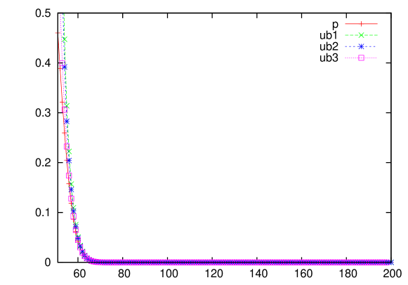
Figure 1: Exact $p_{F}$ and three upper bounds as functions of $m(XA)$, when $m(X)=200$, $m(A)=250$, and $n=1000$. The strength of the dependency increases on the $x$-axes.

Figure 2 shows a magnified area from Figure 1. In this area, the dependencies are weak, the upper bounds diverge from the exact $p_{F}$. The reason is that in this area the number of approximated terms is also the largest. For example, when $m(XA)=55$, $p_{F}$ contains 146 terms, and when $m(XA)=65$, it contains $136$ terms. In these points the lift is $1.1$ and $1.3$, respectively. The difference between $ub1$ and $ub2$ is marginal, but $ub3$ clearly improves $ub1$.

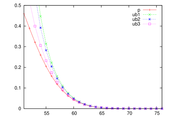
Figure 2: A magnified area from Figure 1 showing the differences, when the dependency is weak.

Because the new upper bound gives accurate approximations for strong dependencies, we evaluate the approximations only for the potentially problematic weak dependencies. As an example, we consider two data sets, where the data size is either $n=1000$ or $n=10000$. For both data sets, we have three test cases: 1) when $P(X)=P(A)=0.5$, 2) when $P(X)=0.2$ and $P(A)=0.25$, and 3) when $P(X)=0.05$ and $P(A)=0.2$. (The second case with $n=1000$ is shown in Figures 1 and 2.) For all test cases we have calculated the exact $p_{F}$, three versions of the upper bound $ub1$, $ub2$ and $ub3$, and the $p$-value achieved from the one-sided $\chi^{2}$-measure. The $\chi^{2}$-based $p$-values were calculated with an online Chi-Square Calculator [GS]. The values are reported for the cases, where $p_{F}\approx 0.05$, $p_{F}\approx 0.01$, and $p_{F}\approx 0.001$. Because the data is discrete, the exact $p_{F}$-values always deviate somewhat from the reference values.

The results for the first data set ($n=1000$) are given in Table 2 and for the second data set ($n=10000$) in Table 3. As expected, the $\chi^{2}$-approximation works best, when the data size is large and the distribution is balanced (case 1). According to the classical rule of a thumb, the $\chi^{2}$-approximation can be used, when all expected counts are $\geq 5$ [Fis25]. This requirement is not satisfied in the third case in the smaller data set. The resulting $\chi^{2}$-based $p$-values are also the least accurate, but the $\chi^{2}$-test produced inaccurate approximations also for the case 2, even if the smallest expected frequency was 50.

In the smaller data set, the $\chi^{2}$-approximation overperformed the new upper bounds only in the first case, when $p_{F}\approx 0.05$. If we had calculated the first four terms exactly, the resulting $ub4$ would have already produced a better approximation.

In the larger data set, $\chi^{2}$ gave more accurate results for the first two cases, when $p_{F}\approx 0.05$ and for the case 1, when $p_{F}\approx 0.01$. When $p_{F}\approx 0.001$, the new upper bounds gave always more accurate approximations. If we had calculated the first eight terms exactly, the resulting $ub8$ would have overperformed the $\chi^{2}$-approximation in case 1 with $p_{F}\approx 0.01$ and case 2 with $p_{F}\approx 0.05$. Calculating eight exact terms is quite reasonable compared to all 2442 terms, which have to be calculated for the exact $p_{F}$ in case 1. With 15 exact terms, the approximation for the case 1 with $p_{F}\approx 0.05$ would have also been more accurate than the $\chi^{2}$-based approximation. However, in so large data set (especially with an exhaustive search), a $p$-value of 0.05 (or even 0.01) is hardly significant. Therefore, we can conclude that for practical search purposes the new upper bounds give better approximations to the exact $p_{F}$ than the $\chi^{2}$.

Table 2: Comparison of the exact $p_{F}$ value, three upper bounds, and the $p$-value based on the $\chi^{2}$-measure, when $n=1000$. The best approximations are emphasized. $E(m(XA))$ is the expected frequency of $XA$ under the independence assumption.

1) $n=1000$, $m(X)=500$, $m(A)=500$, $E(m(XA))=250$
$m(XA)$	$p_{F}$	$ub1$	$ub2$	$ub3$	$p(\chi 2)$
263	0.0569	0.0696	0.0674	0.0617	0.050
269	0.0096	0.0107	0.0105	0.0100	0.0081
275	0.00096	0.00103	0.00101	0.00100	0.00080
2) $n=1000$, $m(X)=200$, $m(A)=250$, $E(m(XA))=50$
$m(XA)$	$p_{F}$	$ub1$	$ub2$	$ub3$	$p(\chi 2)$
60	0.0429	0.0508	0.0484	0.0447	0.0340
63	0.0123	0.0137	0.0132	0.0125	0.088
68	0.00089	0.00094	0.00092	0.00089	0.00050
3) $n=1000$, $m(X)=50$, $m(A)=200$, $E(m(XA))=1$
$m(XA)$	$p_{F}$	$ub1$	$ub2$	$ub3$	$p(\chi 2)$
15	0.0559	0.0655	0.0605	0.0565	0.0349
17	0.0123	0.0135	0.0128	0.0124	0.0056
19	0.00194	0.00205	0.00198	0.00194	0.00050

Table 3: Comparison of the exact $p_{F}$ value, three upper bounds, and the $p$-value based on the $\chi^{2}$-measure, when $n=10000$. The best approximations are emphasized. $E(m(XA))$ is the expected frequency of $XA$ under the independence assumption.

1) $n=10000$, $m(X)=5000$, $m(A)=5000$, $E(m(XA))=2500$
$m(XA)$	$p_{F}$	$ub1$	$ub2$	$ub3$	$p(\chi 2)$
2541	0.0526	0.0655	0.0647	0.0621	0.0505
2559	0.0096	0.0109	0.0109	0.0106	0.0091
2578	0.00097	0.00105	0.00104	0.00102	0.00090
2) $n=10000$, $m(X)=2000$, $m(A)=2500$, $E(m(XA))=500$
$m(XA)$	$p_{F}$	$ub1$	$ub2$	$ub3$	$p(\chi 2)$
529	0.0504	0.0623	0.0611	0.0579	0.047
541	0.0100	0.0113	0.0112	0.0108	0.0090
554	0.00109	0.00118	0.00116	0.00114	0.00090
3) $n=10000$, $m(X)=500$, $m(A)=2000$, $E(m(XA))=10$
$m(XA)$	$p_{F}$	$ub1$	$ub2$	$ub3$	$p(\chi 2)$
115	0.0498	0.0608	0.0583	0.0541	0.0427
121	0.0105	0.0118	0.0115	0.0109	0.0080
128	0.00106	0.00114	0.00112	0.00108	0.00070

9 Conclusions

We have introduced a family of upper bounds, which can be used to estimate Fisher’s $p_{F}$ accurately. Unlike the $\chi^{2}$-based approximations, these upper bounds are not sensitive to the data size, distribution, or small expected counts. In practical data mining purposes, the simplest upper bound produces already accurate results, but if all existing dependencies are weak and relatively insignificant, the results can be too inaccurate. In this case, we can use a general upper bound, whose accuracy can be adjusted freely. In practice, it is usually sufficient to calculate only a couple of terms from the Fisher’s $p_{F}$ exactly. In large data sets, this is an important concern, because the exact $p_{F}$ can easily require evaluation of thousands of terms for each tested dependency.

References

- [Agr92] A. Agresti. A survey of exact inference for contingency tables. Statistical Science, 7(1):131–153, 1992.
- [Cor09] H.J. Cordell. Detecting gene–gene interactions that underlie human diseases. Nature Reviews Genetics, 10:392–404, June 2009.
- [Fis25] R.A. Fisher. Statistical Methods for Research Workers. Oliver and Boyd, Edinburgh, 1925.
- [GS] Inc GraphPad Software. Quickcalcs online calculators for scientists. http://www.graphpad.com/quickcalcs/contingency1.cfm. Retrieved 18.5. 2010.
- [HRM03] L.W. Hahn, M.D. Ritchie, and J.H. Moore. Multifactor dimensionality reduction software for detecting gene–gene and gene–environment interactions. Bioinformatics, 19:376–382, 2003.
- [WH10] W. Hämäläinen: Efficient Search for Statistically Significant Dependency Rules in Binary Data. Ph.D. dissertation. Series of Publications A, Report A-2010-2 Department of Computer Science, University of Helsinki, Finland. 2010.
- [MAW10] J.H. Moore, F.W. Asselbergs, and S. M. Williams. Bioinformatics challenges for genome-wide association studies. Bioinformatics, 26(4):445–455, 2010.
- [MS00] S. Morishita and J. Sese: Transversing itemset lattices with statistical metric pruning. In Proceedings of the Nineteenth ACM SIGMOD-SIGACT-SIGART Symposium on Principles of Database Systems (PODS’00), pages 226–236, ACM Press 2000.
- [Yat84] F. Yates. Test of significance for 2 x 2 contingency tables. Journal of the Royal Statistical Society. Series A (General), 147(3):426–463, 1984.