Relations between stellar mass and electron temperature-based metallicity for star-forming galaxies in a wide mass range ^∗

Abstract

We select 947 star-forming galaxies from SDSS-DR7 with [O iii]$\lambda$4363 emission lines detected at a signal-to-noise ratio larger than 5$\sigma$. Their electron temperatures and direct oxygen abundances are then determined. We compare the results from different methods. $t_{2}$, the electron temperature in the low ionization region, estimated from $t_{3}$, that in the high ionization region, is compared using three analysis relations between $t_{2}-t_{3}$. These show obvious differences, which result in some different ionic oxygen abundances. The results of $t_{3}$, $t_{2}$, $\rm O^{++}$/$\rm H^{+}$ and $\rm O^{+}$/$\rm H^{+}$ derived by using methods from IRAF and literature are also compared. The ionic abundances $\rm O^{++}$/$\rm H^{+}$ are higher than $\rm O^{+}$/$\rm H^{+}$ for most cases. The different oxygen abundances derived from $T_{\rm e}$ and the strong-line ratios show a clear discrepancy, which is more obvious following increasing stellar mass and strong-line ratio $R_{23}$. The sample of galaxies from SDSS with detected [O iii]$\lambda$4363 have lower metallicites and higher star formation rates, so they may not be typical representatives of the whole population of galaxies. Adopting data objects from Andrews & Martini, Liang et al. and Lee et al. data, we derive new relations of stellar mass and metallicity for star-forming galaxies in a much wider stellar mass range: from $10^{6}\,M_{\odot}$ to $10^{11}\,M_{\odot}$.

1 Introduction

Stellar mass and metallicity are two of the most fundamental physical properties of galaxies. Stellar mass reflects the amount of gas locked up in stars, while metallicity represents the gas reprocessed by stars and any exchange of gas between the galaxy and its environment (Tremonti et al. 2004).

To estimate accurate values of metallicity for the ionized gas in galaxies, the electron temperature ($T_{\rm e}$) in the gas is generally required, which is usually obtained from the ratio of auroral to nebular line intensities, such as [O iii]$\lambda\lambda$4959, 5007/[O iii]$\lambda$4363. This is generally known as the “direct $T_{\rm e}$-method” since $T_{\rm e}$ can be directly inferred from observed line ratios. However, it is well known that this procedure is difficult to carry out for metal-rich galaxies since, as the metallicity increases, the electron temperature decreases (as the cooling is via metal lines), and the auroral lines eventually become too faint to measure. Instead, other strong nebular line ratios are required to estimate the oxygen abundances of metal-rich galaxies ($12+\log\rm(O/H)>8.5$) (Pagel et al. 1979; Tremonti et al. 2004; Liang et al. 2006; Kewley & Dopita 2002).

For estimating electron temperatures $T_{\rm e}$, and then the $T_{\rm e}$-derived oxygen abundances for galaxies, several methods have been given in the literature. In the first part of this work, we compare these different methods based on a large sample of good quality data from the Sloan Digital Sky Survey (SDSS). The SDSS survey provides a large sample of galaxies whose [O iii]$\lambda$4363 fluxes have been measured, and whose $T_{\rm e}$-based metallicities could be reliably estimated.

The stellar mass and metallicity relation (MZR) of galaxies is a fundamental relationship that represents the evolutionary history and the present properties of galaxies. Generally, the metallicities and stellar masses of galaxies increase with their evolutionary processes. Therefore, usually more massive galaxies are more metal rich (Tremonti et al. 2004; Liang et al. 2004, 2007; Kewley & Ellison 2008, and the references therein). [Tremonti et al.(2004)Tremonti, Heckman, Kauffmann et al.] gave the origin of the mass metallicity relation from 53 000 star-forming galaxies in the SDSS. Several works have been trying to obtain the MZR from $T_{\rm e}$-based oxygen abundances.

However, for metal-rich galaxies, it is difficult to obtain their [O iii]4363 and then $T_{\rm e}$-based oxygen abundances, so the common method used is to rely on strong emission line ratios (the so called strong-line method) to estimate their metallicities. Some researchers have also tried to stack the spectra of multiple galaxies in given bins of stellar masses, and then derive their [O ii]$\lambda\lambda$7320, 7330 and $T_{\rm e}$-based oxygen abundances (Liang et al. 2007; Andrews & Martini 2013). However, the range of stellar masses is generally not wide. Therefore, in the second part of this work, we gather data from literature to build a sample with a wide range of stellar mass from 10${}^{6}~{}M_{\odot}$ to 10${}^{11}~{}M_{\odot}$. These data have been used to obtain $T_{\rm e}$ and $T_{\rm e}$-based oxygen abundances. Then we derive a relation of stellar mass and metallicity for galaxies in this wide range of stellar masses. These sample galaxies are taken from [Liang et al.(2007)Liang, Hammer, Yin et al.], [Andrews & Martini(2013)] and [Lee et al.(2006)Lee, Skillman, Cannon et al.]. [Lee et al.(2006)Lee, Skillman, Cannon et al.] gave the mass-metallicity relation of galaxies at lower stellar mass. [Liang et al.(2007)Liang, Hammer, Yin et al.] and [Andrews & Martini(2013)] worked on more metal-rich galaxies from SDSS.

We always keep in mind the difference between the oxygen abundances obtained from the electronic temperature method ($T_{\rm e}$-method) and the strong line ratio method (so-called $R_{23}$). This issue is still in debate (Kennicutt et al. 2003; Liang et al. 2007; Stasinska 2005). We compare them by using the good quality data here.

This paper is organized as follows. The sample selection criteria are described in Section 2. The determinations of $T_{\rm e}$ from line ratios and oxygen abundances from $T_{\rm e}$ are presented and compared in Section 3 in detail. In Section 4, we fit the relations of stellar mass and metallicity in a wide mass range from the $T_{\rm e}$-based oxygen abundances. We summarize this work in Section 5.

2 Sample selection

We select 947 star-forming galaxies from the SDSS-Data Release 7 (DR7) main galaxy sample for which their [O iii]$\lambda$4363 emission lines can be measured at a signal-to-noise ratio above 5$\sigma$. This auroral line can help us to reliably derive the electron temperature $T_{\rm e}$, and then have a direct measure of oxygen abundances from $T_{\rm e}$. We also require that these galaxies have stellar mass estimates. These sample galaxies are selected as follows and their numbers during the selection process are shown in Table 1.

We download 927 552 galaxies from the SDSS-DR7 (Adelman-McCarthy et al 2006). Then we select the galaxies with redshifts 0.03$<z<$0.25 to ensure we cover the range from [O ii] to H$\alpha$ and [S ii] emission lines. [Tremonti et al.(2004)Tremonti, Heckman, Kauffmann et al.] also discussed the weak effect of aperture on estimated metallicities of the sample galaxies with $0.03<z<0.25$ and this was further discussed by [Kewley et al.(2005)Kewley, Jansen, & Geller]. Then 747 970 galaxies remain after this criterion is applied.

Following the works of [Yin et al.(2007)Yin, Liang, Hammer et al.], [Liang et al.(2006)Liang, Yin, Hammer et al.] and [Tremonti et al.(2004)Tremonti, Heckman, Kauffmann et al.], we further select objects displaying [O ii]$\lambda\lambda$3726, 3729, [O iii]$\lambda$5007, H$\beta$, H$\alpha$, [N ii]$\lambda 6583$ and [S ii]$\lambda\lambda 6717,6731$ emission lines, and H$\beta$, H$\alpha$, [N ii] and [S ii] emission lines with adequate signal to noise (S/N) ($>$5 $\sigma$). There are 274 197 galaxies matching the criteria.

Since we will use the $T_{\rm e}$-method to derive O/H abundances for the sample of galaxies (see Sect. 3 for details), we select the samples with the [O iii]$\lambda$4363 emission line detected at an S/N ratio greater than 5$\sigma$. Then 1843 galaxies (from 274 197) are selected from this criterion.

We select 1072 “star-forming galaxies” from the 1843 galaxies based on the BPT diagram, which have been identified following the selection criteria of the traditional line diagnostic diagram [N ii]/H$\alpha$ vs. [O iii]/H$\beta$ (Baldwin et al. 1981; Veilleux & Osterbrock 1987; Kewley et al. 2001; Kauffmann et al. 2003). These objects are plotted on the BPT diagram as shown in Figure 1.

Figure 1: A BPT (Baldwin et al.1981) diagram in which we plot the emission-line flux ratio [O iii]/H$\beta$ versus the ratio [N ii]/H$\alpha$ for the galaxies in our sample. The solid curve shows the demarcation between star-forming galaxies (lower left) and active galactic nuclei (upper right) defined by [Kauffmann et al.(2003)Kauffmann, Heckman, Tremonti et al.]. The dashed line comes from [Kewley et al.(2001)Kewley, Dopita, Sutherland, Heisler, & Trevena] for reference. Our sample includes 1072 star-forming galaxies according to this definition.

To compare our sample galaxies with the whole SDSS main galaxy sample in terms of their relation between star formation rate (SFR) and stellar masses as shown in Section 4.1, we also select 211 725 “star-forming galaxies” from 274 197 galaxies following the BPT diagram for those objects without [O iii]$\lambda$4363 measurements. This is taken as the comparison sample.

Finally, we obtain 947 star-forming galaxies (see Table 2 for examples) with metallicity estimates (from the strong-line method) and stellar mass estimates by the MPA/JHU group. A table listing the entire sample of galaxies is also provided in the electronic version of the article. The comparison sample consists of 193 468 galaxies with measured stellar masses derived from the compilation of 211 725 galaxies mentioned above.

Table 1: List of Detailed Criteria and Galaxy Numbers

Criteria	Number of Galaxies
Original downloaded data set	927 552
0.03$<z<$0.25	747 970
S/N$>$0, S/N$>$5$\sigma$	274 197
[O iii] $\lambda 4363>5\sigma$	1843
Star forming (BPT)	1072
Stellar mass $>$0	947

Table 2: An Example Listing of the Galaxies in Our Sample

Num	Plate-MJD-FiberID	RA-Dec	$t_{3}$ (104K)	$t_{2}$ (104K)	12+(O++/H+)	12+(O+/H+)	12+(O/H)Te	12+(O/H)Bay
(1)	(2)	(3)	(4)	(5)	(6)	(7)	(8)	(9)
1	266-51630-407	145.891$+$ 1.117	1.140$\pm$0.023	1.098$\pm$0.016	7.877$\pm$0.029	7.862$\pm$0.027	8.138$\pm$0.028	8.666
2	267-51608-421	147.597$+$ 0.708	1.313$\pm$0.099	1.219$\pm$0.069	8.041$\pm$0.110	7.422$\pm$0.107	8.053$\pm$0.109	8.787
3	270-51909-617	153.629$+$ 0.799	1.202$\pm$0.043	1.142$\pm$0.030	8.086$\pm$0.051	7.563$\pm$0.048	8.125$\pm$0.051	8.396
4	276-51909-490	163.427$+$ 0.163	1.238$\pm$0.022	1.167$\pm$0.015	7.950$\pm$0.024	7.777$\pm$0.023	8.127$\pm$0.023	8.249
5	277-51908-451	165.318$+$ 0.804	1.525$\pm$0.123	1.367$\pm$0.086	7.968$\pm$0.105	6.983$\pm$0.109	7.913$\pm$0.105	8.000
6	280-51612-192	170.438$-$ 0.023	1.198$\pm$0.064	1.138$\pm$0.045	8.148$\pm$0.079	7.620$\pm$0.075	8.185$\pm$0.078	8.171
7	281-51614-129	172.003$-$ 1.127	1.189$\pm$0.045	1.132$\pm$0.032	8.096$\pm$0.054	7.667$\pm$0.051	8.164$\pm$0.054	8.047
8	282-51630-546	174.266$+$ 0.471	1.162$\pm$0.034	1.113$\pm$0.024	8.234$\pm$0.042	7.639$\pm$0.039	8.253$\pm$0.042	8.191
9	282-51658-543	174.266$+$ 0.471	1.245$\pm$0.064	1.171$\pm$0.045	8.140$\pm$0.073	7.579$\pm$0.070	8.168$\pm$0.073	8.188
10	283-51959-572	176.706$+$ 0.896	1.651$\pm$0.244	1.456$\pm$0.171	7.894$\pm$0.215	6.858$\pm$0.225	7.832$\pm$0.215	7.976

Notes: The sequence number, ID number in SDSS and the coordinates are listed in Cols. 1–3. The electron temperature $t_{3}$, $t_{2}$ from temden.nebular and oxygen abundances $\rm O^{++}$/$\rm H^{+}$ and O⁺/$\rm H^{+}$ from ionic.nebular are listed in Cols. 4–7. $t_{2}$ is calculated from $t_{3}$ with the equation $t_{2}=0.7t_{3}+0.3$. 12+(O/H)_Bay, obtained by the MPA/JHU group, and is listed in last column. The entire table of galaxies in our sample is provided in the electronic version.

In Section 3, we will use the sample of 947 galaxies to compare the different methods to estimate $T_{\rm e}$ and then oxygen abundances.

For the second part of this work presented in Section 4, we will study the stellar mass and metallicity relations of galaxies, and derive new relations from galaxies in a wide range of stellar masses. Therefore, we will also collect data with $T_{\rm e}$ and $T_{\rm e}$-based oxygen abundance estimates from literature: 30 data points from [Andrews & Martini(2013)] and 27 data points from [Liang et al.(2007)Liang, Hammer, Yin et al.] for higher stellar mass and higher metallicities, and 25 data points from [Lee et al.(2006)Lee, Skillman, Cannon et al.] for lower mass and lower metallicities. The former two are the stacked spectra of SDSS galaxies in each of the different stellar mass bins. More details will be discussed in Section 4.

3 Calculating electron temperature $T_{\rm e}$ and $T_{\rm e}$-based oxygen abundances for galaxies in the sample

3.1 Comparing Electron Temperatures from Different Methods

A two-zone model for the temperature structure within the H ii region was adopted (also see Yin et al. 2007). In this model, $T_{\rm e}$([O iii]) is taken to represent the temperature for high ionization species such as $\rm O^{++}$, while $T_{\rm e}$([O ii]) is used for low ionization species such as $\rm O^{+}$.

In principle, the temperature in the high ionization region $t_{3}$ ($=10^{-4}\,T_{\rm e}$ ([O iii])) can be derived from the emission line ratio of [O iii]$\lambda\lambda$4959, 5007/[O iii]$\lambda$4363, while the temperature in the low ionization region $t_{2}$ ($=10^{-4}T_{\rm e}$ ([O ii])) can be estimated from [O ii]$\lambda\lambda$7320, 7330/[O ii]$\lambda$3727 and [N ii]$\lambda$6548, 6583/[N ii]$\lambda$5755. But in the spectra, it is often difficult to detect the weak [O ii] and [N ii] lines except in some H ii regions (Kennicutt et al. 2003, Bresolin et al. 2004) and the stacked spectra of galaxies (Liang et al. 2007, Andrews & Martini 2013). [O iii]$\lambda$4363 is more commonly detected in metal-poor H ii regions and star forming galaxies. Thus, the common method is first deriving temperature $t_{3}$ from [O iii]$\lambda\lambda$4959, 5007/[O iii]$\lambda$4363 and then estimating $t_{2}$ from an analytical relation between $t_{2}$ and $t_{3}$ inferred from photoionization calculations.

The electron densities $n_{\rm e}$ in the ionized gas of the galaxies can be calculated at $T_{\rm e}=10\,000$ K from the line ratios [S ii]$\lambda 6717$/[S ii]$\lambda 6731$ by using the five-level statistical equilibrium model in the task temden.nebular contained in the iraf/stsdas package (de Robertis, Dufour & Hunt 1987; Shaw & Dufour 1995), which uses the latest atomic data. We adopt this method to calculate $n_{\rm e}$.

3.1.1 Comparing $t_{3}$ from different methods

The electron temperature $t_{3}$ (in units of $10^{4}$ K) can be estimated from the iterative formula given by [Izotov et al.(2006)Izotov, Stasińska, Meynet, Guseva, & Thuan], which was taken from [Aller(1984)]

$$t_{3}=\frac{1.432}{\log((\lambda 4959+\lambda 5007)/\lambda 4363)-\log C_{\rm T}}\,,$$ (1)

where

$$C_{\rm T}=\Big{(}8.44-1.09t_{3}+0.5t_{3}^{2}-0.08t_{3}^{3}\Big{)}\frac{1+0.0004x_{3}}{1+0.044x_{3}}\,,$$ (2)

with $x_{3}=10^{-4}n_{\rm e}t_{3}^{-1/2}$, and $n_{\rm e}$ is the electron density in cm^-3. They used atomic data from the references listed in [Stasińska(2005)].

The electron temperature $t_{3}$ can also be estimated by using the task temden.nebular contained in the iraf/stsdas package. This procedure is based on the five-level atom program (de Robertis, Dufour & Hunt 1987; Shaw & Dufour 1995).

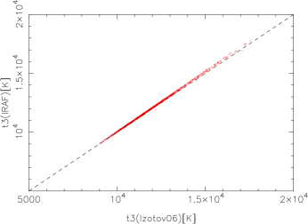
We compare these two sets of results for $t_{3}$, and get very similar results, which are shown in Figure 2. This means that these two methods from IRAF and the literature are quite similar. In the following studies, we will adopt the $t_{3}$ temperature estimated from temden.nebular in the iraf/stsdas package.

Figure 2: Comparing the $t_{3}$ temperatures estimated from the [Izotov et al.(2006)Izotov, Stasińska, Meynet, Guseva, & Thuan] formula with that from IRAF (temden.nebular). They are very similar in most parts. Only in the high-temperature range is $t_{3}$(IRAF) slightly larger. The average offset is 71.8 K from the equal-value line.

3.1.2 Comparing $t_{2}$ from different analysis formulae

To derive temperature $t_{2}$, similar to [Garnett(1992)], [Campbell et al.(1986)Campbell, Terlevich, & Melnick] used the photoionization models of [Stasińska(1982)] to derive a linear relation between $t_{2}$ and $t_{3}$

$$t_{2}=0.7t_{3}+0.3\,.$$ (3)

This is valid over the range 2000 ${\rm K}<T_{\rm e}$([O iii])$<18\,000~{}{\rm K}$, and has been widely used. [Pilyugin et al.(2010)Pilyugin, Vílchez, Cedrés, & Thuan] also derived a linear relation between $t_{2}-t_{3}$ as

$$t_{2}=0.835t_{3}+0.264\,.$$ (4)

They adopted the ff relation, and to convert the temperature indicator into the electron temperature value $t_{2}$, they used the five-level-atom solution of $\rm O^{+}$ with the Einstein coefficients for spontaneous transitions A_jk obtained by [Froese Fischer & Tachiev(2004)] and the effective cross sections for electron impact $\Omega_{jk}$ from [Pradhan et al.(2006)Pradhan, Montenegro, Nahar, & Eissner].

[Izotov et al.(2006)Izotov, Stasińska, Meynet, Guseva, & Thuan] also provide a set of analysis formulae to calculate $t_{2}$ from $t_{3}$ in three different ranges of metallicities: “low $Z$” refers to $12+\log({\rm O/H})<7.2$, “high $Z$” refers to $12+\log({\rm O/H})>8.2$ and “intermediate $Z$” refers to $7.2<12+\log({\rm O/H})<8.2$. Here we adopt their formulae for intermediate $Z$ and high $Z$ to estimate $t_{2}$, but do not consider the low $Z$ case. These sequences were defined as in [Stasińska & Izotov(2003)], but have been recomputed with the latest atomic data at that time, and with an input radiation field computed with Starburst 99 (Leitherer et al. 1999) using the stellar model atmospheres described in [Smith et al.(2002)Smith, Norris, & Crowther]

$$t_{2} =-0.744+t_{3}\times(2.338-0.610t_{3}), \quad{\rm intermed.\ }Z,$$ (5)

$$=2.967+t_{3}\times(-4.797+2.827t_{3}), \quad{\rm high\ }Z.$$

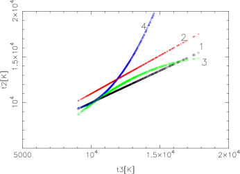
These three transition formulae (Eqs. (3), (4) and (5)) can be used to estimate $t_{2}$ from $t_{3}$. We would like to compare them by using the selected SDSS star-forming galaxies in this work, which have detected [O iii]$\lambda$4363 that have been used to estimate their electron temperature, $t_{3}$. The results clearly show the difference between the three sets of temperature $t_{2}$ in Figure 3, where Line-1 refers to the result from our Equation (3), Line-2 from Equation (4), Line-3 from the intermediate-$Z$ case of Equation (5) and Line-4 from its high-$Z$ case. Line-2 shows higher $t_{2}$ than Line-1 at a given $t_{3}$. Line-3 (the intermediate-$Z$ case of Eq. (5)) is close to Line-1 but it is not a linear relation. Line-4 shows much discrepancy compared to the other three lines except at the low temperature end. Thus we would not take Line-4 to estimate abundances in the later part of this work. We will estimate $\rm O^{+}$/$\rm H^{+}$ abundances of our sample galaxies by using the temperature $t_{2}$ shown by Lines-1, 2 and 3 in the next section.

We keep in mind that, as mentioned in [Andrews & Martini(2013)], the $t_{2}-t_{3}$ relation from our Equation (3) overestimates the low ionization zone $T_{\rm e}$[O ii] by $\sim$1000–2000 K and will underestimate the oxygen abundance by $\sim$0.18 dex. In this work, we cannot carefully check this result since by using the spectra of these individual objects, we cannot reliably estimate fluxes of their [O ii]$\lambda\lambda$7320,7330 auroral lines. However, in Section 3.4 we will discuss such effects on discrepancies in temperature and abundances following the suggestions of [Andrews & Martini(2013)].

Figure 3: Comparison of the $t_{2}$ temperature estimated from $t_{3}$ using the three transition formulae: Line-1 refers to the result from Eq. (3), Line-2 from Eq. (4), Line-3 from the intermediate-$Z$ case of Eq. (5) and Line-4 from its high-$Z$ case. The data points are the star-forming galaxies from SDSS whose $t_{3}$ values have been estimated from [O iii]$\lambda\lambda$4959, 5007/[O iii]$\lambda$4363 with IRAF.

3.2 Comparing the Ionic Abundances from Two Different Methods

The ionic oxygen abundances $\rm O^{+}$/$\rm H^{+}$ and $\rm O^{++}$/$\rm H^{+}$ can be estimated from the electron temperature $t_{2}$ and $t_{3}$ and the related emission line ratios, respectively. The total oxygen abundances in the ionized nebulae can be derived from the relation of the line ratios

$$\frac{\rm O}{\rm H}=\frac{\rm O^{+}}{\rm H^{+}}+\frac{\rm O^{++}}{\rm H^{+}}\,.$$ (6)

The contributions from other ions such as O³⁺ can be omitted since they are small. [Izotov et al.(2006)Izotov, Stasińska, Meynet, Guseva, & Thuan] have recently published a set of equations for the determination of the oxygen abundances in H ii regions for a five-level atom. They used the atomic data from the references listed in [Stasińska(2005)]. They show the ionic abundances $\rm O^{++}$/$\rm H^{+}$ and $\rm O^{+}$/$\rm H^{+}$ are estimated as follows:

$$12+\log(\rm O^{++}/\rm H^{+}) = \log(I_{\rm{[O}{III]\lambda 4959+\lambda 5007}}/I_{\rm H\beta})$$ (7)

$$+6.200+\frac{1.251}{t_{3}}-0.55\log t_{3}-0.014t_{3}\,,$$

$$12+\log(\rm O^{+}/\rm H^{+}) = \log(I_{\rm{[O}{\rm II]\lambda 3726+\lambda 3729}}/I_{\rm H\beta})+5.961$$ (8)

$$+\frac{1.676}{t_{2}}-0.40\log t_{2}-0.034t_{2}+\log(1+1.35x_{2})\,,$$

with $x_{2}=10^{-4}n_{\rm e}t_{2}^{-1/2}$, and $n_{\rm e}$ is the electron density in cm^-3.

The ionic abundances $\rm O^{++}$/$\rm H^{+}$ and $\rm O^{+}$/$\rm H^{+}$ can also be estimated by using the task ionic.nebular contained in the iraf/stsdas package. We compare the ionic abundances from these two methods.

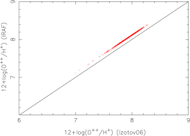
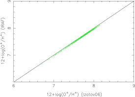
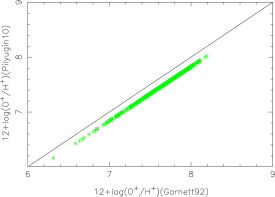
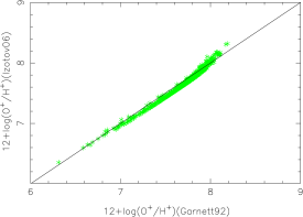
The $\rm O^{++}$/$\rm H^{+}$ abundances from ionic.nebular and [Izotov et al.(2006)Izotov, Stasińska, Meynet, Guseva, & Thuan] are compared in the left panel of Figure 4 ($t_{3}$ is calculated from temden.nebular). IRAF gives a slightly higher abundance, about 0.1 dex. The right panel of Figure 4 is for $\rm O^{+}$/$\rm H^{+}$ abundances; here we adopt $t_{2}=0.7t_{3}+0.3$ to estimate $t_{2}$, and then the derived $\rm O^{+}$/$\rm H^{+}$ abundances from ionic.nebular and [Izotov et al.(2006)Izotov, Stasińska, Meynet, Guseva, & Thuan] are also compared. These results show that the ionic abundances from the [Izotov et al.(2006)Izotov, Stasińska, Meynet, Guseva, & Thuan] formula are quite similar to those from the IRAF/IONIC procedure, and the average offset is 0.03 dex. The electronic temperatures and oxygen abundances of 947 sample galaxies are given in Table 2.

Figure 4: Left: Comparison of the $\rm O^{++}$/$\rm H^{+}$ abundances from ionic.nebular and [Izotov et al.(2006)Izotov, Stasińska, Meynet, Guseva, & Thuan] ($t_{3}$ from IRAF). We can see the abundances from ionic.nebular are slightly bigger. The average deviation is 0.11 dex from the equal-value line. Right: Comparison of the $\rm O^{+}$/$\rm H^{+}$ abundances from ionic.nebular and [Izotov et al.(2006)Izotov, Stasińska, Meynet, Guseva, & Thuan] ($t_{2}$ from Equation $t_{2}=0.7t_{3}+0.3$). The abundances are very similar for the two methods. The average deviation is 0.03 dex from the equal-value line.

3.3 Comparing the $\rm O^{+}$/$\rm H^{+}$ Abundances from Different $t_{2}$

Now we compare the $\rm O^{+}$/$\rm H^{+}$ abundances from the three different sets of $t_{2}$ from [Garnett(1992)] (Eq. (3)), [Pilyugin et al.(2010)Pilyugin, Vílchez, Cedrés, & Thuan] (Eq. (4)) and [Izotov et al.(2006)Izotov, Stasińska, Meynet, Guseva, & Thuan] (Eq. (5)).

The derived $\rm O^{+}$/$\rm H^{+}$ abundances are derived using the ionic.nebular procedure. The results are compared in Figure 5. The $\rm O^{+}$/$\rm H^{+}$ abundances from [Izotov et al.(2006)Izotov, Stasińska, Meynet, Guseva, & Thuan] are quite similar to the abundances from [Garnett(1992)], and the one from [Pilyugin et al.(2010)Pilyugin, Vílchez, Cedrés, & Thuan] will result in about 0.15 dex lower $12+\log\rm(O^{+}/H^{+})$ abundances than that of [Garnett(1992)].

Figure 5: Left: Comparison of the $\rm O^{+}$/$\rm H^{+}$ abundances with different $t_{2}$ formulae from [Garnett(1992)] (Eq. (3)) and [Pilyugin et al.(2010)Pilyugin, Vílchez, Cedrés, & Thuan] (Eq. (4)). The average residual is 0.15 dex. Right: Comparison of the $\rm O^{+}$/$\rm H^{+}$ abundances with different $t_{2}$ formulae from [Garnett(1992)] (Eq. (3)) and [Izotov et al.(2006)Izotov, Stasińska, Meynet, Guseva, & Thuan] (Eq. (5), intermediate-Z case). The average residual is 0.05 dex. The derived $\rm O^{+}$/$\rm H^{+}$ abundances are from ionic.nebular.

3.4 Comparing the $\rm O^{++}$/$\rm H^{+}$ and the $\rm O^{+}$/$\rm H^{+}$ Abundances

Now we compare the ionic abundances $\rm O^{++}$/$\rm H^{+}$ and $\rm O^{+}$/$\rm H^{+}$ in Figure 6 in the relation with stellar mass; here we adopt the $\rm O^{++}$/$\rm H^{+}$ and $\rm O^{+}$/$\rm H^{+}$ from ionic.nebular in IRAF and $t_{2}=0.7t_{3}+0.3$ for temperature $t_{2}$.

Figure 6 shows that for most cases $\rm O^{++}$/$\rm H^{+}$ is higher than $\rm O^{+}$/$\rm H^{+}$. We did not see the suggestions by [Andrews & Martini(2013)] that $\rm O^{+}$/$\rm H^{+}$ is more significant than $\rm O^{++}$/$\rm H^{+}$ (their fig. 5). Maybe that is because they are focusing on the massive galaxies. Another reason could be that we may underestimate the $\rm O^{+}/\rm H^{+}$ abundances since the analysis formula we used is $t_{2}=0.7t_{3}+0.3$ which overestimates $t_{2}$ as mentioned in [Andrews & Martini(2013)] (their fig. 5). This effect is shown in the lower right panel of Figure 6.

Figure 6: Upper left: Comparing the $\rm O^{++}$/$\rm H^{+}$ and $\rm O^{+}$/$\rm H^{+}$ abundances. Upper right: Showing the relations $\rm O^{++}$/$\rm H^{+}$ vs. stellar mass and $\rm O^{+}$/$\rm H^{+}$ vs. stellar mass. For comparison, we also plot the equal-value (8.0) line with a dashed line. Lower left: The relations of stellar mass vs. the residuals between $\rm O^{++}$/$\rm H^{+}$ and $\rm O^{+}$/$\rm H^{+}$. The average offset of the residuals is 0.36 dex from the zero-point line. Lower right: Similar relations of stellar mass vs. the residuals between $\rm O^{++}$/$\rm H^{+}$ and $\rm O^{+}$/$\rm H^{+}$, but the $\rm O^{+}$/$\rm H^{+}$ abundances have been artificially increased by 0.18 dex according to suggestions of [Andrews & Martini(2013)]. These plots show that O${}^{++}/\rm H^{+}$ is larger than $\rm O^{+}$/$\rm H^{+}$ for most galaxies. The values for electron temperature $t_{2}$ are estimated using the formula from [Garnett(1992)] (Eq. (3)). $\rm O^{++}$/$\rm H^{+}$ and $\rm O^{+}$/$\rm H^{+}$ oxygen abundances are calculated from ionic.nebular.

3.5 Comparing the Oxygen Abundances from the $T_{\rm e}$ Method and $R_{23}$ Method

We compare the difference between the oxygen abundances $12+\log$(O/H) obtained from the electronic temperature method ($T_{\rm e}$-method) and the strong emission-line ratio method (such $R_{23}$). This is shown in Figure 7.

We adopt the oxygen abundance based on the strong-line method obtained by the MPA/JHU group. The MPA/JHU group used a photoionization model to simultaneously fit most prominent emission lines. Based on a Bayesian technique, they have calculated the likelihood distribution of the metallicity of each galaxy in the sample by comparing with a large library of models corresponding to different assumptions about the effective gas parameters, and then they adopted the median of the distribution as the best estimate of the metallicity of the galaxy (Yin et al. 2007; Tremonti et al. 2004; Brinchmann et al. 2004). These are quite similar to the abundances from the $R_{23}$ method, e.g., the strong line ratio of ([O ii]3727+[O iii]4959, 5007)/$\rm H\beta$.

Figure 7: Comparing the oxygen abundances derived from the $T_{\rm e}$ method and from the $R_{23}$ method. The residuals from the two methods vs. $12+\log({\rm O/H})(T_{\rm e}$), vs. $12+\log({\rm O/H})(R_{23})$ and vs. $\log(M_{*})$ are also shown. The sample galaxies are divided into two populations and the residuals become bigger with an increase in $12+\log({\rm O/H})(R_{23}$) and $\log(M_{*})$.

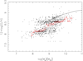
The differences between the $T_{\rm e}$ method and $R_{23}$ method are quite clear, as shown in Figure 7. For a significant part of the galaxies, the $R_{23}$ method gives much higher oxygen abundances than the $T_{\rm e}$ method. It seems that the $T_{\rm e}$-based oxygen abundances have an upper limit of $12+\log{\rm(O/H)}$ around 8.5. Above this metallicity, it is very difficult to excite the collision excitation line [O iii]$\lambda$4363 in the ionized nebulae, thus it becomes very difficult to obtain their electron temperature and the direct oxygen abundances. More physical scenarios can be found in Section 4.1. It also seems the sample galaxies are divided into two populations following $12+\log{\rm(O/H)}_{R_{23}}$. [Yin et al.(2007)Yin, Liang, Hammer et al.] have explained the reason in their section 4.1, which could possibly be related to how secondary nitrogen enrichment is treated in the [Charlot & Longhetti(2001)] models which MPA/JHU used to derive the metallicities of the galaxies. The discrepancy between the oxygen abundances from the $R_{23}$ and $T_{\rm e}$ methods is more obvious with increasing stellar masses in the galaxies.

The differences between abundances from the $R_{23}$ and $T_{\rm e}$ methods are larger following the increasing stellar masses although the scatters are obvious. This could be due to the bias of the sample themselves, i.e. lower metallicity ones were selected relative to the cases of more massive galaxies; Or perhaps this discrepancy is consistent with the suggestion in the abstract of Stasinska (2005): We find that, for metallicities larger than solar, the computed abundances deviate systematically from the real ones, generally by larger amounts for more metal-rich H ii regions.

4 Deriving the mass-metallicity relations of galaxies from $T_{\rm e}$-based oxygen abundances

4.1 Can the [O iii]$\lambda$4363 Selected Galaxies be Good Representatives of the Whole Population of Galaxies?

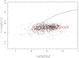
When we try to derive the relations of stellar masses and metallicities of galaxies, we would like to take the galaxies having $T_{\rm e}$ estimates and $T_{\rm e}$-based O/H. However, the question is: Can the galaxies selected with [O iii]$\lambda$4363 be good representatives of the whole population of galaxies? To understand this, we put all our sample galaxies in the MZR and compare with the main sample of SDSS galaxies. These are given in Figure 8. Both the abundances from the $T_{\rm e}$-method (the left panel) and strong-line method (the right panel) are compared with Tremonti’s results (the solid line) from the SDSS main galaxy sample in terms of MZR. In both panels, the discrepancies between the data points and the solid line are quite clear, meaning these objects could not be ideal representatives of the general population of galaxies. They could be biased to galaxies with lower metallicity. Comparing the left to the right panels, it is clear that an obvious difference exists between the $T_{\rm e}$-based cases and the oxygen abundances derived with the strong line method. The dashed and dot-dashed lines show their median trends, respectively.

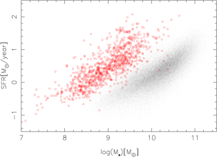
To understand the real reason for such a discrepancy and to check how probable it is that galaxies with detected [O iii]$\lambda$4363 represent the properties of a general population of galaxies, we plot the relations of SFR vs. stellar mass for galaxies in our sample and the ones in the SDSS main galaxy sample. This is given in Figure 9. The discrepancy is quite clear. The galaxies in our sample are more biased to the ones having higher SFRs than the normal galaxies at a given stellar mass. This can be understood since these low-metallicity galaxies should have strong emission lines and higher SFRs.

Therefore, we should be very careful if we want to use the galaxies having $T_{\rm e}$([O iii]) estimates and $T_{\rm e}$-based oxygen abundances to derive the MZR of galaxies, since maybe they are not the typical representatives of the general population of galaxies.

Here we may agree with [Stasińska(2005)]: for the metal-rich (massive) ones, using [O iii]$\lambda$4363 leads to a strong selection bias towards galaxies with low metal abundance.

Shown in Figures 8 and 9, the selected galaxies with reliable [O iii]$\lambda$4363 measurements are biased to low metallicities. This can be understood from the basic physics of photoionized nebulae (Garnett 1992; Stasinska 2002; Ferland 2003). [O iii] is usually the most efficient coolant in ionized nebulae. In the HII region of metal-poor galaxies, there are few cooling ions in the interstellar medium; because the temperature of plasma is high, more $\rm O^{++}$ ions stay in higher energy states, so the [O iii]$\lambda$4363 is easily measured. At high metallicity, cooling is efficient since the heavy elements enforce the cooling effect; the temperature is low, the collision excitation to higher energy states is greatly reduced, and therefore the temperature-sensitive emission lines are very difficult to detect. The emission lines with lower excitation potential could be detected more easily, such as the strong emission lines of [O iii]$\lambda\lambda$4959,5007.

Figure 8: The 12 + log(O/H) versus $\log(M_{*})$ relationship. The corresponding stellar masses are the median values from SDSS. The dots show 947 star-forming galaxies from our work. The triangles show the median from the data in each bin. The dashed and dot-dashed lines show the fitted results with the median data, respectively. Left: oxygen abundances are calculated with the $T_{\rm e}$ method; Right: oxygen abundances are calculated with the $R_{23}$ method.

Figure 9: The relations of SFR vs. stellar mass. The circles are the galaxies whose [O iii]$\lambda$4363 is larger than 5$\sigma$. The small dots are those from the SDSS main galaxy sample.

4.2 Re-deriving the Mass-metallicity Relations with a Wide Range of Stellar Mass from $10^{6}~{}M_{\odot}$ to $10^{11}~{}M_{\odot}$

Figure 10: Fit of the mass-metallicity relations with [Lee et al.(2006)Lee, Skillman, Cannon et al.] and [Liang et al.(2007)Liang, Hammer, Yin et al.] data in a wide range of stellar mass from 10${}^{6}~{}M_{\odot}$ to 10${}^{11}~{}M_{\odot}$. The data follow a straight line well (the black solid line). This shows the MZRs of galaxies whose oxygen abundance is derived from the $T_{\rm e}$ method. The dotted line shows the one from the [Liang et al.(2007)Liang, Hammer, Yin et al.] data. [Lee et al.(2006)Lee, Skillman, Cannon et al.] fit the data to a line which is shown as the dashed line. The fit from [Tremonti et al.(2004)Tremonti, Heckman, Kauffmann et al.] is the dot-dot-dashed line, and the dot-dashed line shows the fit for our sample of galaxies discussed in Sects. 2 and 3.

Figure 11: Combining the data from [Lee et al.(2006)Lee, Skillman, Cannon et al.], [Liang et al.(2007)Liang, Hammer, Yin et al.] and [Andrews & Martini(2013)] altogether, we get their fitted line which is shown as a thick solid line. We do a linear fit with data from [Lee et al.(2006)Lee, Skillman, Cannon et al.] and [Andrews & Martini(2013)], shown as a thin solid line. We also fit data from [Lee et al.(2006)Lee, Skillman, Cannon et al.] and [Andrews & Martini(2013)] with a polynomial which is plotted as a dashed line. We display the fitted line of data from [Lee et al.(2006)Lee, Skillman, Cannon et al.] and [Liang et al.(2007)Liang, Hammer, Yin et al.] with a dotted line. The fits from [Tremonti et al.(2004)Tremonti, Heckman, Kauffmann et al.] and from our sample of galaxies are also shown as the dot-dot-dashed line and the dot-dashed line, respectively.

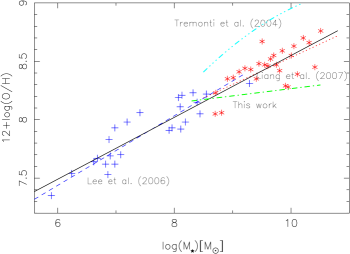
It is necessary to re-derive the relationship between (O/H) abundances and stellar masses for a wide range of stellar mass. Here we take the sample of galaxies from [Lee et al.(2006)Lee, Skillman, Cannon et al.] for low mass galaxies down to 10${}^{11}\,M_{\odot}$, and [Liang et al.(2007)Liang, Hammer, Yin et al.] and [Andrews & Martini(2013)] for massive galaxies obtained through stacking the spectra of the multiple galaxies. [Liang et al.(2007)Liang, Hammer, Yin et al.] measured $T_{\rm e}$[O ii] from the [O ii]$\lambda\lambda$ 7320, 7330 lines and then inferred $T_{\rm e}$[O iii] (and the $\rm O^{++}$ ionic abundance) from analyzing the $t_{2}-t_{3}$ relation shown in our Equation (3). [Andrews & Martini(2013)] measured both $T_{\rm e}$[O iii] and $T_{\rm e}$[O ii] for some stacked objects. These differences could be partly responsible for the offset between [Andrews & Martini(2013)] and [Liang et al.(2007)Liang, Hammer, Yin et al.] in MZR.

By combining data from [Lee et al.(2006)Lee, Skillman, Cannon et al.] and those from [Liang et al.(2007)Liang, Hammer, Yin et al.] or [Andrews & Martini(2013)], we can derive the MZR of galaxies with $T_{\rm e}$-based O/H abundances for a wide range of stellar masses from 10⁶ to 10${}^{11}M_{\odot}$.

The relations derived from the joint sample of [Lee et al.(2006)Lee, Skillman, Cannon et al.] and [Liang et al.(2007)Liang, Hammer, Yin et al.] are shown in Figure 11. [Liang et al.(2007)Liang, Hammer, Yin et al.] gave an equation $12+\log({\rm O/H})=6.223+0.231\times\log M_{*}$ (the dotted line in Fig. 11) and [Lee et al.(2006)Lee, Skillman, Cannon et al.] present the equation $12+\log({\rm O/H})=5.65+0.298\times\log M_{*}$ (the dashed line) for their respective samples. The new relation of MZR covering a wide range of stellar mass is given as (the solid line in Fig. 11)

$$12+\log({\rm O/H})=0.260\log M_{*}+5.950\,.$$ (9)

In Figure 11, the median trend of the objects detected with [O iii]$\lambda$4363, our working sample, is shown as the dot-dashed line, and the trend of [Tremonti et al.(2004)Tremonti, Heckman, Kauffmann et al.] for the SDSS main galaxy sample is shown as the dot-dot-dashed line.

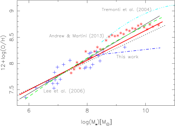
We also derive the MZR from the joint sample of [Lee et al.(2006)Lee, Skillman, Cannon et al.] and [Andrews & Martini(2013)] in this wide range of stellar mass. We fit these data with a least squares linear fit. The result is shown by the thin solid line in Figure 11. The fitting result is as follows

$$12+\log({\rm O/H})=0.329\log M_{*}+5.453\,.$$ (10)

We also fit data from [Lee et al.(2006)Lee, Skillman, Cannon et al.] and [Andrews & Martini(2013)] with a polynomial shown as the dashed line in Figure 11. The fitted polynomial is as follows (the dashed line)

$$12+\log({\rm O/H})=-0.01417(\log M_{*})^{2}+0.56430\log M_{*}+4.49612\,{.}$$ (11)

The dotted line in Figure 11 is from Equation (9), which is the solid one in Figure 11. The difference between [Liang et al.(2007)Liang, Hammer, Yin et al.] and [Andrews & Martini(2013)] in the metal-rich region is more obvious. This could be due to several reasons, such as [Liang et al.(2007)Liang, Hammer, Yin et al.] use a smaller sample, i.e. only selecting those objects having higher equivalent width ([O ii]), which could be slightly biased to lower metallicity, and the method in [Andrews & Martini(2013)] (IRAF) overestimates the log($\rm O^{++}/\rm H^{+}$) by 0.1 dex compared with the method used in [Liang et al.(2007)Liang, Hammer, Yin et al.] (Izotov 2006 formula) (see the left panel of Fig. 4).

To minimize the bias from different samples in different studies, we combine the data from [Lee et al.(2006)Lee, Skillman, Cannon et al.], [Liang et al.(2007)Liang, Hammer, Yin et al.] and [Andrews & Martini(2013)] altogether and get the least squares fit for their mass-metallicity relations. The fitted line is shown as a thick solid line in Figure 11. For comparison, we display the fitted line from the [Lee et al.(2006)Lee, Skillman, Cannon et al.] and [Liang et al.(2007)Liang, Hammer, Yin et al.] data with the dotted line and the line from [Lee et al.(2006)Lee, Skillman, Cannon et al.] and [Andrews & Martini(2013)] data with the thin solid line. The MZR fitted with the three data sets is given as

$$12+\log({\rm O/H})=0.283\log M_{*}+5.798\,.$$ (12)

5 summary

We select 947 star-forming galaxies from SDSS, which have detected [O iii]$\lambda$4363 emission lines. This can help to reliably estimate their electron temperature $T_{\rm e}$ and then $T_{\rm e}$-based oxygen abundances. With this sample, we first carefully compare the electron temperature in high ionization regions, $t_{3}$, from different methods and that in low ionization regions, $t_{2}$, from different methods. Then the resulting ionic abundances $\rm O^{++}$/H⁺ and $\rm O^{+}$/$\rm H^{+}$ are compared correspondingly. In the second part of this work, we derive the MZR from the $T_{\rm e}$-based oxygen abundances of galaxies from literature in a wide range of stellar mass, from 10${}^{6}~{}M_{\odot}$ to 10${}^{11}~{}M_{\odot}$. We find that

• The $t_{3}$ electron temperatures derived from [Izotov et al.(2006)Izotov, Stasińska, Meynet, Guseva, & Thuan] and temden.nebular in stadas.iraf are quite similar.

• The $t_{2}$ electron temperatures resulting from relations of three analyses that considered $t_{2}$–$t_{3}$ show obvious differences, which result in slightly different oxygen abundances.

• The ionic abundances $\rm O^{++}/\rm H^{+}$ are higher than $\rm O^{+}/\rm H^{+}$ for most cases.

• The $T_{\rm e}$-derived and the strong-line derived oxygen abundances show a clear discrepancy, which is more obvious with increasing stellar mass $\log(M_{*})$.

• The sample of galaxies from SDSS with detected [O iii]$\lambda$4363 have lower metallicities and higher SFRs. They may not be representative of the whole population of galaxies and their properties.

• We gather the galaxies having $T_{\rm e}$ and $T_{\rm e}$-derived oxygen abundances in a wide range of stellar mass from 10${}^{6}~{}M_{\odot}$ to 10${}^{11}~{}M_{\odot}$ (Lee et al. (2006) for low mass galaxies, and [Liang et al.(2007)Liang, Hammer, Yin et al.] and [Andrews & Martini(2013)] for massive galaxies). Then we derive new relations of stellar masses and metallicities by combining the data from low mass to massive ones.

In the future, more data should be obtained, especially in the metal-poor region; more work should be done to analyze the mass-metallicity relation in detail based on the $T_{\rm e}$-derived oxygen abundances.