Multipair Full-Duplex Relaying with Massive Arrays and Linear Processing

Abstract

We consider a multipair decode-and-forward relay channel, where multiple sources transmit simultaneously their signals to multiple destinations with the help of a full-duplex relay station. We assume that the relay station is equipped with massive arrays, while all sources and destinations have a single antenna. The relay station uses channel estimates obtained from received pilots and zero-forcing (ZF) or maximum-ratio combining/maximum-ratio transmission (MRC/MRT) to process the signals. To reduce significantly the loop interference effect, we propose two techniques: i) using a massive receive antenna array; or ii) using a massive transmit antenna array together with very low transmit power at the relay station. We derive an exact achievable rate in closed-form for MRC/MRT processing and an analytical approximation of the achievable rate for ZF processing. This approximation is very tight, especially for large number of relay station antennas. These closed-form expressions enable us to determine the regions where the full-duplex mode outperforms the half-duplex mode, as well as, to design an optimal power allocation scheme. This optimal power allocation scheme aims to maximize the energy efficiency for a given sum spectral efficiency and under peak power constraints at the relay station and sources. Numerical results verify the effectiveness of the optimal power allocation scheme. Furthermore, we show that, by doubling the number of transmit/receive antennas at the relay station, the transmit power of each source and of the relay station can be reduced by $1.5$dB if the pilot power is equal to the signal power, and by $3$dB if the pilot power is kept fixed, while maintaining a given quality-of-service.

I Introduction

Multiple-input multiple-output (MIMO) systems that use antenna arrays with a few hundred antennas for multiuser operation (popularly called “Massive MIMO”) is an emerging technology that can deliver all the attractive benefits of traditional MIMO, but at a much larger scale [2, 3, 4]. Such systems can reduce substantially the effects of noise, fast fading and interference and provide increased throughput. Importantly, these attractive features of massive MIMO can be reaped using simple signal processing techniques and at a reduction of the total transmit power. As a result, not surprisingly, massive MIMO combined with cooperative relaying is a strong candidate for the development of future energy-efficient cellular networks [4, 5].

On a parallel avenue, full-duplex relaying has received a lot of research interest, for its ability to recover the bandwidth loss induced by conventional half-duplex relaying. With full-duplex relaying, the relay node receives and transmits simultaneously on the same channel [6, 7]. As such, full-duplex utilizes the spectrum resources more efficiently. Over the recent years, rapid progress has been made on both theory and experimental hardware platforms to make full-duplex wireless communication an efficient practical solution [8, 9, 10, 11, 12, 13]. The benefit of improved spectral efficiency in the full-duplex mode comes at the price of loop interference due to signal leakage from the relay’s output to the input [9, 10]. A large amplitude difference between the loop interference and the received signal coming from the source can exceed the dynamic range of the analog-to-digital converter at the receiver side, and, thus, its mitigation is crucial for full-duplex operation [13, 14]. Note that how to overcome the detrimental effects of loop interference is a highly active area in full-duplex research.

Traditionally, loop interference suppression is performed in the antenna domain using a variety of passive techniques that electromagnetically shield the transmit antenna from the receive antenna. As an example, directional antennas can be used to place a null at the receive antenna. Since the distance between the transmit and receive arrays is short, such techniques require significant levels of loop interference mitigation and, hence, are hard to realize. On the other hand, active time domain loop interference cancellation techniques use the knowledge of the interfering signal to pre-cancel the loop interference in the radio frequency signal and achieve higher levels of loop interference suppression. However, they demand advanced noise cancellation methods and sophisticated electronic implementation [8]. Yet, MIMO processing provides an effective means of suppressing the loop interference in the spatial domain. With multiple transmit or receive antennas at the full-duplex relay, precoding solutions, such as zero-forcing (ZF), can be deployed to mitigate the loop interference effects. Although sub-optimal in general, simple ZF-based precoder can completely cancel the loop interference and remove the closed-loop between the relay’s input and output. Several papers have considered spatial loop interference suppression; for example, [10] proposes to direct the loop interference of a full-duplex decode-and-forward (DF) relay to the least harmful spatial dimensions. In [8], assuming a multiple antenna relay, a range of spatial suppression techniques including precoding and antenna selection is analyzed. In [15], several antenna sub-set selection schemes are proposed aiming to suppress loop interference at the relay’s transmit side. More recently, [16] analyzed several antenna selection schemes for spatial loop interference suppression in a MIMO relay channel.

Different from the majority of existing works in the literature, which consider systems that deploy only few antennas, in this paper we consider a massive MIMO full-duplex relay architecture. The large number of spatial dimensions available in a massive MIMO system can be effectively used to suppress the loop interference in the spatial domain. We assume that a group of $K$ sources communicate with a group of $K$ destinations using a massive MIMO full-duplex relay station. Specifically, in this multipair massive MIMO relay system, we deploy two processing schemes, namely, ZF and maximum ratio combining (MRC)/maximal ratio transmission (MRT) with full-duplex relay operation. Recall that linear processing techniques, such as ZF or MRC/MRT processing, are low-complexity solutions that are anticipated to be utilized in massive MIMO topologies. Their main advantage is that in the large-antenna limit, they can perform as well as non-linear schemes (e.g., maximum-likelihood) [2, 5, 17]. Our system setup could be applied in cellular networks, where several users transmit simultaneously signals to several other users with the help of a relay station (infrastructure-based relaying). Note that, newly evolving wireless standards, such as LTE-Advanced, promote the use of relays (with unique cell ID and right for radio resource management) to serve as low power base stations [18, 19].

We investigate the achievable rate and power efficiency of the aforementioned full-duplex system setup. Moreover, we compare full-duplex and half-duplex modes and show the benefit of choosing one over the other (depending on the loop interference level of the full-duplex mode). Although the current work uses techniques related to those in Massive MIMO, we investigate a substantially different setup. Specifically, previous works related to Massive MIMO systems [2, 3, 4, 22] considered the uplink or the downlink of multiuser MIMO channels. In contrast, we consider multipair full-duplex relaying channels with massive arrays at the relay station. As a result, our new contributions are very different from the existing works on Massive MIMO. The main contributions of this paper are summarized as follows:

1. We show that the loop interference can be significantly reduced, if the relay station is equipped with a large receive antenna array or/and is equipped with a large transmit antenna array. At the same time, the inter-pair interference and noise effects disappear. Furthermore, when the number of relay station transmit antennas, $N_{\mathrm{tx}}$, and the number of relay station receive antennas, $N_{\mathrm{rx}}$, are large, we can scale down the transmit powers of each source and of the relay proportionally to $1/N_{\mathrm{rx}}$ and $1/N_{\mathrm{tx}}$, respectively, if the pilot power is kept fixed, and proportionally to $1/\sqrt{N_{\mathrm{rx}}}$ and $1/\sqrt{N_{\mathrm{tx}}}$, respectively, if the pilot power and the data power are the same.

2. We derive exact and approximate closed-form expressions for the end-to-end (e2e) achievable rates of MRC/MRT and ZF processing, respectively. These simple closed-form expressions enable us to obtain important insights as well as to compare full-duplex and half-duplex operation and demonstrate which mode yields better performance. As a general remark, the full-duplex mode improves significantly the overall system performance when the loop interference level is low. In addition, we propose the use of a hybrid mode for each large-scale fading realization, which switches between the full-duplex and half-duplex modes, to maximize the sum spectral efficiency.

3. We design an optimal power allocation algorithm for the data transmission phase, which maximizes the energy efficiency for a desired sum spectral efficiency and under peak power constraints at the relay station and sources. This optimization problem can be approximately solved via a sequence of geometric programs (GPs). Our numerical results indicate that the proposed power allocation improves notably the performance compared to uniform power allocation.

Notation: We use boldface upper- and lower-case letters to denote matrices and column vectors, respectively. The superscripts $()^{\ast}$, $()^{T}$, and $()^{H}$ stand for the conjugate, transpose, and conjugate-transpose, respectively. The Euclidean norm, the trace, the expectation, and the variance operators are denoted by $\|\cdot\|$, $\operatorname{\mathrm{tr}}\left(\cdot\right)$, $\mathbb{E}\left\{\cdot\right\}$, and $\operatorname{\mathbb{V}\mathrm{ar}}\left(\cdot\right)$, respectively. The notation $\mathop{\to}\limits^{a.s.}$ means almost sure convergence, while $\mathop{\to}\limits^{d}$ means convergence in distribution. Finally, we use ${\mathbf{z}}\sim\mathcal{CN}\left({\mathbf{0}},{{\mathbf{\Sigma}}}\right)$ to denote a circularly symmetric complex Gaussian vector ${\mathbf{z}}$ with zero mean and covariance matrix ${\mathbf{\Sigma}}$.

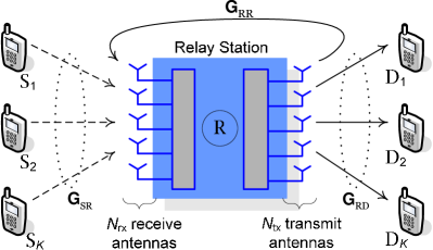
Figure 1: Multipair full-duplex relaying system.

II System Model

Figure 1 shows the considered multipair DF relaying system where $K$ communication pairs $({\tt S}_{k},{\tt D_{k}})$, $k=1,\ldots,K$, share the same time-frequency resource and a common relay station, ${\tt R}$. The $k$th source, ${\tt S}_{k}$, communicates with the $k$th destination, ${\tt D}_{k}$, via the relay station, which operates in a full-duplex mode. All source and destination nodes are equipped with a single antenna, while the relay station is equipped with $N_{\mathrm{rx}}$ receive antennas and $N_{\mathrm{tx}}$ transmit antennas. The total number of antennas at the relay station is $N=N_{\mathrm{rx}}+N_{\mathrm{tx}}$. We assume that the hardware chain calibration is perfect so that the channel from the relay station to the destination is reciprocal [4]. Further, the direct links among ${\tt S}_{k}$ and ${\tt D_{k}}$ do not exist due to large path loss and heavy shadowing. Our network configuration is of practical interest, for example, in a cellular setup, where inter-user communication is realized with the help of a base station equipped with massive arrays.

At time instant $i$, all $K$ sources ${\tt S}_{k}$, $k=1,...,K$, transmit simultaneously their signals, $\sqrt{p_{\tt{S}}}x_{k}\left[i\right]$, to the relay station, while the relay station broadcasts $\sqrt{p_{\tt{R}}}{\mathbf{s}}\left[i\right]\in\mathbb{C}^{N_{\mathrm{tx}}\times 1}$ to all $K$ destinations. Here, we assume that $\operatorname{\mathtt{E}}\left\{\left|x_{k}\left[i\right]\right|^{2}\right\}=1$ and $\operatorname{\mathtt{E}}\left\{\left\|{\mathbf{s}}\left[i\right]\right\|^{2}\right\}=1$ so that $p_{\tt{S}}$ and $p_{\tt{R}}$ are the average transmit powers of each source and of the relay station. Since the relay station receives and transmits at the same frequency, the received signal at the relay station is interfered by its own transmitted signal, ${\mathbf{s}}\left[i\right]$. This is called loop interference. Denote by ${\mathbf{x}}\left[i\right]\triangleq\left[x_{1}\left[i\right]~{}x_{2}\left[i\right]~{}...~{}x_{K}\left[i\right]\right]^{T}$. The received signals at the relay station and the $K$ destinations are given by [8]

$${\mathbf{y}}_{\tt R}\left[i\right] =\sqrt{p_{\tt{S}}}{\mathbf{G}}_{\tt SR}{\mathbf{x}}\left[i\right]+\sqrt{p_{\tt{R}}}{\mathbf{G}}_{\tt RR}{\mathbf{s}}\left[i\right]+{\mathbf{n}}_{\tt R}\left[i\right],$$ (1)

$${\mathbf{y}}_{\tt{D}}\left[i\right] =\sqrt{p_{\tt{R}}}{\mathbf{G}}_{\tt RD}^{T}{\mathbf{s}}\left[i\right]+{\mathbf{n}}_{\tt D}\left[i\right],$$ (2)

respectively, where ${\mathbf{G}}_{\tt SR}\in\mathbb{C}^{N_{\mathrm{rx}}\times K}$ and ${\mathbf{G}}_{\tt RD}^{T}\in\mathbb{C}^{K\times N_{\mathrm{tx}}}$ are the channel matrices from the $K$ sources to the relay station’s receive antenna array and from the relay station’s transmit antenna array to the $K$ destinations, respectively. The channel matrices account for both small-scale fading and large-scale fading. More precisely, ${\mathbf{G}}_{\tt SR}$ and ${\mathbf{G}}_{\tt RD}$ can be expressed as ${\mathbf{G}}_{\tt SR}={\mathbf{H}}_{\tt SR}{\mathbf{D}}_{\tt SR}^{1/2}$ and ${\mathbf{G}}_{\tt RD}={\mathbf{H}}_{\tt RD}{\mathbf{D}}_{\tt RD}^{1/2}$, where the small-scale fading matrices ${\mathbf{H}}_{\tt SR}$ and ${\mathbf{H}}_{\tt RD}$ have independent and identically distributed (i.i.d.) $\mathcal{CN}\left({0},{1}\right)$ elements, while ${\mathbf{D}}_{\tt SR}$ and ${\mathbf{D}}_{\tt RD}$ are the large-scale fading diagonal matrices whose $k$th diagonal elements are denoted by $\beta_{{\tt SR},k}$ and $\beta_{{\tt RD},k}$, respectively. The above channel models rely on the favorable propagation assumption, which assumes that the channels from the relay station to different sources and destinations are independent [4]. The validity of this assumption was demonstrated in practice, even for massive arrays [20]. Also in (1), ${\mathbf{G}}_{\tt RR}\in\mathbb{C}^{N_{\mathrm{rx}}\times N_{\mathrm{tx}}}$ is the channel matrix between the transmit and receive arrays which represents the loop interference. We model the loop interference channel via the Rayleigh fading distribution, under the assumptions that any line-of-sight component is efficiently reduced by antenna isolation and the major effect comes from scattering. Note that if hardware loop interference cancellation is applied, ${\mathbf{G}}_{\tt RR}$ represents the residual interference due to imperfect loop interference cancellation. The residual interfering link is also modeled as a Rayleigh fading channel, which is a common assumption made in the existing literature [8]. Therefore, the elements of ${\mathbf{G}}_{\tt RR}$ can be modeled as i.i.d. $\mathcal{CN}\left({0},{\sigma_{\tt LI}^{2}}\right)$ random variables, where $\sigma_{\tt LI}^{2}$ can be understood as the level of loop interference, which depends on the distance between the transmit and receive antenna arrays or/and the capability of the hardware loop interference cancellation technique [9]. Here, we assume that the distance between the transmit array and the receive array is much larger than the inter-element distance, such that the channels between the transmit and receive antennas are i.i.d.; also, ${\mathbf{n}}_{\tt R}\left[i\right]$ and ${\mathbf{n}}_{\tt D}\left[i\right]$ are additive white Gaussian noise (AWGN) vectors at the relay station and the $K$ destinations, respectively. The elements of ${\mathbf{n}}_{\tt R}\left[i\right]$ and ${\mathbf{n}}_{\tt D}\left[i\right]$ are assumed to be i.i.d. $\mathcal{CN}\left({0},{1}\right)$.

II-A Channel Estimation

In practice, the channels ${{\mathbf{G}}}_{\tt SR}$ and ${{\mathbf{G}}}_{\tt RD}$ have to be estimated at the relay station. The standard way of doing this is to utilize pilots [2]. To this end, a part of the coherence interval is used for channel estimation. All sources and destinations transmit simultaneously their pilot sequences of $\tau$ symbols to the relay station. The received pilot matrices at the relay receive and transmit antenna arrays are given by

$${\mathbf{Y}}_{\mathrm{rp}} =\sqrt{\tau p_{\mathrm{p}}}{\mathbf{G}}_{\tt SR}{\mathbf{\Phi}}_{\tt S}+\sqrt{\tau p_{\mathrm{p}}}\bar{{\mathbf{G}}}_{\tt RD}{\mathbf{\Phi}}_{\tt D}+{\mathbf{N}}_{\mathrm{rp}},$$ (3)

$${\mathbf{Y}}_{\mathrm{tp}} =\sqrt{\tau p_{\mathrm{p}}}\bar{{\mathbf{G}}}_{\tt SR}{\mathbf{\Phi}}_{\tt S}+\sqrt{\tau p_{\mathrm{p}}}{\mathbf{G}}_{\tt RD}{\mathbf{\Phi}}_{\tt D}+{\mathbf{N}}_{\mathrm{tp}},$$ (4)

respectively, where $\bar{{\mathbf{G}}}_{\tt SR}\in\mathbb{C}^{N_{\mathrm{tx}}\times K}$ and $\bar{{\mathbf{G}}}_{\tt RD}\in\mathbb{C}^{N_{\mathrm{rx}}\times K}$ are the channel matrices from the $K$ sources to the relay station’s transmit antenna array and from the $K$ destinations to the relay station’s receive antenna array, respectively; $p_{\mathrm{p}}$ is the transmit power of each pilot symbol, ${\mathbf{N}}_{\mathrm{rp}}$ and ${\mathbf{N}}_{\mathrm{tp}}$ are AWGN matrices which include i.i.d. $\mathcal{CN}\left({0},{1}\right)$ elements, while the $k$th rows of ${\mathbf{\Phi}}_{\tt S}\in\mathbb{C}^{K\times\tau}$ and ${\mathbf{\Phi}}_{\tt D}\in\mathbb{C}^{K\times\tau}$ are the pilot sequences transmitted from ${\tt S}_{k}$ and ${\tt D}_{k}$, respectively. All pilot sequences are assumed to be pairwisely orthogonal, i.e., ${\mathbf{\Phi}}_{\tt S}{\mathbf{\Phi}}_{\tt S}^{H}={\mathbf{I}}_{K}$, ${\mathbf{\Phi}}_{\tt D}{\mathbf{\Phi}}_{\tt D}^{H}={\mathbf{I}}_{K}$, and ${\mathbf{\Phi}}_{\tt S}{\mathbf{\Phi}}_{\tt D}^{H}={\mathbf{0}}_{K}$. This requires that $\tau\geq 2K$.

We assume that the relay station uses minimum mean-square-error (MMSE) estimation to estimate ${\mathbf{G}}_{\tt SR}$ and ${\mathbf{G}}_{\tt RD}$. The MMSE channel estimates of ${\mathbf{G}}_{\tt SR}$ and ${\mathbf{G}}_{\tt RD}$ are given by [21]

$$\hat{{\mathbf{G}}}_{\tt SR}=\frac{1}{\sqrt{\tau p_{\mathrm{p}}}}{\mathbf{Y}}_{\mathrm{rp}}{\mathbf{\Phi}}_{\tt S}^{H}\tilde{{\mathbf{D}}}_{\tt SR}={\mathbf{G}}_{\tt SR}\tilde{{\mathbf{D}}}_{\tt SR}+\frac{1}{\sqrt{\tau p_{\mathrm{p}}}}{\mathbf{N}}_{\tt S}\tilde{{\mathbf{D}}}_{\tt SR},$$ (5)

$$\hat{{\mathbf{G}}}_{\tt RD}=\frac{1}{\sqrt{\tau p_{\mathrm{p}}}}{\mathbf{Y}}_{\mathrm{tp}}{\mathbf{\Phi}}_{\tt D}^{H}\tilde{{\mathbf{D}}}_{\tt RD}={\mathbf{G}}_{\tt RD}\tilde{{\mathbf{D}}}_{\tt RD}+\frac{1}{\sqrt{\tau p_{\mathrm{p}}}}{\mathbf{N}}_{\tt D}\tilde{{\mathbf{D}}}_{\tt RD},$$ (6)

respectively, where $\tilde{{\mathbf{D}}}_{\tt SR}\triangleq\left(\frac{{{\mathbf{D}}}_{\tt SR}^{-1}}{\tau p_{\mathrm{p}}}+{\mathbf{I}}_{K}\right)^{-1}$, $\tilde{{\mathbf{D}}}_{\tt RD}\triangleq\left(\frac{{{\mathbf{D}}}_{\tt RD}^{-1}}{\tau p_{\mathrm{p}}}+{\mathbf{I}}_{K}\right)^{-1}$, ${\mathbf{N}}_{\tt S}\triangleq{\mathbf{N}}_{\mathrm{rp}}{\mathbf{\Phi}}_{\tt S}^{H}$ and ${\mathbf{N}}_{\tt D}\triangleq{\mathbf{N}}_{\mathrm{tp}}{\mathbf{\Phi}}_{\tt D}^{H}$. Since the rows of ${\mathbf{\Phi}}_{\tt S}$ and ${\mathbf{\Phi}}_{\tt D}$ are pairwisely orthogonal, the elements of ${\mathbf{N}}_{\tt S}$ and ${\mathbf{N}}_{\tt D}$ are i.i.d. $\mathcal{CN}\left({0},{1}\right)$ random variables. Let $\boldsymbol{\mathcal{E}}_{\tt SR}$ and $\boldsymbol{\mathcal{E}}_{\tt RD}$ be the estimation error matrices of ${\mathbf{G}}_{\tt SR}$ and ${\mathbf{G}}_{\tt RD}$, respectively. Then,

$${\mathbf{G}}_{\tt SR} =\hat{{\mathbf{G}}}_{\tt SR}+\boldsymbol{\mathcal{E}}_{\tt SR},$$ (7)

$${\mathbf{G}}_{\tt RD} =\hat{{\mathbf{G}}}_{\tt RD}+\boldsymbol{\mathcal{E}}_{\tt RD}.$$ (8)

From the property of MMSE channel estimation, $\hat{{\mathbf{G}}}_{\tt SR}$, $\boldsymbol{\mathcal{E}}_{\tt SR}$, $\hat{{\mathbf{G}}}_{\tt RD}$, and $\boldsymbol{\mathcal{E}}_{\tt RD}$ are independent [21]. Furthermore, we have that the rows of $\hat{{\mathbf{G}}}_{\tt SR}$, $\boldsymbol{\mathcal{E}}_{\tt SR}$, $\hat{{\mathbf{G}}}_{\tt RD}$, and $\boldsymbol{\mathcal{E}}_{\tt RD}$ are mutually independent and distributed as $\mathcal{CN}\left({{\mathbf{0}}},{\hat{{\mathbf{D}}}_{{\tt SR}}}\right)$, $\mathcal{CN}\left({{\mathbf{0}}},{{{\mathbf{D}}}_{{\tt SR}}-\hat{{\mathbf{D}}}_{{\tt SR}}}\right)$, $\mathcal{CN}\left({{\mathbf{0}}},{\hat{{\mathbf{D}}}_{{\tt RD}}}\right)$, and $\mathcal{CN}\left({{\mathbf{0}}},{{{\mathbf{D}}}_{{\tt RD}}-\hat{{\mathbf{D}}}_{{\tt RD}}}\right)$, respectively, where $\hat{{\mathbf{D}}}_{{\tt SR}}$ and $\hat{{\mathbf{D}}}_{{\tt RD}}$ are diagonal matrices whose $k$th diagonal elements are $\sigma_{{\tt SR},k}^{2}\triangleq\frac{\tau p_{\mathrm{p}}\beta_{{\tt SR},k}^{2}}{\tau p_{\mathrm{p}}\beta_{{\tt SR},k}+1}$ and $\sigma_{{\tt RD},k}^{2}\triangleq\frac{\tau p_{\mathrm{p}}\beta_{{\tt RD},k}^{2}}{\tau p_{\mathrm{p}}\beta_{{\tt RD},k}+1}$, respectively.

II-B Data Transmission

The relay station considers the channel estimates as the true channels and employs linear processing. More precisely, the relay station uses a linear receiver to decode the signals transmitted from the $K$ sources. Simultaneously, it uses a linear precoding scheme to forward the signals to the $K$ destinations.

II-B1 Linear Receiver

With the linear receiver, the received signal ${\mathbf{y}}_{\tt R}\left[i\right]$ is separated into $K$ streams by multiplying it with a linear receiver matrix ${\mathbf{W}}^{T}$ (which is a function of the channel estimates) as follows:

$${\mathbf{r}}\left[i\right] ={\mathbf{W}}^{T}{\mathbf{y}}_{\tt R}\left[i\right]=\sqrt{p_{\tt{S}}}{\mathbf{W}}^{T}{\mathbf{G}}_{\tt SR}{\mathbf{x}}\left[i\right]+\sqrt{p_{\tt{R}}}{\mathbf{W}}^{T}{\mathbf{G}}_{\tt RR}{\mathbf{s}}\left[i\right]+{\mathbf{W}}^{T}{\mathbf{n}}_{\tt R}\left[i\right].$$ (9)

Then, the $k$th stream ($k$th element of ${\mathbf{r}}\left[i\right]$) is used to decode the signal transmitted from ${\tt S}_{k}$. The $k$th element of ${\mathbf{r}}\left[i\right]$ can be expressed as

$${r}_{k}\left[i\right] =\underbrace{\sqrt{p_{\tt{S}}}{\mathbf{w}}_{k}^{T}{\mathbf{g}}_{{\tt SR},k}{x}_{k}\left[i\right]}_{\text{desired signal}}+\underbrace{\sqrt{p_{\tt{S}}}\sum_{j\neq k}^{K}{\mathbf{w}}_{k}^{T}{\mathbf{g}}_{{\tt SR},j}{x}_{j}\left[i\right]}_{\text{interpair interference}}$$

$$+\underbrace{\sqrt{p_{\tt{R}}}{\mathbf{w}}_{k}^{T}{\mathbf{G}}_{\tt RR}{\mathbf{s}}\left[i\right]}_{\text{loop interference}}+\underbrace{{\mathbf{w}}_{k}^{T}{\mathbf{n}}_{\tt R}\left[i\right]}_{\text{noise}},$$ (10)

where ${\mathbf{g}}_{{\tt SR},k}$, ${\mathbf{w}}_{k}$ are the $k$th columns of ${\mathbf{G}}_{\tt SR}$, ${\mathbf{W}}$, respectively, and ${x}_{k}\left[i\right]$ is the $k$th element of ${\mathbf{x}}\left[i\right]$.

II-B2 Linear Precoding

After detecting the signals transmitted from the $K$ sources, the relay station uses linear precoding to process these signals before broadcasting them to all $K$ destinations. Owing to the processing delay [8], the transmit vector ${\mathbf{s}}\left[i\right]$ is a precoded version of ${\mathbf{x}}\left[i-d\right]$, where $d$ is the processing delay. More precisely,

$${\mathbf{s}}\left[i\right] ={\mathbf{A}}{\mathbf{x}}\left[i-d\right],$$ (11)

where ${\mathbf{A}}\in\mathbb{C}^{N_{\mathrm{tx}}\times K}$ is a linear precoding matrix which is a function of the channel estimates. We assume that the processing delay $d\geq 1$ which guarantees that the receive and transmit signals at the relay station, for a given time instant, are uncorrelated. This is a common assumption for full-duplex systems in the existing literature [9, 11].

From (2) and (11), the received signal at ${\tt D}_{k}$ can be expressed as

$${y}_{{\tt D},k}\left[i\right] =\sqrt{p_{\tt{R}}}{\mathbf{g}}_{{\tt RD},k}^{T}{\mathbf{a}}_{k}{x}_{k}\left[i-d\right]$$

$$+\sqrt{p_{\tt{R}}}\sum_{j\neq k}^{K}{\mathbf{g}}_{{\tt RD},k}^{T}{\mathbf{a}}_{j}{x}_{j}\left[i-d\right]+{n}_{{\tt D},k}\left[i\right],$$ (12)

where ${\mathbf{g}}_{{\tt RD},k}$, ${\mathbf{a}}_{k}$ are the $k$th columns of ${\mathbf{G}}_{\tt RD}$, ${\mathbf{A}}$, respectively, and ${n}_{{\tt D},k}\left[i\right]$ is the $k$th element of ${\mathbf{n}}_{{\tt D}}\left[i\right]$.

II-C ZF and MRC/MRT Processing

In this work, we consider two common linear processing techniques: ZF and MRC/MRT processing.

II-C1 ZF Processing

In this case, the relay station uses the ZF receiver and ZF precoding to process the signals. Due to the fact that all communication pairs share the same time-frequency resource, the transmission of a given pair will be impaired by the transmissions of other pairs. This effect is called “interpair interference”. More explicitly, for the transmission from ${\tt S}_{k}$ to the relay station, the interpair interference is represented by the term $\sqrt{p_{\tt{S}}}\sum_{j\neq k}^{K}{\mathbf{w}}_{k}^{T}{\mathbf{g}}_{{\tt SR},j}{x}_{j}\left[i\right]$, while for the transmission from the relay station to ${\tt D}_{k}$, the interpair interference is $\sqrt{p_{\tt{R}}}\sum_{j\neq k}^{K}{\mathbf{g}}_{{\tt RD},k}^{T}{\mathbf{a}}_{j}{x}_{j}\left[i-d\right]$. With ZF processing, interpair interference is nulled out by projecting each stream onto the orthogonal complement of the interpair interference. This can be done if the relay station has perfect channel state information (CSI). However, in practice, the relay station knows only the estimates of CSI. Therefore, interpair interference and loop interference still exist. We assume that $N_{\mathrm{rx}},N_{\mathrm{tx}}>K$.

The ZF receiver and ZF precoding matrices are respectively given by [22, 23]

$${\mathbf{W}}^{T} ={\mathbf{W}}_{\tt ZF}^{T}\triangleq\left(\hat{{\mathbf{G}}}_{\tt SR}^{H}\hat{{\mathbf{G}}}_{\tt SR}\right)^{-1}\hat{{\mathbf{G}}}_{\tt SR}^{H},$$ (13)

$${\mathbf{A}} ={\mathbf{A}}_{\tt ZF}\triangleq\alpha_{\tt ZF}\hat{{\mathbf{G}}}_{\tt RD}^{\ast}\left(\hat{{\mathbf{G}}}_{\tt RD}^{T}\hat{{\mathbf{G}}}_{\tt RD}^{\ast}\right)^{-1}\!\!\!,$$ (14)

where $\alpha_{\tt ZF}$ is a normalization constant, chosen to satisfy a long-term total transmit power constraint at the relay, i.e., $\operatorname{\mathtt{E}}\left\{\left\|{\mathbf{s}}\left[i\right]\right\|^{2}\right\}=1$. Therefore, we have [23]

$$\alpha_{\tt ZF} =\sqrt{\frac{N_{\mathrm{tx}}-K}{\sum_{k=1}^{K}\sigma_{{\tt RD},k}^{-2}}}.$$ (15)

II-C2 MRC/MRT Processing

The ZF processing neglects the effect of noise and, hence, it works poorly when the signal-to-noise ratio (SNR) is low. By contrast, the MRC/MRT processing aims to maximize the received SNR, by neglecting the interpair interference effect. Thus, MRC/MRT processing works well at low SNRs, and works poorly at high SNRs. With MRC/MRT processing, the relay station uses MRC to detect the signals transmitted from the $K$ sources. Then, it uses the MRT technique to transmit signals towards the $K$ destinations. The MRC receiver and MRT precoding matrices are respectively given by [22, 23]

$${\mathbf{W}}^{T} ={\mathbf{W}}_{\tt MRC}^{T}\triangleq\hat{{\mathbf{G}}}_{\tt SR}^{H},$$ (16)

$${\mathbf{A}} ={\mathbf{A}}_{\tt MRT}\triangleq\alpha_{\tt MRT}\hat{{\mathbf{G}}}_{\tt RD}^{\ast},$$ (17)

where the normalization constant $\alpha_{\tt MRT}$ is chosen to satisfy a long-term total transmit power constraint at the relay, i.e., $\operatorname{\mathtt{E}}\left\{\left\|{\mathbf{s}}\left[i\right]\right\|^{2}\right\}=1$, and we have [23]

$$\alpha_{\tt MRT} =\sqrt{\frac{1}{N_{\mathrm{tx}}\sum_{k=1}^{K}\sigma_{{\tt RD},k}^{2}}}.$$ (18)

III Loop Interference Cancellation with Large Antenna Arrays

In this section, we consider the potential of using massive MIMO technology to cancel the loop interference due to the full-duplex operation at the relay station. Some interesting insights are also presented.

III-A Using a Large Receive Antenna Array ($N_{\mathrm{rx}}\to\infty$)

The loop interference can be canceled out by projecting it onto its orthogonal complement. However, this orthogonal projection may harm the desired signal. Yet, when $N_{\mathrm{rx}}$ is large, the subspace spanned by the loop interference is nearly orthogonal to the desired signal’s subspace and, hence, the orthogonal projection scheme will perform very well. The next question is how to project the loop interference component? It is interesting to observe that, when $N_{\mathrm{rx}}$ grows large, the channel vectors of the desired signal and the loop interference become nearly orthogonal. Therefore, the ZF or the MRC receiver can act as an orthogonal projection of the loop interference. As a result, the loop interferenceI can be reduced significantly by using large $N_{\mathrm{rx}}$ together with the ZF or MRC receiver. This observation is summarized in the following proposition.

Proposition 1

Assume that the number of source-destination pairs, $K$, is fixed. For any finite $N_{\mathrm{tx}}$ or for any $N_{\mathrm{tx}}$, such that $N_{\mathrm{rx}}/N_{\mathrm{tx}}$ is fixed, as $N_{\mathrm{rx}}\to\infty$, the received signal at the relay station for decoding the signal transmitted from ${\tt S}_{k}$ is given by

$${r}_{k}\left[i\right] \mathop{\to}\limits^{a.s.}\sqrt{p_{\tt{S}}}{x}_{k}\left[i\right],~{}\text{for ZF},$$ (19)

$$\frac{{r}_{k}\left[i\right]}{N_{\mathrm{rx}}\sigma_{{\tt SR},k}^{2}} \mathop{\to}\limits^{a.s.}\sqrt{p_{\tt{S}}}{x}_{k}\left[i\right],~{}\text{for MRC/MRT}.$$ (20)

Proof:

See Appendix -A. ∎

The aforementioned results imply that, when $N_{\mathrm{rx}}$ grows to infinity, the loop interference can be canceled out. Furthermore, the interpair interference and noise effects also disappear. The received signal at the relay station after using ZF or MRC receivers includes only the desired signal and, hence, the capacity of the communication link ${\tt S}_{k}\to{\tt R}$ grows without bound. As a result, the system performance is limited only by the performance of the communication link ${\tt R}\to{\tt D}_{k}$ which does not depend on the loop interference.

III-B Using a Large Transmit Antenna Array and Low Transmit Power ($p_{\tt{R}}=E_{\mathsf{R}}/N_{\mathrm{tx}}$, where $E_{\mathsf{R}}$ is Fixed, and $N_{\mathrm{tx}}\to\infty$)

The loop interference depends strongly on the transmit power at the relay station, $p_{\tt{R}}$ and, hence, another way to reduce it is to use low transmit power $p_{\tt{R}}$. Unfortunately, this will also reduce the quality of the transmission link ${\tt R}\to{\tt D}_{k}$ and, hence, the e2e system performance will be degraded. However, with a large relay station transmit antenna array, we can reduce the relay transmit power while maintaining a desired quality-of-service (QoS) of the transmission link ${\tt R}\to{\tt D}_{k}$. This is due to the fact that, when the number of transmit antennas, $N_{\mathrm{tx}}$, is large, the relay station can focus its emitted energy into the physical directions wherein the destinations are located. At the same time, the relay station can purposely avoid transmitting into physical directions where the receive antennas are located and, hence, the loop interference can be significantly reduced. Therefore, we propose to use a very large $N_{\mathrm{tx}}$ together with low transmit power at the relay station. With this method, the loop interference in the transmission link ${\tt S}_{k}\to{\tt R}$ becomes negligible, while the quality of the transmission link ${\tt R}\to{\tt D}_{k}$ is still fairly good. As a result, we can obtain a good e2e performance.

Proposition 2

Assume that $K$ is fixed and the transmit power at the relay station is $p_{\tt{R}}=E_{\mathsf{R}}/N_{\mathrm{tx}}$, where $E_{\mathsf{R}}$ is fixed regardless of $N_{\mathrm{tx}}$. For any finite $N_{\mathrm{rx}}$, as $N_{\mathrm{tx}}\to\infty$, the received signals at the relay station and ${\tt D}_{k}$ converge to

$${r}_{k}\left[i\right] \mathop{\to}\limits^{a.s.}\sqrt{p_{\tt{S}}}{\mathbf{w}}_{k}^{T}{\mathbf{g}}_{{\tt SR},k}{x}_{k}\left[i\right]+\sqrt{p_{\tt{S}}}\sum_{j\neq k}^{K}{\mathbf{w}}_{k}^{T}{\mathbf{g}}_{{\tt SR},j}{x}_{j}\left[i\right]$$

$$+{\mathbf{w}}_{k}^{T}{\mathbf{n}}_{\tt R}\left[i\right],~{}\text{for both ZF and MRC/MRT,}$$ (21)

$${y}_{{\tt D},k}\left[i\right] \mathop{\to}\limits^{a.s.}\left\{\begin{array}[]{l}\sqrt{\frac{E_{\mathsf{R}}}{\sum_{j=1}^{K}\sigma_{{\tt RD},j}^{-2}}}{x}_{k}\left[i-d\right]+{n}_{{\tt D},k}\left[i\right],~{}\text{for ZF,}\\ \sqrt{\frac{\sigma_{{\tt RD},k}^{4}E_{\mathsf{R}}}{\sum_{j=1}^{K}\sigma_{{\tt RD},j}^{2}}}{x}_{k}\left[i-d\right]+{n}_{{\tt D},k}\left[i\right],~{}\text{for MRC/MRT,}\\ \end{array}\right.$$ (24)

respectively.

Proof:

With ZF processing, the loop interference is given by

$$\sqrt{p_{\tt{R}}}{\mathbf{W}}^{T}{\mathbf{G}}_{\tt RR}{\mathbf{s}}\left[i\right] =\sqrt{\frac{\left(N_{\mathrm{tx}}-K\right)E_{\mathsf{R}}}{N_{\mathrm{tx}}\sum_{k=1}^{K}\sigma_{{\tt RD},k}^{-2}}}{\mathbf{W}}_{\tt ZF}^{T}\frac{{\mathbf{G}}_{\tt RR}\hat{{\mathbf{G}}}_{\tt RD}^{\ast}}{N_{\mathrm{tx}}}$$

$$\times\left(\frac{\hat{{\mathbf{G}}}_{\tt RD}^{T}\hat{{\mathbf{G}}}_{\tt RD}^{\ast}}{N_{\mathrm{tx}}}\right)^{-1}{\mathbf{x}}\left[i-d\right]$$

$$\mathop{\to}\limits^{a.s.}0,~{}\text{as}~{}N_{\mathrm{tx}}\to\infty,$$ (25)

where the convergence follows the law of large numbers. Thus, we obtain (2). By using a similar method as in Appendix -A, we can obtain (24). The results for MRC/MRT processing follow a similar line of reasoning. ∎

We can see that, by using a very low transmit power, i.e., scaled proportionally to $1/N_{\mathrm{tx}}$, the loop interference effect at the receive antennas is negligible [see (2)]. Although the transmit power is low, the power level of the desired signal received at each ${\tt D}_{k}$ is good enough thanks to the improved array gain, when $N_{\mathrm{tx}}$ grows large. At the same time, interpair interference at each ${\tt D}_{k}$ disappears due to the orthogonality between the channel vectors [see (24)]. As a result, the quality of the second hop ${\tt R}\to{\tt D}_{k}$ is still good enough to provide a robust overall e2e performance.

IV Achievable Rate Analysis

In this section, we derive the e2e achievable rate of the transmission link ${\tt S}_{k}\to{\tt R}\to{\tt D}_{k}$ for ZF and MRC/MRT processing. The achievable rate is limited by the weakest/bottleneck link, i.e., it is equal to the minimum of the achievable rates of the transmissions from ${\tt S}_{k}$ to ${\tt R}$ and from ${\tt R}$ to ${\tt D}_{k}$ [10]. To obtain this achievable rate, we use a technique from [24]. With this technique, the received signal is rewritten as a known mean gain times the desired symbol, plus an uncorrelated effective noise whose entropy is upper-bounded by the entropy of Gaussian noise. This technique is widely used in the analysis of massive MIMO systems since: i) it yields a simplified insightful rate expression, which is basically a lower bound of what can be achieved in practice; and ii) it does not require instantaneous CSI at the destination [25, 23, 26]. The e2e achievable rate of the transmission link ${\tt S}_{k}\to{\tt R}\to{\tt D}_{k}$ is given by

$$R_{k}=\min\left\{R_{{\tt SR},k},R_{{\tt RD},k}\right\},$$ (26)

where $R_{{\tt SR},k}$ and $R_{{\tt RD},k}$ are the achievable rates of the transmission links ${\tt S}_{k}\to{\tt R}$ and ${\tt R}\to{\tt D}_{k}$, respectively. We next compute $R_{{\tt SR},k}$ and $R_{{\tt RD},k}$. To compute $R_{{\tt SR},k}$, we consider (II-B1). From (II-B1), the received signal used for detecting ${x}_{k}\left[i\right]$ at the relay station can be written as

$${r}_{k}\left[i\right]=\underbrace{\sqrt{p_{\tt{S}}}\operatorname{\mathtt{E}}\left\{{\mathbf{w}}_{k}^{T}{\mathbf{g}}_{{\tt SR},k}\right\}{x}_{k}\left[i\right]}_{\text{desired signal}}+\underbrace{\tilde{{n}}_{{\tt R},k}\left[i\right]}_{\text{effective noise}}\!\!,$$ (27)

where $\tilde{{n}}_{{\tt R},k}\left[i\right]$ is considered as the effective noise, given by

$$\tilde{{n}}_{{\tt R},k}\left[i\right]\triangleq\sqrt{p_{\tt{S}}}\Big{(}{\mathbf{w}}_{k}^{T}{\mathbf{g}}_{{\tt SR},k}-\operatorname{\mathtt{E}}\left\{{\mathbf{w}}_{k}^{T}{\mathbf{g}}_{{\tt SR},k}\right\}\Big{)}{x}_{k}\left[i\right]$$

$$+\sqrt{p_{\tt{S}}}\sum_{j\neq k}^{K}{\mathbf{w}}_{k}^{T}{\mathbf{g}}_{{\tt SR},j}{x}_{j}\left[i\right]+\sqrt{p_{\tt{R}}}{\mathbf{w}}_{k}^{T}{\mathbf{G}}_{\tt RR}{\mathbf{s}}\left[i\right]+{\mathbf{w}}_{k}^{T}{\mathbf{n}}_{\tt R}\left[i\right].$$ (28)

We can see that the “desired signal” and the “effective noise” in (27) are uncorrelated. Therefore, by using the fact that the worst-case uncorrelated additive noise is independent Gaussian noise of the same variance, we can obtain an achievable rate as

$$R_{{\tt SR},k} =\log_{2}\left(1+\frac{p_{\tt{S}}\left|\operatorname{\mathtt{E}}\left\{{\mathbf{w}}_{k}^{T}{\mathbf{g}}_{{\tt SR},k}\right\}\right|^{2}}{p_{\tt{S}}\operatorname{\mathbb{V}\mathrm{ar}}\left({\mathbf{w}}_{k}^{T}{\mathbf{g}}_{{\tt SR},k}\right)+{\tt MP}_{k}+{\tt LI}_{k}+{\tt AN}_{k}}\right),$$ (29)

where ${\tt MP}_{k}$, ${\tt LI}_{k}$, and ${\tt AN}_{k}$ represent the multipair interference, LI, and additive noise effects, respectively, given by

$${\tt MP}_{k} \triangleq p_{\tt{S}}\sum_{j\neq k}^{K}\operatorname{\mathtt{E}}\left\{\left|{\mathbf{w}}_{k}^{T}{\mathbf{g}}_{{\tt SR},j}\right|^{2}\right\},$$ (30)

$${\tt LI}_{k} \triangleq p_{\tt{R}}\operatorname{\mathtt{E}}\left\{\left\|{\mathbf{w}}_{k}^{T}{\mathbf{G}}_{\tt RR}{\mathbf{A}}\right\|^{2}\right\},$$ (31)

$${\tt AN}_{k} \triangleq\operatorname{\mathtt{E}}\left\{\left\|{\mathbf{w}}_{k}\right\|^{2}\right\}.$$ (32)

To compute $R_{{\tt RD},k}$, we consider (II-B2). Following a similar method as in the derivation of $R_{{\tt SR},k}$, we obtain

$$R_{{\tt RD},k}\!=\!\log_{2}\!\!\left(\!\!1\!+\!\frac{p_{\tt{R}}\left|\operatorname{\mathtt{E}}\left\{{\mathbf{g}}_{{\tt RD},k}^{T}{\mathbf{a}}_{k}\right\}\right|^{2}}{p_{\tt{R}}\!\operatorname{\mathbb{V}\mathrm{ar}}\left(\!{\mathbf{g}}_{{\tt RD},k}^{T}{\mathbf{a}}_{k}\!\right)\!+\!p_{\tt{R}}\!\sum\limits_{j\neq k}^{K}\!\!\operatorname{\mathtt{E}}\!\!\left\{\!\left|{\mathbf{g}}_{{\tt RD},k}^{T}{\mathbf{a}}_{j}\right|^{2}\!\right\}\!+\!1}\!\!\right).$$ (33)

Remark 1

The achievable rates in (29) and (33) are obtained by approximating the effective noise via an additive Gaussian noise. Since the effective noise is a sum of many terms, the central limit theorem guarantees that this is a good approximation, especially in massive MIMO systems. Hence the rate bounds in (29) and (33) are expected to be quite tight in practice.

Remark 2

The achievable rate (33) is obtained by assuming that the destination, ${\tt D}_{k}$ uses only statistical knowledge of the channel gains $\Big{(}$i.e., $\operatorname{\mathtt{E}}\left\{{\mathbf{g}}_{{\tt RD},k}^{T}{\mathbf{a}}_{k}\right\}$$\Big{)}$ to decode the transmitted signals and, hence, no time, frequency, and power resources need to be allocated to the transmission of pilots for CSI acquisition. However, an interesting question is: are our achievable rate expressions accurate predictors of the system performance? To answer this question, we compare our achievable rate (33) with the ergodic achievable rate of the genie receiver, i.e., the relay station knows ${\mathbf{w}}_{k}^{T}{\mathbf{g}}_{{\tt SR},j}$ and ${\mathbf{G}}_{\tt RR}$, and the destination ${\tt D}_{k}$ knows perfectly ${\mathbf{g}}_{{\tt RD},k}^{T}{\mathbf{a}}_{j}$, $j=1,...,K$. For this case, the ergodic e2e achievable rate of the transmission link ${\tt S}_{k}\to{\tt R}\to{\tt D}_{k}$ is

$$\tilde{R}_{k}=\min\left\{\tilde{R}_{{\tt SR},k},\tilde{R}_{{\tt RD},k}\right\},$$ (34)

where $\tilde{R}_{{\tt SR},k}$ and $\tilde{R}_{{\tt RD},k}$ are given by

$$\tilde{R}_{{\tt SR},k}$$

$$\!=\!\operatorname{\mathtt{E}}\left\{\!\!\log_{2}\!\!\left(\!\!1\!+\!\frac{p_{\tt{S}}\left|{\mathbf{w}}_{k}^{T}{\mathbf{g}}_{{\tt SR},k}\right|^{2}}{p_{\tt{S}}\!\sum\limits_{j\neq k}^{K}\!\!\left|{\mathbf{w}}_{k}^{T}{\mathbf{g}}_{{\tt SR},j}\right|^{2}\!\!+\!p_{\tt{R}}\!\left\|{\mathbf{w}}_{k}^{T}{\mathbf{G}}_{\tt RR}{\mathbf{A}}\right\|^{2}\!\!+\!\left\|{\mathbf{w}}_{k}\right\|^{2}}\!\!\right)\!\!\right\},$$ (35)

$$\tilde{R}_{{\tt RD},k}=\operatorname{\mathtt{E}}\left\{\log_{2}\left(1+\frac{p_{\tt{R}}\left|{\mathbf{g}}_{{\tt RD},k}^{T}{\mathbf{a}}_{k}\right|^{2}}{p_{\tt{R}}\sum_{j\neq k}^{K}\left|{\mathbf{g}}_{{\tt RD},k}^{T}{\mathbf{a}}_{j}\right|^{2}+1}\right)\right\}.$$ (36)

In Section VI, it is demonstrated via simulations that the performance gap between the achievable rates given by (26) and (34) is rather small, especially for large $N_{\mathrm{rx}}$ and $N_{\mathrm{tx}}$. Note that the above ergodic achievable rate in (34) is obtained under the assumption of perfect CSI which is idealistic in practice.

We next provide a new approximate closed-form expression for the e2e achievable rate given by (26) for ZF, and a new exact one for MRC/MRT processing:

Theorem 1

With ZF processing, the e2e achievable rate of the transmission link ${\tt S}_{k}\to{\tt R}\to{\tt D}_{k}$, for a finite number of receive antennas at the relay station and $N_{\mathrm{tx}}\gg 1$, can be approximated as

$$R_{k}\approx R_{k}^{\tt ZF}$$

$$\!\triangleq\!\log_{2}\!\left(\!\!1\!+\!\min\left(\frac{p_{\tt{S}}\left(N_{\mathrm{rx}}-K\right)\sigma_{{\tt SR},k}^{2}}{p_{\tt{S}}\!\sum\limits_{j=1}^{K}\!\!\left(\!\beta_{{\tt SR},j}\!-\!\sigma_{{\tt SR},j}^{2}\!\right)\!+\!p_{\tt{R}}\sigma_{\tt LI}^{2}\left(\!1\!-\!K/N_{\mathrm{tx}}\!\right)\!+\!1},\right.\right.$$

$$\hskip 51.21504pt\left.\left.\frac{N_{\mathrm{tx}}-K}{\sum_{j=1}^{K}\sigma_{{\tt RD},j}^{-2}}\frac{p_{\tt{R}}}{p_{\tt{R}}\left(\beta_{{\tt RD},k}-\sigma_{{\tt RD},k}^{2}\right)+1}\right)\right).$$ (37)

Proof:

See Appendix -B. ∎

Note that, the above approximation is due to the approximation of the loop interference. More specifically, to compute the loop interference term, ${\tt LI}_{k}$, we approximate $\hat{{\mathbf{G}}}_{\tt RD}^{T}\hat{{\mathbf{G}}}_{\tt RD}^{\ast}$ as $N_{\mathrm{tx}}\hat{{\mathbf{D}}}_{\tt RD}$. This approximation follows the law of large numbers, and, hence, becomes exact in the large-antenna limit. In fact, in Section VI, we will show that this approximation is rather tight even for finite number of antennas.

Theorem 2

With MRC/MRT processing, the e2e achievable rate of the transmission link ${\tt S}_{k}\to{\tt R}\to{\tt D}_{k}$, for a finite number of antennas at the relay station, is given by

$$R_{k}=R_{k}^{\tt MR} \triangleq\log_{2}\left(1+\min\left(\frac{p_{\tt{S}}N_{\mathrm{rx}}\sigma_{{\tt SR},k}^{2}}{p_{\tt{S}}\sum_{j=1}^{K}\beta_{{\tt SR},j}+p_{\tt{R}}\sigma_{\tt LI}^{2}+1},\right.\right.$$

$$\hskip 56.9055pt\left.\left.\frac{\sigma_{{\tt RD},k}^{4}}{\sum_{j=1}^{K}\sigma_{{\tt RD},j}^{2}}\frac{p_{\tt{R}}N_{\mathrm{tx}}}{p_{\tt{R}}\beta_{{\tt RD},k}+1}\right)\right).$$ (38)

Proof:

See Appendix -C. ∎

V Performance Evaluation

To evaluate the system performance, we consider the sum spectral efficiency. The sum spectral efficiency is defined as the sum-rate (in bits) per channel use. Let $T$ be the length of the coherence interval (in symbols). During each coherence interval, we spend $\tau$ symbols for training, and the remaining interval is used for the payload data transmission. Therefore, the sum spectral efficiency is given by

$$\mathcal{S}_{\mathrm{FD}}^{\tt A} \triangleq\frac{T-\tau}{T}\sum_{k=1}^{K}R_{k}^{\tt A},$$ (39)

where ${\tt A}\in\left\{{\tt ZF},{\tt MR}\right\}$ corresponds to ZF and MRC/MRT processing. Note that in the case of ZF processing, $R_{k}^{\tt ZF}$ is an approximate result. However, in the numerical results (see Section VI-A), we show that this approximation is very tight and fairly accurate. For this reason, and without significant lack of clarity, we hereafter consider the rate results of ZF processing as exact.

From Theorems 1, 2, and (39), the sum spectral efficiencies of ZF and MRC/MRT processing for the full-duplex mode are, respectively, given by (38) and (39) shown at the top of the next page.

$$\mathcal{S}_{\mathrm{FD}}^{\tt ZF} =\frac{T-\tau}{T}\!\sum_{k=1}^{K}\!\log_{2}\!\!\left(\!1+\min\left(\!\frac{p_{\tt{S}}\left(N_{\mathrm{rx}}-K\right)\sigma_{{\tt SR},k}^{2}}{p_{\tt{S}}\!\sum_{j=1}^{K}\!\left(\beta_{{\tt SR},j}\!-\!\sigma_{{\tt SR},j}^{2}\right)\!+\!p_{\tt{R}}\!\sigma_{\tt LI}^{2}\left(1\!-\!K/N_{\mathrm{tx}}\right)\!+\!1},\frac{N_{\mathrm{tx}}-K}{\sum_{j=1}^{K}\sigma_{{\tt RD},j}^{-2}}\frac{p_{\tt{R}}}{p_{\tt{R}}\!\left(\!\beta_{{\tt RD},k}\!-\!\sigma_{{\tt RD},k}^{2}\!\right)\!+\!1}\!\right)\!\!\right),$$ (38)

$$\mathcal{S}_{\mathrm{FD}}^{\tt MR} =\frac{T-\tau}{T}\sum_{k=1}^{K}\log_{2}\left(\!1\!+\!\min\left(\frac{p_{\tt{S}}N_{\mathrm{rx}}\sigma_{{\tt SR},k}^{2}}{p_{\tt{S}}\sum_{j=1}^{K}\beta_{{\tt SR},j}+p_{\tt{R}}\sigma_{\tt LI}^{2}+1},\frac{\sigma_{{\tt RD},k}^{4}}{\sum_{j=1}^{K}\sigma_{{\tt RD},j}^{2}}\frac{p_{\tt{R}}N_{\mathrm{tx}}}{p_{\tt{R}}\beta_{{\tt RD},k}+1}\right)\!\right).$$ (39)

V-A Power Efficiency

In this part, we study the potential for power savings by using very large antenna arrays at the relay station.

1. Case I: We consider the case where $p_{\mathrm{p}}$ is fixed, $p_{\tt{S}}=E_{\mathsf{S}}/N_{\mathrm{rx}}$, and $p_{\tt{R}}=E_{\mathsf{R}}/N_{\mathrm{tx}}$, where $E_{\mathsf{S}}$ and $E_{\mathsf{R}}$ are fixed regardless of $N_{\mathrm{rx}}$ and $N_{\mathrm{tx}}$. This case corresponds to the case where the channel estimation accuracy is fixed, and we want to investigate the potential for power saving in the data transmission phase. When $N_{\mathrm{tx}}$ and $N_{\mathrm{rx}}$ go to infinity with the same speed, the sum spectral efficiencies of ZF and MRC/MRT processing can be expressed as

   $$\mathcal{S}_{\mathrm{FD}}^{\tt ZF} \to\frac{T\!-\!\tau}{T}\!\sum_{k=1}^{K}\!\log_{2}\!\!\left(\!1\!+\!\min\left(\!E_{\mathsf{S}}\sigma_{{\tt SR},k}^{2},\frac{E_{\mathsf{R}}}{\sum_{j=1}^{K}\!\!\sigma_{{\tt RD},j}^{-2}}\!\right)\!\!\right)\!\!,$$ (40)

   $$\mathcal{S}_{\mathrm{FD}}^{\tt MR} \to\frac{T\!-\!\tau}{T}\!\!\sum_{k=1}^{K}\!\log_{2}\!\!\left(\!1\!+\!\min\left(\!E_{\mathsf{S}}\sigma_{{\tt SR},k}^{2},\frac{\sigma_{{\tt RD},k}^{4}E_{\mathsf{R}}}{\sum_{j=1}^{K}\!\sigma_{{\tt RD},j}^{2}}\!\right)\!\!\right)\!\!.$$ (41)

   The expressions in (40) and (41) show that, with large antenna arrays, we can reduce the transmitted power of each source and of the relay station proportionally to $1/N_{\mathrm{rx}}$ and $1/N_{\mathrm{tx}}$, respectively, while maintaining a given QoS. If we now assume that large-scale fading is neglected (i.e., $\beta_{{\tt SR},k}=\beta_{{\tt RD},k}=1,\forall k$), then from (40) and (41), the asymptotic performances of ZF and MRC/MRT processing are the same and given by:

   $$\mathcal{S}_{\mathrm{FD}}^{\tt A} \to\frac{T-\tau}{T}K\log_{2}\left(\!1+\sigma_{1}^{2}\min\left(\!E_{\mathsf{S}},\frac{E_{\mathsf{R}}}{K}\!\right)\!\!\right),$$ (42)

   where $\sigma_{1}^{2}\triangleq\frac{\tau p_{\mathrm{p}}}{\tau p_{\mathrm{p}}+1}$. The sum spectral efficiency in (42) is equal to the one of $K$ parallel single-input single-output channels with transmit power $\sigma_{1}^{2}\min\left(E_{\mathsf{S}},\frac{E_{\mathsf{R}}}{K}\right)$, without interference and fast fading. We see that, by using large antenna arrays, not only the transmit powers are reduced significantly, but also the sum spectral efficiency is increased $K$ times (since all $K$ different communication pairs are served simultaneously).

2. Case II: If $p_{\mathrm{p}}=p_{\tt{S}}=E_{\mathsf{S}}/\sqrt{N_{\mathrm{rx}}}$ and $p_{\tt{R}}=E_{\mathsf{R}}/\sqrt{N_{\mathrm{tx}}}$, where $E_{\mathsf{S}}$ and $E_{\mathsf{R}}$ are fixed regardless of $N_{\mathrm{rx}}$ and $N_{\mathrm{tx}}$. When $N_{\mathrm{rx}}$ goes to infinity and $N_{\mathrm{tx}}=\kappa N_{\mathrm{rx}}$, the sum spectral efficiencies converge to

   $$\mathcal{S}_{\mathrm{FD}}^{\tt ZF}$$

   $$\to\frac{T\!-\!\tau}{T}\!\!\sum_{k=1}^{K}\!\log_{2}\!\!\left(\!1\!+\!\min\left(\!\tau E_{\mathsf{S}}^{2}\beta_{{\tt SR},k}^{2},\frac{\sqrt{\kappa}\tau E_{\mathsf{S}}E_{\mathsf{R}}}{\sum_{j=1}^{K}\beta_{{\tt RD},j}^{-2}}\!\right)\!\!\right),$$ (43)

   $$\mathcal{S}_{\mathrm{FD}}^{\tt MR}$$

   $$\to\frac{T\!-\!\tau}{T}\!\!\sum_{k=1}^{K}\!\!\log_{2}\!\!\left(\!\!1\!+\!\min\!\!\left(\!\!\tau E_{\mathsf{S}}^{2}\beta_{{\tt SR},k}^{2},\frac{\sqrt{\kappa}\tau E_{\mathsf{S}}E_{\mathsf{R}}\beta_{{\tt RD},k}^{4}}{\sum_{j=1}^{K}\beta_{{\tt RD},j}^{-2}}\!\right)\!\!\right)\!.$$ (44)

   We see that, if the transmit powers of the uplink training and data transmission are the same, (i.e., $p_{\mathrm{p}}=p_{\tt{S}}$), we cannot reduce the transmit powers of each source and of the relay station as aggressively as in Case I where the pilot power is kept fixed. Instead, we can scale down the transmit powers of each source and of the relay station proportionally to only $1/\sqrt{N_{\mathrm{rx}}}$ and $1/\sqrt{N_{\mathrm{tx}}}$, respectively. This observation can be interpreted as, when we cut the transmitted power of each source, both the data signal and the pilot signal suffer from power reduction, which leads to the so-called “squaring effect” on the spectral efficiency [24].

V-B Comparison between Half-Duplex and Full-Duplex Modes

In this section, we compare the performance of the half-duplex and full-duplex modes. For the half-duplex mode, two orthogonal time slots are allocated for two transmissions: sources to the relay station and the relay station to destinations [5]. The half-duplex mode does not induce the loop interference at the cost of imposing a pre-log factor $1/2$ on the spectral efficiency. The sum spectral efficiency of the half-duplex mode can be obtained directly from (38) and (39) by neglecting the loop interference effect. Note that, with the half-duplex mode, the sources and the relay station transmit only half of the time compared to the full-duplex mode. For fair comparison, the total energies spent in a coherence interval for both modes are set to be the same. As a result, the transmit powers of each source and of the relay station used in the half-duplex mode are double the powers used in the full-duplex mode and, hence, the sum spectral efficiencies of the half-duplex mode for ZF and MRC/MRT processing are respectively given by

$$\mathcal{S}^{\tt ZF}_{\mathrm{HD}} \!=\!\frac{T\!-\!\tau}{2T}\!\sum_{k=1}^{K}\!\log_{2}\!\!\left(\!\!1\!+\!\min\!\left(\!\frac{2p_{\tt{S}}\left(N_{\mathrm{rx}}-K\right)\sigma_{{\tt SR},k}^{2}}{2p_{\tt{S}}\sum_{j=1}^{K}\!\!\left(\beta_{{\tt SR},j}\!-\!\sigma_{{\tt SR},j}^{2}\right)+1},\right.\right.$$

$$\left.\left.\frac{N_{\mathrm{tx}}-K}{\sum_{j=1}^{K}\!\sigma_{{\tt RD},j}^{-2}}\frac{2p_{\tt{R}}}{2p_{\tt{R}}\!\left(\!\beta_{{\tt RD},k}\!-\!\sigma_{{\tt RD},k}^{2}\!\right)+1}\!\!\right)\!\!\!\right)\!\!,$$ (45)

$$\mathcal{S}^{\tt MR}_{\mathrm{HD}} =\frac{T-\tau}{2T}\sum_{k=1}^{K}\log_{2}\left(1+\min\left(\frac{2p_{\tt{S}}N_{\mathrm{rx}}\sigma_{{\tt SR},k}^{2}}{2p_{\tt{S}}\sum_{j=1}^{K}\beta_{{\tt SR},j}+1},\right.\right.$$

$$\left.\left.\frac{\sigma_{{\tt RD},k}^{4}}{\sum_{j=1}^{K}\sigma_{{\tt RD},j}^{2}}\frac{2p_{\tt{R}}N_{\mathrm{tx}}}{2p_{\tt{R}}\beta_{{\tt RD},k}+1}\right)\right).$$ (46)

Depending on the transmit powers, channel gains, channel estimation accuracy, and the loop interference level, the full-duplex mode is preferred over the half-duplex modes and vice versa. The critical factor is the loop interference level. If all other factors are fixed, the full-duplex mode outperforms the half-duplex mode if $\sigma_{\tt LI}^{2}\leq\sigma_{\tt LI,0}^{2}$, where $\sigma_{\tt LI,0}^{2}$ is the root of $\mathcal{S}^{\tt ZF}_{\mathrm{FD}}=\mathcal{S}^{\tt ZF}_{\mathrm{HD}}$ for the ZF processing or the root of $\mathcal{S}^{\tt MR}_{\mathrm{FD}}=\mathcal{S}^{\tt MR}_{\mathrm{HD}}$ for the MRC/MRT processing.

From the above observation, we propose to use a hybrid relaying mode as follows:

$${\tt Hybrid~{}Relaying~{}Mode}\!=\!\left\{\!\!\begin{array}[]{l}{\tt Full-Duplex,~{}if}~{}\mathcal{S}^{\tt A}_{\mathrm{FD}}\!\geq\!\mathcal{S}^{\tt A}_{\mathrm{HD}}\\ {\tt Half-Duplex,~{}otherwise}.\\ \end{array}\right.$$

Note that, with hybrid relaying, the relaying mode is chosen for each large-scale fading realization.

V-C Power Allocation

In previous sections, we assumed that the transmit powers of all users are the same. The system performance can be improved by optimally allocating different powers to different sources. Thus, in this section, we assume that the transmit powers of different sources are different. We assume that the design for training phase is done in advance, i.e., the training duration, $\tau$, and the pilot power, $p_{\mathrm{p}}$, were determined. We are interested in designing a power allocation algorithm in the data transmission phase that maximizes the energy efficiency, subject to a given sum spectral efficiency and the constraints of maximum powers transmitted from sources and the relay station, for each large-scale realization. The energy efficiency (in bits/Joule) is defined as the sum spectral efficiency divided by the total transmit power. Let the transmit power of the $k$th source be $p_{{\tt S},k}$. Therefore, the energy efficiency of the full-duplex mode is given by

$${\tt EE}^{\tt A}\triangleq\frac{\mathcal{S}^{\tt A}_{\mathrm{FD}}}{\frac{T-\tau}{T}\left(\sum_{k=1}^{K}p_{{\tt S},k}+p_{\tt{R}}\right)}.$$ (47)

Mathematically, the optimization problem can be formulated as

$$\left.\begin{array}[]{l}\text{maximize}\hskip 28.45274pt{\tt EE}^{\tt A}\\ \text{subject to}\hskip 28.45274pt\mathcal{S}^{\tt A}_{\mathrm{FD}}=\mathcal{S}^{\tt A}_{0}\\ \hskip 68.28644pt0\leq p_{{\tt S},k}\leq p_{0},k=1,...,K\\ \hskip 68.28644pt0\leq p_{\tt{R}}\leq p_{1}\\ \end{array}\right.$$ (52)

where $\mathcal{S}^{\tt A}_{0}$ is a required sum spectral efficiency, while $p_{0}$ and $p_{1}$ are the peak power constraints of $p_{{\tt S},k}$ and $p_{\tt{R}}$, respectively.

From (38), (39), and (47), the optimal power allocation problem in (52) can be rewritten as

$$\left.\begin{array}[]{l}\text{minimize}\hskip 28.45274pt\sum_{k=1}^{K}p_{{\tt S},k}+p_{\tt{R}}\\ \text{subject to}\\ \hskip 22.76228pt\frac{T\!-\!\tau}{T}\!\!\sum\limits_{k=1}^{K}\!\log_{2}\!\!\left(\!\!1\!+\!\min\left\{\frac{a_{k}p_{{\tt S},k}}{\sum\limits_{j=1}^{K}b_{j}p_{{\tt S},j}+c_{k}p_{\tt{R}}+1},\frac{d_{k}p_{\tt{R}}}{e_{k}p_{\tt{R}}+1}\right\}\!\right)\!=\!\mathcal{S}^{\tt A}_{0}\\ \hskip 22.76228pt0\leq p_{{\tt S},k}\leq p_{0},k=1,...,K\\ \hskip 22.76228pt0\leq p_{\tt{R}}\leq p_{1}\\ \end{array}\right.$$ (58)

where $a_{k}$, $b_{k}$, $c_{k}$, $d_{k}$, and $e_{k}$ are constant values (independent of the transmit powers) which are different for ZF and MRC/MRT processing. More precisely,

• For ZF: $a_{k}=\left(N_{\mathrm{rx}}-K\right)\sigma_{{\tt SR},k}^{2}$, $b_{k}=\beta_{{\tt SR},k}-\sigma_{{\tt SR},k}^{2}$, $c_{k}=\sigma_{\tt LI}^{2}\left(1-K/N_{\mathrm{tx}}\right)$, $d_{k}=\frac{N_{\mathrm{tx}}-K}{\sum_{j=1}^{K}\sigma_{{\tt RD},j}^{-2}}$, and $e_{k}=\beta_{{\tt RD},k}-\sigma_{{\tt RD},k}^{2}$.

• For MRC/MRT: $a_{k}=N_{\mathrm{rx}}\sigma_{{\tt SR},k}^{2}$, $b_{k}=\beta_{{\tt SR},k}$, $c_{k}=\sigma_{\tt LI}^{2}$, $d_{k}=\frac{\sigma_{{\tt RD},k}^{4}}{\sum_{j=1}^{K}\sigma_{{\tt RD},j}^{2}}N_{\mathrm{tx}}$, and $e_{k}=\beta_{{\tt RD},k}$.

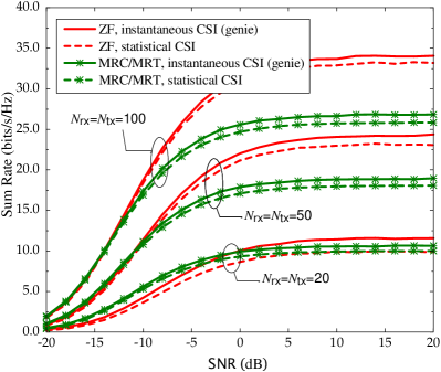
Figure 2: Sum rate versus $\mathsf{SNR}$ for ZF and MRC/MRT processing ($K=10$, $\tau=2K$, and $\sigma_{\tt LI}^{2}=1$).

The problem (58) is equivalent to

$$\left.\begin{array}[]{l}\text{minimize}\hskip 14.22636pt\sum_{k=1}^{K}p_{{\tt S},k}+p_{\tt{R}}\\ \text{subject to}\hskip 14.22636pt\frac{T-\tau}{T}\sum_{k=1}^{K}\log_{2}\left(1+\gamma_{k}\right)=\mathcal{S}^{\tt A}_{0}\\ \hskip 62.59596pt\gamma_{k}\leq\frac{a_{k}p_{{\tt S},k}}{\sum_{j=1}^{K}b_{j}p_{{\tt S},j}+c_{k}p_{\tt{R}}+1},k=1,...,K\\ \hskip 62.59596pt\gamma_{k}\leq\frac{d_{k}p_{\tt{R}}}{e_{k}p_{\tt{R}}+1},k=1,...,K\\ \hskip 64.01869pt0\leq p_{{\tt S},k}\leq p_{0},k=1,...,K\\ \hskip 64.01869pt0\leq p_{\tt{R}}\leq p_{1}.\\ \end{array}\right.$$ (65)

Since $a_{k}$, $b_{k}$, $c_{k}$, $d_{k}$, and $e_{k}$ are positive, (65) can be equivalently written as

$$\left.\begin{array}[]{l}\text{minimize}\hskip 14.22636pt\sum_{k=1}^{K}p_{{\tt S},k}+p_{\tt{R}}\\ \text{subject to}\hskip 14.22636pt\prod_{k=1}^{K}\left(1+\gamma_{k}\right)=2^{\frac{T\mathcal{S}^{\tt A}_{0}}{T-\tau}}\\ \hskip 14.22636pt\sum\limits_{j=1}^{K}\!\!\frac{b_{j}}{a_{k}}p_{{\tt S},j}\gamma_{k}p_{{\tt S},k}^{-1}\!+\!\frac{c_{k}}{a_{k}}p_{\tt{R}}\gamma_{k}p_{{\tt S},k}^{-1}+\frac{1}{a_{k}}\gamma_{k}p_{{\tt S},k}^{-1}\leq 1,\forall k\\ \hskip 14.22636pt\frac{e_{k}}{d_{k}}\gamma_{k}+\frac{1}{d_{k}}\gamma_{k}p_{\tt{R}}^{-1}\leq 1,k=1,...,K\\ \hskip 14.22636pt0\leq p_{{\tt S},k}\leq p_{0},k=1,...,K,\\ \hskip 14.22636pt0\leq p_{\tt{R}}\leq p_{1}.\\ \end{array}\right.$$ (72)

We can see that the objective function and the inequality constraints are posynomial functions. If the equality constraint is a monomial function, the problem (72) becomes a GP which can be reformulated as a convex problem, and can be solved efficiently by using convex optimization tools, such as CVX [27]. However, the equality constraint in (72) is a posynomial function, so we cannot solve (72) directly using convex optimization tools. Yet, by using the technique in [28], we can efficiently find an approximate solution of (72) by solving a sequence of GPs. More precisely, from [28, Lemma 1], we can use $\kappa_{k}\gamma_{k}^{\eta_{k}}$ to approximate $1+\gamma_{k}$ near a point $\hat{\gamma}_{k}$, where $\eta_{k}\triangleq\hat{\gamma}_{k}\left(1+\hat{\gamma}_{k}\right)^{-1}$ and $\kappa_{k}\triangleq\hat{\gamma}_{k}^{-\eta_{k}}\left(1+\hat{\gamma}_{k}\right)$. As a consequence, near a point $\hat{\gamma}_{k}$, the left hand side of the equality constraint can be approximated as

$$\prod_{k=1}^{K}\left(1+\gamma_{k}\right)\approx\prod_{k=1}^{K}\kappa_{k}\gamma_{k}^{\eta_{k}},$$ (73)

which is a monomial function. Thus, by using the local approximation given by (73), the optimization problem (72) can be approximated by a GP. By using a similar technique as in [28], we formulate the following algorithm to solve (72):

Algorithm 1 (Successive approximation algorithm for (72))

1.

Initialization: set $i=1$, choose the initial values of $\gamma_{k}$ as $\gamma_{k,1}$, $k=1,...,K$. Define a tolerance $\epsilon$, the maximum number of iterations $L$, and parameter $\alpha$.

2.

Iteration $i$: compute $\eta_{k,i}={\gamma}_{k,i}\left(1+{\gamma}_{k,i}\right)^{-1}$ and $\kappa_{k,i}={\gamma}_{k,i}^{-\eta_{k,i}}\left(1+{\gamma}_{k,i}\right)$. Then, solve the GP:

$$\left.\begin{array}[]{l}\text{minimize}\hskip 14.22636pt\sum_{k=1}^{K}p_{{\tt S},k}+p_{\tt{R}}\\ \text{subject to}\hskip 14.22636pt\prod_{k=1}^{K}\kappa_{k,i}\gamma_{k}^{\eta_{k,i}}=2^{\frac{T\mathcal{S}^{\tt A}_{0}}{T-\tau}}\\ \hskip 5.69046pt\sum\limits_{j=1}^{K}\!\!\frac{b_{j}}{a_{k}}p_{{\tt S},j}\gamma_{k}p_{{\tt S},k}^{-1}\!+\!\frac{c_{k}}{a_{k}}p_{\tt{R}}\gamma_{k}p_{{\tt S},k}^{-1}\!+\!\frac{1}{a_{k}}\gamma_{k}p_{{\tt S},k}^{-1}\leq 1,\forall k\\ \hskip 5.69046pt\frac{e_{k}}{d_{k}}\gamma_{k}+\frac{1}{d_{k}}\gamma_{k}p_{\tt{R}}^{-1}\leq 1,k=1,...,K\\ \hskip 5.69046pt0\leq p_{{\tt S},k}\leq p_{0},k=1,...,K,~{}0\leq p_{\tt{R}}\leq p_{1}\\ \hskip 5.69046pt\alpha^{-1}\gamma_{k,i}\leq\gamma_{k}\leq\alpha\gamma_{k,i}\\ \end{array}\right.$$

Let $\gamma_{k}^{\ast}$, $k=1,...,K$ be the solutions.

3.

If $\max_{k}\left|\gamma_{k,i}-\gamma_{k}^{\ast}\right|<\epsilon$ or $i=L$ $\rightarrow$ Stop. Otherwise, go to step 4.

4.

Set $i=i+1$, $\gamma_{k,i}=\gamma_{k}^{\ast}$, go to step 2.

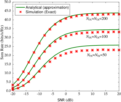
Figure 3: Sum rate versus $\mathsf{SNR}$ for ZF processing ($K=10$, $\tau=2K$, and $\sigma_{\tt LI}^{2}=1$).

Note that the parameter $\alpha>1$ is used to control the approximation accuracy in (73). If $\alpha$ is close to $1$, the accuracy is high, but the convergence speed is low and vice versa if $\alpha$ is large. As discussed in [28], $\alpha=1.1$ offers a good accuracy and convergence speed tradeoff.

VI Numerical Results

In all illustrative examples, we choose the length of the coherence interval to be $T=200$ (symbols), the number of communication pairs $K=10$, the training length $\tau=2K$, and $N_{\mathrm{tx}}=N_{\mathrm{rx}}$. Furthermore, we define $\mathsf{SNR}\triangleq p_{\tt{S}}$.

VI-A Validation of Achievable Rate Results

In this subsection, we evaluate the validity of our achievable rate given by (26) as well as the approximation used to derive the closed-form expression given in Theorem 1. We choose the loop interference level $\sigma_{\tt LI}^{2}=1$. We assume that $p_{\mathrm{p}}=p_{\tt{S}}$, and that the total transmit power of the $K$ sources is equal to the transmit power of the relay station, i.e., $p_{\tt{R}}=Kp_{\tt{S}}$.

We first compare our achievable rate given by (26), where the destination uses the statistical distributions of the channels (i.e., the means of channel gains) to detect the transmitted signal, with the one obtained by (34), where we assume that there is a genie receiver (instantaneous CSI) at the destination. Figure 2 shows the sum rate versus $\mathsf{SNR}$ for ZF and MRC/MRT processing. The dashed lines represent the sum rates obtained numerically from (26), while the solid lines represent the ergodic sum rates obtained from (34). We can see that the relative performance gap between the cases with instantaneous (genie) and statistical CSI at the destinations is small. For example, with $N_{\mathrm{rx}}=N_{\mathrm{tx}}=50$, at $\mathsf{SNR}=5$dB, the sum-rate gaps are 0.65 bits/s/Hz and 0.9 bits/s/Hz for MRC/MRT and ZF processing, respectively. This implies that using the mean of the effective channel gain for signal detection is fairly reasonable, and the achievable rate given in (26) is a good predictor of the system performance.

Next, we evaluate the validity of the approximation given by (1). Figure 3 shows the sum rate versus $\mathsf{SNR}$ for different numbers of transmit (receive) antennas. The “Analytical (approximation)” curves are obtained by using Theorem 1, and the “Simulation (exact)” curves are generated from the outputs of a Monte-Carlo simulator using (26), (29), and (33). We can see that the proposed approximation is very tight, especially for large antenna arrays.

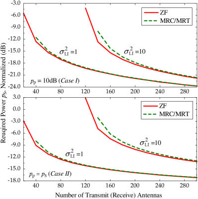
Figure 4: Transmit power, $p_{\tt{S}}$, required to achieve 1 bit/channel use per user for ZF and MRC/MRT processing ($K=10$, $\tau=2K$, and $p_{\tt{R}}=Kp_{\tt{S}}$).

VI-B Power Efficiency

We now examine the power efficiency of using large antenna arrays for two cases: $p_{\mathrm{p}}$ is fixed (Case I) and $p_{\mathrm{p}}=p_{\tt{S}}$ (Case II). We will examine how much transmit power is needed to reach a predetermined sum spectral efficiency. We set $p_{\tt{R}}=Kp_{\tt{S}}$ and $\beta_{{\tt SR},k}=\beta_{{\tt RD},k}=1$, $k=1,2,...,K$. Figure 4 shows the required transmit power, $p_{\tt{S}}$, to achieve $1$ bits/s/Hz per communication pair. We can see that when the number of antennas increases, the required transmit powers are significantly reduced. As predicted by the analysis, in the large-antenna regime, we can cut back the power by approximately $3$dB and $1.5$dB by doubling the number of antennas for Case I and Case II, respectively. When the loop interference is high and the number of antennas is moderate, the power efficiency can benefit more by increasing the number of antennas. For instance, for $\sigma_{\tt LI}^{2}=10$, increasing the number of antennas from $120$ to $240$ yields a power reduction of $15$dB and $13$dB for Case I and Case II, respectively. Regarding the loop interference effect, when $\sigma_{\tt LI}^{2}$ increases, we need more transmit power. However, when $\sigma_{\tt LI}^{2}$ is high and the number of antennas is small, even if we use infinite transmit power, we cannot achieve a required sum spectral efficiency. Instead of this, we can add more antennas to reduce the loop interference effect and achieve the required QoS. Furthermore, when the number of antennas is large, the difference in performance between ZF and MRC/MRT processing is negligible.

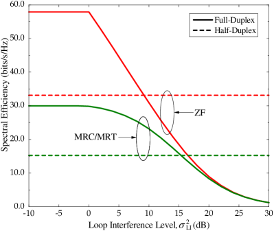
Figure 5: Sum spectral efficiency versus the loop interference levels for half-duplex and full-duplex relaying ($K=10$, $\tau=2K$, $p_{\tt{R}}=p_{\mathrm{p}}=p_{\tt{S}}=10$dB, and $N_{\mathrm{tx}}=N_{\mathrm{rx}}=100$).

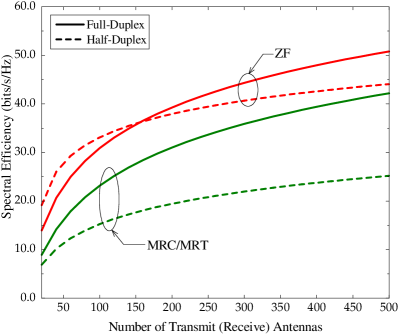
Figure 6: Sum spectral efficiency versus the number of transmit (receive) antennas for half-duplex and full-duplex relaying ($K=10$, $\tau=2K$, $p_{\tt{R}}=p_{\mathrm{p}}=p_{\tt{S}}=10$dB, and $\sigma_{\tt LI}^{2}=10$dB).

VI-C Full-Duplex Vs. Half-Duplex, Hybrid Relaying Mode

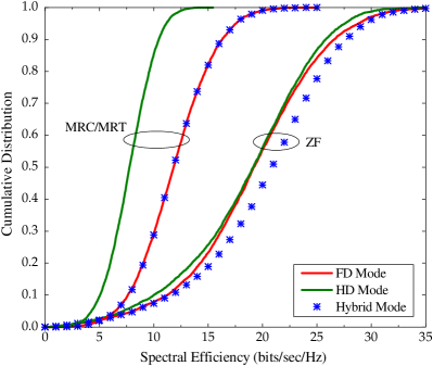
Figure 7: Cumulative distribution of the sum spectral efficiency for half-duplex, full-duplex, and Hybrid relaying ($K=10$, $\tau=2K$, $p_{\tt{R}}=p_{\mathrm{p}}=p_{\tt{S}}=10$dB, and $\sigma_{\tt LI}^{2}=10$dB).

Firstly, we compare the performance between half-duplex and full-duplex relaying for different loop interference levels, $\sigma_{\tt LI}^{2}$. We choose $p_{\tt{R}}=p_{\mathrm{p}}=p_{\tt{S}}=10$dB, $\beta_{{\tt SR},k}=\beta_{{\tt RD},k}=1$, $\forall k$, and $N_{\mathrm{rx}}=N_{\mathrm{tx}}=100$. Figure 5 shows the sum spectral efficiency versus the loop interference levels for ZF and MRC/MRT. As expected, at low $\sigma_{\tt LI}^{2}$, full-duplex relaying outperforms half-duplex relaying. This gain is due to the larger pre-log factor (one) of the full-duplex mode. However, when $\sigma_{\tt LI}^{2}$ is high, loop interference dominates the system performance of the full-duplex mode and, hence, the performance of the half-duplex mode is superior. In this case, by using larger antenna arrays at the relay station, we can reduce the effect of the loop interference and exploit the larger pre-log factor of the full-duplex mode. This fact is illustrated in Fig. 6 where the sum spectral efficiency is represented as a function of the number of antennas, at $\sigma_{\tt LI}^{2}=10$dB.

We next consider a more practical scenario that incorporates small-scale fading and large-scale fading. The large-scale fading is modeled by path loss, shadow fading, and random source and destination locations. More precisely, the large-scale fading $\beta_{{\tt SR},k}$ is

$$\beta_{{\tt SR},k}=\frac{z_{{\tt SR},k}}{1+\left(\ell_{k}/\ell_{0}\right)^{\nu}},$$

where $z_{{\tt SR},k}$ represents a log-normal random variable with standard deviation of $\sigma$dB, $\nu$ is the path loss exponent, $\ell_{k}$ denotes the distance between ${\tt S}_{k}$ and the receive array of the relay station, and $\ell_{0}$ is a reference distance. We use the same channel model for $\beta_{{\tt RD},k}$.

We assume that all sources and destinations are located uniformly at random inside a disk with a diameter of $1000$m. For our simulation, we choose $\sigma=8$dB, $\nu=3.8$, $\ell_{0}=200$m, which are typical values in an urban cellular environment [29]. Furthermore, we choose $N_{\mathrm{rx}}=N_{\mathrm{tx}}=200$, $p_{\tt{R}}=p_{\mathrm{p}}=p_{\tt{S}}=10$dB, and $\sigma_{\tt LI}^{2}=10$dB. Figure 7 illustrates the cumulative distributions of the sum spectral efficiencies for the half-duplex, full-duplex, and hybrid modes. The ZF processing outperforms the MRC/MRT processing in this example, and the sum spectral efficiency of MRC/MRT processing is more concentrated around its mean compared to the ZF processing. Furthermore, we can see that, for MRC/MRT, the full-duplex mode is always better than the half-duplex mode, while for ZF, depending on the large-scale fading, full-duplex can be better than half-duplex relaying and vice versa. In this example, it is also shown that relaying using the hybrid mode provides a large gain for the ZF processing case.

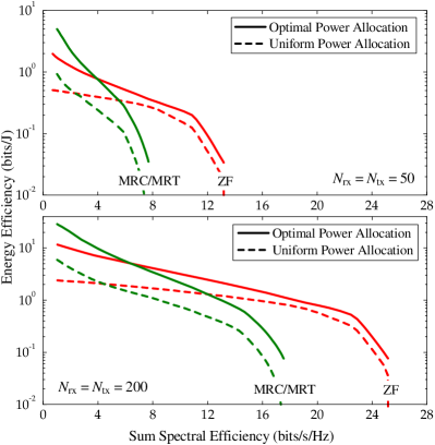
Figure 8: Energy efficiency versus sum spectral efficiency for ZF and MRC/MRT ($K=10$, $\tau=2K$, $p_{\mathrm{p}}=10$dB, and $\sigma_{\tt LI}^{2}=10$dB).

VI-D Power Allocation

In the following, we will examine the energy efficiency versus the sum spectral efficiency under the optimal power allocation, as outlined in Section V-C. In this example, we choose $p_{\mathrm{p}}=10$dB and $\sigma_{\tt LI}^{2}=10$dB. Furthermore, the large-scale fading matrices are chosen as follows:

$${\mathbf{D}}_{\tt SR} =\mathrm{diag}\left[0.749~{}0.246~{}0.125~{}0.635~{}4.468\right.$$

$$\hskip 99.58464pt\left.0.031~{}0.064~{}0.257~{}0.195~{}0.315\right],$$

$${\mathbf{D}}_{\tt RD} =\mathrm{diag}\left[0.070~{}0.121~{}0.134~{}0.209~{}0.198\right.$$

$$\hskip 99.58464pt\left.0.184~{}0.065~{}0.051~{}0.236~{}1.641\right].$$

Note that, the above large-scale coefficients are obtained by taking one snapshot of the practical setup for Fig. 7.

Figure 8 shows the energy efficiency versus sum the spectral efficiency under uniform and optimal power allocation. The “uniform power allocation” curves correspond to the case where all sources and the relay station use their maximum powers, i.e., $p_{{\tt S},k}=p_{0}$, $\forall k=1,...,K$, and $p_{\tt{R}}=p_{1}$. The “optimal power allocation” curves are obtained by using the optimal power allocation scheme via Algorithm 1. The initial values of Algorithm 1 are chosen as follows: $\epsilon=0.01$, $L=5$, $\alpha=1.1$, and $\gamma_{k,1}=\min\left\{\frac{a_{k}p_{0}}{p_{0}\sum_{j=1}^{K}b_{j}+c_{k}p_{1}+1},\frac{d_{k}p_{1}}{e_{k}p_{1}+1}\right\}$ which correspond to the uniform power allocation case. We can see that with optimal power allocation, the system performance improves significantly, especially at low spectral efficiencies. For example, with $N_{\mathrm{rx}}=N_{\mathrm{tx}}=200$, to achieve the same sum spectral efficiency of $10$bits/s/Hz, optimal power allocation can improve the energy efficiency by factors of $2$ and $3$ for ZF and MRC/MRT processing, respectively, compared to the case of no power allocation. This manifests that MRC/MRT processing benefits more from power allocation. Furthermore, at low spectral efficiencies, MRC/MRT performs better than ZF and vice versa at high spectral efficiencies. The results also demonstrate the significant benefit of using large antenna arrays at the relay station. With ZF processing, by increasing the number of antennas from $50$ to $200$, the energy efficiency can be increased by $14$ times, when each pair has a throughput of about one bit per channel use.

VII Conclusion

In this paper, we introduced and analyzed a multipair full-duplex relaying system, where the relay station is equipped with massive arrays, while each source and destination have a single antenna. We assume that the relay station employs ZF and MRC/MRT to process the signals. The analysis takes the energy and bandwidth costs of channel estimation into account. We show that, by using massive arrays at the relay station, loop interference can be canceled out. Furthermore, the interpair interference and noise disappear. As a result, massive MIMO can increase the sum spectral efficiency by $2K$ times compared to the conventional orthogonal half-duplex relaying, and simultaneously reduce the transmit power significantly. We derived closed-form expressions for the achievable rates and compared the performance of the full-duplex and half-duplex modes. In addition, we proposed a power allocation scheme which chooses optimally the transmit powers of the $K$ sources and of the relay station to maximize the energy efficiency, subject to a given sum spectral efficiency and peak power constraints. With the optimal power allocation, the energy efficiency can be significantly improved.

-A Proof of Proposition 1

1. For ZF processing:

   Here, we first provide the proof for ZF processing. From (7) and (13), we have

   $$\sqrt{p_{\tt{S}}}{\mathbf{W}}^{T}{\mathbf{G}}_{\tt SR}{\mathbf{x}}\left[i\right] \!=\!\sqrt{p_{\tt{S}}}{\mathbf{W}}_{\tt ZF}^{T}\left(\hat{{\mathbf{G}}}_{\tt SR}+\boldsymbol{\mathcal{E}}_{\tt SR}\right){\mathbf{x}}\left[i\right]$$

   $$\!=\!\sqrt{p_{\tt{S}}}{\mathbf{x}}\left[i\right]\!+\!\sqrt{p_{\tt{S}}}{\mathbf{W}}_{\tt ZF}^{T}\boldsymbol{\mathcal{E}}_{\tt SR}{\mathbf{x}}\left[i\right].$$ (74)

   By using the law of large numbers, we obtain

   $$\sqrt{p_{\tt{S}}}{\mathbf{W}}_{\tt ZF}^{T}\boldsymbol{\mathcal{E}}_{\tt SR}{\mathbf{x}}\left[i\right] =\sqrt{p_{\tt{S}}}\left(\frac{\hat{{\mathbf{G}}}_{\tt SR}^{H}\hat{{\mathbf{G}}}_{\tt SR}}{N_{\mathrm{rx}}}\right)^{-1}\frac{\hat{{\mathbf{G}}}_{\tt SR}^{H}\boldsymbol{\mathcal{E}}_{\tt SR}}{N_{\mathrm{rx}}}{\mathbf{x}}\left[i\right]$$

   $$\mathop{\to}\limits^{a.s.}0,~{}\text{as}~{}N_{\mathrm{rx}}\to\infty.$$ (75)

   Therefore, as $N_{\mathrm{rx}}\to\infty$, we have

   $$\sqrt{p_{\tt{S}}}{\mathbf{W}}^{T}{\mathbf{G}}_{\tt SR}{\mathbf{x}}\left[i\right]\mathop{\to}\limits^{a.s.}\sqrt{p_{\tt{S}}}{\mathbf{x}}\left[i\right].$$ (76)

   From (76), we can see that, when $N_{\mathrm{rx}}$ goes to infinity, the desired signal converges to a deterministic value, while the multi-pair interference is cancelled out. More precisely, as $N_{\mathrm{rx}}\to\infty$,

   $$\sqrt{p_{\tt{S}}}{\mathbf{w}}_{k}^{T}{\mathbf{g}}_{{\tt SR},k}{x}_{k}\left[i\right] \mathop{\to}\limits^{a.s.}\sqrt{p_{\tt{S}}}{x}_{k}\left[i\right],$$ (77)

   $$\sqrt{p_{\tt{S}}}{\mathbf{w}}_{k}^{T}{\mathbf{g}}_{{\tt SR},j}{x}_{j}\left[i\right] \mathop{\to}\limits^{a.s.}0,~{}\forall j\neq k.$$ (78)

   Next, we consider the loop interference. With ZF processing, we have

   $$\sqrt{p_{\tt{R}}}{\mathbf{W}}^{T}{\mathbf{G}}_{\tt RR}{\mathbf{s}}\left[i\right] =\alpha_{\tt ZF}\sqrt{p_{\tt{R}}}\left(\frac{\hat{{\mathbf{G}}}_{\tt SR}^{H}\hat{{\mathbf{G}}}_{\tt SR}}{N_{\mathrm{rx}}}\right)^{-1}$$

   $$\!\times\!\frac{\hat{{\mathbf{G}}}_{\tt SR}^{H}{\mathbf{G}}_{\tt RR}\hat{{\mathbf{G}}}_{\tt RD}^{\ast}}{N_{\mathrm{rx}}N_{\mathrm{tx}}}\left(\!\frac{\hat{{\mathbf{G}}}_{\tt RD}^{T}\hat{{\mathbf{G}}}_{\tt RD}^{\ast}}{N_{\mathrm{tx}}}\!\right)^{-1}\!\!\!{\mathbf{x}}\left[i\!-\!d\right].$$ (79)

   If $N_{\mathrm{tx}}$ is fixed, then it is obvious that $\sqrt{p_{\tt{R}}}{\mathbf{W}}^{T}{\mathbf{G}}_{\tt RR}{\mathbf{s}}\left[i\right]\to 0$, as $N_{\mathrm{rx}}\to\infty$. We now consider the case where $N_{\mathrm{tx}}$ and $N_{\mathrm{rx}}$ tend to infinity with a fixed ratio. The $(m,n)$th element of the $K\times K$ matrix $\alpha_{\tt ZF}\frac{\hat{{\mathbf{G}}}_{\tt SR}^{H}{\mathbf{G}}_{\tt RR}\hat{{\mathbf{G}}}_{\tt RD}^{\ast}}{N_{\mathrm{rx}}N_{\mathrm{tx}}}$ can be written as

   $$\alpha_{\tt ZF}\!\frac{\hat{{\mathbf{g}}}_{{\tt SR},m}^{H}\!{\mathbf{G}}_{\tt RR}\hat{{\mathbf{g}}}_{{\tt RD},n}^{\ast}}{N_{\mathrm{rx}}N_{\mathrm{tx}}}\!\!=\!\!\sqrt{\frac{N_{\mathrm{tx}}-K}{N_{\mathrm{tx}}\!\!\sum\limits_{k=1}^{K}\!\!\sigma_{{\tt RD},k}^{-2}}}\frac{1}{N_{\mathrm{rx}}}\!\hat{{\mathbf{g}}}_{{\tt SR},m}^{H}\!\frac{{\mathbf{G}}_{\tt RR}\hat{{\mathbf{g}}}_{{\tt RD},n}^{\ast}}{\sqrt{N_{\mathrm{tx}}}}.$$ (80)

   We can see that the vector $\frac{{\mathbf{G}}_{\tt RR}\hat{{\mathbf{g}}}_{{\tt RD},n}^{\ast}}{\sqrt{N_{\mathrm{tx}}}}$ includes i.i.d. zero-mean random variables with variance $\sigma_{{\tt RD},n}^{2}\sigma_{\tt LI}^{2}$. This vector is independent of the vector $\hat{{\mathbf{g}}}_{{\tt SR},m}$. Thus, by using the law of large numbers, we can obtain

   $$\alpha_{\tt ZF}\!\frac{\hat{{\mathbf{g}}}_{{\tt SR},m}^{H}\!{\mathbf{G}}_{\tt RR}\hat{{\mathbf{g}}}_{{\tt RD},n}^{\ast}}{N_{\mathrm{rx}}N_{\mathrm{tx}}}\mathop{\to}\limits^{a.s.}0,~{}\text{as}~{}N_{\mathrm{rx}}\!\to\!\infty,N_{\mathrm{rx}}/N_{\mathrm{tx}}~{}\text{is fixed}.$$ (81)

   Therefore, the loop interference converges to $0$ when $N_{\mathrm{rx}}$ grows without bound. Similarly, we can show that

   $${\mathbf{W}}^{T}{\mathbf{n}}_{\tt R}\left[i\right]\mathop{\to}\limits^{a.s.}0.$$ (82)

   Substituting (77), (78), (81), and (82) into (II-B1), we arrive at (19).

2. For MRC/MRT processing:

   We next provide the proof for MRC/MRT processing. From (7) and (16), and by using the law of large numbers, as $N_{\mathrm{rx}}\to\infty$, we have that

   $$\frac{1}{N_{\mathrm{rx}}}\sqrt{p_{\tt{S}}}{\mathbf{w}}_{k}^{T}{\mathbf{g}}_{{\tt SR},k}{x}_{k}\left[i\right] =\frac{1}{N_{\mathrm{rx}}}\sqrt{p_{\tt{S}}}\hat{{\mathbf{g}}}_{{\tt SR},k}^{H}{\mathbf{g}}_{{\tt SR},k}{x}_{k}\left[i\right]$$

   $$\mathop{\to}\limits^{a.s.}\sqrt{p_{\tt{S}}}\sigma_{{\tt SR},k}^{2}{x}_{k}\left[i\right],$$ (83)

   $$\frac{1}{N_{\mathrm{rx}}}\sqrt{p_{\tt{S}}}{\mathbf{w}}_{K}^{T}{\mathbf{g}}_{{\tt SR},j}{x}_{k}\left[j\right] =\frac{1}{N_{\mathrm{rx}}}\sqrt{p_{\tt{S}}}\hat{{\mathbf{g}}}_{{\tt SR},k}^{H}{\mathbf{g}}_{{\tt SR},j}{x}_{k}\left[j\right]$$

   $$\mathop{\to}\limits^{a.s.}0,~{}\forall j\neq k.$$ (84)

   We next consider the loop interference. For any finite $N_{\mathrm{tx}}$, or any $N_{\mathrm{tx}}$ where $N_{\mathrm{rx}}/N_{\mathrm{tx}}$ is fixed, as $N_{\mathrm{rx}}\to\infty$, we have

   $$\frac{1}{N_{\mathrm{rx}}}\sqrt{p_{\tt{R}}}{\mathbf{W}}^{T}{\mathbf{G}}_{\tt RR}{\mathbf{s}}\left[i\right] =\alpha_{\tt MRT}\sqrt{p_{\tt{R}}}\frac{\hat{{\mathbf{G}}}_{\tt SR}^{H}{\mathbf{G}}_{\tt RR}\hat{{\mathbf{G}}}_{\tt RD}^{\ast}}{N_{\mathrm{rx}}}{\mathbf{x}}\left[i-d\right]$$

   $$\mathop{\to}\limits^{a.s.}0,$$ (85)

   where the convergence follows a similar argument as in the proof for ZF processing. Similarly, we can show that

   $$\frac{1}{N_{\mathrm{rx}}}{\mathbf{w}}_{k}^{T}{\mathbf{n}}_{\tt R}\left[i\right]\mathop{\to}\limits^{a.s.}0.$$ (86)

   Substituting (2), (84), (2), and (86) into (II-B1), we obtain (20).

-B Proof of Theorem 1

-B1 Derive $R_{{\tt SR}_{k}}$

From (29), we need to compute $\operatorname{\mathtt{E}}\left\{{\mathbf{w}}_{k}^{T}{\mathbf{g}}_{{\tt SR},k}\right\}$, $\operatorname{\mathbb{V}\mathrm{ar}}\left({\mathbf{w}}_{k}^{T}{\mathbf{g}}_{{\tt SR},k}\right)$, ${\tt MP}_{k}$, ${\tt LI}_{k}$, and ${\tt AN}_{k}$.

• Compute $\operatorname{\mathtt{E}}\left\{{\mathbf{w}}_{k}^{T}{\mathbf{g}}_{{\tt SR},k}\right\}$:

  Since, ${\mathbf{W}}^{T}=\left(\hat{{\mathbf{G}}}_{\tt SR}^{H}\hat{{\mathbf{G}}}_{\tt SR}\right)^{-1}\hat{{\mathbf{G}}}_{\tt SR}^{H}$, from (7), we have

  $${\mathbf{W}}^{T}{{\mathbf{G}}}_{\tt SR}={\mathbf{W}}^{T}\left(\hat{{\mathbf{G}}}_{\tt SR}+\boldsymbol{\mathcal{E}}_{\tt SR}\right)={\mathbf{I}}_{N_{\mathrm{rx}}}+{\mathbf{W}}^{T}\boldsymbol{\mathcal{E}}_{\tt SR}.$$ (87)

  Therefore,

  $${\mathbf{w}}_{k}^{T}{{\mathbf{g}}}_{{\tt SR},k}=1+{\mathbf{w}}_{k}^{T}\boldsymbol{\varepsilon}_{{\tt SR},k}$$ (88)

  where $\boldsymbol{\varepsilon}_{{\tt SR},k}$ is the $k$th column of $\boldsymbol{\mathcal{E}}_{\tt SR}$. Since $\boldsymbol{\varepsilon}_{{\tt SR},k}$ and ${\mathbf{w}}_{k}$ are uncorrelated, and $\boldsymbol{\varepsilon}_{{\tt SR},k}$ is a zero-mean random variable, $\operatorname{\mathtt{E}}\left\{{\mathbf{w}}_{k}^{T}\boldsymbol{\varepsilon}_{{\tt SR},k}\right\}=0$. Thus,

  $$\operatorname{\mathtt{E}}\left\{{\mathbf{w}}_{k}^{T}{\mathbf{g}}_{{\tt SR},k}\right\}=1.$$ (89)

• Compute $\operatorname{\mathbb{V}\mathrm{ar}}\left({\mathbf{w}}_{k}^{T}{\mathbf{g}}_{{\tt SR},k}\right)$:

  From (88) and (89), the variance of ${\mathbf{w}}_{k}^{T}{\mathbf{g}}_{{\tt SR},k}$ is given by

  $$\operatorname{\mathbb{V}\mathrm{ar}}\left({\mathbf{w}}_{k}^{T}{\mathbf{g}}_{{\tt SR},k}\right) =\operatorname{\mathtt{E}}\left\{\left|{\mathbf{w}}_{k}^{T}\boldsymbol{\varepsilon}_{{\tt SR},k}\right|^{2}\right\}$$

  $$=\left(\beta_{{\tt SR},k}-\sigma_{{\tt SR},k}^{2}\right)\operatorname{\mathtt{E}}\left\{\left\|{\mathbf{w}}_{k}\right\|^{2}\right\}$$

  $$=\left(\beta_{{\tt SR},k}\!-\!\sigma_{{\tt SR},k}^{2}\right)\!\operatorname{\mathtt{E}}\left\{\!\left[\left(\hat{{\mathbf{G}}}_{\tt SR}^{H}\hat{{\mathbf{G}}}_{\tt SR}\right)^{-1}\right]_{kk}\!\right\}$$

  $$=\frac{\beta_{{\tt SR},k}-\sigma_{{\tt SR},k}^{2}}{\sigma_{{\tt SR},k}^{2}K}\operatorname{\mathtt{E}}\left\{\operatorname{\mathrm{tr}}\left({\mathbf{X}}^{-1}\right)\right\}$$

  $$=\frac{\beta_{{\tt SR},k}-\sigma_{{\tt SR},k}^{2}}{\sigma_{{\tt SR},k}^{2}}\frac{1}{N_{\mathrm{rx}}-K},~{}\text{for}~{}N_{\mathrm{rx}}>K,$$ (90)

  where ${\mathbf{X}}$ is a $K\times K$ central Wishart matrix with $N_{\mathrm{rx}}$ degrees of freedom and covariance matrix ${\mathbf{I}}_{K}$, and the last equality is obtained by using [30, Lemma 2.10].

• Compute ${\tt MP}_{k}$:

  From (87), we have that ${\mathbf{w}}_{k}^{T}{{\mathbf{g}}}_{{\tt SR},j}={\mathbf{w}}_{k}^{T}\boldsymbol{\varepsilon}_{{\tt SR},j}$, for $j\neq k$. Since ${\mathbf{w}}_{k}$ and $\boldsymbol{\varepsilon}_{{\tt SR},j}$ are uncorrelated, we obtain

  $$\operatorname{\mathtt{E}}\left\{\left|{\mathbf{w}}_{k}^{T}\boldsymbol{\varepsilon}_{{\tt SR},j}\right|^{2}\right\} =\left(\beta_{{\tt SR},j}-\sigma_{{\tt SR},j}^{2}\right)\operatorname{\mathtt{E}}\left\{\left\|{\mathbf{w}}_{k}\right\|^{2}\right\}$$

  $$=\frac{\beta_{{\tt SR},j}-\sigma_{{\tt SR},j}^{2}}{\sigma_{{\tt SR},k}^{2}}\frac{1}{N_{\mathrm{rx}}-K}.$$ (91)

  Therefore,

  $${\tt MP}_{k}=p_{\tt{S}}\sum_{j\neq K}^{K}\frac{\beta_{{\tt SR},j}-\sigma_{{\tt SR},j}^{2}}{\sigma_{{\tt SR},k}^{2}}\frac{1}{N_{\mathrm{rx}}-K}.$$ (92)

• Compute ${\tt LI}_{k}$:

  From (31), with ZF, the LI can be rewritten as

  $${\tt LI}_{k} =p_{\tt{R}}\operatorname{\mathtt{E}}\left\{{\mathbf{w}}_{k}^{T}{\mathbf{G}}_{\tt RR}{\mathbf{A}}_{\tt ZF}{\mathbf{A}}_{\tt ZF}^{H}{\mathbf{G}}_{\tt RR}^{H}{\mathbf{w}}_{k}^{\ast}\right\}.$$ (93)

  From (14), we have

  $${\mathbf{A}}_{\tt ZF}{\mathbf{A}}_{\tt ZF}^{H}=\alpha_{\tt ZF}^{2}\hat{{\mathbf{G}}}_{\tt RD}^{\ast}\left(\hat{{\mathbf{G}}}_{\tt RD}^{T}\hat{{\mathbf{G}}}_{\tt RD}^{\ast}\right)^{-1}\left(\hat{{\mathbf{G}}}_{\tt RD}^{T}\hat{{\mathbf{G}}}_{\tt RD}^{\ast}\right)^{-1}\hat{{\mathbf{G}}}_{\tt RD}^{T}.$$ (94)

  When $N_{\mathrm{tx}}\gg K$, we can use the law of large numbers to obtain the following approximation:

  $$\hat{{\mathbf{G}}}_{\tt RD}^{T}\hat{{\mathbf{G}}}_{\tt RD}^{\ast}\approx N_{\mathrm{tx}}\hat{{\mathbf{D}}}_{\tt RD},$$ (95)

  where $\hat{{\mathbf{D}}}_{\tt RD}$ is a $K\times K$ diagonal matrix whose $(k,k)$th element is $\left[\hat{{\mathbf{D}}}_{\tt RD}\right]_{kk}=\sigma_{{\tt RD},k}^{2}$. Therefore,

  $${\mathbf{A}}_{\tt ZF}{\mathbf{A}}_{\tt ZF}^{H}\approx\frac{\alpha_{\tt ZF}^{2}}{N_{\mathrm{tx}}^{2}}\hat{{\mathbf{G}}}_{\tt RD}^{\ast}\hat{{\mathbf{D}}}_{\tt RD}^{-2}\hat{{\mathbf{G}}}_{\tt RD}^{T}.$$ (96)

  Substituting (96) into (93) we obtain

  $${\tt LI}_{k} \approx p_{\tt{R}}\frac{\alpha_{\tt ZF}^{2}}{N_{\mathrm{tx}}^{2}}\operatorname{\mathtt{E}}\left\{{\mathbf{w}}_{k}^{T}{\mathbf{G}}_{\tt RR}\hat{{\mathbf{G}}}_{\tt RD}^{\ast}\hat{{\mathbf{D}}}_{\tt RD}^{-2}\hat{{\mathbf{G}}}_{\tt RD}^{T}{\mathbf{G}}_{\tt RR}^{H}{\mathbf{w}}_{k}^{\ast}\right\}$$

  $$=p_{\tt{R}}\frac{\alpha_{\tt ZF}^{2}}{N_{\mathrm{tx}}^{2}}\left(\sum_{j=1}^{K}\frac{1}{\sigma_{{\tt RD},j}^{2}}\right)\operatorname{\mathtt{E}}\left\{{\mathbf{w}}_{k}^{T}{\mathbf{G}}_{\tt RR}{\mathbf{G}}_{\tt RR}^{H}{\mathbf{w}}_{k}^{\ast}\right\}$$

  $$=p_{\tt{R}}\frac{\alpha_{\tt ZF}^{2}\sigma_{\tt LI}^{2}}{N_{\mathrm{tx}}}\left(\sum_{j=1}^{K}\frac{1}{\sigma_{{\tt RD},j}^{2}}\right)\operatorname{\mathtt{E}}\left\{\left\|{\mathbf{w}}_{k}\right\|^{2}\right\}$$

  $$=\frac{\sigma_{\tt LI}^{2}p_{\tt{R}}\left(N_{\mathrm{tx}}-K\right)}{\sigma_{{\tt SR},k}^{2}N_{\mathrm{tx}}\left(N_{\mathrm{rx}}-K\right)}.$$ (97)

• Compute ${\tt AN}_{k}$:

  Similarly, we obtain

  $${\tt AN}_{k}=\frac{1}{\sigma_{{\tt SR},k}^{2}}\frac{1}{N_{\mathrm{rx}}-K}.$$ (98)

Substituting (89), (• ‣ -B1), (92), (• ‣ -B1), and (98) into (29), we obtain

$$R_{{\tt SR},k}\!\approx\!\log_{2}\!\left(\!1\!+\!\frac{p_{\tt{S}}\left(N_{\mathrm{rx}}-K\right)\sigma_{{\tt SR},k}^{2}}{p_{\tt{S}}\sum\limits_{j=1}^{K}\!\!\left(\beta_{{\tt SR},j}\!-\!\sigma_{{\tt SR},j}^{2}\!\right)\!+\!p_{\tt{R}}\!\sigma_{\tt LI}^{2}\left(\!1\!-\!\frac{K}{N_{\mathrm{tx}}}\!\right)\!+\!1}\right).$$ (99)

-B2 Derive $R_{{\tt RD},k}$

From (33), to derive $R_{{\tt RD},k}$, we need to compute $\operatorname{\mathtt{E}}\left\{{\mathbf{g}}_{{\tt RD},k}^{T}{\mathbf{a}}_{k}\right\}$, $\operatorname{\mathbb{V}\mathrm{ar}}\left({\mathbf{g}}_{{\tt RD},k}^{T}{\mathbf{a}}_{k}\right)$, and $\operatorname{\mathtt{E}}\left\{\left|{\mathbf{g}}_{{\tt RD},k}^{T}{\mathbf{a}}_{j}\right|^{2}\right\}$. Following the same methodology as the one used to compute $\operatorname{\mathtt{E}}\left\{{\mathbf{w}}_{k}^{T}{\mathbf{g}}_{{\tt SR},k}\right\}$, $\operatorname{\mathbb{V}\mathrm{ar}}\left({\mathbf{w}}_{k}^{T}{\mathbf{g}}_{{\tt SR},k}\right)$, and ${\tt MP}_{k}$, we obtain

$$\operatorname{\mathtt{E}}\left\{{\mathbf{g}}_{{\tt RD},k}^{T}{\mathbf{a}}_{k}\right\} =\alpha_{\tt ZF},$$ (100)

$$\operatorname{\mathbb{V}\mathrm{ar}}\left({\mathbf{g}}_{{\tt RD},k}^{T}{\mathbf{a}}_{k}\right) =\frac{\left(\beta_{{\tt RD},k}-\sigma_{{\tt RD},k}^{2}\right)\alpha_{\tt ZF}^{2}}{\sigma_{{\tt RD},k}^{2}\left(N_{\mathrm{tx}}-K\right)},$$ (101)

$$\operatorname{\mathtt{E}}\left\{\left|{\mathbf{g}}_{{\tt RD},k}^{T}{\mathbf{a}}_{j}\right|^{2}\right\} =\frac{\left(\beta_{{\tt RD},k}-\sigma_{{\tt RD},k}^{2}\right)\alpha_{\tt ZF}^{2}}{\sigma_{{\tt RD},j}^{2}\left(N_{\mathrm{tx}}-K\right)},~{}\text{for}~{}j\neq k.$$ (102)

Substituting (100)–(102) into (33), we obtain a closed-form expression for $R_{{\tt RD},k}$:

$$R_{{\tt RD},k}=\log_{2}\left(1+\frac{N_{\mathrm{tx}}-K}{\sum_{j=1}^{K}\sigma_{{\tt RD},j}^{-2}}\frac{p_{\tt{R}}}{p_{\tt{R}}\left(\beta_{{\tt RD},k}-\sigma_{{\tt RD},k}^{2}\right)+1}\right).$$ (103)

Then, using (26), (99), and (103), we arrive at (1).

-C Proof of Theorem 2

With MRC/MRT processing, ${\mathbf{W}}^{T}=\hat{{\mathbf{G}}}_{\tt SR}^{H}$ and ${\mathbf{A}}=\alpha_{\tt MRT}\hat{{\mathbf{G}}}_{\tt RD}^{\ast}$.

1. Compute $\operatorname{\mathtt{E}}\left\{{\mathbf{w}}_{k}^{T}{\mathbf{g}}_{{\tt SR},k}\right\}$:

   We have

   $${\mathbf{w}}_{k}^{T}{{\mathbf{g}}}_{{\tt SR},k}=\hat{{\mathbf{g}}}_{{\tt SR},k}^{H}{\mathbf{g}}_{{\tt SR},k}=\left\|\hat{{\mathbf{g}}}_{{\tt SR},k}\right\|^{2}+\hat{{\mathbf{g}}}_{{\tt SR},k}^{H}\boldsymbol{\varepsilon}_{{\tt SR},k}.$$ (104)

   Therefore,

   $$\operatorname{\mathtt{E}}\left\{{\mathbf{w}}_{k}^{T}{\mathbf{g}}_{{\tt SR},k}\right\}=\operatorname{\mathtt{E}}\left\{\left\|\hat{{\mathbf{g}}}_{{\tt SR},k}\right\|^{2}\right\}=\sigma_{{\tt SR},k}^{2}N_{\mathrm{rx}}.$$ (105)

2. Compute $\operatorname{\mathbb{V}\mathrm{ar}}\left({\mathbf{w}}_{k}^{T}{\mathbf{g}}_{{\tt SR},k}\right)$:

   From (104) and (105), the variance of ${\mathbf{w}}_{k}^{T}{\mathbf{g}}_{{\tt SR},k}$ is given by

   $$\operatorname{\mathbb{V}\mathrm{ar}}\left({\mathbf{w}}_{k}^{T}{\mathbf{g}}_{{\tt SR},k}\right)=\operatorname{\mathtt{E}}\left\{\left|{\mathbf{w}}_{k}^{T}{\mathbf{g}}_{{\tt SR},k}\right|^{2}\right\}-\sigma_{{\tt SR},k}^{4}N_{\mathrm{rx}}^{2}$$

   $$=\operatorname{\mathtt{E}}\left\{\left|\left\|\hat{{\mathbf{g}}}_{{\tt SR},k}\right\|^{2}+\hat{{\mathbf{g}}}_{{\tt SR},k}^{H}\boldsymbol{\varepsilon}_{{\tt SR},k}\right|^{2}\right\}-\sigma_{{\tt SR},k}^{4}N_{\mathrm{rx}}^{2}$$

   $$=\operatorname{\mathtt{E}}\left\{\left\|\hat{{\mathbf{g}}}_{{\tt SR},k}\right\|^{4}\right\}+\operatorname{\mathtt{E}}\left\{\left|\hat{{\mathbf{g}}}_{{\tt SR},k}^{H}\boldsymbol{\varepsilon}_{{\tt SR},k}\right|^{2}\right\}-\sigma_{{\tt SR},k}^{4}N_{\mathrm{rx}}^{2}.$$ (106)

   By using [30, Lemma 2.9], we obtain

   $$\operatorname{\mathbb{V}\mathrm{ar}}\left({\mathbf{w}}_{k}^{T}{\mathbf{g}}_{{\tt SR},k}\right) =\sigma_{{\tt SR},k}^{4}N_{\mathrm{rx}}\left(N_{\mathrm{rx}}+1\right)$$

   $$+\sigma_{{\tt SR},k}^{2}\left(\beta_{{\tt SR},k}-\sigma_{{\tt SR},k}^{2}\right)N_{\mathrm{rx}}-\sigma_{{\tt SR},k}^{4}N_{\mathrm{rx}}^{2}$$

   $$=\sigma_{{\tt SR},k}^{2}\beta_{{\tt SR},k}N_{\mathrm{rx}}.$$ (107)

3. Compute ${\tt MP}_{k}$:

   For $j\neq k$, we have

   $$\operatorname{\mathtt{E}}\left\{\left|{\mathbf{w}}_{k}^{T}{\mathbf{g}}_{{\tt SR},j}\right|^{2}\right\}=\operatorname{\mathtt{E}}\left\{\left|\hat{{\mathbf{g}}}_{{\tt SR},k}^{H}{\mathbf{g}}_{{\tt SR},j}\right|^{2}\right\}=\sigma_{{\tt SR},k}^{2}\beta_{{\tt SR},j}N_{\mathrm{rx}}.$$ (108)

   Therefore,

   $${\tt MP}_{k}=p_{\tt{S}}\sigma_{{\tt SR},k}^{2}N_{\mathrm{rx}}\sum_{j\neq k}^{K}\beta_{{\tt SR},j}.$$ (109)

4. Compute ${\tt LI}_{k}$:

   Since $\hat{{\mathbf{g}}}_{{\tt SR},k}$, ${\mathbf{G}}_{\tt RR}$, and $\hat{{\mathbf{G}}}_{\tt RD}$ are independent, we obtain

   $${\tt LI}_{k} =\alpha_{\tt MRT}^{2}p_{\tt{R}}\operatorname{\mathtt{E}}\left\{\hat{{\mathbf{g}}}_{{\tt SR},k}^{H}{\mathbf{G}}_{\tt RR}\hat{{\mathbf{G}}}_{\tt RD}^{\ast}\hat{{\mathbf{G}}}_{\tt RD}^{T}{\mathbf{G}}_{\tt RR}^{H}\hat{{\mathbf{g}}}_{{\tt SR},k}^{\ast}\right\}$$

   $$=\alpha_{\tt MRT}^{2}p_{\tt{R}}\left(\sum_{j=1}^{K}\sigma_{{\tt RD},j}^{2}\right)\operatorname{\mathtt{E}}\Big{\{}\hat{{\mathbf{g}}}_{{\tt SR},k}^{H}{\mathbf{G}}_{\tt RR}{\mathbf{G}}_{\tt RR}^{H}\hat{{\mathbf{g}}}_{{\tt SR},k}^{\ast}\Big{\}}$$

   $$=\alpha_{\tt MRT}^{2}p_{\tt{R}}\left(\sum_{j=1}^{K}\sigma_{{\tt RD},j}^{2}\right)\sigma_{\tt LI}^{2}N_{\mathrm{tx}}\operatorname{\mathtt{E}}\Big{\{}\hat{{\mathbf{g}}}_{{\tt SR},k}^{H}\hat{{\mathbf{g}}}_{{\tt SR},k}^{\ast}\Big{\}}$$

   $$=p_{\tt{R}}\sigma_{\tt LI}^{2}\sigma_{{\tt SR},k}^{2}N_{\mathrm{rx}}.$$ (110)

5. Compute ${\tt AN}_{k}$:

   Similarly, we obtain

   $${\tt AN}_{k}=\sigma_{{\tt SR},k}^{2}N_{\mathrm{rx}}.$$ (111)

Substituting (105), (2), (109), (4), and (111) into (29), we obtain

$$R_{{\tt SR},k}=\log_{2}\left(1+\frac{p_{\tt{S}}N_{\mathrm{rx}}\sigma_{{\tt SR},k}^{2}}{p_{\tt{S}}\sum_{j=1}^{K}\beta_{{\tt SR},j}+p_{\tt{R}}\sigma_{\tt LI}^{2}+1}\right).$$ (112)

Similarly, we obtain a closed-form expression for $R_{{\tt RD},k}$, and then we arrive at (2).

References

• [1] H. Q. Ngo, H. A. Suraweera, M. Matthaiou, and E. G. Larsson, “Multipair massive MIMO full-duplex relaying with MRC/MRT processing,” in Proc. IEEE Int. Conf. Commun. (ICC), 2014.
• [2] T. L. Marzetta, “Noncooperative cellular wireless with unlimited numbers of base station antennas,” IEEE Trans. Wireless Commun., vol. 9, no. 11, pp. 3590–3600, Nov. 2010.
• [3] F. Rusek, D. Persson, B. K. Lau, E. G. Larsson, T. L. Marzetta, O. Edfors, and F. Tufvesson, “Scaling up MIMO: Opportunities and challenges with very large arrays,” IEEE Signal Process. Mag., vol. 30, no. 1, pp. 40–60, Jan. 2013.
• [4] E. G. Larsson, F. Tufvesson, O. Edfors, and T. L. Marzetta, “Massive MIMO for next generation wireless systems,” IEEE Commun. Mag., vol. 52, no. 2, pp. 186–195 , Feb. 2014.
• [5] H. A. Suraweera, H. Q. Ngo, T. Q. Duong, C. Yuen, and E. G. Larsson, “Multi-pair amplify-and-forward relaying with very large antenna arrays,” in Proc. IEEE Int. Conf. Commun. (ICC), June 2013, pp. 3228-3233.
• [6] D. W. Bliss, P. A. Parker, and A. R. Margetts, “Simultaneous transmission and reception for improved wireless network performance,” in Proc. IEEE Workshop Statist. Signal Process. (SSP), Aug. 2007, pp. 478–482.
• [7] D. W. Bliss, T. Hancock and P. Schniter, “Hardware and environmental phenomenological limits on full-duplex MIMO relay performance,” in Proc. Annual Asilomar Conf. Signals, Syst., Comput., Nov. 2012.
• [8] T. Riihonen, S. Werner, and R. Wichman, “Mitigation of loopback self-interference in full-duplex MIMO relays,” IEEE Trans. Signal Process., vol. 59, no. 12, pp. 5983–5993, Dec. 2011.
• [9] —, “Hybrid full-duplex/half-duplex relaying with transmit power adaptation,” IEEE Trans. Wireless Commun., vol. 10, no. 9, pp. 3074–3085, Sep. 2011.
• [10] —, “Transmit power optimization for multiantenna decode-and-forward relays with loopback self-interference from full-duplex operation,” in Proc. Annual Asilomar Conf. Signals, Syst., Comput., Nov. 2011, pp 1408–1412.
• [11] G. Zheng, I. Krikidis, and B. Ottersten, “Full-duplex cooperative cognitive radio with transmit imperfections,” IEEE Trans. Wireless Commun., vol. 12, no. 5, pp. 2498-2511, May 2013.
• [12] E. Aryafar, M. A. Khojastepour, K. Sundaresan, S. Rangarajan, and M. Chiang, “MIDU: Enabling MIMO full duplex,” in Proc. ACM Int. Conf. Mobile Comput. Netw. (MobiCom), Aug. 2012.
• [13] M. Duarte, Full-duplex wireless: Design, implementation and characterization.   Rice University, Houston, TX: Ph.D. dissertation, 2012.
• [14] M. Duarte, A. Sabharwal, V. Aggarwal, R. Jana, K. Ramakrishnan, C. Rice, and N. Shankaranarayanan, “Design and characterization of a full-duplex multi-antenna system for WiFi networks.” [Online]. Available: http://arxiv. org/abs/1210.1639.
• [15] Y. Sung, J. Ahn, B. V. Nguyen and K. Kim, “Loop-interference suppression strategies using antenna selection in full-duplex MIMO relays,” in Proc. Int. Symp. Intelligent Signal Process. and Commun. Syst. (ISPACS 2011), Dec. 2011.
• [16] H. A. Suraweera, I. Krikidis, and C. Yuen, “Antenna selection in the full-duplex multi-antenna relay channel,” in Proc. IEEE Int. Conf. Commun. (ICC), June 2013, pp. 3416–3421.
• [17] W. Zhang, X. Ma, B. Gestner, and D. V. Anderson, “Designing low-complexity equalizers for wireless systems,” IEEE Comm. Mag., vol. 47, pp. 56-62, Jan. 2009.
• [18] Z. Zhao, Z. Ding, M. Peng, W. Wang, and K. K. Leung, “A special case of multi-way relay channel: When beamforming is not applicable,” IEEE Trans. Wireless Commun., vol. 10, no. 7, pp. 2046-2051, July 2011.
• [19] Y. Yang, H. Hu, J. Xu, and G. Mao, “Relay technologies for WiMAX and LTE-advanced mobile systems,” IEEE Commun. Mag., vol 47, no 10, pp. 100-105, Oct. 2009.
• [20] X. Gao, O. Edfors, F. Rusek, and F. Tufvesson, “Linear pre-coding performance in measured very-large MIMO channels,” in Proc. IEEE Veh. Technol. Conf. (VTC), Sept. 2011.
• [21] S. M. Kay, Fundamentals of Statistical Signal Processing: Estimation Theory.   Englewood Cliffs, NJ: Prentice Hall, 1993.
• [22] H. Q. Ngo, E. G. Larsson, and T. L. Marzetta, “Energy and spectral efficiency of very large multiuser MIMO systems,” IEEE Trans. Commun., vol. 61, no. 4, pp. 1436-1449, April 2013.
• [23] H. Yang and T. L. Marzetta, “Performance of conjugate and zero-forcing beamforming in large-scale antenna systems,” IEEE J. Sel. Areas Commun., vol. 31, no. 2, pp. 172–179, Feb. 2013.
• [24] B. Hassibi and B. M. Hochwald, “How much training is needed in multiple-antenna wireless links?” IEEE Trans. Inf. Theory, vol. 49, no. 4, pp. 951–963, Apr. 2003.
• [25] J. Jose, A. Ashikhmin, T. L. Marzetta, and S. Vishwanath, “Pilot contamination and precoding in multi-cell TDD systems,” IEEE Trans. Wireless Commun., vol. 10, no. 8, pp. 2640–2651, Aug. 2011.
• [26] A. Pitarokoilis, S. K. Mohammed, and E. G. Larsson, “On the optimality of single-carrier transmission in large-scale antenna systems,” IEEE Wireless Commun. Lett., vol. 1, no. 4, pp. 276–279. Aug. 2012.
• [27] S. Boyd and L. Vandenberghe, Convex Optimization.   Cambridge, UK: Cambridge University Press, 2004.
• [28] P. C. Weeraddana, M. Codreanu, M. Latva-aho, and A. Ephremides, “Resource allocation for cross-layer utility maximization in wireless networks,” IEEE Trans. Veh. Technol., vol. 60, no. 6, pp. 2790–2809, July 2011.
• [29] W. Choi and J. G. Andrews, “The capacity gain from intercell scheduling in multi-antenna systems,” IEEE Trans. Wireless Commun., vol. 7, no. 2, pp. 714–725, Feb. 2008.
• [30] A. M. Tulino and S. Verdú, “Random matrix theory and wireless communications,” Foundations and Trends in Communications and Information Theory, vol. 1, no. 1, pp. 1–182, Jun. 2004.