ALiCCE: Atomic Lines Calibration using the Cross-Entropy Algorithm

Abstract

Atomic line opacities play a crucial role in stellar astrophysics. They strongly modify the radiative transfer in stars, therefore impacting their physical structure. Ultimately, most of our knowledge of stellar population systems (stars, clusters, galaxies, etc.) relies on the accuracy with which we understand and reproduce the stellar spectra. With such a wide impact on Astronomy, it would be ideal to have access to a complete, accurate and precise list of atomic transitions. This, unfortunately, is not the case. Few atomic transitions had their parameters actually measured in the laboratory, and for most of the lines the parameters were calculated with low precision atomic energy levels. Only a small fraction of the lines were calibrated empirically. For the purpose of computing a stellar spectral grid with a complete coverage of spectral types and luminosity classes, this situation is rather limiting. We have implemented an innovative method to perform a robust calibration of atomic line lists used by spectral synthesis codes called ALiCCE: Atomic Lines Calibration using the Cross-Entropy algorithm. Here we describe the implementation and validation of the method, using synthetic spectra which simulates the signal-to-noise, spectral resolution and rotational velocities typical of high quality observed spectra. We conclude that the method is efficient for calibrating atomic line lists.

1 Introduction

Atomic line opacities play a crucial role in stellar astrophysics. First, they strongly modify the radiative transfer in stars, and therefore impact their physical structure. Secondly, the detailed comparison between model and observed spectra is a powerful diagnostic tool that may be used to study stars and stellar populations. Everything we know about the chemical abundances on stars, planets, galaxies, interstellar, intergalactic and intracluster medium is, ultimately, dependent on the quantum mechanic parameters which characterize atomic (and molecular) electronic (vibrational and rotational) transitions. These parameters will, given the thermodynamic conditions in which the transition happens, define the profile of the spectral line. For the case of atomic transitions, these parameters are: the central wavelength of the line, the energy levels of the transition, the oscillator strength (which dominates the line depth) and the broadening parameters (which dominate the wings of the lines).

With such a wide impact on Astronomy, one would expect by now to have access to a complete, accurate and precise list of atomic transitions. This, unfortunately, is not the case. Although nowadays there exist fairly comprehensive databases (e.g., the NIST Atomic Spectra Database  and the Vienna Atomic Line Database ) of the atomic transition probabilities necessary for stellar abundance studies, they are far from being complete.

In general, one half the discernible lines in observed stellar spectra are missing from the line lists with good wavelengths (Kurucz, 2011). To have an accurate opacity list for atoms and ions, we need all levels, including hyperfine and isotopic splittings. Lifetimes and damping constants depend on sums over the levels. Inside stars there are thermal and density cutoffs that limit the number of levels, but in circumstellar, interstellar, and intergalactic space, photoionization and recombination can populate high levels, even for high ions. We need all stages of ionization for elements at least up through Zn. In the Sun there are unidentified asymmetric triangular features that are unresolved multiplets of light elements (Kurucz, 2011). All the magnetic dipole, electric quadrupole, and maybe higher-pole, forbidden lines are required as well. However, except for the simplest species, it is impossible to generate accurate energy levels or wavelengths theoretically. In principle, they must be measured in the laboratory.

Because the parameters of relatively few lines were actually measured in laboratory, to compute a theoretical stellar spectra with good spectrophotometry is necessary to include the so-called “predicted lines”: lines where either one or both energy levels of the transition were predicted from quantum mechanics calculations (Kurucz, 1992). Usually only the lower energy levels of atoms have been determined in the laboratory, particularly for complex spectra such as those from iron. If only those transitions were taken into account, the atmospheric line blanketing computed from such data would be severely incomplete. The predicted lines are essential for computing accurately the structure of model atmospheres and for spectrophotometric predictions (e.g. Short & Lester, 1996). But as the quantum mechanics predictions are accurate to only a few per cent, wavelengths for these lines may be largely uncertain. Also the line oscillator strengths are sufficiently accurate merely in a statistical sense. The predicted lines are, therefore, unsuitable for high resolution analyses (Bell et al., 1994; Castelli & Kurucz, 2004; Munari et al., 2005).

Efforts are underway to reduce transition probability uncertainties of selected lines (e.g. Taklif, 1990; Klose et al., 2002; Fuhr & Wiese, 2006; Safronova & Safronova, 2010; Bacławski, 2011; Pickering et al., 2011; Wiese et al., 2011; Civiš et al., 2012; Ruffoni et al., 2013) and accurately compute broadening parameters (e.g. Anstee & O’Mara, 1995; Barklem & O’Mara, 1997; Barklem et al., 1998; Lesage et al., 1999; Barklem et al., 2000; Konjević et al., 2002; Derouich et al., 2003; Dimitrijević et al., 2003). Also, for the purpose of high spectral resolution chemical analysis of stellar photospheres, several limitations of the atomic line lists are being successfully tackled by different authors and methods (e.g. Stalin et al., 1997; Blackwell-Whitehead et al., 2008; Borrero et al., 2003; Jorissen, 2004; Sobeck et al., 2007; Meléndez & Barbuy, 2009; Wahlgren, 2010; Den Hartog et al., 2011; Shchukina & Vasil’eva, 2013; Wood et al., 2013).

It has also been shown in the literature (e.g. Barbuy et al., 2003; Martins & Coelho, 2007) that even empirical calibrations of some specific lines can produce significant improvement on the synthetic spectra generated. The empirical calibration is done by changing the values of the parameters on the line list, generating models and comparing them with observations of very well known stars (like the Sun or Arcturus, for example). This process is repeated until the results are adequate (Barbuy et al., 2003).

Nevertheless, these approaches tend to improve the quality of a selective group lines, mostly those that were considered more suitable to chemical abundance measurements, where relatively weak lines in the linear part of the curve of growth are favored. On the other hand, the strong lines close to saturation and blended features are the ones which dominate spectral indices in integrated spectra of stellar populations.

While these efforts are improving the parameters for thousands of lines, tens of millions of lines are estimated to be needed to compute, say, a complete stellar grid with a good range of atmospheric parameters. Therefore, an innumerous amount of lines remain poorly characterized. For the ultimate goal of computing a large grid of theoretical stellar spectra for further use in automatic classification of stellar spectroscopic surveys and stellar population modeling, this is rather limiting.

Aiming to overcome these limitations and to create a more robust and automatic method for the calibration of atomic parameters, we introduce a powerful statistical technique recently developed to deal with multi-extremal problems involving optimization: the cross-entropy algorithm (hereafter, CE).

In this work we validate our CE method to calibrate atomic line lists using synthetic spectra which simulates very well known stars. The code is hereafter called ALiCCE: Atomic Lines Calibration using the Cross-Entropy algorithm. We show the great capability of the method to determine the atomic parameters of the absorption lines by comparing the models with the simulated spectra. This paper is structured as follows: in §2 we explain the Cross-Entropy method, in §3 we explain the methodology used in the validation process, in §4 we show our results and in §5 we present our discussion and conclusion.

2 The Cross-Entropy Method and ALiCCE

To compute a synthetic stellar spectrum, the spectral synthesis code reads a model atmosphere, and a list of molecular and atomic transitions. From the many model atmospheres available in the literature we choose the library from (Castelli & Kurucz, 2004) which is based on ATLAS9 (Kurucz, 1970; Sbordone et al., 2004). This is an extensive grid of models and according to Martins & Coelho (2007) it is one that in average, reproduces well the colors of observed stars.

To generate the synthetic spectra we chose the code SYNTHE (Kurucz & Avrett, 1981) in its public Linux port by Sbordone et al. (2004). SYNTHE reads the atomic and molecular transition lines in separated files. The atomic lines are listed in files which are publicly distributed with SYNTHE.

The synthesis codes use the atomic line lists to solve the continuum radiative transfer equation and to determine the absorption lines formation. The parameters needed for the computation of each line profile are: the central wavelength, the transition levels energy, the oscillator strength $\log(gf)$ (which is related to the line intensity) and the broadening parameters (natural - $\log~{}\Gamma_{rad}$, Stark - $\log~{}\Gamma_{StarK}$ and Van der Waals - $\log\Gamma_{vdW}$ broadening). Broadening parameters are responsible for the line profile. The natural broadening comes directly from the Heisenberg’s uncertainty principle of quantum mechanics: because an electron that finds itself in an energy level has a finite lifetime before transitioning to a lower energy level, the energy levels have a certain width $\Delta E$, resulting in a width of the atomic line. The radiative damping constant $\Gamma_{rad}$ is then equal to the sum of the reciprocal of the mean lifetimes of the two atomic energy levels under consideration. Another mode of line broadening is the pressure (or collisional) broadening, which is due to the perturbation of the potential of the atom by neighboring particles. For example, the Stark effect is caused by the splitting of degenerate atomic energy levels due to the presence of an external electric field, or a frequency shift for these levels. Another example of pressure broadening is the Van der Waals process, which is related to the perturbation of an atom’s potential by neutral atoms electric dipole. Their definition implies that the Stark process will be more important for hotter stars while the Van der Waals will be more important for cooler stars.

In the present work we choose to calibrate the oscillator strength and the two pressure broadenings - Stark and Van der Waals.

Another detail we have to consider to calibrate the lines is that although the same line list is used to generate the spectra of all stars, not every line will be present in all stellar spectra. The intensity and the profile of each absorption feature is determined by the physical conditions of the stellar atmosphere where the lines are formed. Lines originated from the lowest ionization degrees will be more intense in cooler stars. On the other hand, lines originated from higher ionization degrees will be stronger on the spectrum of hotter stars. Many other physical parameters can also change the intensity and the profile of the lines, like chemical abundances, gravity, etc. Besides, many lines are blended in the spectrum of a star, which makes it very hard to disentangle the atomic parameters of each line. Ideally, in order to be able to calibrate all the lines in a given line list one would have to attempt to calibrate the lists to a variety of stellar spectral types simultaneously. In different spectral types, the relative intensity of each line in a blend might be different. Calibrating the line list to all of them simultaneously would better constraint the best solution.

2.1 The Cross-Entropy Algorithm

For the task of calibrating the atomic line list we adapted the CE algorithm. The CE method is a general Monte Carlo approach to combinatorial and continuous multi-extremal optimization and importance sampling, which is a general technique for estimating properties of a particular distribution, using samples generated randomly from a different statistical distribution rather than the distribution of interest.

The CE analysis was originally used in the optimization of complex computer simulation models involving rare events simulations (Rubinstein, 1997), where very small probabilities have to be accurately estimated, having been modified by Rubinstein (1999) to deal with continuous multi-extremal and discrete combinatorial optimization problems. Its theoretical asymptotic convergence has been demonstrated by Margolin (2004), while Kroese et al. (2006) studied the efficiency of the CE method in solving continuous multi-extremal optimization problems. Some examples of robustness of the CE method in several situations are listed in de Boer et al. (2005). The CE procedure uses concepts of importance sampling, which is a variance reduction technique, but removing the need for a priory knowledge of the reference parameters of the parent distribution. The CE procedure provides a simple adaptive way of estimating the optimal reference parameters.

The CE method was already used successfully in astrophysical problems like the study of sources with jet precession (Caproni et al., 2009, 2013), fitting the color-magnitude diagram of open clusters (Monteiro et al., 2010; Oliveira et al., 2013) and modeling very long baseline interferometric images (Caproni et al., 2011).

The basic procedures involved in the CE optimization can be summarized as follows (e.g. Kroese et al., 2006):

(i) Random generation of the initial parameter sample, obeying predefined criteria;

(ii) Selection of the best samples based on some mathematical criterion;

(iii) Random generation of updated parameter samples from the previous best candidates to be evaluated in the next iteration;

(iv) Optimization process that repeats steps (ii) and (iii) until a pre-specified stopping criterion is fulfilled.

Let us suppose that we wish to study a set of $N_{\mathrm{d}}$ observational data in terms of an analytical model characterized by $N_{\mathrm{p}}$ parameters $p_{1},p_{2},...,p_{N_{\mathrm{p}}}$.

The main goal of the CE continuous multi-extremal optimization method is to find the set of parameters ${\bf x}^{*}=(p^{*}_{1},p^{*}_{2},...,p^{*}_{Np})$ for which the model provides the best description of the data (Rubinstein, 1999; Kroese et al., 2006). In our case $N_{\mathrm{d}}$ is the number of stellar spectra we are trying to reproduce, and ${N_{\mathrm{p}}}$ is three times the number of lines in the interval calibrated (because we are calibrating three parameters for each line). The technique is performed by generating randomly $N$ independent sets of model parameters ${\bf X}=({\bf x}_{1},{\bf x}_{2},...,{\bf x}_{N})^{T}$, where ${\bf x}_{i}=(p_{1i},p_{2i},...,p_{N{\mathrm{p}i}})$, and minimizing an objective function $S({\bf x})$ used to transmit the quality of the fit during the run process. If the convergence to the exact solution is achieved then $S({\bf x}^{*})\rightarrow 0$.

In order to find the optimal solution from CE optimization, we start by defining the parameter range in which the algorithm will search for the best candidates: $p^{\mathrm{min}}_{j}\leq p_{j}(k)\leq p^{\mathrm{max}}_{j}$, where $k$ represents the iteration number. Introducing $\bar{p}_{j}(0)=(p^{\mathrm{min}}_{j}+p^{\mathrm{max}}_{j})/2$ and $\sigma_{j}(0)=(p^{\mathrm{max}}_{j}-p^{\mathrm{min}}_{j})/2$, we can compute ${\bf X}(0)$ from:

$$X_{ij}(0)=\bar{p}_{j}(0)+\sigma_{j}(0)G_{ij},$$ (1)

where $G_{ij}$ is an $N\times N_{\mathrm{p}}$ matrix with random numbers generated from a zero-mean normal distribution with standard deviation of unity.

The next step is to calculate $S_{i}(0)$ for each set of ${\bf x}_{i}(0)$, ordering them according to increasing values of $S_{i}$. Then the first $N_{\mathrm{elite}}$ set of parameters is selected, i.e. the $N_{\mathrm{elite}}$-samples with lowest $S$-values, which will be labeled as the elite sample array ${\bf X}^{\mathrm{elite}}(0)$.

We then determine the mean and standard deviation of the elite sample, $\bar{p}^{\mathrm{elite}}_{j}(0)$ and ${\bf\sigma}^{\mathrm{elite}}_{j}(0)$ respectively, as:

$$\bar{p}^{\mathrm{elite}}_{j}(0)=\frac{1}{N_{\mathrm{elite}}}\sum\limits_{i=1}^{N_{\mathrm{elite}}}X^{\mathrm{elite}}_{ij}(0),$$ (2)

$${\bf\sigma}^{\mathrm{elite}}_{j}(0)=\sqrt{\frac{1}{\left(N_{\mathrm{elite}}-1\right)}\sum\limits_{i=1}^{N_{\mathrm{elite}}}\left[X^{\mathrm{elite}}_{ij}(0)-\bar{p}^{\mathrm{elite}}_{j}(0)\right]^{2}}.$$ (3)

The array ${\bf X}$ at the next iteration is determined as:

$$X_{ij}(1)=\bar{p}^{\mathrm{elite}}_{j}(0)+{\bf\sigma}^{\mathrm{elite}}_{j}(0)G_{ij},$$ (4)

This process is repeated from equation (2), with $G_{ij}$ regenerated at each iteration. The optimization stops when either the mean value of ${\bf\sigma}^{\mathrm{elite}}_{i}(k)$ is smaller than a predefined value or the maximum number of iterations $k_{\mathrm{max}}$ is reached. In our case the stopping criteria is always $k_{\mathrm{max}}$, as will be explained in section 4.

In order to prevent convergence to a sub-optimal solution due to the intrinsic rapid convergence of the CE method, Kroese et al. (2006) suggested the implementation of a fixed smoothing scheme for ${\bf\sigma}^{\mathrm{elite,s}}_{j}(k)$:

$${\bf\sigma}^{\mathrm{elite,s}}_{j}(k)=\alpha_{\mathrm{d}}(k){\bf\sigma}^{\mathrm{elite}}_{j}(k)+\left[1-\alpha_{\mathrm{d}}(k)\right]{\bf\sigma}^{\mathrm{elite}}_{j}(k-1),$$ (5)

where $\alpha_{\mathrm{d}}(k)$ is a dynamic smoothing parameter at $k$th iteration:

$$\alpha_{\mathrm{d}}(k)=\alpha-\alpha\left(1-k^{-1}\right)^{q},$$ (6)

with $0<\alpha<1$ and $q$ is an integer typically between 5 and 10 (Kroese et al., 2006).

As mentioned before, such parametrization prevents the algorithm from finding a non-global minimum solution since it guarantees polynomial speed of convergence instead of exponential (Kroese et al., 2006).

2.2 The performance function

In order to select the best model that represents our observation we need to define a performance function, based on the desired characteristics of the solution. Usually, for continuous problems this is done by defining a likelihood function and then maximizing it, or alternatively requiring that the sum of the squared residuals be minimal.

In this work the performance function has to be defined as a way to compare model with observed spectra pixel by pixel. For this comparison we choose as a performance function the combination of the sum of the squared residuals and their respective variance, as suggested in Caproni et al. (2011).

Let the quadratic residual $R_{m}(k)$ at a given wavelength pixel $m$ and iteration $k$ be defined as the squared difference between the observed spectrum we want to reproduce, $I_{m}$, and the generated model spectrum $M_{m}(k)$ at a $k$-iteration, i.e. $R_{m}(k)=[I_{m}-M_{m}(k)]^{2}$. The mean square residual value of the model fitting $\bar{R}(k)$ can be calculated from:

$$\bar{R}(k)=\frac{1}{N_{\mathrm{pixel}}}\left[\sum\limits_{m=1}^{N_{\mathrm{pixel}}}R_{m}(k)\right].$$ (7)

As mentioned in the previous section, we need the spectra of stars spanning a range of effective temperatures (T_eff), surface gravities($\log{g}$) and metallicity in order to guarantee that lines to be calibrate will be present in at least one spectrum. Considering $N_{\mathrm{s}}$ as the number of stars used in the calibration, our tentative model spectra obtained from the $N_{\mathrm{s}}$ parameters ${\bf x}_{i}(k)$ at iteration $k$ are ranked through the performance function:

$$S_{\mathrm{prod}}({\bf x}_{i},k)=\prod_{j=1}^{N_{S}}\bar{R}(k)\times\frac{1}{N_{\mathrm{pixel}}}\left[\sum\limits_{m=1}^{N_{\mathrm{pixel}}}\left(R_{m}(k)-\bar{R}(k)\right)^{2}\right],$$ (8)

which corresponds to the product of individual merit functions associated with the $N_{\mathrm{s}}$ stars used in the calibration. The product of these functions is important to ensure that high luminosity stars do not become more important than low luminosity stars. Note also that, if $I_{m}$ and $M_{m}$ are expressed in terms of ergs cm²Å^-1, $S_{\mathrm{prod}}$ has units of (ergs cm²Å${}^{-1})^{6N_{S}}$.

It is important to emphasize that we have tested other functional forms for the CE performance function (as a root mean square, for example) but Equation (8) was more efficient to recover the best solution for our problem. As mentioned by Caproni et al. (2011), the difference in performance is essentially due to the fact that Equation (8) transmits directly any change in the mean and variance of the residuals in all iteration steps of the optimization process.

2.3 Determination of the parameters and their uncertainties

As commented previously, CE optimization generates $N$ random tentative solutions at each iteration $k$, selecting the best $N_{\mathrm{elite}}$ set of model parameters in terms of the values of $S_{\mathrm{prod}}$.

If the stopping criteria is related to a maximum number of iterations, the last iteration might not be exactly the one with the best $S_{\mathrm{prod}}$. The best values of the parameters $p_{i}^{*}$, as well as their respective uncertainties $\sigma_{p_{i}^{*}}$, were then determined as follows:

$$p_{i}^{*}=\sum\limits_{k=1}^{k_{\mathrm{conv}}}w_{k}p_{ik}\left(\sum\limits_{k=1}^{k_{\mathrm{conv}}}w_{k}\right)^{-1}$$ (9)

and

$$\sigma_{p^{*}_{i}}^{2}=\sum\limits_{k=1}^{k_{\mathrm{conv}}}w_{k}\left(p_{ik}-p^{*}_{i}\right)^{2}\left(\sum\limits_{k=1}^{k_{\mathrm{conv}}}w_{k}\right)^{-1},$$ (10)

where $k_{\mathrm{conv}}$ is the iteration where the parameter converged, and $p_{ik}$ represents the set of model parameters that produce the minimum value of $S_{\mathrm{prod}_{k}}$ among all tentative solutions at iteration $k$ and $w_{k}=S^{-2}_{\mathrm{prod}_{k}}$. The power index -2 in the definition of $w_{k}$ was adopted in order to make the tentative solutions with the lowest values of $S_{\mathrm{prod}_{k}}$ more important in the calculation of $p_{i}^{*}$. The value of $k_{\mathrm{conv}}$ corresponds to the iteration where the value of $p_{ik}$ did not change after a certain number of iterations. We found that a safe value for this number is 10% of the total number of iterations.

2.4 ALiCCE

ALiCCE is a code written in C which implements the Cross-Entropy algorithm to calibrate atomic line lists used in stellar spectral syntehsis. This version of ALiCCE is adapted to make an external call to SYNTHE code for performing the spectral syntehsis.

For each iteration, ALiCCE generates $N$ different atomic line lists, with each atomic parameter to be calibrated ($p_{N{\mathrm{p}i}}$) varying inside a given interval. It then calls SYNTHE for each of the stars used in the calibration (three in this validation case), for each one of the $N$ lists. The output spectrum generated ($M_{m}(k)$) for each of the atomic line lists is then compared with the simulated observed spectrum ($I_{m}$), and the performance function ($S_{\mathrm{prod}}$) is calculated for each of the $N$ lists. ALiCCE then ranks the $N$ line lists by $S_{\mathrm{prod}}$ (from the lowest to the highest values) and recalculate the interval for each atomic parameter based on the mean and standard deviation of the $N_{elite}$ first tentative solutions in the $S_{\mathrm{prod}}$ rank ($N_{elite}$ = 0.05 $N$ - see section 3.2). The process starts again until the stopping criteria is fulfilled.

3 Validating ALiCCE

3.1 Synthetic Spectra

The first step to calibrate the atomic line list is to choose the wavelength range for the calibration. For this initial validation step we choose the range from 851.0 to 853.0 nm. There are two motivations for this choice: (1) It is a region relatively free of strong molecular transitions, which makes the calibration of atomic lines more robust and (2) It is inside the wavelength region covered by the Gaia Mission, which will generate spectra of millions of stars from 8470 to 8740 Å. Our first goal for the calibrated list is to compute a stellar library for the the Gaia Mission wavelength range. For the selected range of only 20Å there are almost 290 atomic lines. For illustrative purposes, we show in Table 1 the Kurucz line list for the first 5 lines of our range, extracted from the gf1200.100 file from the SYNTHE package.

It is important to realize the amount of calculation needed to calibrate these lists. For example, in the Kurucz line list used here, there is an average of eighteen atomic lines per angstrom, each of these with at least three adjustable parameters. It is unfeasible to calibrate all these lines manually for hundreds or thousands of angstroms as a stellar library would require.

To validate the calibration technique we used synthetic spectra instead of observed ones. These spectra were generated with the original line list of Kurucz, therefore we know the values of the atomic parameters ALiCCE has to recover. To make the test more realistic we also introduced some random noise in these spectra. The S/N we used here is 400, the lower limit we expect for the observations that will be used for the calibrations (Coelho et al. in preparation ). The goal is to verify if ALiCCE is able to recover the atomic parameters without any prior knowledge about their values, only through the comparison of the spectra.

The stars that will be used in the calibration play a crucial role. As we mentioned before, the ideal case would be to use many stars with different spectral types. However, in practice, this is unfeasible. The observed stellar spectra that will be used to calibrate the atomic line list need to correspond to stars with atmospheric parameters very well determined as model independently as possible. The spectra also need to have extremely high resolution and a very high signal-to-noise. In practice, there are very few available spectra in the literature that satisfy these criteria. For this validation project, we generated the synthetic spectra with the atomic parameters of real stars that will be used in the actual calibration: three well known stars, that have not only very well determined atmospheric parameters but also have very different spectral types: The Sun (G2V), Arcturus (K1.5III) and Vega (A0V). Their atmospheric parameters are listed in Table 2.

The spectra used for our validation process are shown in Figure 1 (continuous line). It is important to mention that not all the lines visible in these spectra are atomic lines. In this figure we also present the spectra generated only with atomic lines (dotted line). Although strong molecular absorptions are not present, some of the lines in this interval have molecular origin and will not be calibrated by this version of ALiCCE.

Table 1: Extraction of the first 5 lines of the calibration wavelength range of the gf1200.100 file used in the calibration validation process.

$\lambda$	Log	Z	1st	J for the	Name of the	2nd	J for the	Name of the	Log	Log	Log
(nm)	gf		Energy	1st Energy	1st Energy	Energy	2nd Energy	2nd Energy	Rad	Stark	VDW
			Level cm-1	Level	Level	Level cm-1	Level	Level
851.0171	-1.800	15.00	67971.072	0.5	4p 2P	79718.490	1.5	5d 4D	0.00	0.00	0.00
851.0245	-1.990	14.00	49850.830	2.0	p3d 3F	61598.145	2.0	p5f’[5]	0.00	0.00	0.00
851.0292	-1.790	27.00	54946.900	2.5	5F)s4d e6D	43199.650	2.5	4F)4sp x4G	8.81	-5.33	-7.67
851.0314	-2.398	25.00	56561.950	2.5	e4D	44814.730	1.5	(5D)4p z4F	8.27	-5.55	-7.59
851.0481	-3.740	6.00	75255.270	2.0	s2p3 3P	87002.260	3.0	p6p 3D	0.00	0.00	0.00

Table 2: Atmospheric parameters of the stars used in the validation test.

Star	Teff (K)	log g	[Fe/H]	vsini (km/s)	Ref
Arcturus	4275	1.55	0.34673	1.85	a,b
Sun	5777	4.44	1.00000	2.4	c
Vega	9550	3.95	0.31620	22	d,e

a- Gray (1981); b- Meléndez et al. (2003);c - Smith (1978); d - Castelli & Kurucz (1994); e - Peterson et al. (2006)

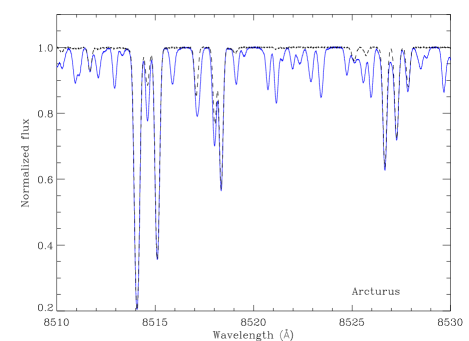
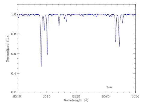
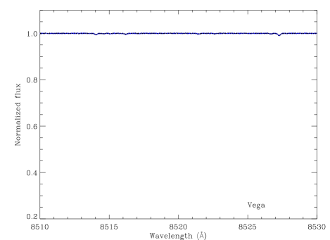
Figure 1: Synthetic spectra used on the atomic line list calibration validation (continuous line). Noise was artificially added to the spectra. The S/N value adopted was 400. The figure also shows the spectra generated only with atomic lines (dotted line).

3.2 Methodology and Definition of CE parameters

The performance function was defined in a way that it compares models (spectra generated by ALiCCE) with simulated observations (input synthetic spectra with noise), wavelength by wavelength pixel. If too many pixels are considered at once, the importance of each pixel to the total performance function becomes increasingly small. If we are aiming to calibrate not only the strong lines, but also the weak ones, we cannot perform the calibration in large wavelength ranges at a time. On the other hand, the calibration cannot be performed in wavelength ranges excessively small because some lines can have widths of several angstroms (sometimes even tenths of angstroms).

Besides, the number of tried solutions ($N$) as well as the number of maximum iterations ($k_{max}$), and consequently the computation time, are directly related with the number of free parameters to be adjusted. This means that if we choose a large wavelength range to perform the calibration at once the problem might become unfeasible.

The calibration can be performed in small steps of wavelengths at a time. The only compromise that must be respected is to choose a wavelength range which is large enough to encompass the entire lines (center and wings) that will be calibrated. For this calibration process we performed the calibration in steps of 1.5 Å width, with an overlap of 0.5 Å width from one to another.

It is also important to mention that although we are calibrating only 1.5 Å  at a time, all the spectra are always generated for a much larger wavelength range (at least 5 Å to each side) to ensure no border effect will be important.

Another constrain that has to be defined is the interval in which each atomic parameter can vary in the first iteration. Errors in the atomic parameters can be as high as 400% (Wiese & Fuhr, 2006), so that was the initial interval chosen for all of them.

For the remaining CE parameters, after many tests we adopted $k_{max}$ = 2000, $\alpha$ = 0.5, $q$ = 6, $N$=1000 and $N_{elite}$ = $0.05N$ for the calibration of each 1.5 Å, which were the most efficient for the performance of the technique.

4 Results

ALiCCE begins the calibration by randomly choosing a value for $\log(gf)$, $\log~{}\Gamma_{StarK}$ and $\log\Gamma_{vdW}$ (within the limits of 400% of the original values) for each line in the given wavelength interval, for each of the 1000 tentative solutions. This will create 1000 different atomic line lists per iteration. For each of these lists, SYNTHE will generate a synthetic spectrum with the atmospheric parameters of the Sun, Arcturus and Vega. These spectra will be compared with the simulated observed spectra and each list will be ranked by their performance function (equation 8). New limits for the atomic parameters will be defined from the top 5% of these lists and the process will be repeated 2000 times. By the end of this process we expect to recover the atomic parameters used to generate the synthetic spectrum with noise for the lines that are present with a reasonable strength in at least one of the stars used in the calibration.

If a line is too weak or not even present in at least one of the stars used in the calibration, we don’t expect to recover its original parameters. Since we used synthetic spectra for this validation test we have prior information about which lines are expected to be recovered by our code. When we produce synthetic spectra with SYNTHE, it generates an output in which it tabulates the contribution of each line in the spectra. The numbers correspond to the per mil residual intensity at line center if the line were computed in isolation. Table 3 shows examples of these values for some of the lines in our interval. The closer the residual intensities are to 1.0, the weaker is the line. Lines weaker than $10^{-4}$ of the continuum will not be present in this output. Lines that appear as 1.0000 are rounded up values.

Table 3: Contribution of some lines in the spectra generated by SYNTHE.

$\lambda$	Element	Arcturus	Sun	Vega	Sum
(nm)		Residual	Residual	Residual
851.3916	ZrI	0.9936	0.9998	1.0000	2.9934
851.4005	FeII	0.9993	0.9978	0.9975	2.9946
851.4072	FeI	0.1365	0.3726	0.9931	1.5022
851.4599	SiI	0.8285	0.7805	0.9972	2.6062
851.4629	TiI	0.9998	1.0000	1.0000	2.9998

As a result of the present test, all lines where the sum in column 6 of table 3 is smaller than 2.800 had their $\log(gf)$ recovered (which means 8 lines in this 20 Å interval - central wavelengths, in nm: 851.4072, 851.4599, 851.5109, 851.7085, 851.8028, 851.8352, 852.6628, 852.7198). For the broadening parameters the lines have to be stronger. The $\log\Gamma_{vdW}$, important in cool stars, was only recovered for very strong lines in Arcturus (Arcturus index in Table 3 smaller than 0.2, which means 2 lines in the 20 Å interval). The $\log\Gamma_{Stark}$ is more important in hot stars, so Vega was important here. Since in the interval chosen there was no strong lines in Vega, $\log\Gamma_{Stark}$ did not converge for any line.

As an example of the convergence behavior, figure 2 shows the $\log(gf)$ recovery for the lines listed in Table 3. In this figure, the blue dotted line shows the expected value of $\log(gf)$, and the black line shows the evolution of the values found by ALiCCE as a function of iteration. The only two lines that converged to the expected value in this figure are lines 851.4072 and 851.4599. However, line 851.3916 converged to a value which is not the nominal value for this line. In this validation test we have this information, but when applying the code for real stars, how will it be possible to distinguish between the correct values and the incorrect converged ones? It is clear that a simple visual inspection of figure 2 is not enough.

The criteria to select between the correct converged values and the incorrect ones are shown in Figure 3. The top figure shows the difference between the average value of $\log(gf)$ found by ALiCCE ($<\log(gf)>$) and the original value used to generate the comparison spectra ($\log(gf_{or})$) as a function of their uncertainties $\sigma_{\log(gf)}$, as defined in Section 2.3. In this figure we show that parameters that converged to their expected values have small uncertainties. These are the lower left points (small $<\log(gf)>$ - $\log(gf_{or})$). Some of these points are actually different points superimposed. It is important to realize that not all points with small $<\log(gf)>$ - $\log(gf_{or})$ converged. Although their average value oscillates around the expected value, they did not converge to this value, and thus, have larger uncertainties. We marked all points values of $<\log(gf)>$ - $\log(gf_{or})<0.005$ in blue.

The bottom figure shows this effect more clearly. In this figure we show the uncertainties in the $\log(gf)$ as a function of the iteration of the convergence, as defined in section 2.3. Blue points are the same as in the top figure. Lines that converged to their expected values do so in the first iterations. Using this as a criteria, we can identify lines that converged to an expected value even if we don’t know this value a priori, or have any knowledge of their contribution in the spectra of the stars. Based on our results we defined that lines that converged to the expected value do so in less than 500 iterations, and have uncertainties smaller than 0.1. These limits are marked by dotted lines in this figure. This is the main reason for the stopping criteria of the method to be the maximum number of iterations ($k_{\mathrm{max}}$), and not a predefined value of convergence. Given these results we believe that ALiCCE is an efficient tool for the calibration of atomic line lists for stellar spectrum synthesis.

Amongst the parameters the code calibrates, $\log(gf)$ was the one with higher success of recovery. This is not surprising as $\log(gf)$ usually is the main parameter (amongst the ones studied) that drives the line profile. For the broadening parameters the recovery rate was much lower. The recovery of the broadening parameters is extremely dependent on the stellar rotational velocity. If the rotational velocity is too high, these parameters cannot be recovered, since the Doppler broadening effect will dominate the line profile. For the velocity of the stars used in these calibrations we can recover the broadening parameter only for very strong lines.

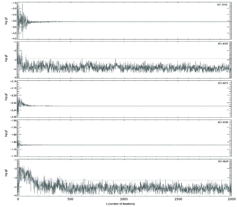
Figure 2: Example of the evolution of the values of log gf found by ALiCCE at each iteration (black line) for the lines in table 3. The doted blue line shows the expected value.

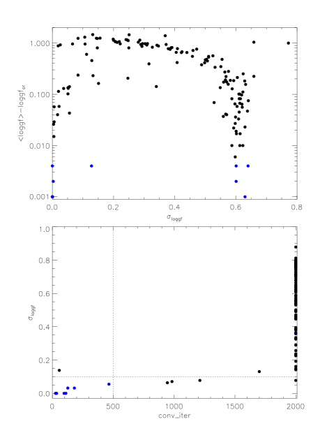
Figure 3: Convergence criteria. The top panel shows the difference between expected values and the values found by ALiCCE for each line in the interval, as a function of the errors calculated for the calibration process. Points where $<\log(gf)>$ - $\log(gf_{or})<0.005$ were marked in blue. The bottom panel shows the errors from the calibration process as a function of the iteration in which the line converged to a single value. Blue points are the same as in the top figure. The dotted lines mark the criteria for convergence: values that converged in less than 500 iterations, and have uncertainties smaller than 0.1. Lines that converged to the expected value are located in the bottom left of this figure.

4.1 Results with observed spectra

We performed a test with real data, applying the method to a small wavelength region from 8517 to 8519 Å. Figures 4 and 5 show the results for the Sun and Arcturus respectively (Vega is almost featureless in this wavelength region, see Fig. 1). The observed solar spectrum was obtained from Kurucz (2005), which is a revised solar flux atlas from Kurucz et al. (1984), and Arcturus spectrum from Hinkle et al. (2000).

This test illustrates the importance of calibrating the line list with more than one star: some of the lines in the synthetic spectra are too weak for one star while too strong for the other. Calibrating these lines for one of the stars alone would induce larger uncertainties in the other. In general, both spectra improved as shown by the values of the $\chi^{2}$ calculated from the difference between observed and synthetic spectra: 10% improvement for Arcturus and 2% for the Sun. The improvement of one line at 8518.028 Å  is particularly obvious. The non-fitted lines at 8517.30 Å  and 8518.45 Å  indicate possible missing lines in the atomic lines list.

A forthcoming paper will focus on the actual calibration of a larger wavelength window using new high-quality observed data, and with the inclusion of several missing lines.

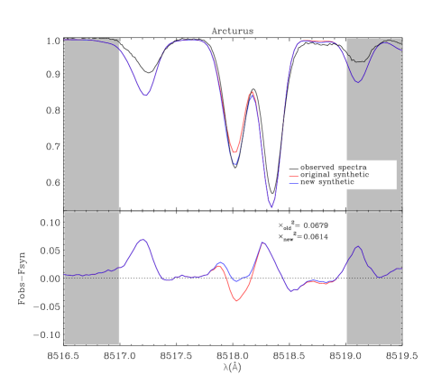
Figure 4: Comparison between the synthetic spectra generated for Arcturus before (red line) and after (blue line) the calibration of the atomic line list by ALiCCE, using a real observed spectrum (black line).

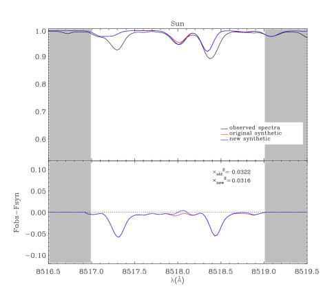
Figure 5: Comparison between the synthetic spectra generated for the Sun before (red line) and after (blue line) the calibration of the atomic line list by ALiCCE, using a real observed spectrum (black line).

4.2 Physical Meaning

Ideally, the calibration of atomic lines through this process could give us insights on atomic physics and structure. This would be true if the physics and numerical approximations adopted in the codes used to model atmospheres and spectra were valid, and if the errors in the stellar atmospheric parameters (temperature, superficial gravity, chemical abundances, etc) were negligible. However, it is known that there are a lot of approximations adopted in the models (e.g. plane-parallel geometry, local thermodynamic equilibrium, convection treatment, etc). This means that when an atomic line in a synthetic spectrum does not fit the observations, many other effects besides their imprecise atomic parameters might be playing a role.

Since we have no way of quantifying exactly how much each of these approximations affect the line profiles, it is inevitable that when we calibrate the atomic line list using a given model atmosphere and a given synthesis code the values found might sometimes compensate for these effects. What comes from this is that the interpretation of the values found in terms of atomic physics might be compromised, and mainly, that the calibrated line list created by ALiCCE should only be used for the same atmosphere models and synthesis codes for which they were calibrated.

5 Conclusion

In this work we present the validation of the ALiCCE code for calibrating atomic line lists used by spectral synthesis codes to generate stellar spectra called ALiCCE, which uses the Cross-Entropy algorithm. For validating our technique we simulated a calibration against synthetic spectra with noise of three well known stars with very well determined atmospheric parameters: the Sun, Arcturus and Vega.

The results obtained show that the Cross-Entropy algorithm is effective to recover the atomic lines parameters used in line lists of spectral synthesis codes for lines with of the continuum flux. The code was able to recover the $\log(gf)$ of the lines that had reasonable signal in at least one of the three stars. In addition, the code is able to recover broadening parameters of very strong lines, when they are present.

It is important to realize that the calibration of the atomic line list is tied to a given model atmosphere and synthesis code. In this version of ALiCCE we used ATLAS9 model atmospheres and SYNTHE spectral code. Any line list calibrated with this version of ALiCCE should only be used for these codes.

References

- Anstee & O’Mara (1995) Anstee S. D., O’Mara B. J., 1995, MNRAS, 276, 859
- Bacławski (2011) Bacławski A., 2011, European Physical Journal D, 61, 327
- Barbuy et al. (2003) Barbuy B., Perrin M.-N., Katz D., Coelho P., Cayrel R., Spite M., Van’t Veer-Menneret C., 2003, A&A, 404, 661
- Barklem et al. (1998) Barklem P. S., Anstee S. D., O’Mara B. J., 1998, PASA, 15, 336
- Barklem & O’Mara (1997) Barklem P. S., O’Mara B. J., 1997, MNRAS, 290, 102
- Barklem et al. (2000) Barklem P. S., Piskunov N., O’Mara B. J., 2000, A&AS, 142, 467
- Bell et al. (1994) Bell R. A., Paltoglou G., Tripicco M. J., 1994, MNRAS, 268, 771
- Blackwell-Whitehead et al. (2008) Blackwell-Whitehead R. J., Pickering J. C., Jones H. R. A., Nilsson H., Hartman H., 2008, Journal of Physics Conference Series, 130, 012002
- Borrero et al. (2003) Borrero J. M., Bellot Rubio L. R., Barklem P. S., del Toro Iniesta J. C., 2003, A&A, 404, 749
- Caproni et al. (2013) Caproni A., Abraham Z., Monteiro H., 2013, MNRAS, 428, 280
- Caproni et al. (2009) Caproni A., Monteiro H., Abraham Z., 2009, MNRAS, 399, 1415
- Caproni et al. (2011) Caproni A., Monteiro H., Abraham Z., Teixeira D. M., Toffoli R. T., 2011, ApJ, 736, 68
- Castelli & Kurucz (1994) Castelli F., Kurucz R. L., 1994, A&A, 281, 817
- Castelli & Kurucz (2004) Castelli F., Kurucz R. L., 2004, A&A, 419, 725
- Civiš et al. (2012) Civiš S., Ferus M., Kubelík P., Jelinek P., Chernov V. E., Zanozina E. M., 2012, A&A, 542, A35
- de Boer et al. (2005) de Boer P. T., Kroese D. P., Mannor S., Rubinstein R. Y., 2005, Annals of Operatons Research, 134, 19
- Den Hartog et al. (2011) Den Hartog E. A., Lawler J. E., Sobeck J. S., Sneden C., Cowan J. J., 2011, ApJS, 194, 35
- Derouich et al. (2003) Derouich M., Sahal-Bréchot S., Barklem P. S., O’Mara B. J., 2003, A&A, 404, 763
- Dimitrijević et al. (2003) Dimitrijević M. S., Ryabchikova T., Popović L. Č., Shulyak D., Tsymbal V., 2003, A&A, 404, 1099
- Fuhr & Wiese (2006) Fuhr J. R., Wiese W. L., 2006, J. Phys. Chem. Ref. Data., 35, 1669
- Gray (1981) Gray D. F., 1981, ApJ, 251, 155
- Hinkle et al. (2000) Hinkle K., Wallace L., Valenti J., Harmer D., 2000, Visible and Near Infrared Atlas of the Arcturus Spectrum 3727-9300 A
- Jorissen (2004) Jorissen A., 2004, Physica Scripta Volume T, 112, 73
- Klose et al. (2002) Klose J. Z., Fuhr J. R., Wiese W. L., 2002, Journal of Physical and Chemical Reference Data, 31, 217
- Konjević et al. (2002) Konjević N., Lesage A., Fuhr J. R., Wiese W. L., 2002, Journal of Physical and Chemical Reference Data, 31, 819
- Kroese et al. (2006) Kroese D. P., Porotsky S., Rubinstein R. Y., 2006, Methodol. Comput. Appl. Probab., 8, 383
- Kurucz (1970) Kurucz R. L., 1970, SAO Special Report, 309
- Kurucz (1992) Kurucz R. L., 1992, RMxAA, 23, 45
- Kurucz (2005) Kurucz R. L., 2005, Memorie della Societa Astronomica Italiana Supplementi, 8, 189
- Kurucz (2011) Kurucz R. L., 2011, Canadian Journal of Physics, 89, 417
- Kurucz & Avrett (1981) Kurucz R. L., Avrett E. H., 1981, SAO Special Report, 391
- Kurucz et al. (1984) Kurucz R. L., Furenlid I., Brault J., Testerman L., 1984, Solar flux atlas from 296 to 1300 nm
- Lesage et al. (1999) Lesage A., Konjevic N., Fuhr J. R., 1999, in Herman R. M., ed., Spectral Line Shapes Vol. 467 of American Institute of Physics Conference Series, Progress in spectral line shapes and shifts evaluation of experimental Stark broadening parameters. pp 27–36
- Margolin (2004) Margolin L., 2004, Annals of Operations Research, 134, 201
- Martins & Coelho (2007) Martins L. P., Coelho P., 2007, MNRAS, 381, 1329
- Meléndez & Barbuy (2009) Meléndez J., Barbuy B., 2009, A&A, 497, 611
- Meléndez et al. (2003) Meléndez J., Barbuy B., Bica E., Zoccali M., Ortolani S., Renzini A., Hill V., 2003, A&A, 411, 417
- Monteiro et al. (2010) Monteiro H., Dias W. S., Caetano T. C., 2010, A&A, 516, A2
- Munari et al. (2005) Munari U., Sordo R., Castelli F., Zwitter T., 2005, A&A, 442, 1127
- Oliveira et al. (2013) Oliveira A. F., Monteiro H., Dias W. S., Caetano T. C., 2013, A&A, 557, A14
- Peterson et al. (2006) Peterson D. M., Hummel C. A., Pauls T. A., Armstrong J. T., Benson J. A., Gilbreath G. C., Hindsley R. B., Hutter D. J., Johnston K. J., Mozurkewich D., Schmitt H. R., 2006, Nature, 440, 896
- Pickering et al. (2011) Pickering J. C., Blackwell-Whitehead R., Thorne A. P., Ruffoni M., Holmes C. E., 2011, Canadian Journal of Physics, 89, 387
- Rubinstein (1997) Rubinstein R. Y., 1997, European Journal of Operational Research, 99, 89
- Rubinstein (1999) Rubinstein R. Y., 1999, Methodology and Computing in Applied Probability, 2, 127
- Ruffoni et al. (2013) Ruffoni M. P., Allende Prieto C., Nave G., Pickering J. C., 2013, ApJ, 779, 17
- Safronova & Safronova (2010) Safronova U. I., Safronova M. S., 2010, Journal of Physics B Atomic Molecular Physics, 43, 074025
- Sbordone et al. (2004) Sbordone L., Bonifacio P., Castelli F., Kurucz R. L., 2004, Memorie della Societa Astronomica Italiana Supplementi, 5, 93
- Shchukina & Vasil’eva (2013) Shchukina N. G., Vasil’eva I. E., 2013, Kinematics and Physics of Celestial Bodies, 29, 53
- Short & Lester (1996) Short C. I., Lester J. B., 1996, ApJ, 469, 898
- Smith (1978) Smith M. A., 1978, ApJ, 224, 584
- Sobeck et al. (2007) Sobeck J. S., Lawler J. E., Sneden C., 2007, ApJ, 667, 1267
- Stalin et al. (1997) Stalin C. S., Trivedi C., Sinha K., Sanwal B. B., 1997, Bulletin of the Astronomical Society of India, 25, 353
- Taklif (1990) Taklif A. G., 1990, Physica Scripta, 42, 69
- Wahlgren (2010) Wahlgren G. M., 2010, in Monier R., Smalley B., Wahlgren G., Stee P., eds, EAS Publications Series Vol. 43 of EAS Publications Series, Oscillator Stengths and Their Uncertainties. pp 91–114
- Wiese & Fuhr (2006) Wiese W. L., Fuhr J. R., 2006, in Weck P. F., Kwong V. H. S., Salama F., eds, NASA LAW 2006 New Critical Compilations of Atomic Transition Probabilities for Neutral and Singly Ionized Carbon, Nitrogen, and Iron. p. 278
- Wiese et al. (2011) Wiese W. L., Fuhr J. R., Bridges J. M., 2011, in 2010 NASA Laboratory Astrophysics Workshop Towards More Accurate Atomic Oscillator Strengths. p. C16
- Wood et al. (2013) Wood M. P., Lawler J. E., Sneden C., Cowan J. J., 2013, ApJS, 208, 27