Extremely Red Quasars from SDSS, BOSS and WISE:
Classification of Optical Spectra

Abstract

Quasars with extremely red infrared-to-optical colours are an interesting population that can test ideas about quasar evolution as well as orientation, obscuration and geometric effects in the so-called AGN unified model. To identify such a population we match the quasar catalogues of the Sloan Digital Sky Survey (SDSS), the Baryon Oscillation Spectroscopic Survey (BOSS) to the Wide-Field Infrared Survey Explorer (WISE) to identify quasars with extremely high infrared-to-optical ratios. We identify 65 objects with $r_{\rm AB}-W4_{\rm Vega}>14$ mag (i.e., $F_{\nu}({\rm 22\mu m})/F_{\nu}(r)\raisebox{-2.58334pt}{$\,\stackrel{{\scriptstyle\raisebox{-0.60275pt}{$\textstyle>$}}}{{\sim}}\,$}1000$). This sample spans a redshift range of $0.28<z<4.36$ and has a bimodal distribution, with peaks at $z\sim 0.8$ and $z\sim 2.5$. It includes three $z>2.6$ objects that are detected in the $W4$-band but not $W1$ or $W2$ (i.e., “W1W2-dropouts”). The SDSS/BOSS spectra show that the majority of the objects are reddened Type 1 quasars, Type 2 quasars (both at low and high redshift) or objects with deep low-ionization broad absorption lines (BALs) that suppress the observed $r$-band flux. In addition, we identify a class of Type 1 permitted broad-emission line objects at $z\simeq 2-3$ which are characterized by emission line rest-frame equivalent widths (REWs) of $\gtrsim$150Å, much larger than those of typical quasars. In particular, 55% (45%) of the non-BAL Type 1s with measurable CIV in our sample have REW(CIV) $>$ 100 (150)Å, compared to only 5.8% (1.3%) for non-BAL quasars in BOSS. These objects often also have unusual line ratios, such as very high N v/Ly$\alpha$ ratios. These large REWs might be caused by suppressed continuum emission analogous to Type 2 quasars; however, there is no obvious mechanism in standard Unified Models to suppress the continuum without also obscuring the broad emission lines.

1 Introduction

Quasars are the most luminous non-transient objects in the Universe, with $L_{\rm bol}$ reaching $\sim$$10^{47-48}$ erg s^-1, powered by accretion of matter onto supermassive black holes. To explain how quasars are fueled and become active, models (e.g., Sanders et al., 1988; Hopkins et al., 2005, 2006) suggest that mergers between gas-rich galaxies produce starbursts and drive gas to the inner galactic nuclear regions. This activity fuels the growth of the supermassive black holes, which actively accrete matter at this stage, with much of the black hole growth happening in this ultra-violet (UV) and optically obscured phase. Feedback, potentially from a radiation-driven quasar wind, leads to removal of gas and dust from the central region, allowing the quasar to be seen in the UV and optical. These major-merger models are invoked to explain the obscuration/reddening observations noted in e.g., Urrutia et al. (2008), Glikman et al. (2012), and predict that red/obscured quasars should appear preferentially during an early stage of quasar evolution. However, the exact nature of the AGN triggering mechanism is not straightforward, as observations find that levels of disturbance in AGN hosts are consistent with those of inactive control samples (e.g. Kocevski et al., 2012; Villforth et al., 2014), or only slightly elevated at low-$z$ (Rosario et al., 2015).

Quasars appear with a wide range of observational properties. Intrinsically luminous quasars may or may not appear bright at optical, ultra-violet and X-ray wavelengths. Much of this variance can be explained in the context of the geometry-based ‘unification models’ (Antonucci, 1993). If gas and dust are present near the active nucleus but do not completely surround it, then some lines of sight to the nucleus are clear, whereas others are blocked. In the former case, the observer can directly view the emission from the accretion disk, with the quasar appearing bright at X-ray, ultra-violet and optical wavelengths; these objects are termed unobscured active galactic nuclei. Often these objects display broad (several thousand ${\rm~{}km~{}s}^{-1}$) emission lines in the optical spectra and are classified as ‘Type 1’ quasars (Khachikian & Weedman, 1974). Less than complete blockage of the quasar continuum by dust will redden the spectrum (e.g., Richards et al., 2003; Krawczyk et al., 2015).

This contrasts with the situation where the observer’s line of sight is blocked by circumnuclear clouds; in this case X-rays are absorbed by the intervening gas and ultra-violet and optical photons are scattered and absorbed by the intervening dust. At optical wavelengths, often the only signature of nuclear activity in this case is strong, narrow emission lines produced in the material illuminated by the quasar along unobscured directions. These objects with weak ultra-violet and optical continua are obscured AGN, and if narrow UV/optical emission lines are present, are designated Type 2 sources (Antonucci & Miller, 1985; Smith et al., 2002; Zakamska et al., 2003; Brandt & Hasinger, 2005; Reyes et al., 2008). Thus, obscuration, as part of an evolutionary phase or an orientation effect, is critical in determining the observed properties of quasars. However, because of their faintness at rest-frame optical and ultra-violet wavelengths, identifying obscured objects, at the peak of quasar activity $z\sim 2$, remains challenging (Stern et al., 2002; Norman et al., 2002; Alexandroff et al., 2013; Greene et al., 2014).

The circumnuclear clouds of gas and dust absorb X-ray, ultra-violet and optical radiation from the quasar and re-emit this energy thermally at infrared wavelengths. This is why unobscured quasars have similar luminosities at near- and mid-infrared wavelengths ($\sim 2-30\mu$m in the rest-frame) as they do in the optical and in the ultra-violet (Elvis et al., 1994; Richards et al., 2006; Polletta et al., 2008; Elvis, 2010). Extremely obscured and dusty objects, in which optical emission is partially extincted or completely blocked, are therefore expected to show much higher infrared-to-optical ratios than unobscured quasars. Indeed, a host of previous studies have used a K-band excess selection (Chiu et al., 2007; Maddox et al., 2008; Jurek et al., 2008; Nakos et al., 2009; Souchay et al., 2009; Wu & Jia, 2010; Peth et al., 2011; Wu et al., 2011; Maddox et al., 2012; Fynbo et al., 2013; Wu et al., 2013), a near-infrared+radio selection (Glikman et al., 2004, 2007; Glikman et al., 2012, 2013) or a mid-infrared selection (Lacy et al., 2004; Stern et al., 2005; Martínez-Sansigre et al., 2006; Richards et al., 2009; Donley et al., 2012; Stern et al., 2012; Banerji et al., 2013; Assef et al., 2013) to identify obscured (as well as unobscured) AGN.

In this paper, we describe a search for quasars with extremely red colours in order to study their range of spectral properties. We use optical photometry and spectroscopy from the Sloan Digital Sky Survey (SDSS; York et al., 2000) and the SDSS-III (Eisenstein et al., 2011) Baryon Oscillation Spectroscopic Survey (BOSS; Dawson et al., 2013) as well as mid-infrared photometry from the Wide-Field Infrared Survey Explorer (WISE; Wright et al., 2010). A companion paper (Hamann et al. 2015, in prep.) presents a detailed investigation into a new class of objects, the extreme rest-frame equivalent width quasars, which are introduced here.

This paper is organized as follows. In Section 2, we describe our datasets and sample selection, and in Section LABEL:sec:key_props we present the basis sample properties of the extremely red quasars. In Section LABEL:sec:spectral_egs we discuss the optical spectra of the extremely red quasars, classifying objects along the traditional lines of broad-line Type 1s, narrow-line Type 2s and those with interesting absorption features. In Section LABEL:sec:erews, we introduce the new class of extreme equivalent width quasars. In Section LABEL:sec:spectral_selection we discuss the selection of the extremely red quasars and place these objects in a broader physical and evolutionary context. We conclude in Section LABEL:sec:conclusions.

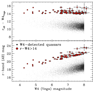
Figure 1: Top: $r-W4$ colour of the $W4$-detected SDSS/BOSS quasars (black dots) as a function of $W4$ (i.e., 22$\mu$m) magnitude. The quasars with $r-W4>14$ are shown as large red circles. Bottom: The $r_{\rm AB}$-band magnitude versus $W4$. As a guide, $W4_{\rm Vega}=8.0$ mag corresponds to $W4_{\rm AB}=14.6$, or a flux density of $F_{\nu}\approx 6$mJy (Wright et al., 2010).

2 Data and Sample Selection

2.1 Parent dataset

Our starting point is the spectroscopic quasar catalogues of the SDSS Seventh Data Release (DR7Q; Schneider et al., 2010; Shen et al., 2011) and the SDSS-III Tenth Data Release (DR10Q; Pâris et al., 2014). SDSS quasar targets with $i\leq 19.1$ were selected if the colours were consistent with being at redshift $z\lesssim 3$, and $i\leq 20.2$ objects were selected if $z\gtrsim$3, as outlined in Richards et al. (2002). BOSS quasar targets are selected to a magnitude limit of $g\leq 22.0$ or $r\leq 21.85$, with the primary goal to select quasars in the redshift range $2.2\leq z\leq 3.5$ as described by Ross et al. (2012, and references therein). In both SDSS and BOSS, quasar targets are also selected if they are matched within 2^′′ (1^′′ in the case of BOSS) of an object in the Faint Images of the Radio Sky at Twenty-cm (FIRST) catalogue of radio sources (Becker et al., 1995). Both the SDSS DR7Q and BOSS DR10Q include quasars that were selected by algorithms other than the main quasar selections; these sources appear in the catalogue due to being targeted by the respective galaxy selections, being a ‘serendipitous’ (Stoughton et al., 2002) or ‘special’ (Adelman-McCarthy et al., 2006) target in SDSS, or an ‘ancillary’ target in BOSS (Dawson et al., 2013; Alam et al., 2015).

Luminous distant quasars are expected to be unresolved in optical ground-based observations, so we use point-spread function (PSF) magnitudes reported in the SDSS DR7 and BOSS DR10 quasar catalogues, corrected for Galactic extinction (Schlegel et al., 1998). Using the 2.5m Sloan telescope (Gunn et al., 2006), imaging data (Gunn et al., 1998) and spectra were obtained with the double-armed SDSS/BOSS spectrographs which have $R=\lambda$/FWHM$\sim$2000 (Smee et al., 2013). Redshifts are measured from the spectra using the methods described in Bolton et al. (2012) and the data products are detailed in the SDSS DR7 (Abazajian et al., 2009) and DR10 (Ahn et al., 2014) papers.

The SDSS DR7 and BOSS DR10 quasar catalogues include 105,783 objects across 9380 deg², and 166,583 objects across 6,370 deg², respectively, with 16,420 objects in common to both catalogues. Thus our superset of optical data has 255,946 objects, and we use the BOSS spectrum (which has higher S/N and a larger wavelength coverage) when there are duplicate spectra between the two catalogues.

WISE mapped the sky in four filters centered at 3.4, 4.6, 12, and 22$\mu$m ($W1$, $W2$, $W3$, and $W4$ bands), achieving $5\sigma$ point-source sensitivities better than 0.08, 0.11, 1, and 6 mJy, respectively. The WISE Explanatory Supplement provides further details about the astrometry and photometry in the source catalogue. We retrieved photometric quantities for each of the four WISE bands. Hereafter, we use the notation SNR_Wx for the signal-to-noise ratio and $Wx$ for the Vega-based WISE magnitudes, in band $x=1,2,3$ and 4.

Because of established conventions, we report Sloan Digital Sky Survey (SDSS) $ugriz$ magnitudes on the AB zero-point system (Oke & Gunn, 1983; Fukugita et al., 1996), while the Wide-Field Infrared Survey Explorer (WISE) $W1-4$ magnitudes are calibrated on the Vega system (Wright et al., 2010). For WISE bands, $m_{\rm AB}=m_{\rm Vega}+\Delta m$ where $\Delta m=(2.699,3.339,5.174,6.620)$ for $W1$, $W2$, $W3$ and $W4$, respectively (Cutri et al., 2011). We make use of the Explanatory Supplement to the WISE All-Sky Data Release, as well as the WISE AllWISE Data Release Products online.

The WISE team has released two all sky catalogues: the 9 month cryogenic phase of the mission led to the WISE All-Sky (“AllSky”) Data Release; while the WISE AllWISE Data Release (“AllWISE”) combines the AllSky data with the NEOWISE program (Mainzer et al., 2011). The resulting AllWISE dataset is deeper in the two shorter WISE-bands ($5\sigma$ point-source sensitivities now 0.054 and 0.071 mJy), and the data processing algorithms were improved in all four $W$-bands. Our analysis began with AllSky, moved to ALLWISE when it became available, but we use both since we had already performed visual inspections using AllSky.

We match the sample of the 255,946 unique quasars in the SDSS DR7Q and BOSS DR10Q, and use both the AllSky and the AllWISE data available at the NASA/IPAC Infrared Science Archive (IRSA), with a matching radius of 2^′′. For the combined DR7Q+DR10Q, we find 203,680 matches; 102,083 objects (96.5%) of the DR7Q and 111,779 (67%) of the DR10Q are matched in one or more WISE bands. The difference in the percentage of matches is expected since BOSS is fainter than SDSS. Matching with DR10Q positions offset in Right Ascension and Declination by 6^′′, 12^′′ and 18^′′ ($\sim$1, 2 and 3 times the WISE angular resolution in W1/2/3) return, respectively, 508, 893 and 873 matches within 2^′′, suggesting our false-positive matching rate is $\lesssim$1% (see also Krawczyk et al., 2013).

With a matching radius of 2$"$, 15,843 of the SDSS DR7 quasars, and 2,979 of the (optically fainter) BOSS DR10 quasars have a good match in the WISE $W4$ band, i.e., SNR${}_{\rm W4}\geq 3$, W4$<8.00$ (close to the nominal 5$\sigma$ point source sensitivity of $W4=7.9$ mags, Wright et al. 2010) and the WISE contamination and confusion flag, cc_flags set to “0000”, suggesting the source is unaffected by known artifacts in all four bands. Table 1 presents an overview of the numbers of SDSS/BOSS quasars in the WISE-matched dataset.

Description	Unique	from	from
	objects	SDSS	BOSS
DR7Q and DR10Q quasarsa	255 946	105 783	166 583
$\quad\shortparallel$ + matched to WISE	203 680	102 083	111 779
$\quad\shortparallel\quad$ + SNR${}_{\rm W4}\geq 3$	52 873	41 922	10 951
$\quad\shortparallel\qquad$ + $W4-\sigma_{W4}\leq 8.00$	28 513	24 041	4 472
$\quad\shortparallel\quad\qquad$ + $W4\leq 8.00$	18 615	16 035	2 580
$\quad\shortparallel\qquad\qquad$ + cc_flags	b17 744	15 300	2 444
and $r-W4>13.0$	286	104	182
and $r-W4>13.5$	136	34	102
and $r-W4>14.0$	65	19	48

Table 1: Overview of the numbers of SDSS/BOSS quasars in the WISE-matched dataset. The third row gives the number of quasars which satisfy $W4$ SNR $\geq 3$; the fourth row is the number of quasars having a magnitude of $W4-\sigma_{W4}\leq 8.00$, while the 5th row is the number having $W4\leq 8.00$. Numbers of objects passing the $r_{\rm AB}-W4_{\rm Vega}$ colour cut is given. ^aThere are objects common to both SDSS DR7Q and BOSS DR10Q that have WISE matches. Hence, the sum of the “From SDSS” and “From BOSS” columns is greater than the given total. ^b“Good” $W4$ detections have SNR${}_{\rm W4}\geq 3$ and $W4<8.00$ and cc_flags equal to “0000”.

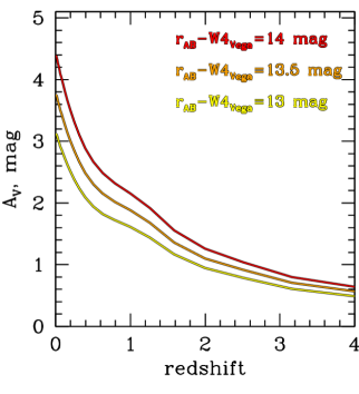
Figure 2: The minimal amount of dust extinction required to produce high infrared-to-optical ratios consistent with our selection criteria, as a function of the redshift of the quasar. The Richards et al. (2006) spectral energy distribution for bright quasars is assumed to represent an unextincted mean quasar. We then apply varying amounts of SMC-like extinction (from Weingartner & Draine, 2001) and convolve with the respective filter curves. We assume $R_{V}\equiv\frac{A_{V}}{E(B-V)}=2.87$ (Gordon & Clayton, 1998). The three curves show the $A_{V}$ values required to generate colours of $r-W4>13$ (yellow) $r-W4>13.5$ (orange) and $r-W4>14$ (red).

2.2 Extremely red quasar criterion

Dey et al. (2008) discovered a population of $z\sim 2$ dust-obscured galaxies, revealed by the Spitzer Space Telescope. In addition to having AGN activity, these objects are strongly star forming and dusty which contributes to their red colours (Brand et al., 2008; Soifer et al., 2008; Pope et al., 2008; Bussmann et al., 2009a, b; Melbourne et al., 2009, 2012). Motivated by this finding, we apply similar selection criteria to the SDSS/BOSS+WISE matched quasars; see Figure 1. At high redshift our WISE $W4$ i.e., 22$\mu$m-based selection, is sensitive to hot dust since $W4$ probes $\lambda\simeq 7.3\mu$m at $z\approx 2$ (Draine & Li, 2007; Elitzur, 2008; Diamond-Stanic & Rieke, 2010). This is of particular interest because at these redshifts shorter wavebands (e.g. $W1$) may cease to trace dust emission, i.e. $W1$ probes $\lambda\simeq 1\mu$m, where dust does not emit strongly.

In particular, we require the spectroscopic quasars to have a reliable detection in the WISE $W4$-band:

$${\rm SNR}_{W4}\geq 3,$$ (1)

a colour of

$$r_{\rm AB}-W4_{\rm Vega}>14.0$$ (2)

i.e., $r_{\rm AB}-W4_{\rm AB}\gtrsim 7.5$, which corresponds to $F_{\nu}({\rm 22\mu m})/F_{\nu}(r)\gtrsim 1000$, and

$$W4_{\rm Vega}\leq 8.00.$$ (3)

We further include objects with $W4>8.00$ if the object has SNR${}_{W4}\geq 3$ and $W4-\sigma_{W4}<8.00$. In Table 1 we outline the stages in the selection and the resulting number of quasars after every step.

The $r-W4>14$ selection has been shown to select Type 2 quasars with $z\sim 2$ (Brand et al., 2006, 2007) and while both Dey et al. (2008) and our selection have a colour cut of $r_{\rm AB}-W4_{\rm Vega}>14.0$, we note that Dey et al. (2008) went to much fainter magnitudes, basing their initial selection in the IR, matched to optical catalogues, and then obtained additional spectra of their candidates. Also, while Dey et al. (2008) start from the IR selection, we start with UV/visible selected quasars in SDSS/BOSS and then look at $W4$ to find the reddest cases.

Our selection applied to both the AllSky and AllWISE catalogues results in very similar samples, and any object that passes the criteria in equations (1)-(3) in either of these data releases is included. There are 65 quasars that have spectra from SDSS/BOSS and satisfy the extremely red criterion from the union between the two WISE datasets.

The $W4$ PSF has a full width at half maximum (FWHM) of 12^′′, much larger than the optical PSF, so a nearby galaxy and a quasar cannot be deblended in $W4$ observations if they are only a few arcseconds apart. To check this possibility, we visually inspected the SDSS and WISE images of the 65 objects using the SDSS Image List Tool and the IRSA WISE Image Service, and found that there is no other obvious optical source (down to the 5$\sigma$-depth of the SDSS photometric survey of $r=22.7$) within 6^′′ of any of our targets. In only two cases there is potential concern that another optical object boosts the $W4$ flux - we return to this in Section LABEL:sec:starburst_egs. We do note, however, that dusty starforming galaxies (particularly at high redshift) are very faint optically, so there is still a possibility that there is an additional contaminating galaxy; inspecting the relatively shallow SDSS images only eliminates the possibility of opitcally bright contaminating galaxies.

Also, although they are bright in $W1$ and $W2$, brown dwarfs tend to be significantly fainter than 8th magnitude in $W4$ (Kirkpatrick et al., 2011), so we do not suspect contamination from these objects. Thus we consider all 65 $r-W4>14$ quasars to be good matches.

2.3 Effects of dust extinction

Before we discuss in detail the observed spectral properties of our sample of extremely red quasars, we describe our expectations for how much extinction would be required to redden the overall spectral energy distribution of a quasar in order for it to be picked up by our colour selection. We acknowledge that the extremely red colours of our objects may not be all due to dust, and thus this exercise is for general guidance.

We simulate the colours of reddened quasars at different redshifts using the Richards et al. (2006) spectral energy distribution of bright quasars, assuming that the spectral energy distributions (SEDs) of all unextincted quasars are the same. We then apply varying amounts of SMC-like extinction (parametrized by the amount of extinction in the V-band, $A_{V}$, in magnitudes), place this object at different redshifts and record its $r-W4$ colour.

The result is shown in Figure 2, where the amount of extinction as a function of redshift is shown to generate colours of $r-W4>13$, $r-W4>13.5$ and $r-W4>14$ (the yellow, orange and red curves, respectively). The amount of extinction is very sensitive to the redshift of the quasar, and here we are only concerned with the dust reddening of a Type 1 SED. If there is any optical emission that is not affected by the circumnuclear dust extinction – for example, the extended emission from the host galaxy – then it would make a reddened quasar appear less red in the $r-W4$ colour. Thus the values of $A_{V}$ plotted in Figure 2 should be regarded as lower limits on the amount of quasar extinction to produce the requisite colours. At low redshifts, the observed $r-$band probes rest-frame optical emission of the quasar, so the amount of extinction necessary to produce a very red optical-to-infrared colour is considerable. However, at high redshifts (where BOSS observations probe the rest-frame ultra-violet emission), an $A_{V}$ of just a few tenths is sufficient to strongly suppress the ultra-violet emission while having a small effect on the infrared; this produces a very red $r-W4$ colour. Vardanyan et al. (2014) discuss the rest 0.25$\mu$m/7.8$\mu$m luminosities and properties of $1.4<z<5$ quasars in the SDSS, and define ‘obscured’ quasars based on $\gtrsim$5 mags of UV extinction; considerably larger than we consider for our extremely red quasars over the same redshift range.

Due to the shallow nature of the WISE $W4$ band, at high redshift, any $W4$-detected galaxy that does not show nuclear activity will have $L_{\rm IR}>10^{12}L_{\odot}$ and star-formation rates $>100M_{\odot}$ yr^-1. Indeed, many of the non-AGN WISE $W4$ detections will have substantially higher infrared luminosities and SFRs.

We have also checked the $R-W4$ colours of galaxies from the Canada-France-Hawaii Telescope Legacy Survey and find that they again have a range of colours, $\sim$ $9<R-W4$ $\lesssim 15$.

The optical colours of our sample are inconsistent with simple dust extinction of a standard quasar SED (e.g. Richards et al., 2003; Krawczyk et al., 2015) and this is a current area of investigation. We discuss possible solutions to this in our companion papers, Hamann et al. (2015, in prep.) and Zakamska et al. (2015, in prep); in particular, contribution from scattered light is a possibility (e.g., Zakamska et al., 2005, 2006) and so is patchy obscuration Veilleux et al. (2013). In particular, we investigate further the nature of the obscuration from the SEDs, which is not consistent with simple reddening from our analysis. As such, we are very hesitant to draw any futher conclusions on dust reddening and $A_{V}$ values in this paper, and leave detailed discussions to Hamann et al. (2015, in prep).

Table 2: The 65 quasars from SDSS and BOSS that have $r-W4>14$, in order of increasing redshift. The r-band AB magnitude is from either Schneider et al. (2010) or Pâris et al. (2014), corrected for Galactic extinction (Schlegel et al., 1998), while the WISE W4 Vega magnitude is from the AllWISE Data Release catalogue. The Radio fluxes are the integrated flux densities ($F_{\rm int}$) measured in mJy at 20cm from the FIRST survey (Becker et al., 1995). The Rest-frame Equivalent Widths (REWs) in Ångstroms are given for Mg ii at $z\leq 1.5$ and C iv for objects at redshift $z>1.5$. The Full-Width, Half-Maximum (FWHM) of the relevant emission line is also quoted. Objects with similar optical spectral properties are grouped together, using the bitwise values described in Table LABEL:tab:ERQ_bitmask, converted here to binary (with a space gap for easier inspection).

Name	R.A.	Decl.	$z$	r-mag	$W4$ mag	$r-W4$	Radio	REWs	FWHM	Notes	Spectral
(SDSS J)	(J2000)	(J2000)		(AB)	(Vega)		flux/mJy	/ Å	/ km s-1		Classification
101034.27+372514.7	152.64283	37.42077	0.282	18.39$\pm$0.03	4.26$\pm$0.02	14.14	-	-	-	Type 1; Strong narrow [OII], starburst	0000 0101
0941000.8+143614.4	145.25339	14.60402	0.384	19.43$\pm$0.02	5.39$\pm$0.04	14.04	7.6	-	-	Type 1; Strong narrow [OII], starburst	0001 0110
105327.92+375804.2	163.36636	37.96786	0.448	19.64$\pm$0.03	5.59$\pm$0.04	14.05	2.8	-	-	Type 1; Weak [OII], strong [NeIII] and [OIII], post-starburst	0001 1010
112657.76+163912.0	171.74069	16.65334	0.464	19.20$\pm$0.02	4.79$\pm$0.03	14.41	2.4	-	-	Type 1; Strong narrow [OIII], post-starburst	0001 1010
102834.03-023659.6	157.14182	-2.61657	0.470	18.90$\pm$0.02	4.80$\pm$0.03	14.10	68.5	-	-	Type 1 based on MgII, blazar candidate	0001 0001
110550.54+112702.0	166.46059	11.45058	0.498	20.65$\pm$0.05	6.17$\pm$0.06	14.48	2.9	-	-	Potential Type 2 candidate, but broad H$\alpha$	0001 0010
092501.78+274607.9	141.25744	27.76888	0.531	19.43$\pm$0.02	4.47$\pm$0.02	14.97	26.7	-	-	Type 2 in Reyes et al. (2008)	0001 0010
091157.55+014327.5	137.98980	1.72432	0.603	21.48$\pm$0.08	6.60$\pm$0.09	14.88	4.6	-	-	Type 2 in Reyes et al. (2008)	0001 0010
225612.16-010508.0	344.05071	-1.08556	0.651	21.53$\pm$0.07	7.16$\pm$0.13	14.37	3.0	27$\pm$8	1870$\pm$730	Type 2 in Reyes et al. (2008)	0001 0010
161558.92+252736.1	243.99552	25.46004	0.676	22.04$\pm$0.09	7.26$\pm$0.09	14.78	4.2	69$\pm$8	918$\pm$174	Type 2	0001 0010
111354.66+124439.0	168.47776	12.74418	0.680	19.86$\pm$0.03	5.20$\pm$0.04	14.66	4.2	-	-	Red Type 1 (broad H$\beta$, strong [OII], Fe II)	0001 0101
124836.10+424259.3	192.15043	42.71650	0.682	21.61$\pm$0.07	7.32$\pm$0.10	14.29	3.4	22$\pm$11	3103$\pm$1138	Type 2	0001 0010
101303.09+072731.9	153.26288	7.45887	0.697	20.99$\pm$0.05	6.91$\pm$0.10	14.08	-	35$\pm$5	1793$\pm$294	Type 2	0000 0010
154215.25+161648.9	235.56354	16.28028	0.714	21.70$\pm$0.06	7.54$\pm$0.10	14.17	1.5	23$\pm$6	1972$\pm$507	Type 2	0001 0010
144642.28+011303.0	221.67618	1.21751	0.726	21.02$\pm$0.05	6.08$\pm$0.05	14.94	5.8	-	-	Type 2 in Reyes et al. (2008)	0001 0010
005009.81-003900.6	12.54091	-0.65017	0.728	20.11$\pm$0.03	5.87$\pm$0.06	14.24	4.4	-	-	Type 2	0001 0010
142240.99+383710.4	215.67083	38.61957	0.758	20.57$\pm$0.03	6.53$\pm$0.05	14.04	9.8	-	-	Type 2 in Reyes et al. (2008)	0001 0010
140744.00+360109.5	211.93333	36.01931	0.783	21.29$\pm$0.05	6.85$\pm$0.07	14.44	5.3	112$\pm$5	(4000)	Type 1 with O[II]	0001 0101
124231.04+023307.0	190.62933	2.55195	0.785	21.16$\pm$0.05	6.81$\pm$0.08	14.35	-	-	-	Red Type 1	0000 0001
091501.71+241812.1	138.75714	24.30336	0.844	20.39$\pm$0.03	4.82$\pm$0.03	15.57	10.1	-	-	Type 1; Very bright in $W4$	0001 0001
152504.74+123401.7	231.26977	12.56715	0.851	21.14$\pm$0.04	6.92$\pm$0.07	14.22	-	43$\pm$3	1984$\pm$167	Type 2	0000 0010
151354.48+145125.2	228.47702	14.85702	0.881	21.00$\pm$0.04	6.37$\pm$0.05	14.63	7.6	20$\pm$2	2212$\pm$209	Type 2	0001 0010
144855.23+213622.0	222.23016	21.60612	0.882	21.70$\pm$0.07	7.72$\pm$0.12	13.98	5.2	101$\pm$17	7868$\pm$1347	Type 2	0001 0010
210712.77+005439.4	316.80322	0.91096	0.924	20.56$\pm$0.03	6.31$\pm$0.06	14.25	0.5	-	-	Type 1, strong FeII, LoBAL MgII absorption	0011 0001
075257.36+351834.6	118.23901	35.30962	0.926	23.23$\pm$0.30	7.57$\pm$0.19	15.66	-	52$\pm$4	2979$\pm$198	Type 1	0000 0001
141702.32+364839.5	214.25969	36.81098	1.004	21.58$\pm$0.06	6.89$\pm$0.06	14.69	7.8	181$\pm$33	21698$\pm$3680	Type 2	0001 0010
142131.51+210719.4	215.38131	21.12207	1.061	21.78$\pm$0.08	7.72$\pm$0.14	14.06	1.0	37$\pm$4	1425$\pm$137	Type 2	0001 0010
092356.70+230030.9	140.98627	23.00860	1.095	22.34$\pm$0.12	7.68$\pm$0.20	14.66	-	30$\pm$8	2112$\pm$410	Type 2, strong O[II]	0000 0110
091103.50+444630.3	137.76458	44.77511	1.302	20.88$\pm$0.06	6.58$\pm$0.06	14.30	-	-	-	Type 1; Strong FeII emission, LoBAL MgII absorption	0010 0001
111004.78+375236.7	167.51994	37.87686	1.308	20.34$\pm$0.04	5.61$\pm$0.04	14.74	7.1	-	-	Red Type 1	0001 0001
165258.51+390249.7	253.24380	39.04716	1.308	21.21$\pm$0.04	6.79$\pm$0.06	14.42	249.3	7$\pm$1	2966$\pm$304	Type 1 based on MgII, blazar candidate	0001 0001
102425.41+033239.8	156.10589	3.54441	1.477	22.40$\pm$0.17	7.11$\pm$0.17	15.29	-	35$\pm$8	1166$\pm$377	Type 2 based on v. narrow CIV	0000 0010
144929.61+394824.2	222.37341	39.80674	1.491	21.74$\pm$0.06	7.66$\pm$0.11	14.08	24.3	57$\pm$9	10075$\pm$1405	Type 2 based on v. narrow CIV and HeII	0001 0010
153542.41+090341.1	233.92671	9.06143	1.533	21.33$\pm$0.04	6.65$\pm$0.07	14.68	8.1	137$\pm$14	1556$\pm$140	Type 1; Very strong FeII emission in UV2/3, UV1,	0011 0001
										and strong AlIII with weak/absent CIII] and SiIII]; see Appendix LABEL:sec:J1535.
080304.76+532627.0	120.76987	53.44084	1.573	20.85$\pm$0.05	6.60$\pm$0.07	14.26	2.9	123$\pm$7	3196$\pm$138	Type 1; LoBAL	0011 0001
122453.20+084303.2	186.22167	8.71757	1.960	23.55$\pm$0.73	8.01$\pm$0.25	15.54	-	0$\pm$0	0$\pm$0	Red Type 1	0000 0001
211329.61+001841.7	318.37340	0.31161	1.996	23.40$\pm$0.28	8.14$\pm$0.29	15.26	-	192$\pm$7	1536$\pm$49	Type 2, “Extreme” REW (EREW)	1000 0010
163313.29+401338.9	248.30541	40.22749	2.010	21.18$\pm$0.05	7.12$\pm$0.08	14.07	10.5	20$\pm$10	11936$\pm$99	Type 1; Blazar candidate	0001 0001
173049.10+585059.5	262.70459	58.84988	2.035	21.39$\pm$0.07	7.37$\pm$0.09	14.02	-	-	-	Type 1; FeLoBAL	0010 0001
133611.79+404522.9	204.04913	40.75637	2.071	21.07$\pm$0.06	6.38$\pm$0.05	14.69	3.1	20$\pm$3	6244$\pm$688	Type 1	0001 0001
013435.66-093102.9	23.64861	-9.51748	2.220	21.30$\pm$0.06	6.58$\pm$0.07	14.71	960	-	-	Gravitational Lens, Red Type 1, see Appendix LABEL:sec:J0134	0001 0001
084447.66+462338.7	131.19862	46.39411	2.224	21.48$\pm$0.08	7.48$\pm$0.13	14.00	-	175$\pm$4	1744$\pm$34	Type 2, with narrow CIV	0000 0010
094317.59+541705.1	145.82333	54.28475	2.230	21.41$\pm$0.07	7.33$\pm$0.09	14.08	2.2	-	-	Type 1; FeLoBAL	0011 0001
222646.53+005211.2	336.69390	0.86980	2.247	21.54$\pm$0.07	7.54$\pm$0.15	14.00	653	65$\pm$4	2663$\pm$212	Red Type 1, strong associated absorbtion	0001 0001
000610.67+121501.2	1.54449	12.25035	2.309	22.18$\pm$0.13	6.56$\pm$0.07	15.61	-	108$\pm$6	4589$\pm$202	Type 1, EREW	1000 0001
232326.17-010033.1	350.85906	-1.00920	2.355	21.83$\pm$0.08	7.76$\pm$0.22	14.07	-	256$\pm$5	3977$\pm$62	Type 1, N v/Ly$\alpha$ $>1$, EREW	1000 0001
123241.73+091209.3	188.17391	9.20261	2.385	21.09$\pm$0.05	6.78$\pm$0.09	14.31	-	230$\pm$3	4873$\pm$53	Type 1, N v/Ly$\alpha$ $>1$, EREW	1000 0001
083413.90+511214.6	128.55793	51.20407	2.391	19.77$\pm$0.04	5.43$\pm$0.04	14.33	1.9	-	-	Type 1, red slope, $z$ from absorption at red end	0001 0001
0832000.2+1615000.3	128.00085	16.25011	2.423	21.82$\pm$0.08	7.51$\pm$0.16	14.31	1.1	-	-	Type 1, EREW, strong associated absorption lines	1001 0001
011110.83+204543.8	17.79517	20.76218	2.432	22.03$\pm$0.09	7.96$\pm$0.21	14.06	-	0$\pm$0	0$\pm$0	Type 1; Ly-$\alpha$ emitter QSO	0000 0001
090630.73+082837.3	136.62806	8.47705	2.437	21.77$\pm$0.09	7.76$\pm$0.20	14.00	22.8	3$\pm$1	340$\pm$159	Type 1 (from Ly-$\alpha$ width)	0001 0001
093638.41+101930.3	144.16006	10.32510	2.458	21.72$\pm$0.06	7.61$\pm$0.17	14.11	-	169$\pm$4	1273$\pm$20	Type 2, but with EREW	1000 0010
134026.99+083427.2	205.11248	8.57424	2.490	22.31$\pm$0.13	8.10$\pm$0.21	14.21	-	338$\pm$11	2088$\pm$51	Type 2, but with EREW	1000 0010
221524.00-005643.8	333.85003	-0.94550	2.493	22.29$\pm$0.12	7.91$\pm$0.24	14.38	-	152$\pm$5	4226$\pm$112	Type 1; EREW	1000 0001
111017.13+193012.5	167.57139	19.50347	2.497	20.61$\pm$0.03	6.59$\pm$0.07	14.01	-	-	-	Type 1; EREW	1000 0010
155102.79+084401.1	237.76163	8.73366	2.520	20.66$\pm$0.03	6.61$\pm$0.06	14.05	2.9	10$\pm$3	2467$\pm$426	Type 1; FeLoBAL	0011 0001
083448.48+015921.1	128.70202	1.98921	2.594	21.19$\pm$0.05	6.88$\pm$0.09	14.31	-	214$\pm$7	2864$\pm$73	EREW, Type 1	1000 0001
220337.79+121955.3	330.90749	12.33204	2.626	21.57$\pm$0.05	7.45$\pm$0.14	14.12	-	262$\pm$3	1072$\pm$10	EREW, Type 2	1000 0010
085124.78+314855.7	132.85329	31.81548	2.638	21.63$\pm$0.07	6.79$\pm$0.08	14.84	-	76$\pm$5	3584$\pm$181	Type 1, W1W2-dropout	0100 0001
100424.88+122922.2	151.10370	12.48952	2.640	22.15$\pm$0.12	7.87$\pm$0.19	14.28	12.3	-	-	Tpye FeLoBAL	0011 0001
104611.50+024351.6	161.54796	2.73103	2.772	21.51$\pm$0.07	7.11$\pm$0.11	14.40	-	203$\pm$7	5181$\pm$144	Type 1, N v/Ly$\alpha$ $>1$, EREW	1000 0001
155434.17+110950.6	238.64238	11.16407	2.936	21.19$\pm$0.05	6.63$\pm$0.08	14.56	-	-	-	Type 1, BAL, probably FeLoBAL	0010 0001
135959.73+052512.3	209.99888	5.42008	3.055	22.08$\pm$0.11	7.27$\pm$0.09	14.81	-	70$\pm$10	7250$\pm$833	Type 1, W1W2-dropout	0100 0001
022052.11+013711.1	35.21715	1.61976	3.138	21.82$\pm$0.08	7.08$\pm$0.09	14.74	-	341$\pm$19	2843$\pm$167	EREW, Type 1, W1W2-dropout	0100 0001
101439.51+413830.6	153.66466	41.64183	4.360	21.84$\pm$0.08	7.74$\pm$0.16	14.10	-	118$\pm$8	13568$\pm$684	Type 1, (Fe)LoBAL	0010 0001

3 Key Properties of the Extremely Red Quasars

3.1 Magnitudes and redshift distribution

The key properties of the extremely red quasar sample are provided in Table 2: the catalogue name of the object, its Right Ascension, Declination, redshift, and magnitude and colour properties. The Radio fluxes are the integrated flux densities ($F_{\rm int}$) measured in mJy at 20cm from the FIRST survey (Becker et al., 1995). The Rest-frame Equivalent Widths (REWs) are given for Mg ii at $z\leq 1.5$ and C iv for objects at redshift $z>1.5$. The Full-Width, Half-Maximum (FWHM) of the relevant emission line is also quoted, with the REW and FWHM measurements coming from fits to the line profiles, as described in Hamann et al. (in prep.).

General	Bitwise	Number in
Description	Value	Sample
Type 1 Quasar	0000 0001	37
Type 2 Quasar	0000 0010	28
Starburst	0000 0100	5
post-starburst	0000 1000	2
Radio Detected	0001 0000	37
(Fe)LoBAL	0010 0000	10
W1W2-dropouts	0100 0000	3
“Extreme” REWs	1000 0000	12

We give each object a classification based on optical spectral properties, indicated by the bitwise values described in Table LABEL:tab:ERQ_bitmask. These classifications were all performed by visual inspection, with objects assigned to the classes given in Table LABEL:tab:ERQ_bitmask depending on the presence (or absence) of broad/narrow emission lines, broad absorption features, indications of ongoing or recently ceased star-formation, or objects with large equivalent width in the C iv emission line. These visual inspections are generally qualitative but as discussed in Section 4, aid us to understand the sample and physical types of quasars that the $r-W4>14$ colour selects. We also present a short note on each object in Table 2, qualitative assessments based on visual inspection of the optical spectra, and use these notes to make the link between the classifications given in Table LABEL:tab:ERQ_bitmask and the discussions presented in Section LABEL:sec:spectral_egs. We call a quasar “red” when its spectral slope is shallower than the Vanden Berk et al. (2001) template. The acronym EREW stands for Extreme Rest-frame Equivalent Width, referring to a group of objects we introduce and describe in Section LABEL:sec:erews.

The redshift range for the extremely red quasars is $0.282<z<4.36$, and half the sample is fainter than $r$=21.4. Figure LABEL:fig:ERQ_Nofz shows the redshift distribution of the sample compared to the full redshift distribution of the 17,744 SDSS/BOSS quasars with good W4 matches. The redshift distribution of the $r-W4>14$ sample is bimodal, with peaks around $z\sim 0.8$ and $z\sim 2.5$. This bimodality is the result of the two different SDSS quasar selections. The $z\sim 2.5$ redshift peak is due to the increased depth of the BOSS selection, as seen in Figure LABEL:fig:redshift_vs_iband.

In the left panel of Figure LABEL:fig:redshift_vs_iband the redshifts and $i$-band magnitudes are displayed for the $r-W4>14$ objects, and compared to the distributions from the full SDSS DR7 and BOSS DR10 quasar catalogues. SDSS quasars use the $i$-band for selection limits, thus one can identify the $i=19.1$ magnitude limit contour for the SDSS $z\lesssim 2.5$ quasars, as well as the redshift histogram peaks at $z\sim 0.6-1.0$ and $z\sim 2.2-2.7$ seen in the BOSS quasar distribution (e.g. Fig. 2 in Pâris et al., 2014). In the right panel of Fig. LABEL:fig:redshift_vs_iband, the extremely red quasars are compared to the SDSS/BOSS+WISE catalogue, for the fully matched (i.e. any WISE band) sample given by the black contours, and for the $W4$-matched objects only, given by the orange contours. The redshift-$i$ magnitude distribution of the $\approx$18,000 objects with good $W4$ matches is given by the orange contours and points. These $W4$ objects are at the bright end in the optical, and are generally at $z<2$.

Since we are selecting such extreme objects it is important to see how the selection affects the redshift distribution. In Figure LABEL:fig:N_vs_color we show how the number of objects selected, and the sample redshift, depend on $r-W4$ colour. The dip in mean redshift at $r-W4\sim 10-11$ comes from the fact that fainter BOSS quasars, generally at $z\gtrsim 2$, are lost quicker than $z\lesssim 1$ quasars. The upturn at $r-W4>11.5$ is due to the fact that the $W4$-bright BOSS quasars that are very red remain in the sample even to the reddest colours.

Figure LABEL:fig:ERQs_magredshift presents the magnitude-redshift and colour-redshift relations for the SDSS/BOSS+WISE matched catalogue highlighting the extremely red sample. This plot can be directly compared with Yan et al. (2013) (and their Figure 20). Yan et al. (2013) have also merged the WISE photometry with the SDSS (though not BOSS), and describe the spectroscopic observations of eight objects that have $r-W4>14$ (see their Table 1 for details). Although we have an order of magnitude more $r-W4>14$ objects at $z>2$, the Yan et al. objects are significantly fainter in the optical than our SDSS/BOSS detected objects. Based on the spectral properties of the Yan et al. (2013) sample, 3 (out of 8) objects are classified as Type-1 AGN, 3 objects are Type-2 AGN, and the remaining two objects have features consistent with either a Type-2 AGN, or a star-forming galaxy, broadly in line with the composition given in Table LABEL:tab:ERQ_bitmask. Interestingly, Yan et al. (2013) motivate the use of the $r-W4>14$ colour selection in order to select ultraluminous infrared galaxy (ULIRG) candidates, not red quasars (they use the shorter WISE bands to select reddened quasars), and indeed find this colour selection identifies IR luminous galaxies over a wide range of redshift, $z\sim 0.7-3$. However, the relative contribution to the $W4$ luminosity from AGN and star formation warrants investigation, especially at high redshift where the rest-frame 22$\mu$m can probe warm (AGN) dust, as well as PAH features.

3.2 Mid-Infrared Colours of the ERQs

The mid-infrared colour-colour distributions for the SDSS/BOSS quasars that are detected in WISE are shown in Figure LABEL:fig:colorcolor_W1W2W3. Contours are given for the full “good” $W4$ sample, with objects that have redshifts $z<2$ and $z>2$ given by the blue and red contours, respectively. The colours of the extremely red quasar sample are given by the large solid circles. We also split the extremely red quasar sample into three broad classes, ‘Type 1’ (section LABEL:sec:Type1_egs), ‘Type 2’ (sections LABEL:sec:Type2_loz_egs and LABEL:sec:Type2_hiz_egs) and the Extreme Rest-frame Equivalent Width (EREW) objects (section LABEL:sec:erews).

Fig. LABEL:fig:colorcolor_W1W2W3 shows that the Type 2 and EREW quasar populations are redder in $(W2-W3)$ than the general $W4$-detected population. Upon visual inspection of the $W4$-detected objects with very red, $(W2-W3)\gtrsim 3.8$ colours, many were found to lie along the Ecliptic and did not have secure $W4$ photometry due to Mars, Jupiter and Saturn producing a significant number of spurious mid-infrared detections. These detections are not plotted in Fig. LABEL:fig:colorcolor_W1W2W3 and does not affect any of our $r-W4>14$ extremely red quasars.

In $(W1-W2)$, the extremely red quasar population is perhaps slightly more representative of the $W4$-detected population; none of the red quasars are bluer than $(W1-W2)\approx 0.5$. The $W1W2W3$ colour-colour diagram has become a key diagnostic for WISE objects, and its power in separating different classes of objects is seen in Wright et al. (2010); Eisenhardt et al. (2012) and Yan et al. (2013). In particular, Eisenhardt et al. (2012) use a colour selection based on $W1W2W3$ colours to select “W1W2-dropouts”. Three of our quasars satisfy this criterion, signified by the stars in Fig LABEL:fig:colorcolor_W1W2W3. We discuss these objects in Section LABEL:sec:w1w2_drops.

3.3 Radio Properties

Table 2 also gives the radio fluxes of the $r_{\rm AB}-W4_{\rm Vega}>14$ sample. 37 (56%) of the full extremely red quasar sample is detected in the FIRST survey (Becker et al., 1995), which has a flux limit of $\approx$1 mJy at 20 cm, with 22 out of 28 objects at $z<1.1$ (79%) being detected. The magnitude of radio flux at 20cm ranges from 0.55 to 960 mJy.

While the radio loudness is typically defined by the ratio of the 5 GHz radio to 4400Å flux densities (e.g., Kellermann et al., 1989; Padovani et al., 2003), with the advent of the FIRST and SDSS surveys, much of the recent analysis of radio loudness has been done in terms of the 20cm to $i$-band ratio, $\mathcal{R}=f_{\rm radio}/f_{\rm optical}$, e.g., Ivezić et al. (2002), White et al. (2007) and Kratzer & Richards (2015). Typically no $k$-correction is applied as the mean spectral index in the radio and optical are similar (though this assumption may not hold true for these extremely red, and unusual objects). While there is no true gap in the distribution of $\mathcal{R}$, at $\mathcal{R}$$\sim$10 there is a subtle change in the distribution (e.g., White et al., 2007; Kratzer & Richards, 2015) and it is common to refer to objects with $\mathcal{R}\geq 10$ as “radio-loud”. The value of $\mathcal{R}$ can be calculated straight from Table 2 for each of our objects, and we find that all 37 of our radio-detected objects are nominally radio-loud. However, without knowing the extent of reddening from dust in our sources, these values should be considered as an upper limit to the true value of $\mathcal{R}$. We also find that all of the 37 radio-detected objects are unresolved in FIRST.

A total of 30 objects (46%) in our sample have a radio target selection flag set indicating that these objects were detected in the FIRST survey and passed the SDSS/BOSS quasar selection to be observed as quasar targets. Of these 30 objects, 10 are from SDSS and 20 from BOSS. 17 objects (26%) are selected for spectroscopy solely due to their radio properties, all of which are from BOSS.

Yan et al. (2013) discovered ULIRGs at $z\sim 2$ with extremely red colours, which suggests that star-formation will lead to an enhancement of the $W4$ emission we detect from our sample. While the sample definition of $r-W4>14$ selects quasars that are red due to dust obscuration (i.e., the targeted obscured quasar population), there is the possibility it will also select systems with particularly bright IR emission due to star formation. The large fraction of radio-detected quasars in the resulting sample, and the known relations between radio and IR emission from star formation, suggest that this may be an aspect of the extremely red quasar selection.

To investigate this further, we calculate rest-frame 1.4 GHz radio luminosity from the observed fluxes using a radio spectral index of $\alpha=-0.7$. In the first instance, we assume that all of the radio emission is due to star formation, which will result in upper limits on the SFR derived from the radio and MIR. We use the conversions between radio and star formation rates reported in Bell (2003) to calculate the necessary SFRs and total IR luminosity of star formation $L_{\rm SFR,\ 8-1000\mu m}$. Then we scale seven star-formation templates from Kirkpatrick et al. (2012) and Mullaney et al. (2011) to match the SFRs necessary to explain the observed radio emission. We then redshift them to the redshift of the target, convolved with the $W4$ filter from Jarrett et al. (2011) and calculate the predicted IR flux. Figure LABEL:fig:qir shows the ratio between the observed and the predicted $W4$ fluxes; those are shown as black points, where the error bars reflect the spread amongst templates (and therefore provide a measure of the systematic error). For objects undetected in the radio, we can only calculate an upper limit on the SFR rate and thus a lower limit on the observed-to-predicted flux ratio; those are shown as red upward arrows, and those are conservative (i.e., the lowest lower limit of the seven templates). A ratio of $>1$ means the MIR emission is likely AGN dominated, while ratios $<1$ mean the predicted SFR is less than expected, given the radio flux.

There are 37 objects detected in the radio; if all the radio flux is associated with star-formation, which is unlikely, then for these objects the median luminosity due to star formation would need to be $L_{\rm 8-1000\mu m}=10^{13.6}L_{\odot}$ in order to explain the median radio luminosity of $\nu L_{\nu}[{\rm 1.4GHz}]=10^{41.6}$ erg sec^-1. In other words, these objects would need to be forming stars at the median rate of $\approx$7700 $M_{\odot}$ yr^-1 in order to explain the observed radio emission, and this rate is $\sim$4-10$\times$ higher than the e.g. 850$\mu$m-selected submillimeter galaxy (SMG) population at redshifts $z\sim 2-3$ (Wardlow et al., 2013; Fu et al., 2013; Casey et al., 2014). However, this SFR is an upper limit, as the AGN is almost certainly contributing significant flux in all objects. It is more likely that both the radio emission and the $W4$ emission in these objects are due to the AGN and star formation, and thus the SFRs are more in-line with those of SMGs and WISE-selected luminous infrared galaxies (Wu et al., 2012; Jones et al., 2014, 2015; Tsai et al., 2015).

The two points with the lowest $W4_{\rm obs}/W4_{\rm SFR,predicted}$ ratios are potentially beamed sources with an apparent extremely high radio luminosity $\nu L_{\nu}[{\rm 1.4GHz}]\simeq 10^{44.5}$ erg s^-1 which has nothing to do with star formation in the host galaxy (though our data are insufficient to determine the origin of the $W4$ emission in these sources). For the less extreme sources at $z<1$, we find that the required median SFR necessary to explain the observed radio and W4 emission is 2180 $M_{\odot}$ yr^-1, which is still very high, but could potentially be the result of an e.g. (major) merger. While we do not have direct observations (e.g., far-infrared) which would rule out such star formation rates, various authors find it unlikely that star formation dominates mid-infrared and radio emission of luminous Type 2 quasars at $z<1$ (e.g., Harrison et al., 2014; Zakamska & Greene, 2014; Zakamska et al., 2015, in prep.).

The remaining objects are undetected in the radio and therefore we can place only upper limits on star formation rates. For this population we find the median lower limit $W4_{\rm obs}/W4_{\rm SFR,predicted}$ of 2.4, meaning that the star formation is inadequate by at least this factor in explaining the observed W4 flux. Thus we conclude that the $W4$ fluxes in these objects must be dominated by the AGN as well. However, it seems that ultimately, we currently do not have enough data to determine whether the radio emisson is due to AGN or star formation. New FIR/submm data is required, with further SED decomposition, and indeed this is where future analysis will be concentrated (Hamann et al., 2015, in prep.; Zakamska et al., 2015, in prep.).

4 Classifications from optical Spectroscopy

The spectra of the extremely red quasar sample are publicly available at the SDSS-III Science Archive Server. We broadly classify the objects that satisfy the $r-W4>14$ selection into: (i): unobscured (but reddened) Type 1 quasars possessing broad lines (bitwise value 1 in Table 3); (ii): objects that show evidence for being narrow-line Type 2 quasars from their optical spectra (bitwise value 2 in Table 3); (iii): objects that suggest ongoing, or recently ceased star formation (bitwise values 4 and 8); (iv): radio-detected quasars (in the FIRST survey, bitwise value 16); (v): quasars with blue-shifted absorption features (bitwise value 32); (vi): objects that are not detected in the WISE $W1/2$-bands (bitwise 64) and (vii): a class of Type 1 sources with extreme rest equivalent widths in their UV broad lines, namely, REW$>150$Å in either C iv or Mg ii (bitwise 128). These classification groups are not mutually exclusive; several objects are assigned to multiple groups. However, we class all of the sources as either Type 1 (37/65; 57%) or Type 2 (28/65; 43%). These sources are indicated by the bitwise values in the last column of Table 2 and are described in Table LABEL:tab:ERQ_bitmask. Example spectra are presented in what follows.

4.1 Type 1 Quasars

Figure LABEL:fig:Type1_egs presents the spectra of six examples of extremely red quasars, classified as Type 1 based on broad emission lines seen in their optical spectroscopy. Where measured, the mean line widths are FWHM(Mg ii) $\sim 6440$ km s^-1 and FWHM(C iv) $\sim 4900$ km s^-1. Figure LABEL:fig:Type1_egs lists the SDSS name, redshift, classification (from Table LABEL:tab:ERQ_bitmask) and $r-W4$ colour of each object.

The spectra in Figure LABEL:fig:Type1_egs are heterogeneous; some show blue continua, while some are red. The first object (with the lowest redshift in our sample) has unusually broad [O iii] with non-Gaussian structure (Liu et al., 2010, see also section LABEL:sec:starburst_egs). Many of the examples of Type 1 quasars from our selection appear to be significantly reddened (Richards et al., 2003) often with a host galaxy component.

Glikman et al. (2013) identify dust-reddened quasars by matching the FIRST radio catalogue to the UKIRT Infrared Deep Sky Survey (UKIDSS; Lawrence et al., 2007). This study identified 14 reddened quasars with $E(B-V)>0.1$, including three at $z>2$. However, Glikman et al. (2013) find no heavily reddened $(E(B-V)\gtrsim 0.5)$ quasars at high redshifts $(z>2)$. The object ULASJ1234+0907 $(z=2.503)$ discovered by Banerji et al. (2014) is currently the reddest broad-line Type 1 quasar known, with $(i-K)_{\rm AB}>7.1$. Since all our extremely red quasars have $i\lesssim 22$ mag and a range of $1.62<(i-K)_{\rm AB}<4.73$, none of our objects have optical-to-near infrared colours as red as ULASJ1234+0907.

We note the object J165258+390249 has a relatively blue continuum and is clearly not suffering from dust obscuration. This object may be optically variable, and at the time of the optical and IR photometry had a large enough $r-W4$ to satisfy our colour cut. We also note it is a radio source, and has features consistent with an optical blazar spectrum. This further highlights the importance of understanding the radio properties (and potentially the synchrotron radiation contribution) of these quasars and how it affects the IR and the resulting sample of objects.

4.2 Type 2 Quasar candidates at low redshift

We define Type 2 quasars as objects with narrow permitted emission lines that do not have an underlying broad component, and with line ratios characteristic of non-stellar ionizing radiation (Zakamska et al., 2003; Reyes et al., 2008). Specifically, in Type 2 quasars the broad-line region is completely blocked from the observer by strong obscuration ($A_{V}>10$), and nuclear activity is inferred indirectly via the emission line ratios of ionized gas which are characteristic of photo-ionization by the quasar (Baldwin et al., 1981; Veilleux & Osterbrock, 1987). At low redshifts, where H$\beta$ and [O iii] are accessible in the optical spectrum, we can define Type 2 objects as those in which the kinematic structure of the permitted emission lines is similar to that of the forbidden lines; the permitted lines should not display an additional broad (FWHM$\ga 2000$ km sec^-1) component. We also require [O iii] /H$\beta>3$.

Figure LABEL:fig:Type2_loz_egs presents examples of Type 2 quasar candidates at $z\lesssim 1$. No line-fitting has been performed, but all objects in this class are seen by visual inspection to have similar same kinematics in the permitted H$\beta$ and forbidden [O iii] lines. In the extremely red quasar sample, the quasar nature of the Type 2 candidates is not in doubt: the typical values of [O iii] /H$\beta$ are 10 or greater, and high-ionization species such as [NeV] are detected in most cases. However, H$\beta$ can be weak and there may be broad components in some H$\alpha$ lines (Zakamska et al. in prep) which are redshifted out of the BOSS wavelength coverage.

Just over half (60%) of our Type 2s are at $z<1$. This is due to the fact that we are using the spectroscopic quasar catalogues as our initial sample, before matching to the WISE photometry. Thus, from the requirement of having a relatively bright detection in the optical (cf. the Brand et al. studies) there will be a selection bias towards lower redshift objects.

Among the 28 objects with $z<1.1$, 20 (71%) are classified as Type 2 candidates from their optical spectra; see Figure LABEL:fig:Type2_loz_egs. This high fraction of Type 2 objects is completely uncharacteristic of the parent sample of the SDSS/BOSS quasars, making it clear that the selection based on high infrared-to-optical colours can indeed recover obscured quasars. All seven Type 2 quasars in our sample that were observed before July 2006 are found in the catalogue of Reyes et al. (2008).

4.3 Type 2 Quasar candidates at high redshift

We find objects that have narrow emission lines, weak continua and satisfy the definition of Type 2 candidates, at high redshift ($z>1.5$) as well; see Figure LABEL:fig:Type2_hiz_egs. The classifications are performed by visual inspection of the optical spectra and all objects in this class with $z>1.5$ have FWHM(C iv) $\lesssim 2000$ km s^-1.

These objects have similar optical spectra to those described in Yan et al. (2013) and Alexandroff et al. (2013), although there are no objects in common between our sample and that presented in Alexandroff et al. (2013). Those authors present a sample of 145 candidate Type 2 quasars from BOSS at redshifts between 2 and 4.3, using data from DR9 (Ahn et al., 2012). These objects are characterized by weak continuum in the rest-frame ultraviolet with a typical continuum magnitude of $i\approx 22$ (i.e., $M_{i}(z=2.5)\approx-25$) and strong lines of C iv and Ly$\alpha$, with FWHM $\leq 2000{\rm~{}km~{}s}^{-1}$. Typical ($\sim L^{*}$) galaxies are $\geq 1$ magnitude fainter at these redshifts (Marchesini et al., 2007; Marchesini et al., 2012), suggesting host-galaxy light is not sufficient to explain the continuum luminosity and some level of AGN light is getting through/around the absorber.

The reddest quasar in Alexandroff et al. (2013) has $r-W4=13.30$. In general, our selection of Type 2 candidates is not as strict as that of Alexandroff et al. (2013), and we find no overlap between the sample here and the DR9-based sample in Alexandroff et al. (2013). While this class of object shows only narrow emission lines in the rest-frame UV spectra, Greene et al. (2014) obtained near-infrared spectroscopy for a subset of the Alexandroff et al. (2013) sample, demonstrating that the H$\alpha$ emission line consistently requires a broad component. This result implies that the typical extinction in these objects is $A_{V}\lesssim$ a few, sufficient to block the rest-frame UV continuum and broad lines but not the rest-frame optical - consistent with the (relatively) bright continuum.

4.4 Objects with starburst and post-starburst signatures

Our sample includes quasars that have starburst or post-starburst signatures in their optical spectra. Examples are given in Figure LABEL:fig:starburst_egs.

The [OII]/[OIII] ratio can be used as a starburst indicator in AGN and galaxies (e.g., Kauffmann et al., 2003; Groves et al., 2006). Objects from our sample are placed into the starburst class if they exhibit evidence of obvious [O ii] emission (Kennicutt, 1998; Kewley & Dopita, 2002; Kewley et al., 2004; Ho, 2005; Moustakas et al., 2006; Mostek et al., 2012), though we acknowledge that [OII] emission can also be associated with the narrow-line region of the AGN.

The post-starburst objects are objects which have either a Balmer break, and/or an obvious Balmer series, originating from an A-star population that is not dominated by blue light from OB-stellar populations. Quasars with post-starbursting signatures have been identified previously, (e.g., Brotherton et al., 1999, 2002; Cales et al., 2013; Cales et al., 2014) and Matsuoka et al. (2015) derive physical properties from optical spectra while Wei et al. (2013) study the MIR spectral properties of post-starburst quasars.

Both post-starburst objects in our sample are at relatively low redshift, and not all the host galaxy light is likely to be captured by the 2” spectroscopic fiber. However, the quasar J112657.76+163912.0 (hereafter J1126+1639) has a pronounced Balmer break and we estimate that the fraction of e.g A-star host galaxy flux required is at least that of the AGN. J1126+1639 may have other optical objects within the $W4$-beam, as we mentioned in Section 2.2. J1126+1639 appears to be at the center of a group/small cluster of other optically red galaxies. However, the other group members are blue in $(W1-W2)$ colour, suggesting that these objects are not bright in $W4$. Our likely candidate appears disturbed in the SDSS optical image, suggesting that it hosts an ongoing merger.

4.5 Broad Absorption Line Quasars

Our $r-W4>14$ quasar selection also finds broad absorption line (BAL) objects (Figure LABEL:fig:BAL_egs). Although we do not use it for our classifications, the C iv balnicity index (BI; Weymann et al., 1991) for our extremely red BAL quasars as reported in the DR10Q catalogue is generally $\log_{10}({\rm BI}_{\rm CIV})\gtrsim 3$. In particular, we find examples of BALs that exhibit absorption from low-ionization species, i.e. LoBALs, and objects that have Fe ii absorption, i.e. FeLoBALs. At $z=4.36$, J101439.51+413830.6 is the highest redshift object in the full sample, but due to this high redshift, any Fe ii absorption will be outside the optical wavelength coverage of the SDSS/BOSS spectra.

It has been known for some time that BALs can be redder (in optical-to-near infrared colour) than the general quasar population e.g., Hall et al. (1997). Hall et al. (2002b) report on a number of heavily-reddened, extreme BAL quasars discovered in SDSS, while Trump et al. (2006), Gibson et al. (2009) and Allen et al. (2011) explore this reddening-BAL relation. However, we note that the presence of the BAL objects in our sample is not due just to dust reddening; in these objects, the BAL troughs remove a large fraction of the continuum that would otherwise contribute to the $r$-band flux, which makes the $r-W4$ colour even redder. We find FeLoBALs in our sample not because they have red continua, but because the BALs have wiped out the $r$-band flux; in this sense these are in the sample for different reasons than for the other very red quasars.

4.6 W1W2-dropout Quasars

Objects that are selected to be bright at 12 or 22$\mu$m, but are undetected by WISE at 3.4 and 4.6$\mu$m are “W1W2-dropouts”. Eisenhardt et al. (2012) find $\sim$1000 such objects over the whole sky, including the $z=2.452$ source WISE J181417.29+341224.9, a hyper-luminous infrared galaxy (HyLIRG) with $L_{\rm IR}>10^{13}L_{\odot}$. WISE 1814+3412 has a $W4$ flux density of $14.38\pm 0.87$mJy; a 350$\mu$m detection (Wu et al., 2012) implies a minimum bolometric luminosity of $3.7\times 10^{13}L_{\odot}$ suggesting that the W1W2-dropouts are extreme cases of luminous, hot (60-120K) dust-obscured galaxies possibly representing a short evolutionary phase during galaxy merging and evolution. Due to these dust temperatures, the W1W2-dropouts are also known as hot, dust-obscured galaxies (“Hot DOGs”).

Three of our 65 objects ($\sim$5%) satisfy the W1W2-dropout selection criteria. Their optical spectra are shown in Figure LABEL:fig:W1W2drops_egs. These three quasars were all discovered by BOSS, have $r$-band fluxes of $\approx 5-8$ $\mu$Jy (cf., $2.25\pm 0.11$ $\mu$Jy for WISE 1814+3412) and redshifts $z=2.638-3.138$, placing them in the HyLIRG regime.

4.7 Extreme Equivalent Width Objects

The objects that we present in Figure LABEL:fig:EREWs_egs all have C iv FWHM $>2000{\rm~{}km~{}s}^{-1}$ (Table 2) and are thus classified as Type 1 quasars. These six examples are a set of objects at $z\simeq 2-3$ which are characterized by extreme rest-frame equivalent widths (EREWs) of $\gtrsim 150$Å (the measured REWs from the C iv line are given in Fig. LABEL:fig:EREWs_egs). Four sources have REW(C iv) $>200$Å. For comparison, typical quasars have REW(C iv)$\approx$25-50Å. Some of the extreme REW sources also have unusual line properties, including high N v/Ly$\alpha$, enhanced Si iv+O iv] and weak He ii and C iii]. Some also have strong Ly$\beta$ and unusual Ly$\alpha$ profiles.

To quantify how unusual these objects are, we use emission line data from the DR10Q catalogue to select sources that have: $2.0<z<3.4$, the visual inspection flag for BALs set to 0 (i.e. no BALs), FWHM(C iv) $>2000$ km s^-1, and the ratio of the C iv rest-frame equivalent width to its uncertainty $>3$. A total of 98807 quasars satisfy these criteria and in the cumulative distribution, 5.8% of objects have REW(C iv) $>100$Å with 1.3% having REW(C iv) $>150$Å. This is to be compared to 55% (45%) of the non-BAL Type 1s with measurable CIV in our sample having REW(C iv) $>100$ (150) Å.

The quasar J1535+0903 (see Appendix LABEL:sec:J1535) may also be a member of this class. We measure REW(C iv)=136 Å, and REW(Mg ii) $\sim$280 Å, the precise value depending on uncertain continuum placement. Like the N v/Ly$\alpha$ $>1$ objects, J1535+0903 has very strong Al iii $\lambda$1860.

The large REWs in these objects might be caused by suppressed continuum emission analogous to Type 2 quasars in the Unified Model. However, the large line widths (at least compared to typical narrow line regions; Liu et al., 2013) and in some cases very high electron densities (Section LABEL:sec:J1535; Hamann et al., in prep.) suggest that the line-emitting regions are close to the central continuum source, as in typical broad line regions. It therefore seems difficult to have dust obscuring the continuum source without also obscuring the broad emission lines. We investigate these issues further in Hamann et al. (in prep.).

5 Colours and selection of the Extremely Red Quasars

The optical SDSS/BOSS spectra of the extremely red quasars have been presented in Section 4. The heterogeneity of the optical spectra is immediately obvious. Upon visual inspection of the optical spectra, we have classified the extremely red quasar sample into various groups given in Tables 2 and LABEL:tab:ERQ_bitmask. In this section, we explore the colours and selection of the extremely red quasars, in order to understand the relationship of the sub-classes to each other, and with respect to the general quasar population.

5.1 Colours of the extremely red quasar groups

Figure LABEL:fig:ERQs_ugriz_colors_vs_redshift presents the optical $(g-r)$ colours for the full $W4$ matched sample as a function of redshift. The mean $(g-r)$ colour of all quasars with a $W4$-detection is given by the blue line. As in Figure LABEL:fig:ERQs_magredshift, the three groups are indicated separately: Type 1s (dark blue circles), Type 2s (purple) and EREW objects (dark green). The extremely red quasars are generally redder than the mean $W4$ detected population in $(g-r)$ colour. However, the EREW objects are the exception; they are bluer than the full $W4$ population at all redshifts that they are found. This suggests that we are perhaps not sensitive to all EREWs, but just those objects with redshifts such that there are a number of very strong lines in the $g$-band.

Fig. LABEL:fig:ERQs_rW1234_colors_vs_redshift presents the optical to infrared colours, $(r-W1)$, $(r-W2)$, $(r-W3)$ and $(r-W4)$, for the full $W4$ matched sample as a function of redshift. The quasars detected at 22$\mu$m generally have a $r-W1$ colour of 5 or more for redshifts $z=0-3$, and again are redder than the general population of quasars. However, some of the Type 2 objects do have $(r-W1)$ and $(r-W2)$ colours consistent with the general $W4$ detected population. However, all the extremely red quasars are considerably redder in $(r-W3)$ which samples the ratio of rest-frame UV/blue to $\sim 6-7\mu$m light at redshift $z\sim 0.8$ and rest-frame far UV to $\sim 3.4\mu$m colour at redshift $z\sim 2.5$. By design, our sample is much redder than the general $W4$ detected quasar population in $(r-W4)$ colour, the latter of which has $10\lesssim(r-W4)\lesssim 12$ for redshifts $z=0-3$.

Figure LABEL:fig:colorcolor_ugriz shows the optical colour-colour distribution of the full SDSS/BOSS WISE matched sample (black contours), and those that have good $W4$ detections (orange contours). The extremely red quasar population tends to avoid the $(u-g)\leqslant 0.4$ and $(g-r)\leqslant 0.3$ region. The EREWs occupy a particular location in $gri$ colour-colour and $(g-i)$-$i$ colour-magnitude space. The EREWs have a very blue colour of $(g-i)\sim 0$, in contrast to the overall extremely red quasar population, which tend to have redder $(g-i)$ colours than the general $W4$-matched sample. Further investigations into the colours and selection properties of the extremely red quasars and the EREWs are presented in Hamann et al. (in prep.).

Note that $z\approx 1.5$ is the redshift where C iv begins to contribute to the flux in the SDSS $g$-band. Thus, Type 2 quasars at $z\lesssim 1.5$ may have colours inconsistent with the SDSS/BOSS optical quasar selection criteria and thus enter the SDSS/BOSS sample via their radio properties. On the other hand, Type 2 quasars at $z\gtrsim 1.5$ with C iv and Ly$\alpha$ emission really have blue continua.

6 Summary and Conclusions

We have matched the quasar catalogues of the SDSS and BOSS with WISE to identify quasars with extremely high infrared-to-optical ratios $r_{\rm AB}-W4_{\rm Vega}>14$ mag (i.e., $F_{\nu}({\rm 22\mu m})/F_{\nu}(r)\raisebox{-1.80835pt}{$\,\stackrel{{\scriptstyle\raisebox{-0.42192pt}{$\textstyle>$}}}{{\sim}}\,$}1000$). We identify 65 objects and note the following findings and conclusions:

• This sample spans a redshift range of $0.28<z<4.36$ and has a bimodal distribution, with peaks at $z\sim 0.8$ and $z\sim 2.5$.

• We recover a wide range of quasar spectra in this selection. The majority of the objects have spectra of reddened Type 1 quasars, Type 2 quasars (both at low and high redshift) and objects with strong absorption features.

• There is a relatively high fraction of Type 2 objects at low redshift, suggesting that a high optical-to-infrared colour can be an efficient selection of narrow-line quasars.

• There are three objects that are detected in the $W4$-band but not $W1$ or $W2$ (i.e., “W1W2-dropouts”), all of which are at $z>2.6$.

• We identify an intriguing class of objects at $z\simeq 2-3$ which are characterized by equivalent widths of REW(C iv) $\gtrsim 150$Å. These objects often also have unusual line properties. We speculate that the large REWs may be caused by suppressed continuum emission analogous to Type 2 quasars in the Unified Model. However, there is no obvious mechanism in the Unified Model to suppress the continuum without also suppressing the broad emission lines, thus potentially providing an interesting challenge to quasar models.

There are numerous avenues that the current dataset can contribute to understanding quasar–host galaxy evolution and quasar orientation. Hamann et al. (in prep.) investigate the nature and origins of extreme broad emission line REWs in BOSS quasars. This will involve the detailed examination of emission line properties for a subset of extreme REW quasars to gain a better understanding of the physical conditions and possible transient nature of this phenomenon. With the addition of $\sim$18,000 spectra of 22$\mu$m detected quasars, one can significantly update Roseboom et al. (2013) where those authors investigate the range of covering factors, determined from the ratio of IR to UV/optical luminosity, seen in luminous Type 1 quasars. However, the inhomogeneous selection of our dataset makes computing the completeness challenging. One can also measure the clustering of the red-selected quasars, (e.g., Donoso et al., 2014; DiPompeo et al., 2014), using spectroscopic redshifts to enable a more robust 3D-clustering measurement. These investigations into enviromental, and host galaxy, e.g. morphology, star-formation, properties of the very red optical–IR colour-selected population will be able to elucidate on the nature of the “extremely red quasar” population.

Appendix A Notes on Individual Objects

A.1 J153542.41+090341.1

Figure LABEL:fig:J1535 displays the spectrum of SDSS J153542.41+090341.1, hereafter J1535+0903, a remarkable object with a unique pattern of emission lines. We classify this quasar as a Type 2 candidate based on line widths in both C iv (Table 2) and Mg ii (FWHM=$1600\pm 60{\rm~{}km~{}s}^{-1}$). However, the exceptionally strong emission in Al iii 1860 and in Fe ii at $\sim 2300-2770$Å point to high densities indicative of a broad line region and thus a Type 1 classification. In particular, photoionization models by Baldwin et al. (1996) demonstrate that large ratios of Al iii 1860 compared to the inter-combination lines with similar ionizations, C iii] 1909 and especially Si iii] 1892, require densities $n_{e}\ga 10^{12}$ cm^-3. Similarly, Baldwin et al. (2004) showed that this peculiar pattern of FeII emission lines, dominated by a few spikes that include the resonance multiplets UV1 and UV 2,3, also requires densities $\ga$$10^{12}$ cm^-3 in a gas with very low ionization parameter. Hamann et al. (in prep.) discuss this object further.

A.2 J013435.66-093102.9

SDSS J013435.66-093102.9, hereafter J0134-0931, is a gravitational lens. J0134-0931 has $r_{\rm psf}=21.33$, $W4=6.59$ and a redshift $z=2.22$ and is also detected in FIRST at 0.96 Jy (integrated flux). J013435 has previously been reported and studied in detail in Gregg et al. (2002); Hall et al. (2002a); Keeton (2001); Keeton & Winn (2003); Winn et al. (2002) and Winn et al. (2003). The flux is the linear sum of the lensing galaxy and the (boosted) quasar and at least one of the galaxy or quasar is exceedingly red. If there is dust in the foreground galaxy, it will extinct the quasar, and cause the $r-W4$ colour to be red. However, the foreground galaxy, at $z=0.76$, is faint enough to not contribute significantly to the overall flux, so the background quasar is extremely red on its own.

References

- Abazajian et al. (2009) Abazajian K. N., et al., 2009, ApJS, 182, 543
- Adelman-McCarthy et al. (2006) Adelman-McCarthy J. K., et al., 2006, ApJS, 162, 38
- Ahn et al. (2012) Ahn C. P., et al., 2012, ApJS, 203, 21
- Ahn et al. (2014) Ahn C. P., et al., 2014, ApJS, 211, 17
- Alam et al. (2015) Alam S., et al., 2015, ApJS, 219, 12
- Alexandroff et al. (2013) Alexandroff R., et al., 2013, MNRAS, 435, 3306
- Allen et al. (2011) Allen J. T., Hewett P. C., Maddox N., Richards G. T., Belokurov V., 2011, MNRAS, 410, 860
- Antonucci (1993) Antonucci R., 1993, ARA&A, 31, 473
- Antonucci & Miller (1985) Antonucci R. R. J., Miller J. S., 1985, ApJ, 297, 621
- Assef et al. (2013) Assef R. J., et al., 2013, ApJ, 772, 26
- Baldwin et al. (1996) Baldwin J. A., Ferland G. J., Korista K. T., Carswell R. F., Hamann F., Phillips M. M., Verner D., Wilkes B. J., Williams R. E., 1996, ApJ, 461, 664
- Baldwin et al. (2004) Baldwin J. A., Ferland G. J., Korista K. T., Hamann F., LaCluyzé A., 2004, ApJ, 615, 610
- Baldwin et al. (1981) Baldwin J. A., Phillips M. M., Terlevich R., 1981, PASP, 93, 5
- Banerji et al. (2014) Banerji M., Fabian A. C., McMahon R. G., 2014, MNRAS
- Banerji et al. (2013) Banerji M., McMahon R. G., Hewett P. C., Gonzalez-Solares E., Koposov S. E., 2013, MNRAS, 429, L55
- Becker et al. (1995) Becker R. H., White R. L., Helfand D. J., 1995, ApJ, 450, 559
- Bell (2003) Bell E. F., 2003, ApJ, 586, 794
- Bolton et al. (2012) Bolton A. S., et al., 2012, AJ, 144, 144
- Brand et al. (2006) Brand K., et al., 2006, ApJ, 644, 143
- Brand et al. (2007) Brand K., et al., 2007, ApJ, 663, 204
- Brand et al. (2008) Brand K., et al., 2008, ApJ, 680, 119
- Brandt & Hasinger (2005) Brandt W. N., Hasinger G., 2005, ARA&A, 43, 827
- Brotherton et al. (1999) Brotherton M. S., et al., 1999, ApJ Lett., 520, L87
- Brotherton et al. (2002) Brotherton M. S., Grabelsky M., Canalizo G., van Breugel W., Filippenko A. V., Croom S., Boyle B., Shanks T., 2002, PASP, 114, 593
- Bussmann et al. (2009a) Bussmann R. S., et al., 2009a, ApJ, 693, 750
- Bussmann et al. (2009b) Bussmann R. S., et al., 2009b, ApJ, 705, 184
- Cales et al. (2014) Cales S., Brotherton M. S., Shang Z., Bennert V., Canalizo G., Diamond-Stanic A. M., 2014 Vol. 223 of AAS, #115.06
- Cales et al. (2013) Cales S. L., et al., 2013, ApJ, 762, 90
- Casey et al. (2014) Casey C. M., Narayanan D., Cooray A., 2014, Phys. Rep., 541, 45
- Chiu et al. (2007) Chiu K., Richards G. T., Hewett P. C., Maddox N., 2007, MNRAS, 375, 1180
- Cutri et al. (2011) Cutri R. M., et al., 2011, Technical report, Explanatory Supplement to the WISE Preliminary Data Release Products
- Dawson et al. (2013) Dawson K., et al., 2013, AJ, 145, 10
- Dey et al. (2008) Dey A., et al., 2008, ApJ, 677, 943
- Diamond-Stanic & Rieke (2010) Diamond-Stanic A. M., Rieke G. H., 2010, ApJ, 724, 140
- DiPompeo et al. (2014) DiPompeo M. A., Myers A. D., Hickox R. C., Geach J. E., Hainline K. N., 2014, MNRAS, 442, 3443
- Donley et al. (2012) Donley J. L., et al., 2012, ApJ, 748, 142
- Donoso et al. (2014) Donoso E., Yan L., Stern D., Assef R. J., 2014, ApJ, 789, 44
- Draine & Li (2007) Draine B. T., Li A., 2007, ApJ, 657, 810
- Eisenhardt et al. (2012) Eisenhardt P. R. M., et al., 2012, ApJ, 755, 173
- Eisenstein et al. (2011) Eisenstein D. J., Weinberg D. H., et al., 2011, AJ, 142, 72
- Elitzur (2008) Elitzur M., 2008, NewAR, 52, 274
- Elvis (2010) Elvis M., 2010, in IAU Symposium Vol. 267, The Quasar Continuum. pp 55–64
- Elvis et al. (1994) Elvis M., et al., 1994, ApJS, 95, 1
- Fu et al. (2013) Fu H., et al., 2013, Nat, 498, 338
- Fukugita et al. (1996) Fukugita M., Ichikawa T., Gunn J. E., Doi M., Shimasaku K., Schneider D. P., 1996, AJ, 111, 1748
- Fynbo et al. (2013) Fynbo J. P. U., Krogager J.-K., Venemans B., Noterdaeme P., Vestergaard M., Møller P., Ledoux C., Geier S., 2013, ApJS, 204, 6
- Gibson et al. (2009) Gibson R. R., et al., 2009, ApJ, 692, 758
- Glikman et al. (2012) Glikman E., et al., 2012, ApJ, 757, 51
- Glikman et al. (2013) Glikman E., et al., 2013, ApJ, 778, 127
- Glikman et al. (2004) Glikman E., Gregg M. D., Lacy M., Helfand D. J., Becker R. H., White R. L., 2004, ApJ, 607, 60
- Glikman et al. (2007) Glikman E., Helfand D. J., White R. L., Becker R. H., Gregg M. D., Lacy M., 2007, ApJ, 667, 673
- Gordon & Clayton (1998) Gordon K. D., Clayton G. C., 1998, ApJ, 500, 816
- Greene et al. (2014) Greene J. E., et al., 2014, ApJ, 788, 91
- Gregg et al. (2002) Gregg M. D., Lacy M., White R. L., Glikman E., Helfand D., Becker R. H., Brotherton M. S., 2002, ApJ, 564, 133
- Groves et al. (2006) Groves B. A., Heckman T. M., Kauffmann G., 2006, MNRAS, 371, 1559
- Gunn et al. (1998) Gunn J. E., et al., 1998, AJ, 116, 3040
- Gunn et al. (2006) Gunn J. E., et al., 2006, AJ, 131, 2332
- Hall et al. (2002a) Hall P. B., et al., 2002a, ApJ Lett., 575, L51
- Hall et al. (2002b) Hall P. B., et al., 2002b, ApJS, 141, 267
- Hall et al. (1997) Hall P. B., Martini P., Depoy D. L., Gatley I., 1997, ApJ Lett., 484, L17
- Harrison et al. (2014) Harrison C. M., Alexander D. M., Mullaney J. R., Swinbank A. M., 2014, MNRAS, 441, 3306
- Ho (2005) Ho L. C., 2005, ApJ, 629, 680
- Hopkins et al. (2005) Hopkins P. F., et al., 2005, ApJ, 630, 705
- Hopkins et al. (2006) Hopkins P. F., et al., 2006, ApJS, 163, 1
- Ivezić et al. (2002) Ivezić Ž., et al., 2002, AJ, 124, 2364
- Jarrett et al. (2011) Jarrett T. H., et al., 2011, ApJ, 735, 112
- Jones et al. (2014) Jones S. F., et al., 2014, MNRAS, 443, 146
- Jones et al. (2015) Jones S. F., et al., 2015, MNRAS, 448, 3325
- Jurek et al. (2008) Jurek R. J., Drinkwater M. J., Francis P. J., Pimbblet K. A., 2008, MNRAS, 383, 673
- Kauffmann et al. (2003) Kauffmann G., et al., 2003, MNRAS, 346, 1055
- Keeton (2001) Keeton C. R., 2001, ArXiv Astrophysics e-prints
- Keeton & Winn (2003) Keeton C. R., Winn J. N., 2003, ApJ, 590, 39
- Kellermann et al. (1989) Kellermann K. I., Sramek R., Schmidt M., Shaffer D. B., Green R., 1989, AJ, 98, 1195
- Kennicutt (1998) Kennicutt Jr. R. C., 1998, ARA&A, 36, 189
- Kewley & Dopita (2002) Kewley L. J., Dopita M. A., 2002, ApJS, 142, 35
- Kewley et al. (2004) Kewley L. J., Geller M. J., Jansen R. A., 2004, AJ, 127, 2002
- Khachikian & Weedman (1974) Khachikian E. Y., Weedman D. W., 1974, ApJ, 192, 581
- Kirkpatrick et al. (2012) Kirkpatrick A., et al., 2012, ApJ, 759, 139
- Kirkpatrick et al. (2011) Kirkpatrick J. D., et al., 2011, ApJS, 197, 19
- Kocevski et al. (2012) Kocevski D. D., et al., 2012, ApJ, 744, 148
- Kratzer & Richards (2015) Kratzer R. M., Richards G. T., 2015, AJ, 149, 61
- Krawczyk et al. (2013) Krawczyk C. M., Richards G. T., Mehta S. S., Vogeley M. S., Gallagher S. C., Leighly K. M., Ross N. P., Schneider D. P., 2013, ApJS, 206, 4
- Krawczyk et al. (2015) Krawczyk C. M., Richards G. T., Mehta S. S., Vogeley M. S., Gallagher S. C., Leighly K. M., Ross N. P., Schneider D. P., 2015, ApJS, 999, 4
- Lacy et al. (2004) Lacy M., et al., 2004, ApJS, 154, 166
- Lawrence et al. (2007) Lawrence A., et al., 2007, MNRAS, 379, 1599
- Lee et al. (2013) Lee K.-G., et al., 2013, AJ, 145, 69
- Liu et al. (2013) Liu G., Zakamska N. L., Greene J. E., Nesvadba N. P. H., Liu X., 2013, MNRAS, 436, 2576
- Liu et al. (2010) Liu X., Shen Y., Strauss M. A., Greene J. E., 2010, ApJ, 708, 427
- Maddox et al. (2012) Maddox N., Hewett P. C., Péroux C., Nestor D. B., Wisotzki L., 2012, MNRAS, 424, 2876
- Maddox et al. (2008) Maddox N., Hewett P. C., Warren S. J., Croom S. M., 2008, MNRAS, 386, 1605
- Mainzer et al. (2011) Mainzer A., et al., 2011, ApJ, 731, 55
- Marchesini et al. (2007) Marchesini D., et al., 2007, ApJ, 656, 42
- Marchesini et al. (2012) Marchesini D., Stefanon M., Brammer G. B., Whitaker K. E., 2012, ApJ, 748, 126
- Martínez-Sansigre et al. (2006) Martínez-Sansigre A., Rawlings S., Lacy M., Fadda D., Jarvis M. J., Marleau F. R., Simpson C., Willott C. J., 2006, MNRAS, 370, 1479
- Matsuoka et al. (2015) Matsuoka Y., et al., 2015, ArXiv e-prints
- Melbourne et al. (2009) Melbourne J., et al., 2009, AJ, 137, 4854
- Melbourne et al. (2012) Melbourne J., et al., 2012, AJ, 143, 125
- Mostek et al. (2012) Mostek N., Coil A. L., Moustakas J., Salim S., Weiner B. J., 2012, ApJ, 746, 124
- Moustakas et al. (2006) Moustakas J., Kennicutt Jr. R. C., Tremonti C. A., 2006, ApJ, 642, 775
- Mullaney et al. (2011) Mullaney J. R., Alexander D. M., Goulding A. D., Hickox R. C., 2011, MNRAS, 414, 1082
- Nakos et al. (2009) Nakos T., et al., 2009, Astron. & Astrophys., 494, 579
- Norman et al. (2002) Norman C., et al., 2002, ApJ, 571, 218
- Oke & Gunn (1983) Oke J. B., Gunn J. E., 1983, ApJ, 266, 713
- Padovani et al. (2003) Padovani P., Perlman E. S., Landt H., Giommi P., Perri M., 2003, ApJ, 588, 128
- Pâris et al. (2014) Pâris I., et al., 2014, Astron. & Astrophys., 563, A54
- Peth et al. (2011) Peth M. A., Ross N. P., Schneider D. P., 2011, AJ, 141, 105
- Polletta et al. (2008) Polletta A., et al., 2008, ApJ, 675, 960
- Pope et al. (2008) Pope A., et al., 2008, ApJ, 689, 127
- Reyes et al. (2008) Reyes R., et al., 2008, AJ, 136, 2373
- Richards et al. (2002) Richards G. T., et al., 2002, AJ, 123, 2945
- Richards et al. (2003) Richards G. T., et al., 2003, AJ, 126, 1131
- Richards et al. (2006) Richards G. T., et al., 2006, ApJS, 166, 470
- Richards et al. (2009) Richards G. T., et al., 2009, AJ, 137, 3884
- Rosario et al. (2015) Rosario D. J., et al., 2015, Astron. & Astrophys., 573, A85
- Roseboom et al. (2013) Roseboom I. G., Lawrence A., Elvis M., Petty S., Shen Y., Hao H., 2013, MNRAS, 429, 1494
- Ross et al. (2012) Ross N. P., et al., 2012, ApJS, 199, 3
- Sanders et al. (1988) Sanders D. B., Soifer B. T., Elias J. H., Madore B. F., Matthews K., Neugebauer G., Scoville N. Z., 1988, ApJ, 325, 74
- Schlegel et al. (1998) Schlegel D. J., Finkbeiner D. P., Davis M., 1998, ApJ, 500, 525
- Schneider et al. (2010) Schneider D. P., et al., 2010, AJ, 139, 2360
- Shen et al. (2011) Shen Y., et al., 2011, ApJS, 194, 45
- Smee et al. (2013) Smee S. A., et al., 2013, AJ, 146, 32
- Smith et al. (2002) Smith J. A., et al., 2002, AJ, 123, 2121
- Soifer et al. (2008) Soifer B. T., Helou G., Werner M., 2008, ARA&A, 46, 201
- Souchay et al. (2009) Souchay J., et al., 2009, Astron. & Astrophys., 494, 799
- Stern et al. (2002) Stern D., et al., 2002, ApJ, 568, 71
- Stern et al. (2005) Stern D., et al., 2005, ApJ, 631, 163
- Stern et al. (2012) Stern D., et al., 2012, ApJ, 753, 30
- Stoughton et al. (2002) Stoughton C., et al., 2002, AJ, 123, 485
- Trump et al. (2006) Trump J. R., et al., 2006, ApJS, 165, 1
- Tsai et al. (2015) Tsai C.-W., et al., 2015, ApJ, 805, 90
- Urrutia et al. (2008) Urrutia T., Lacy M., Becker R. H., 2008, ApJ, 674, 80
- Vanden Berk et al. (2001) Vanden Berk D. E., et al., 2001, AJ, 122, 549
- Vardanyan et al. (2014) Vardanyan V., Weedman D., Sargsyan L., 2014, ApJ, 790, 88
- Veilleux et al. (2013) Veilleux S., et al., 2013, ApJ, 764, 15
- Veilleux & Osterbrock (1987) Veilleux S., Osterbrock D. E., 1987, ApJS, 63, 295
- Villforth et al. (2014) Villforth C., et al., 2014, MNRAS, 439, 3342
- Wardlow et al. (2013) Wardlow J. L., et al., 2013, ApJ, 762, 59
- Wei et al. (2013) Wei P., Shang Z., Brotherton M. S., Cales S. L., Hines D. C., Dale D. A., Ganguly R., Canalizo G., 2013, ApJ, 772, 28
- Weingartner & Draine (2001) Weingartner J. C., Draine B. T., 2001, ApJ, 548, 296
- Weymann et al. (1991) Weymann R. J., Morris S. L., Foltz C. B., Hewett P. C., 1991, ApJ, 373, 23
- White et al. (2007) White M., Zheng Z., Brown M. J. I., Dey A., Jannuzi B. T., 2007, ApJ Lett., 655, L69
- White et al. (2007) White R. L., Helfand D. J., Becker R. H., Glikman E., de Vries W., 2007, ApJ, 654, 99
- Winn et al. (2003) Winn J. N., Kochanek C. S., Keeton C. R., Lovell J. E. J., 2003, ApJ, 590, 26
- Winn et al. (2002) Winn J. N., Lovell J. E. J., Chen H.-W., Fletcher A. B., Hewitt J. N., Patnaik A. R., Schechter P. L., 2002, ApJ, 564, 143
- Wright et al. (2010) Wright E. L., et al., 2010, AJ, 140, 1868
- Wu et al. (2012) Wu J., et al., 2012, ApJ, 756, 96
- Wu & Jia (2010) Wu X., Jia Z., 2010, MNRAS, 406, 1583
- Wu et al. (2011) Wu X.-B., Wang R., Schmidt K. B., Bian F., Jiang L., Fan X., 2011, AJ, 142, 78
- Wu et al. (2013) Wu X.-B., Zuo W., Yang J., Yang Q., Wang F., 2013, AJ, 146, 100
- Yan et al. (2013) Yan L., et al., 2013, AJ, 145, 55
- York et al. (2000) York D. G., et al., 2000, AJ, 120, 1579
- Zakamska et al. (2003) Zakamska N. L., et al., 2003, AJ, 126, 2125
- Zakamska et al. (2005) Zakamska N. L., et al., 2005, AJ, 129, 1212
- Zakamska et al. (2006) Zakamska N. L., et al., 2006, AJ, 132, 1496
- Zakamska et al. (2015) Zakamska N. L., et al., 2015
- Zakamska & Greene (2014) Zakamska N. L., Greene J. E., 2014, MNRAS, 442, 784