Density decompositions of networks

Abstract

We introduce a new topological descriptor of a network called the density decomposition which is a partition of the nodes of a network into regions of uniform density. The decomposition we define is unique in the sense that a given network has exactly one density decomposition. The number of nodes in each partition defines a density distribution which we find is measurably similar to the degree distribution of given real networks (social, internet, etc.) and measurably dissimilar in synthetic networks (preferential attachment, small world, etc.).

1 Introduction

A better understanding of the topological properties of real networks can be advantageous for two major reasons. First, knowing that a network has certain properties, e.g., bounded degree or planarity, can sometimes allow for the design of more efficient algorithms for extracting information about the network or for the design of more efficient distributed protocols to run on the network. Second, it can lead to methods for synthesizing artificial networks that more correctly match the properties of real networks thus allowing for more accurate predictions of future growth of the network and more accurate simulations of distributed protocols running on such a network.

We show that networks decompose naturally into regions of uniform density, a density decomposition. The decomposition we define is unique in the sense that a given network has exactly one density decomposition. The number of nodes in each region defines a distribution of the nodes according to the density of the region to which they belong, that is, a density distribution (Section 2). Although density is closely related to degree, we find that the density distribution of a particular network is not necessarily similar to the degree distribution of that network. For example, in many synthetic networks, such as those generated by popular network models (e.g. preferential attachment and small worlds), the density distribution is very different from the degree distribution (Section 3.1). On the other hand, for all of the real networks (social, internet, etc.) in our data set, the density and degree distributions are measurably similar (Section 3). Similar conclusions can be drawn using the notion of $k$-cores [40], but this suffers from some drawbacks which we discuss in Section 2.3.

1.1 Related work

We obtain the density decomposition of a given undirected network by first orienting the edges of this network in an egalitarian manner. Then we partition the nodes based on their indegree and connectivity in this orientation.

Fair orientations have been studied frequently in the past. These orientations are motivated by many problems. One such motivating problem is the following telecommunications network problem: Source-sink pairs $(s_{i},t_{i})$ are linked by a directed $s_{i}$-to-$t_{i}$ path $c_{i}$ (called a circuit). When an edge of the network fails, all circuits using that edge fail and must be rerouted. For each failed circuit, the responsibility for finding an alternate path is assigned to either the source or sink corresponding to that circuit. To limit the rerouting load of any vertex, it is desirable to minimize the maximum number of circuits for which any vertex is responsible. Venkateswaran models this problem with an undirected graph whose vertices are the sources and sinks and whose edges are the circuits. He assigns the responsibility of a circuit’s potential failure by orienting the edge to either the source or the sink of this circuit. Minimizing the maximum number of circuits for which any vertex is responsible can thus be achieved by finding an orientation that minimizes the maximum indegree of any vertex. Venkateswaran shows how to find such an orientation [42]. Asahiro, Miyano, Ono, and Zenmyo consider the edge-weighted version of this problem [3]. They give a combinatorial $\{{w_{max}\over w_{min}},(2-\epsilon)\}$-approximation algorithm where $w_{max}$ and $w_{min}$ are the maximum and minimum weights of edges respectively, and $\epsilon$ is a constant which depends on the input [3]. Klostermeyer considers the problem of reorienting edges (rather than whole paths) so as to create graphs with given properties, such as strongly connected graphs and acyclic graphs [23]. De Fraysseix and de Mendez show that they can find an indegree assignment of the vertices given a particular properties [15]. Biedl, Chan, Ganjali, Hajiaghayi, and Wood give a $13\over 8$-approximation algorithm for finding an ordering of the vertices such that for each vertex $v$, the neighbors of $v$ are as evenly distributed to the right and left of $v$ as possible [10]. For the purpose of deadlock prevention [45], Wittorff describes a heuristic for finding an acyclic orientation that minimizes the sum over all vertices of the function $\delta(v)$ choose $2$, where $\delta(v)$ is the indegree of vertex $v$. This objective function is motivated by a problem concerned with resolving deadlocks in communications networks [46].

In our work we show that the density decomposition can isolate the densest subgraph. The densest subgraph problem has been studied a great deal. Goldberg gives an algorithm to find the densest subgraph in polynomial time using network flow techniques [18]. There is a 2-approximation for this problem that runs in linear time [12]. As a consequence of our decomposition, we find a subgraph that has density no less than the density of the densest subgraph less one. There are algorithms to find dense subgraphs in the streaming model [4, 17]. There are algorithms that find all densest subgraphs in a graph (there could be many such subgraphs) [39].

We consider many varied real networks in our study of the density decomposition. We find our results to be consistent across biological, technical, and social networks.

2 The density decomposition

In order to obtain the density decomposition of a given undirected network we first orient the edges of this network in an egalitarian manner. Then we partition the nodes based on their indegree and connectivity in this orientation.

The following procedure, the Path-Reversal algorithm, finds an egalitarian orientation [11]. A reversible path is a directed path from a node $v$ to a node $u$ such that the indegree of $v$, $\delta(v)$, is at least greater than the indegree of $u$ plus one: $\delta(v)>\delta(u)+1$

Arbitrarily orient the edges of the network.

While there is a reversible path

reverse this path.

Since we are only reversing paths between nodes with differences in indegree of at least 2, this procedure converges; the running time of this algorithm is quadratic [11]. The orientation resulting from this termination condition suggests a hierarchical decomposition of its nodes: Let $k$ be the maximum indegree in the orientation. Ring $k$, denoted $R_{k}$, contains all nodes of indegree $k$ and all nodes that reach nodes of indegree $k$. By the termination condition of the above procedure, only nodes of indegree $k$ or $k-1$ are in $R_{k}$. Iteratively, given $R_{k},R_{k-1},\ldots,$ and $R_{i+1}$, $R_{i}$ contains all the remaining nodes with indegree $i$ along with all the remaining nodes that reach nodes with indegree $i$. Nodes in $R_{i}$ must have indegree $i$ or $i-1$ by the termination condition of the procedure. By this definition, an edge between a node in $R_{i}$ and a node in $R_{j}$ is directed from $R_{i}$ to $R_{j}$ when $i>j$ and all the isolated nodes are in $R_{0}$.

Density can be defined in two ways: either as the ratio of number of edges to number of nodes ($\frac{|E|}{|V|}$) or as the ratio of number of edges to total number of possible edges ($\frac{2|E|}{|V|(|V|-1)}$). In this discussion we use the former definition. This definition of density is closely related to node degree (the number of edges adjacent to a given node): the density of a network is equal to half the average total degree.

We identify a set $S$ of nodes in a graph by merging all the nodes in $S$ into a single node $s$ and removing any self-loops (corresponding to edges of the graph both of whose endpoints were in $S$). Our partition $R_{k},R_{k-1},\ldots,R_{0}$ induces regions of uniform density in the following sense:

1. For any $i=0,\ldots,k$, identifying the nodes in $\cup_{j>i}R_{j}$ and deleting the nodes in $\cup_{j<i}R_{j}$ leaves a network $G$ whose density is in the range $(i-1,i]$ (for $|R_{i}|$ sufficiently large).

In particular, $R_{k}$ isolates a densest region in the network. Consider the network $G_{i}$ formed by identifying the nodes $\cup_{j>i}R_{j}$ and deleting the nodes in $\cup_{j<i}R_{j}$; this network has one node (resulting from identifying the nodes $\cup_{j>i}R_{j}$) of indegree 0 and $|R_{i}|$ nodes of indegree $i$ of $i-1$, at least one of which must have indegree $i$. Therefore, for any $i$, the density of $G_{i}$ is at most $i$ and density at least

$$\frac{(|R_{i}|-1)(i-1)+i}{|R_{i}|+1}\xrightarrow{|R_{i}|\gg i}i-1.$$

In Section 2.1, we observe that this relationship between density and this decomposition is much stronger.

2.1 Density and the Density Decomposition

In this section we discuss the following three properties:

1. The density of a densest subnetwork is at most $k$. That is, there is no denser region $R_{j}$ for $j>k$.

2. The density decomposition of a network is unique and does not depend on the starting orientation.

3. Every densest subnetwork contains only nodes of $R_{k}$.

These properties allow us to unequivocally describe the density structure of a network. We summarize the density decomposition by the density distribution: $(|R_{0}|,|R_{1}|,\dots|R_{k-1}|,|R_{k}|)$, i.e. the number of nodes in each region of uniform density. We will refer to a node in $R_{i}$ as having density rank $i$.

The subnetwork of a network $G$ induced by a subset $S$ of the nodes of $G$ is defined as the set of nodes $S$ and the subset of edges of $G$ whose endpoints are both in $S$; we denote this by $G[S]$. First we will note that both the densest subnetwork and the subnetwork induced by the nodes of highest rank have density between $k-1$ and $k$. Recall that $k$ is the maximum indegree of a node in an egalitarian orientation of $G$ and that $R_{i}$ is the set of nodes in the $i^{th}$ ring of the density decomposition. We will refer to $R_{k}$ as the densest ring.

We use the following two lemmas to prove Property D1.

Lemma 1

The density of the subnetwork induced by the nodes in $R_{k}$ is in the range $(k-1,k]$.

We could prove Lemma 5 directly with a simple counting argument on the indegrees of nodes in $R_{k}$ (see Appendix 0.A) or by using a network flow construction similar to Goldberg’s and the max flow-min cut theorem [18].

Lemma 2

The density of a densest subnetwork is in the range $(k-1,k]$.

The upper bound given in Lemma 6 may be proven directly by using a counting argument for the indegrees of vertices in an egalitarian orientation of the densest subnetwork (see Appendix 0.A) or by using the relationship between the density of the maximum density subgraph and the psuedoarboricity [24].

This upper bound proves Property D1 of the density decomposition. Property D1 has been proven in another context. It follows from a theorem of Frank and Gyárfás [14] that if $\ell$ is the maximum outdegree in an orientation that minimizes the maximum outdegree then the density of the network, $d$, is such that $\lceil d\rceil\leq\ell$.

Corollary 1

The subgraph induced by the nodes of $R_{k}$ is at least as dense as the density of the densest subgraph less one.

Note that the partition of the rings does not rely on the initial orientation, or, more strongly, nodes are uniquely partitioned into rings, giving Property D2.

Theorem 2.1

The density decomposition is unique.

We can prove this by noting that the maximum indegree of two egalitarian orientations for a given network is the same [11, 3, 42]. For a contradiction, we consider two different egalitarian orientations of the same graph that yield two distinct density decompositions. We then compare corresponding rings in each orientation and find that they are in fact the same (see Appendix 0.A).

The following theorem relies on the fact that the density decomposition is unique and proves Property D3.

Theorem 2.2

The densest subnetwork of a network $G$ is induced by a subset of the nodes in the densest ring of $G$.

We could prove Theorem 0.A.3 directly by comparing the density of the subgraph induced by the vertices in the densest subgraph intersected with the vertices in $R_{k}$ and the density of the densest subgraph (see Appendix 0.A). Or we could use integer parameterized max flow techniques [3, 16].

Note that there are indeed cases where the densest subgraph is induced by a strict subset of nodes in the top ring. For example, consider the graph, $G$, consisting of $K_{3}$ and $K_{4}$ with a single edge connecting the two cliques. $K_{4}$ is the densest subgraph in $G$, however all of $G$ is contained in the top ring ($R_{2}$).

See Figure 1 for an example.

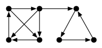
Figure 1: The orientation shown is an egalitarian orientation. In this graph all nodes are in the top ring. However, only the nodes in $K_{4}$ are in the densest subgraph.

2.2 Interpretation of density rank

We can interpret orientations as assigning responsibility: if an edge is oriented from node $a$ to node $b$, we can view node $b$ as being responsible for that connection. Indeed several allocation problems are modelled this way [11, 2, 42, 3, 19]. Put another way, we can view a node as wishing to shirk as many of its duties (modelled by incident edges) by assigning these duties to its neighbors (by orienting the linking edge away from itself). Of course, every node wishes to shirk as many of its duties as possible. However, the topology of the network may prevent a node from shirking too many of its duties. In fact, the egalitarian orientation is the assignment in which every node is allowed to simultaneously shirk as many duties as allowed by the topology of the network. An example is given in Figure 2; although nodes $a$ and $b$ both have degree 7, in the star network (left) $a$ can shirk all of its duties, but in the clique network (right) $b$ can only shirk half of its duties. There is a clear difference between these two cases that is captured by the density rank of $a$ and $b$ that is not captured by the degree of $a$ and $b$. For example, if these were co-authorship networks, the star network may represent a network in which author $a$ only co-authors papers with authors who never work with anyone else whereas the clique network shows that author $b$ co-authors with authors who also collaborate with others. One may surmise that the work of author $b$ is more reliable or respected than the work of author $a$.

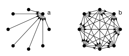
Figure 2: Two egalitarian orientations for networks with 8 nodes. This example generalizes to any number of nodes (Theorem 0.A.4).

Theorem 2.3

For a clique on $n$ nodes, there is an orientation where each node has indegree either $\lfloor n/2\rfloor$ or $\lfloor n/2\rfloor-1$.

A proof for Theorem 0.A.4 can be given by construction of such an egalitarian orientation (see Appendix 0.A) or by using a non-linear programming approach [36].

2.3 Relationship to $k$-cores

A $k$-core of a network is the maximal subnetwork whose nodes all have degree at least $k$ [40]. A $k$-core is found by repeatedly deleting nodes of degree less than $k$ while possible. For increasing values of $k$, the $k$-cores form a nesting hierarchy (akin to our density decomposition) of subnetworks $H_{0},H_{1},\ldots,H_{p}$ where $H_{i}$ is an $i$-core and $p$ is the smallest integer such that $G$ has an empty $(p+1)$-core. For networks generated by the $G_{n,p}$ model, most nodes are in the $p$-core [29, 37] For the preferential attachment model, all nodes except the initial nodes belong to the $c$-core, where $c$ is the number of edges connecting to each new node [1].

These observations are similar to those we find for the density distribution (Section 3) and many of the observations we make regarding the similarity of the degree and density distributions of real networks also hold for $k$-core decompositions [33]. However, the local definition of cores (depending only on the degree of a node) provides a much looser connection to density than the density decomposition, as we make formal in Lemma 7.

The density of the top core may be less then the density of the top ring. Also, there are graphs for which the densest subgraph is not contained in the top core (see Appendix 0.B).

Lemma 3

Given a core decomposition $H_{0},H_{1},\ldots,H_{k}$ of a network, the subnetwork formed by identifying the nodes in $\cup_{j>i}H_{j}$ and deleting the nodes in $\cup_{j<i}H_{j}$ has density in the range $[\frac{i}{2},i)$ for $|H_{i}|$ sufficiently large.

The proof of the above lemma can be found in Appendix 0.B.

3 The similarity of degree and density distributions

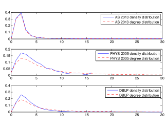
Figure 3: In the AS network nodes represent autonomous systems and two autonomous systems are connected if there is a routing agreement between them [49] (44,729 nodes and 170,735 edges). In the PHYS network nodes represent condensed matter physicists and two physicists are connected if they have at least one co-authored paper [34] (40,421 nodes and 175,692 edges). In the DBLP network, nodes represent computer scientists and two computer scientists are connected if they have at least one co-authored paper [48] (317,080 nodes and 1,049,866 edges). The (truncated) normalized density and degree distributions are displayed. The degree distributions have long diminishing tails. AS 2013 has 67 non-empty rings, but rings 31 through 66 contain less than 1.5% of the nodes; ring 67 contains 0.75% of the nodes. DBLP has 4 non-empty rings denser than ring 30 that are disconnected; rings 32, 40, 52 and 58 contain  0.02%, 0.01%, 0.03% and 0.04% of the nodes, respectively.

The normalized density $\boldsymbol{\rho}$ and degree $\boldsymbol{\delta}$ distributions for three networks (AS 2013, PHYS 2005, and DBLP) are given in Figure 3, illustrating the similarity of the distributions. We quantify the similarity between the density and degree distributions of these networks using the Bhattacharyya coefficient, $\beta$ [8]. For two normalized $\mathbf{p}$ and $\mathbf{q}$, the Bhattacharyya coefficient is:

$$\beta(\mathbf{p},\mathbf{q})=\sum_{i}\sqrt{p_{i}\cdot q_{i}}.$$

$\beta(\mathbf{p},\mathbf{q})\in[0,1]$ for normalized, positive distributions; $\beta(\mathbf{p},\mathbf{q})=0$ if and only if $\mathbf{p}$ and $\mathbf{q}$ are disjoint; $\beta(\mathbf{p},\mathbf{q})=1$ if and only if $\mathbf{p}=\mathbf{q}$. We denote the Bhattacharyya coefficient comparing the normalized density $\boldsymbol{\rho}$ and degree $\boldsymbol{\delta}$ distributions, $\beta(\boldsymbol{\rho},\boldsymbol{\delta})$ for a network $G$ by $\beta_{\rho\delta}(G)$. Specifically,

$$\beta_{\rho\delta}(G)=\beta(\boldsymbol{\rho},\boldsymbol{\delta})=\sum_{i}\sqrt{\rho_{i}\cdot\delta_{i}}$$

where $\rho_{i}$ is the fraction of nodes in the $i^{th}$ ring of the density decomposition of $G$ and $\delta_{i}$ is the fraction of nodes of total degree $i$ in $G$; we take $\rho_{i}=0$ for $i>k$ where $k$ is the maximum ring index. Refer to Figure 4. For all the networks in our data set, $\beta_{\rho\delta}>0.78$. Note that if we exclude the Gnutella and Amazon networks, $\beta_{\rho\delta}>0.9$. We point out that the other networks are self-determining in that each relationship is determined by at least one of the parties involved. On the other hand, the Gnutella network is highly structured and designed and the Amazon network is a is a one-mode projection of the buyer-product network (which is in turn self-determining).

Perhaps this is not surprising, given the close relationship between density and degree; one may posit that the density distribution $\boldsymbol{\rho}$ simply bins the degree distribution $\boldsymbol{\delta}$. However, note that a node’s degree is its total degree in the undirected graph, whereas a node’s rank is within one of its indegree in an egalitarian orientation. Since the total indegree to be shared amongst all the nodes is half the total degree of the network, we might assume that, if the density distribution is a binning of the degree distribution, the density rank of a node of degree $d$ would be roughly $d/2$. That is, we may expect that the density distribution is halved in range and doubled in magnitude ($\rho_{i}\approx 2{\delta}_{2i}$). If this is the case, then

$$\beta({\boldsymbol{\rho}},\boldsymbol{\delta})\approx\sum_{d}\sqrt{\rho_{i}\delta_{i}}\approx\sum_{d}\sqrt{2\delta_{d}{\delta}_{2d}}.$$

If we additionally assume that our network has a power-law degree distribution such as $\delta_{x}\varpropto 1/x^{3}$,

$$\beta({\boldsymbol{\rho}},{\boldsymbol{\delta}})\approx\int_{1}^{\infty}\sqrt{\frac{2}{x^{3}}\left(2{\frac{2}{(2x)^{3}}}\right)}\mathrm{d}x=0.5$$

(after normalizing the distributions and using a continuous approximation of $\beta$). Even with these idealized assumptions, this does not come close to explaining $\beta_{\rho\delta}$ being in excess of 0.78 for the networks in our data set. Further, for many synthetic networks $\beta_{\rho\delta}$ is small, as we discuss in the next section. We note that this separation between similarities of density and degree distributions for the empirical networks and synthetic networks can be illustrated with almost any divergence or similarity measure for a pair of distributions.

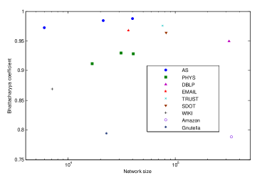
Figure 4: Similarity ($\beta_{\rho\delta}$) of density and degree distributions for 9 diverse networks. We introduced AS, PHYS, and DBLP in Figure 3. In the EMAIL network nodes represent Enron email addresses and two addresses are connected if there has been at least one email exchanged between them [22] (36,692 nodes and 183,831 edges). In the TRUST network nodes represent epinions.com members and two members are connected if one trusts the other [41] (75,879 nodes and 405,740 edges). In the SDOT network nodes represent slashdot.org members and two members are connected if they are friends or foes [28] (82,168 nodes and 504, 230 edges). In the WIKI network nodes represent wikipedia.org users and two users are connected if one has voted for the other to be in an administrative role [26] (7,115 nodes and 103,689 edges). In the Amazon network nodes represent products and two products are connected if they are frequently purchased together [48] (334,863 nodes and 925,872 edges). In the Gnutella network nodes represent network hosts and two hosts are connected if they share files [38] (22,687 nodes and 54,704 edges). EMAIL , TRUST, and WIKI are naturally directed networks. For these networks, we ignore direction and study the underlying undirected networks. Notice that both the Amazon and Gnutella networks are highly structured. It is not surprising that these networks would have a weaker connection between the density and degree distributions.

3.1 The dissimilarity of degree and density distributions of random networks

In contrast to the measurably similar degree and density distributions of real networks, the degree and density distributions are measurably dissimilar for networks produced by many common random network models; including the preferential attachment (PA) model of Barabasi and Albert [6] and the small world (SW) model of Watts and Strogatz [44]. We use $\tilde{\beta}_{\rho\delta}(M)$ to denote the Bhattacharyya coefficient comparing the expected degree and density distributions of a network generated by a model $M$.

Preferential attachment networks

In the PA model, a small number, $n_{0}$, of nodes seed the network and nodes are added iteratively, each attaching to a fixed number, $c$, of existing nodes. Consider the orientation where each added edge is directed toward the newly added node; in the resulting orientation, all but the $n_{0}$ seed nodes have indegree $c$ and the maximum indegree is $c$. At most $cn_{0}$ path reversals will make this orientation egalitarian, and, since $cn_{0}$ is typically very small compared to $n$ (the total number of nodes), most of the nodes will remain in the densest ring $R_{c}$. Therefore PA networks have nearly-trivial density distributions: $\rho_{c}\approx 1$. On the other hand the expected fraction of degree $c$ nodes is $2/(c+2)$ [5]. Therefore $\tilde{\beta}_{\rho\delta}(\mbox{PA})\approx\sqrt{2/(c+2)}$.

Small-world networks

A small-world network is one generated from a $d$-regular networkby reconnecting (uniformly at random) at least one endpoint of every edge with some probability. For probabilities close to 0, a network generated in this way is close to $d$-regular; for probabilities close to 1, a network generated this way approaches one generated by the random-network model ($G_{n,p}$) of Erdös and Rényi [13]. In the first extreme, $\tilde{\beta}_{\rho\delta}(SW)=0$ (Lemma 4 below) because all the nodes have the same degree and the same rank. As the reconnection probability increases, nodes are not very likely to change rank while the degree distribution spreads slightly. In the second extreme, the highest rank of a node is $\lfloor c/2\rfloor+1$ [47] and, using an observation of the expected size of the densest subnetwork, with high probability nearly all the nodes have this rank. It follows that

$$\tilde{\beta}_{\rho\delta}(G_{n,p})\approx\sqrt{\frac{c^{c/2}}{e^{-c}(c/2)!}},$$

which approaches 0 very quickly as $c$ grows. We verified this experimentally finding that $\tilde{\beta}_{\rho\delta}(G_{n,p})<0.5$ for $c\geq 5$.

Lemma 4

For $d\geq 3$, $\beta_{\rho\delta}(G)=0$ for any $d$-regular network $G$ with $d\geq 3$.

Proof

We argue that $\rho_{d}=0$, proving the lemma since $\delta_{d}=1$ for a $d$-regular network. For a contradiction, suppose $\rho_{d}>0$. Then $|R_{d}|=x$ for some $x>0$, where $R_{d}$ is the set of nodes of $G$ in the $d^{th}$ ring of $G$’s density decomposition. Note that the highest rank node in $G$ has rank at most $d$, since there are no nodes with degree $>d$. Let $H$ be the subnetwork of $H$ containing all the nodes of $R_{d}$ and all the edges of $G$ both of whose endpoints are in $R_{d}$. $H$ has at least one node of indegree $d$ and all other nodes have indegree at least $d-1$; therefore $H$ must have at least $d+(x-1)(d-1)$ edges. On the other hand, the total degree of every node in $H$ is at most $d$, so $H$ has at most $dx/2$ edges. We must have $d+(x-1)(d-1)\leq dx/2$, which is a contradiction for $d\geq 3$ and $x>0$.

4 Conclusion

We have introduced the density decomposition and summarized the decomposition with the density distribution. We found that the hierarchy of vertices within this decomposition are partitioned according to the density of the induced subgraphs. We found that the density and degree distributions are remarkably similar in real graphs and dissimilar in synthetic networks. In the appendix we discuss using the density distribution to build more realistic random graph models.

Appendix 0.A Proofs

In this section we include proofs for theorems in Sections 2.1 and 2.2.

Lemma 5

The density of the subnetwork induced by the nodes in $R_{k}$ is in the range $(k-1,k]$.

Proof

All nodes in $R_{k}$ have indegree $k$ or $k-1$ in $G$. Since any edge incident to a node in $R_{k}$ but not in $G[R_{k}]$ is directed out of $R_{k}$ in $G$, the indegree of every node in $G[R_{k}]$ is $k$ or $k-1$. Let $n_{k}$ be the number of nodes of indegree $k$ in $G[R_{k}]$ and $n_{k-1}$ be the number of nodes of degree $k-1$ in $G[R_{k-1}]$. Therefore, the number of edges in $G[R_{k}]$ is $kn_{k}+(k-1)n_{k-1}$ and:

$$\text{density}(G[R_{k}])={\frac{kn_{k}+(k-1)n_{k-1}}{n_{k}+n_{k-1}}}\leq k$$

Since there is at least one node of indegree $k$ in $G[R_{k}]$, $n_{k}>0$. Therefore:

$${\frac{kn_{k}+(k-1)n_{k-1}}{n_{k}+n_{k-1}}}=\frac{(k-1)(n_{k}+n_{k-1})+n_{k}}{n_{k}+n_{k-1}}>k-1$$

Lemma 6

The density of a densest subnetwork is in the range $(k-1,k]$.

Proof

Let $H$ be a densest subnetwork and let each edge of $H$ inherit the orientation of the same edge in an egalitarian orientation of $G$. Every node of $H$ has indegree at most $k$ (when restricted to $H$). Therefore

$$\text{density}(H)\leq\frac{n_{H}k}{n_{H}}\leq k$$

where $n_{H}$ is the number of nodes in $H$. Furthermore, by Lemma 5, the density of $G[R_{k}]$ is greater than $k-1$ and so the densest subnetwork must be at least this dense.

Theorem 0.A.1

The density decomposition is unique.

Proof

The maximum indegree of two egalitarian orientations for a given network is the same [11, 3, 42]. Suppose, for a contradiction, that there are two egalitarian orientations (red and blue) for $G$, resulting in density decompositions $R_{0},R_{1},\dots R_{k}$ and $B_{0},B_{1},\dots B_{k}$, respectively. Let $i$ be the largest index such that $R_{i}\neq B_{i}$.

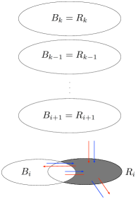
Figure 5: Edges incident to $S$ (grey region) in the proof of Theorem 0.A.1 in red and blue orientations. $S$ is the region in gray. Unoriented edges indicate that the orientation could be in either direction.

We compare the orientation of the edges with one endpoint in $S=R_{i}\setminus B_{i}$ between the two orientations (illustrated in Figure 5). Since the orientations are egalitarian:

1. All the edges between $B_{i}$ and $S$ are directed into $S$ in the blue orientation.

2. All the edges between $S$ and $\{\cup_{j=i+1}^{k}R_{j}\}\setminus S$ are directed into $S$ with respect to both red and blue orientations.

3. All edges between $S$ and $\{\cup_{j=0}^{i-1}R_{j}\}\setminus S$ are directed out of $S$ with respect to the red orientation.

Based on these orientations, we have:

Observation 0.A.2

The number of edges directed into $S$ in the blue orientation is at least the number of edges directed into $S$ in the red orientation.

We will show that $R_{i}\subseteq B_{i}$; symmetrically $B_{i}\subseteq R_{i}$, completing the theorem.

With respect to the blue orientation, all nodes in $S$ have indegree strictly less than $i$. Further, by Observation 0.A.2, the total indegree shared amongst the nodes in $S$ with respect to the red orientation is at most that of the blue orientation. Since all nodes in $S$ have indegree $i$ or $i-1$ with respect to the red orientation, and, by Observation 0.A.2, the total indegree shared amongst the nodes in $S$ with respect to the red orientation is at most that of the blue orientation, all nodes in $S$ have indegree $i-1$ with respect to the red orientation.

In order for every node in $S$ to have indegree $i-1$ in the red orientation, all nodes that are directed into $S$ in the blue orientation, must also be directed into $S$ in the red orientation; in particular this is true about the edges between $S$ and $R_{i}\setminus S$. Therefore, none of the nodes in $S$ (which have indegree $i-1$) reaches a node of $R_{i}\setminus S$ of indegree $i$ with respect to the red orientation. This contradicts the definition of $R_{i}$; therefore $S$ must be empty.

The following theorem relies on the fact that the density decomposition is unique and proves Property D3.

Theorem 0.A.3

The densest subnetwork of a network $G$ is induced by a subset of the nodes in the densest ring of $G$.

Proof

First note that the densest subnetwork is an induced subnetwork, for otherwise, the subnetwork would be avoiding including edges that would strictly increase the density. Let $S$ be a set of nodes that induces a densest subnetwork of $G$. Consider a density decomposition of $G$ and let $k$ be the maximum rank of a node in $G$. Let $S_{k}=S\cap R_{k}$ and let $\bar{S}_{k}=S\setminus S_{k}$.

Let $A$ be the set of edges in $G[S_{k}]$, let $C$ be the set of edges in $G[\bar{S}_{k}]$, and let $B$ be the edges of $G[S]$ that are neither in $G[S_{k}]$ or $G[\bar{S}_{k}]$. We get

$$|B|+|C|\leq(k-1)|\bar{S}_{k}|$$ (1)

because all the edges in $B$ and $C$ have endpoints in $\bar{S}_{k}$ and all the nodes in $\bar{S}_{k}$ have indegree at most $k-1$ in the egalitarian orientation of $G$.

$$\text{density}(G[S])=\frac{|A|+|B|+|C|}{|S_{k}|+|\bar{S}_{k}|}$$ (2)

$$\text{density}(G[S_{k}]) = \frac{|A|}{|S_{k}|}$$

$$= \frac{\text{density}(G[S])(|S_{k}|+|\bar{S}_{k}|)-(|B|+|C|)}{|S_{k}|}\qquad\text{using Equation\leavevmode\nobreak\ (\ref{eq:dH})}$$

$$= \text{density}(G[S])+\frac{\text{density}(G[S])|\bar{S}_{k}|-(|B|+|C|)}{|S_{k}|}$$

$$\geq \text{density}(G[S])+\frac{\text{density}(G[S])|\bar{S}_{k}|-(k-1)|\bar{S}_{k}|}{|S_{k}|}\qquad\text{by Inequality\leavevmode\nobreak\ (\ref{eq:BC})}$$

$$> \text{density}(G[S])+\frac{(k-1)|\bar{S}_{k}|-(k-1)|\bar{S}_{k}|}{|S_{k}|}\qquad\text{by Lemma\leavevmode\nobreak\ \ref{lem:dense_between_k_k_1}}$$

$$= \text{density}(G[S])$$

Therefore, removing the nodes of $G[S]$ that are not in $R_{k}$ produces a network of strictly greater density.

Theorem 0.A.4

For a clique on $n$ nodes, there is an orientation where each node has indegree either $\lfloor n/2\rfloor$ or $\lfloor n/2\rfloor-1$.

Proof

Give the nodes of the clique an ordering, $v_{1},v_{2},\dots v_{n}$. Orient the edges between $v_{1}$ and $v_{2},\dots,v_{\lfloor n/2\rfloor+1}$ toward $v_{1}$ and edges between $v_{1}$ and $v_{\lfloor n/2\rfloor+2},\dots v_{n}$ toward $v_{\lfloor n/2\rfloor+2},\dots v_{n}$. Clearly $v_{1}$ has indegree $\lfloor n/2\rfloor$. Similarly, for $v_{2}$: Orient the edges between $v_{2}$ and $v_{3},\dots,v_{\lfloor n/2\rfloor+2}$ toward $v_{2}$ and edges between $v_{2}$ and $v_{\lfloor n/2\rfloor+3},\dots v_{n}$ toward $v_{\lfloor n/2\rfloor+3},\dots v_{n}$. Clearly $v_{2}$ has indegree $\lfloor n/2\rfloor$. Continue in this fashion until $v_{n}$. It is immediate that $v_{1},v_{2},\dots v_{\lfloor n/2\rfloor}$ have indegree $\lfloor n/2\rfloor$. Now for the remaining nodes: Consider $v_{i}$, ${\lfloor n/2\rfloor}<i\leq n$. $v_{i}$ has $n-i$ incoming edges from nodes $v_{i+1},\dots v_{n}$ and also ${i-\lfloor n/2\rfloor-1}$ incoming edges from $v_{1},\dots,v_{i-\lfloor n/2\rfloor-1}$. Therefore $v_{i}$ has indegree $\lfloor n/2\rfloor-1$. Therefore all nodes in the clique have indegree $\lfloor n/2\rfloor$ or $\lfloor n/2\rfloor-1$. Clearly such an orientation is egalitarian.

Appendix 0.B $k$-cores

See Figure 7 for an example of a graph in which the densest subgraph is not contained in the top core. Further, while the core decomposition of a network can be found in time linear in the number of edges [30, 7, 12] as opposed to the quadratic time required for the density decomposition [11], core decompositions do not lend themselves to a framework for building synthetic networks, since it is not clear how to generate a $p$-core at random, whereas density decompositions do.

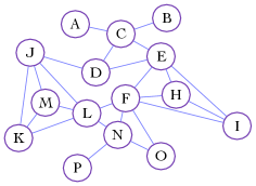
(a)

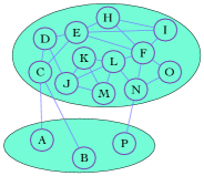
(b)

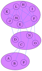
(c)

Figure 6: The top ring (Figure 6b) contains vertices $I,K,L,M,C,D,E,H,F,J,N$ and $O$ but $C,D,N,$ and $O$ are not in the top core (Figure 6c). The density of the subgraph induced by the top ring is $21/12=1.75$ while the density of the subgraph induced by the top core is $13/8=1.625$.

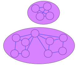
Figure 7: Core 3, the top core, has density 1.5. The densest subgraph is the subgraph induced by all vertices in core 2 and has density 1.56.

Recall that identifying the nodes in $\cup_{j>i}R_{j}$ and deleting the nodes in $\cup_{j<i}R_{j}$ leaves a network $G$ whose density is in the range $(i-1,i]$ (for $|R_{i}|$ sufficiently large). We find that the bound on density for the corresponding cores is much looser.

Lemma 7

Given a core decomposition $H_{0},H_{1},\ldots,H_{k}$ of a network, the subnetwork formed by identifying the nodes in $\cup_{j>i}H_{j}$ and deleting the nodes in $\cup_{j<i}H_{j}$ has density in the range $[\frac{i}{2},i)$ for $|H_{i}|$ sufficiently large.

Proof

Let $n$ be the number of nodes in the described subnetwork: $n=|H_{i}|+1$. Let $d$ be the degree of the node resulting from the identification of $\cup_{j>i}H_{j}$. Since every node in $H_{i}$ has degree at least $i$ in the subnetwork, the density of the subnetwork is at least ${{1\over 2}(i\cdot n+d)}\over n$, from which the lower bound of the lemma follows since $d\geq 0$. This lower bound is also tight when $H_{i}$ induces an $i$-regular network.

Further, the $i$-core is witnessed by iteratively deleting nodes of degree at most $i$ while such nodes exist. The subnetwork will have the greatest density (the most edges) if each deletion removes a node of degree exactly $i$. Then the subnetwork has density at most $i\cdot(n-1)\over n$.

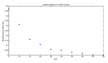
Figure 8:

Appendix 0.C Random networks with given density distributions

Based on the observation that real networks have similar density and degree decompositions and that many synthetic networks have dissimilar density and degree decompositions, we develop an abstract model, that, given a particular density distribution, produces a network having that density distribution (Section 0.C). Applied naïvely, given a density distribution of a real network, this model generates networks with realistic average path lengths (average number of hops between pairs of nodes) and degree distributions; that is similar to the given real network (Section 0.C.2). In addition to having short average path lengths, large-scale, real networks also tend to have high clustering coefficients [35]. The clustering coefficient of a node $v$ is the ratio of the number of pairs of neighbors of $v$ that are connected to the number of pairs of neighbors of $v$; the clustering coefficient of a network is the average clustering coefficient of its nodes. Our model, naïvely applied, unfortunately, but not surprisingly, results in networks with very low clustering coefficients. However, we show that applying the abstract model in a more sophisticated manner, using ideas from the small world model of Watts and Strogatz [44], results in much higher clustering coefficients (Section 0.C.3) suggesting that real networks may indeed be hierarchies of small worlds.

Our hierarchies of small worlds specification is just one way to tune our abstract model; our model is quite flexible allowing for the easy incorporation of other network generation techniques, which we discuss at the end of this paper. A key observation that distinguishes our model from other network models is our qualitatively different treatment of nodes. That is, our model begins by assigning nodes to levels of the density decomposition. This sets nodes qualitatively apart from each other; for example, a node assigned to a dense level of the decomposition is treated very differently from a node assigned to a sparse level of the decomposition.

Unlike our model, other network models, such as the small worlds model and the classic random graph model ($G_{n,p}$), treat each node in the same way [44]. In the preferential attachment model, in which nodes are attached one at a time to some fixed number of existing nodes [6], one may argue that nodes are treated differently since they arrive to the network at different times. However, when each node arrives, it is treated the same way as nodes before it. Similarly more recent network models, such as the affiliation network [25], community-guided attachment and forest-fire models [27], nodes are not distinguished from one another in a fixed way. We posit that in order to generate realistic networks, in particular networks exhibiting the rich density hierarchy we have observed in all the networks we have tested, one must assign nodes to classes and treat those classes differently. There are existing models that treat nodes qualitatively differently as we do. In the fitness, or Bianconi-Barabási model, each node has an intrinsic value, or “fitness” [9]. As a network produced by this model evolves, nodes with higher fitness are more likely to gain additional edges. In the planted partition model the nodes of the graph are divided into $\ell$ groups of size $\ell/|V|$, two nodes in the same group are connected with probability $p$ and two nodes from different groups are connected with probability $r<p$ [20]. Thus nodes in different groups are treated qualitatively differently.

Data sets

We note that our conclusions on the similarity of density and degree distributions of a given network are stronger for self-determining networks or those networks that represent relationships, each of which is determined by at least one of the parties in this relationship. Perhaps the clearest example of a self-determining network is a social network in which nodes represent people and an edge represents a friendship between two people. On the other hand a network representing the transformers and power lines that connect them in a power grid is clearly not self-determining as the transformers themselves do not determine which other transformers they are connected to, but a power authority does. For comparison, we include two non-self-determining networks.

Table 1 provides a list of the real networks that we study.

Self-determining networks
Name	Nodes	$\#$ Nodes	Edges	$\#$ Edges	Source
AS	autonomous systems	44,729	routing agreements	170,735	[49]
DBLP	computer scientists	317,080	at least one co-authored paper	1,049,866	[48]
Enron	email addresses	36,692	at least one email exchanged	183,831	[22]
Epinions	epinions.com members	75,879	self-indicated trust	405,740	[41]
Facebook	Facebook user	4,039	Facebook friends	88234	[31]
PHYS	condensed matter physicists	40,421	at least one co-authored paper	175,692	[34]
Slashdot	slashdot.org members	82,168	indication of friend or foe	504,230	[28]
Wikivote	wikipedia.org users	7,115	votes for administrator role	103,689	[26]
Non-self-determining networks
Name	Nodes	$\#$ Nodes	Edges	$\#$ Edges	Source
Amazon	products	334,863	pairs of frequently co-purchased items	925,872	[48]
Gnutella	network hosts	22,687	connections for file sharing	54,705	[38]

Table 1: Network data sets. For naturally directed networks (Enron, Epinions and Wikivote), we ignore the directions and study the underlying undirected network. We likewise ignore edge annotations (e.g. friend or foe in the Slashdot network). We use three snapshots of the AS network (from 1999, 2005 and 2011) and three snapshots of the PHYS network (for papers posted to arxiv.org prior to 1999, 2003 and 2005). Note that the structure of the Gnutella network is given by external system design specifications.

0.C.1 Models

Given a density distribution $\boldsymbol{\rho}$, we can generate a network with $n$ nodes having this density distribution using the following abstract model:

1:density distribution $\boldsymbol{\rho}$ and target size $n$

2:a network $G$ with $n$ nodes and density distribution $\boldsymbol{\rho}$

3:Initialize $G$ to be a network with empty node set $V$

4:for $i=|\boldsymbol{\rho}|,\ldots,0$ do

5:     $R_{i}\leftarrow$ set of $\lfloor\rho_{i}n\rfloor$ nodes

6:     add $R_{i}$ to $V$

7:     for each node $v\in R_{i}$ do

8:         connect $i$ nodes of $V$ to $v$      

Using this generic model, we propose two specific models, the random density distribution model (RDD) and the hierarchical small worlds model (HSW), by specifying how the neighbors are selected in Step 8. First we show that this abstract model does indeed generate a network with the given density distribution:

Lemma 8

The network resulting from the abstract model has density distribution $\boldsymbol{\rho}$.

Proof

We argue that the orientation given by, in Step 8, directing the added edges into $v$ is egalitarian. For a contradiction, suppose there is a reversible path. There must be an edge on this path from a node $x$ to a node $y$ such that the in-degree of $y$ is strictly greater than the degree of $x$. By construction, then, $x$ was added after $y$ and so an edge between $x$ and $y$ must oriented into $x$, contradicting the direction required by the reversible path.

Finally, since the nodes in set $R_{i}$ have indegree $i$ according to this orientation, the orientation is a witness to a density decomposition of the given distribution.

Notice that in this construction, nodes in $R_{i}$ will have indegree $i$ while a network with the same density decomposition may have nodes in $R_{i}$ with indegree $i-1$. We could additionally specify the number of nodes in $R_{i}$ that have indegree $i$ and indegree $i-1$; this would additionally require ensuring that there is an egalitarian orientation in which all the nodes destined to have indegree $i-1$ in $R_{i}$ reach nodes of indegree $i$ in $R_{i}$. We believe this is needlessly over-complicated and, indeed, over-specification that will have little affect on the generation large realistic networks.

Further notice that this abstract model may generate a network that is not simple. Without further constraint, in Step 8, $v$ may connect to itself (introducing a self-loop) or to a node that $v$ is already connected to (introducing parallel edges). We adopt a simple technique used for generating $d$-regular networks [32]: we constrain the choice in Step 8 to nodes of $V$ that are not $v$ itself nor neighbors of $v$. McKay and Wormald prove this constraint still allows for uniformity of sampling of $d$-regular networks when $d$ is sufficiently small ($d=O(n^{1/3})$) [21]; likewise, since $i$ is small compared to $|R_{i}|$ for large networks, adopting this technique should not affect our sampling. In our two specific models, described below, we ensure the final network will be simple using this technique.

0.C.2 Random density distribution model

For the RDD model, we choose $i$ nodes from $V$ uniformly at random in Step 8. We use this to model four networks in our data set (AS, DBLP, EMAIL, and TRUST). For each given network, we generate another random network having the given network’s number of nodes and density distribution. Remarkably, although we are only specifying the distribution of the nodes over a density decomposition, the resulting degree distributions of the RDD networks are very similar to the original networks they are modeling. We use the Bhattacharyya coefficient to quantify the similarity between the normalized degree distribution of an RDD network and the normalized degree distribution of the original network; we denote this by $\beta_{\delta\delta}$ (to distinguish from our use of the Bhattacharyya coefficient to compare degree distributions to density distributions. For all four models, $\beta_{\delta\delta}>0.93$ (Figure 9). Further, the average path lengths of the RDD networks are realistic, within  2 of the average path lengths of the original networks (Figure 10).

However, the clustering coefficients of the RDD networks are unrealistically low (Figures 9 and 10). Upon further inspection, we find that, for example, the PHYS networks have many more edges between nodes of a common ring of its density decomposition than between rings as compared to the corresponding RDD model. For the RDD model, we can compute the expected fraction of edges that will have one endpoint in $R_{i}$ and one endpoint in $R_{j}$. Since there are $|R_{j}||R_{i}|$ such edges to choose from (for $j>i$) and at most $|R_{i}|(\frac{1}{2}(|R_{i}|-1)+\sum_{j>i}|R_{j}|))$ edges between $R_{i}$ and $R_{j}$ (for $j>i$), we would expect this fraction to be:

$$\frac{|R_{j}|}{\frac{1}{2}(|R_{i}|-1)+\sum_{j>i}|R_{j}|}\text{ for $j>i$ and }\frac{\frac{1}{2}(|R_{i}|-1)}{\frac{1}{2}(|R_{i}|-1)+\sum_{j>i}|R_{j}|}\text{ for $i=j$}$$ (3)

In Figure 11 we plot the difference between the actual fraction of edges connecting $R_{i}$ to $R_{j}$ in the PHYS networks with this expected fraction for all values of $j-i$. We see that when $j-i=0$, or for edges with both endpoints in the same ring, there is a substantially larger number of edges in the original networks than is being captured by our model. This provides one explanation for the low clustering coefficients produced by the RDD model.

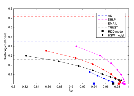
Figure 9: Clustering coefficient versus similarity of degree distribution (between models and original networks, $\beta_{\delta\delta}$) for RDD and HSW models. Measurements for the SW model networks are not shown as $\beta_{\delta\delta}<0.4$ for all networks generated. Dotted lines represent the clustering coefficients for the original networks.

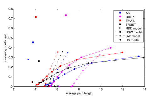
Figure 10: Clustering coefficient versus average path length for RDD, HSW, SW and DS models. Colors indicate the network being modelled. Squares denote the data for the original networks.

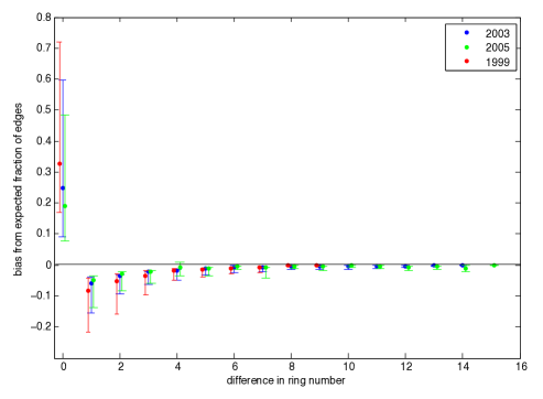
Figure 11: Range of difference between the actual fraction of edges connecting $R_{i}$ to $R_{j}$ and expected fraction (Equation (3)) over all $j\geq i$ as a function of $j-i$ for three PHYS networks. Error bars show max and min values of these differences and dots indicate the average.

0.C.3 Hierarchical small worlds model

We provide a more sophisticated model which addresses the unrealistically low clustering coefficients of the RDD model by generating a small world (SW) network among the nodes of each ring of the density decomposition. Recall that a SW network on $n$ nodes, average degree $d$ and randomization $p$ network is created as follows: order the nodes cyclically and connect each node to the $d$ nodes prior to it; with probability $p$ reconnect one endpoint of each edge to another node chosen uniformly at random. The SW model provides a trade-off between clustering coefficient and average path length: as $p$ increases, the clustering coefficient and the average path length decreases [44].

In the hierarchical small worlds (HSW) model, for nodes in $R_{i}$, we create a SW network on $|R_{i}|$ nodes and average degree $i$ in the same way, except for how we reconnect each edge with probability $p$. For an edge $uv$ where $u$ is a node within $d$ nodes prior to $v$ in the cyclic order, we select a node $x$ uniformly at random from $\cup_{j>i}R_{j}$ and replace $uv$ with $xv$. For the densest ring, we select a node uniformly at random from the densest ring.

This process is exactly equivalent to the following: order $R_{i}$ cyclically; for each $v\in R_{i}$, with probability $p$, connect each of the $i$ nodes before $v$ in this order to $v$; if $c\leq i$ neighbors for $v$ are selected in this way, select $i-c$ nodes uniformly at random from $\cup_{j>i}R_{j}$ (or $R_{i}$ if this is the densest ring) and connect these to $v$. Clearly, this is a specification of neighbor selection for Step 8 of the abstract model.

For the AS, DBLP, EMAIL, and TRUST networks in our data set, we generate a random network according to the HSW model that is of the same size and density distribution of the original network. We do so for $p=0.1,0.2,\ldots,0.9$. As with the SW model, the HSW model provides a similar trade-off between clustering coefficient and average path length (Figure 10), although the relationship is less strong. In addition, we observe a similar trade-off between $p$ and degree distribution: as $p$ increases, the degree distribution approaches that of the original network (Figure 9). This is in sharp contrast to the SW model which have degree distributions far from the original (normal vs. close to power law).

0.C.4 Comparing to the degree sequence model

We also compare our models (RDD and HSW) to a degree sequence (DS) model. For a given degree distribution or sequence (assignment of degree to each node), a DS model will generate a graph, randomly, having that degree sequence. We use the model of Viger and Latapy which generates a connected, simple graph by iteratively selecting neighbors for nodes (from highest remaining degree to be satisfied to lowest) and randomly shuffling to prevent the process from getting stuck (if no new neighbor exists that has not yet fulfilled its prescribed degree) [43]. As with RDD and HSW we generate a network using this DS model corresponding to the degree sequence of the AS, EMAIL, and TRUST networks. The clustering coefficients of the resulting networks are much lower than in the real networks (Figure 10); in the case of the AS network, this mismatch is less extreme, most likely because this network has an extremely long tail with a node with degree 4,171; many nodes would connect to these high degree nodes, providing an opportunity for clustering. The average path lengths are close to the original networks. Notably, the density distributions of the networks generated by the DS model are very similar to their degree distribution, all having $\beta_{\rho\delta}>0.9$.

These observations for the DS model add evidence to our proposal that in order to generate realistic networks, one must distinguish between types of nodes; doing so results in networks that resemble real networks. However, we must note that the DS model suffers from two drawbacks. First, the algorithms for generating such networks are much less efficient than our models (RDD and HSW, which run in linear time); in order to guarantee simplicity and connectivity, the reshuffling required incurs a large computational overhead, particularly when the degree sequence includes very high degree nodes (such as in the AS network). Second, the amount of information required to specify network generation via the DS model is much greater than our abstract model. In the former, the degree of every node must be specified, or at least the number of nodes having each degree. For example, the SLASH network has 457 unique degrees (and a maximum degree of 2553) while only having 61 non-empty rings in the density decomposition.

References

- [1] Jose Alvarez-Hamelin, Luca Dall’Asta, Alain Barrat, and Alessandro Vespignani. k-core decomposition of Internet graphs: hierarchies, self-similarity and measurement biases. Networks and Heterogeneous Media, 3(2):371, 2008.
- [2] Yuichi Asahiro, Jesper Jansson, Eiji Miyano, and Hirotaka Ono. Upper and lower degree bounded graph orientation with minimum penalty. In Proceedings in Computing: The Australasian Theory Symposium, pages 139–146, 2012.
- [3] Yuichi Asahiro, Eiji Miyano, Hirotaka Ono, and Kouhei Zenmyo. Graph orientation algorithms to minimize the maximum outdegree. International Journal of Foundations of Computer Science, 18(2):197–215, 2007.
- [4] Bahman Bahmani, Ravi Kumar, and Sergei Vassilvitskii. Densest subgraph in streaming and mapreduce. Proc. VLDB Endow., 5(5):454–465, January 2012.
- [5] Albert-László Barabási. Network Science. Cambridge University Press, Cambridge, 2016.
- [6] Albert-László Barabási and Réka Albert. Emergence of scaling in random networks. Science, 286(5439):509–512, 1999.
- [7] Vladimir Batagelj and Matjaz Zaversnik. An O(m) algorithm for cores decomposition of networks. Advances of Data Analysis and Classification, 5:129–145, 2011.
- [8] Anil Kumar Bhattacharyya. On a measure of divergence between two statistical populations defined by their probability distributions. Bull. Calcutta Math. Soc., 35:99–109, 1943.
- [9] Ginestra Bianconi and Albert-Laszlo Barabási. Competition and multiscaling in evolving networks. EPL (Europhysics Letters), 54(4):436, 2001.
- [10] Therese Biedl, Timothy Chan, Yashar Ganjali, Mohammad Taghi Hajiaghayi, and David R. Wood. Balanced vertex-orderings of graphs. Discrete Appl. Math., 148:27–48, April 2005.
- [11] Glencora Borradaile, Jennifer Iglesias, Theresa Migler, Antonio Ochoa, Gordon Wilfong, and Lisa Zhang. Egalitarian graph orientations. In Journal of Graph Algorithms and Applications, volume 21, pages 687–708, 2017.
- [12] Moses Charikar. Greedy approximation algorithms for finding dense components in a graph. In Proceedings of the Third International Workshop on Approximation Algorithms for Combinatorial Optimization, pages 84–95, London, UK, 2000. Springer-Verlag.
- [13] Paul Erdös and Alfréd Rényi. On random graphs, I. Publicationes Mathematicae (Debrecen), 6:290–297, 1959.
- [14] András Frank and A. Gyárfás. How to orient the edges of a graph? Colloquia Mathematica Societatis János Bolyai, 1:353–364, 1976.
- [15] Hubert de Fraysseix and Patrice Ossona de Mendez. Regular orientations, arboricity, and augmentation. In Proceedings of the DIMACS International Workshop on Graph Drawing, pages 111–118, London, UK, 1995. Springer-Verlag.
- [16] Giorgio Gallo, Michael Grigoriadis, and Robert Tarjan. A fast parametric maximum flow algorithm and applications. SIAM Journal on Computing, 18(1):30–55, February 1989.
- [17] David Gibson, Ravi Kumar, and Andrew Tomkins. Discovering large dense subgraphs in massive graphs. In Proceedings of the 31st international conference on very large data bases, pages 721–732. VLDB Endowment, 2005.
- [18] Andrew Goldberg. Finding a maximum density subgraph. Technical report, University of California at Berkeley, Berkeley, CA, USA, 1984.
- [19] Nicholas J. A. Harvey, Richard E. Ladner, László Lovász, and Tami Tamir. Semi-matchings for bipartite graphs and load balancing. Journal of Algorithms, 59:53–78, 2006.
- [20] Mark Jerrum and Gregory B. Sorkin. The metropolis algorithm for graph bisection. Discrete Applied Mathematics, 82(1–3):155 – 175, 1998.
- [21] Jeong Han Kim and Van H. Vu. Generating random regular graphs. In Proceedings of the thirty-fifth annual ACM symposium on Theory of computing, STOC ’03, pages 213–222, New York, NY, USA, 2003. ACM.
- [22] Bryan Klimt and Yiming Yang. Introducing the Enron Corpus. In First Conference on Email and Anti-Spam, 2004.
- [23] William F. Klostermeyer. Pushing vertices and orienting edges. Ars Combinatorial, 51:65–75, 1999.
- [24] Łukasz Kowalik. Approximation scheme for lowest outdegree orientation and graph density measures. In Proceedings of the 17th International Conference on Algorithms and Computation, ISAAC’06, pages 557–566, Berlin, Heidelberg, 2006. Springer-Verlag.
- [25] Silvio Lattanzi and D. Sivakumar. Affiliation networks. In Proceedings of the Forty-first Annual ACM Symposium on Theory of Computing, STOC ’09, pages 427–434, New York, NY, USA, 2009. ACM.
- [26] Jure Leskovec, Daniel Huttenlocher, and Jon Kleinberg. Signed networks in social media. In Proceedings of the SIGCHI Conference on Human Factors in Computing Systems, CHI ’10, pages 1361–1370, New York, NY, USA, 2010. ACM. http://snap.stanford.edu/data/.
- [27] Jure Leskovec, Jon Kleinberg, and Christos Faloutsos. Graphs over time: Densification laws, shrinking diameters and possible explanations. In Proceedings of the eleventh ACM SIGKDD International Conference on Knowledge Discovery in Data Mining, pages 177–187. ACM Press, 2005.
- [28] Jure Leskovec, Kevin Lang, Anirban Dasgupta, and Michael Mahoney. Community structure in large networks: Natural cluster sizes and the absence of large well-defined clusters. CoRR, abs/0810.1355, 2008. http://snap.stanford.edu/data/.
- [29] Tomasz Łuczak. Size and connectivity of the k-core of a random graph. Discrete Mathematics, 91(1):61–68, August 1991.
- [30] David W. Matula and Leland L. Beck. Smallest-last ordering and clustering and graph coloring algorithms. J. ACM, 30(3):417–427, July 1983.
- [31] Julian Mcauley and Jure Leskovec. Discovering social circles in ego networks. ACM Transactions on Knowledge Discovery from Data, 8(1):4:1–4:28, February 2014.
- [32] Brendan D. McKay and Nicholas C. Wormald. Uniform generation of random regular graphs of moderate degree. J. Algorithms, 11(1):52–67, February 1990.
- [33] Theresa Migler. The Density Signature. PhD thesis, Oregon State University, 2014.
- [34] Mark Newman. Fast algorithm for detecting community structure in networks. Phys. Rev. E, 69:066133, Jun 2004. http://www-personal.umich.edu/~mejn/netdata/.
- [35] Mark Newman. Networks: An Introduction. Oxford University Press, Inc., New York, NY, USA, 2010.
- [36] Jean-Claude Picard and Maurice Queyranne. A network flow solution to some nonlinear 0-1 programming problems, with applications to graph theory. Networks, 12:141–159, 1982.
- [37] Boris Pittel, Joel Spencer, and Nicholas Wormald. Sudden emergence of a giant k-core in a random graph. J. Comb. Theory Ser. B, 67(1):111–151, May 1996.
- [38] Matei Ripeanu, Ian Foster, and Adriana Iamnitchi. Mapping the Gnutella network: Properties of large-scale peer-to-peer systems and implications for system design. IEEE Internet Computing Journal, 6:2002, 2002. http://snap.stanford.edu/data/.
- [39] Barna Saha, Allison Hoch, Samir Khuller, Louiqa Raschid, and Xiao-Ning Zhang. Dense subgraphs with restrictions and applications to gene annotation graphs. In Proceedings of the 14th Annual international conference on Research in Computational Molecular Biology, RECOMB’10, pages 456–472, Berlin, Heidelberg, 2010. Springer-Verlag.
- [40] Stephen Seidman. Network structure and minimum degree. Social Networks, 5(3):269–287, 1983.
- [41] Maryam Tahajod, Azadeh Iranmehr, and Nasim Khozooyi. Trust management for semantic web. In Computer and Electrical Engineering, 2009. ICCEE ’09. Second International Conference, volume 2, pages 3–6, 2009. http://snap.stanford.edu/data/.
- [42] Venkat Venkateswaran. Minimizing maximum indegree. Discrete Appl. Math., 143:374–378, September 2004.
- [43] Fabien Viger and Matthieu Latapy. Efficient and simple generation of random simple connected graphs with prescribed degree sequence. In The Eleventh International Computing and Combinatorics Conference, pages 440–449. Springer, 2005.
- [44] Duncan Watts and Steven Strogatz. Collective dynamics of ‘small-world’ networks. Nature, 393(6684):409–10, 1998.
- [45] W. Wimmer. Ein Verfahren zur Verhinderung von Verklemmungen in Vermittlernetzen. http://www.worldcat.org/title/verfahren-zur-verhinderung-von-verklemmungen-in-vermittlernetzen/, October 1978.
- [46] Vaughan Wittorff. Implementation of constraints to ensure deadlock avoidance in networks, 2009. US Patent # 7,532,584 B2.
- [47] Pu Gao Xavier Pérez-Giménez and Cristiane Sato. Arboricity and spanning-tree packing in random graphs with an application to load balancing. In Proceedings of the Twenty-Fifth Annual ACM-SIAM Symposium on Discrete Algorithms, SODA ’14, pages 317–326. SIAM, 2014.
- [48] Jaewon Yang and Jure Leskovec. Defining and evaluating network communities based on ground-truth. In Proceedings of the ACM SIGKDD Workshop on Mining Data Semantics, MDS ’12, pages 3:1–3:8, New York, NY, USA, 2012. ACM. http://snap.stanford.edu/data/.
- [49] Yu Zhang. Internet AS-level Topology Archive. http://irl.cs.ucla.edu/topology/.