KR³: An Architecture for Knowledge Representation and Reasoning in Robotics

Abstract

This paper describes an architecture that combines the complementary strengths of declarative programming and probabilistic graphical models to enable robots to represent, reason with, and learn from, qualitative and quantitative descriptions of uncertainty and knowledge. An action language is used for the low-level (LL) and high-level (HL) system descriptions in the architecture, and the definition of recorded histories in the HL is expanded to allow prioritized defaults. For any given goal, tentative plans created in the HL using default knowledge and commonsense reasoning are implemented in the LL using probabilistic algorithms, with the corresponding observations used to update the HL history. Tight coupling between the two levels enables automatic selection of relevant variables and generation of suitable action policies in the LL for each HL action, and supports reasoning with violation of defaults, noisy observations and unreliable actions in large and complex domains. The architecture is evaluated in simulation and on physical robots transporting objects in indoor domains; the benefit on robots is a reduction in task execution time of $39\%$ compared with a purely probabilistic, but still hierarchical, approach.

1 Introduction

Mobile robots deployed in complex domains receive far more raw data from sensors than is possible to process in real-time, and may have incomplete domain knowledge. Furthermore, the descriptions of knowledge and uncertainty obtained from different sources may complement or contradict each other, and may have different degrees of relevance to current or future tasks. Widespread use of robots thus poses fundamental knowledge representation and reasoning challenges—robots need to represent, learn from, and reason with, qualitative and quantitative descriptions of knowledge and uncertainty. Towards this objective, our architecture combines the knowledge representation and non-monotonic logical reasoning capabilities of declarative programming with the uncertainty modeling capabilities of probabilistic graphical models. The architecture consists of two tightly coupled levels and has the following key features:

• An action language is used for the HL and LL system descriptions and the definition of recorded history is expanded in the HL to allow prioritized defaults.

• For any assigned objective, tentative plans are created in the HL using default knowledge and commonsense reasoning, and implemented in the LL using probabilistic algorithms, with the corresponding observations adding suitable statements to the HL history.

• For each HL action, abstraction and tight coupling between the LL and HL system descriptions enables automatic selection of relevant variables and generation of a suitable action policy in the LL.

In this paper, the HL domain representation is translated into an Answer Set Prolog (ASP) program, while the LL domain representation is translated into partially observable Markov decision processes (POMDPs). The novel contributions of the architecture, e.g., allowing histories with prioritized defaults, tight coupling between the two levels, and the resultant automatic selection of the relevant variables in the LL, support reasoning with violation of defaults, noisy observations and unreliable actions in large and complex domains. The architecture is grounded and evaluated in simulation and on physical robots moving objects in indoor domains.

2 Related Work

Probabilistic graphical models such as POMDPs have been used to represent knowledge and plan sensing, navigation and interaction for robots (?; ?). However, these formulations (by themselves) make it difficult to perform commonsense reasoning, e.g., default reasoning and non-monotonic logical reasoning, especially with information not directly relevant to tasks at hand. In parallel, research in classical planning has provided many algorithms for knowledge representation and logical reasoning (?), but these algorithms require substantial prior knowledge about the domain, task and the set of actions. Many of these algorithms also do not support merging of new, unreliable information from sensors and humans with the current beliefs in a knowledge base. Answer Set Programming (ASP), a non-monotonic logic programming paradigm, is well-suited for representing and reasoning with commonsense knowledge (?; ?). An international research community has been built around ASP, with applications such as reasoning in simulated robot housekeepers and for representing knowledge extracted from natural language human-robot interaction (?; ?). However, ASP does not support probabilistic analysis, whereas a lot of information available to robots is represented probabilistically to quantitatively model the uncertainty in sensor input processing and actuation in the real world.

Researchers have designed cognitive architectures (?; ?; ?), and developed algorithms that combine deterministic and probabilistic algorithms for task and motion planning on robots (?; ?). Recent work has also integrated ASP and POMDPs for non-monotonic logical inference and probabilistic planning on robots (?). Some examples of principled algorithms developed to combine logical and probabilistic reasoning include probabilistic first-order logic (?), first-order relational POMDPs (?), Markov logic network (?), Bayesian logic (?), and a probabilistic extension to ASP (?). However, algorithms based on first-order logic for probabilistically modeling uncertainty do not provide the desired expressiveness for capabilities such as default reasoning, e.g., it is not always possible to express uncertainty and degrees of belief quantitatively. Other algorithms based on logic programming that support probabilistic reasoning do not support one or more of the desired capabilities: reasoning as in causal Bayesian networks; incremental addition of probabilistic information; reasoning with large probabilistic components; and dynamic addition of variables with different ranges (?). The architecture described in this paper is a step towards achieving these capabilities. It exploits the complementary strengths of declarative programming and probabilistic graphical models to represent, reason with, and learn from qualitative and quantitative descriptions of knowledge and uncertainty, enabling robots to automatically plan sensing and actuation in larger domains than was possible before.

3 KRR Architecture

This section describes our architecture’s HL and LL domain representations. The syntax, semantics and representation of the corresponding transition diagrams are described in an action language AL (?). Action languages are formal models of parts of natural language used for describing transition diagrams. AL has a sorted signature containing three sorts: statics, fluents and actions. Statics are domain properties whose truth values cannot be changed by actions, while fluents are properties whose truth values are changed by actions. Actions are defined as a set of elementary actions that can be executed in parallel. A domain property p or its negation $\lnot p$ is a domain literal. AL allows three types of statements:

$$\begin{array}[]{ll}a~{}~{}\mathbf{causes}~{}~{}l_{in}~{}~{}\mathbf{if}~{}p_{0},\ldots,p_{m}\qquad\qquad\qquad~{}~{}~{}~{}\textrm{(Causal law)}\\ l~{}~{}\mathbf{if}~{}~{}p_{0},\ldots,p_{m}\qquad\qquad\qquad\qquad~{}~{}~{}~{}~{}~{}~{}\textrm{(State constraint)}\\ \mathbf{impossible}~{}~{}a_{0},\ldots,a_{k}~{}~{}\mathbf{if}~{}~{}p_{0},\ldots,p_{m}\\ \qquad\qquad\qquad\qquad\qquad\qquad~{}~{}~{}\textrm{(Executability condition)}\end{array}$$

where $a$ is an action, $l$ is a literal, $l_{in}$ is a inertial fluent literal, and $p_{0},\ldots,p_{m}$ are domain literals. The causal law states, for instance, that action $a$ causes inertial fluent literal $l_{in}$ if the literals $p_{0},\ldots,p_{m}$ hold true. A collection of statements of AL forms a system/domain description.

As an illustrative example used throughout this paper, we will consider a robot that has to move objects to specific places in an indoor domain. The domain contains four specific places: office, main_library, aux_library, and kitchen, and a number of specific objects of the sorts: textbook, printer and kitchenware.

3.1 HL domain representation

The HL domain representation consists of a system description $\mathcal{D}_{H}$ and histories with defaults $\mathcal{H}$. $\mathcal{D}_{H}$ consists of a sorted signature and axioms used to describe the HL transition diagram $\tau_{H}$. The sorted signature: $\Sigma_{H}=\langle\mathcal{O},\mathcal{F},\mathcal{P}\rangle$ is a tuple that defines the names of objects, functions, and predicates available for use in the HL. The sorts in our example are: place, thing, robot, and object; object and robot are subsorts of thing. Robots can move on their own, but objects cannot move on their own. The sort object has subsorts such as textbook, printer and kitchenware. The fluents of the domain are defined in terms of their arguments:

$$loc(thing,place)$$ (2)

$$in\_hand(robot,object)$$

The first predicate states the location of a thing; and the second predicate states that a robot has an object.These two predicates are inertial fluents subject to the law of inertia, which can be changed by an action. The actions in this domain include:

$$move(robot,place)$$ (3)

$$grasp(robot,object)$$

$$putdown(robot,object)$$

The dynamics of the domain are defined using the following causal laws:

$$move(robot,Pl)~{}~{}\mathbf{causes}~{}~{}loc(robot,Pl)$$ (4)

$$grasp(robot,Ob)~{}~{}\mathbf{causes}~{}~{}in\_hand(robot,Ob)$$

$$putdown(robot,Ob)~{}~{}\mathbf{causes}~{}~{}\neg in\_hand(robot,Ob)$$

state constraints:

$$loc(Ob,Pl)~{}~{}\mathbf{if}~{}~{}loc(robot,Pl),~{}~{}in\_hand(robot,Ob)$$ (5)

$$\neg loc(Th,Pl_{1})~{}~{}\mathbf{if}~{}~{}loc(Th,Pl_{2}),~{}Pl_{1}\neq Pl_{2}$$

and executability conditions:

$$\mathbf{impossible}~{}~{}move(robot,Pl)~{}~{}\mathbf{if}~{}~{}loc(robot,Pl)$$ (6)

$$\mathbf{impossible}~{}~{}A_{1},~{}A_{2},~{}~{}\mathbf{if}~{}~{}A_{1}\neq A_{2}.$$

$$\mathbf{impossible}~{}~{}grasp(robot,Ob)~{}~{}\mathbf{if}~{}~{}loc(robot,Pl1),$$

$$~{}~{}~{}~{}~{}~{}~{}~{}~{}~{}~{}~{}~{}~{}~{}~{}~{}~{}~{}~{}loc(Ob,Pl2),Pl1\neq Pl2$$

$$\mathbf{impossible}~{}~{}grasp(robot,Ob)~{}~{}\mathbf{if}~{}~{}in\_hand(robot,Ob)$$

$$\mathbf{impossible}~{}~{}putdown(robot,Ob)~{}~{}\mathbf{if}~{}~{}\neg in\_hand(robot,Ob)$$

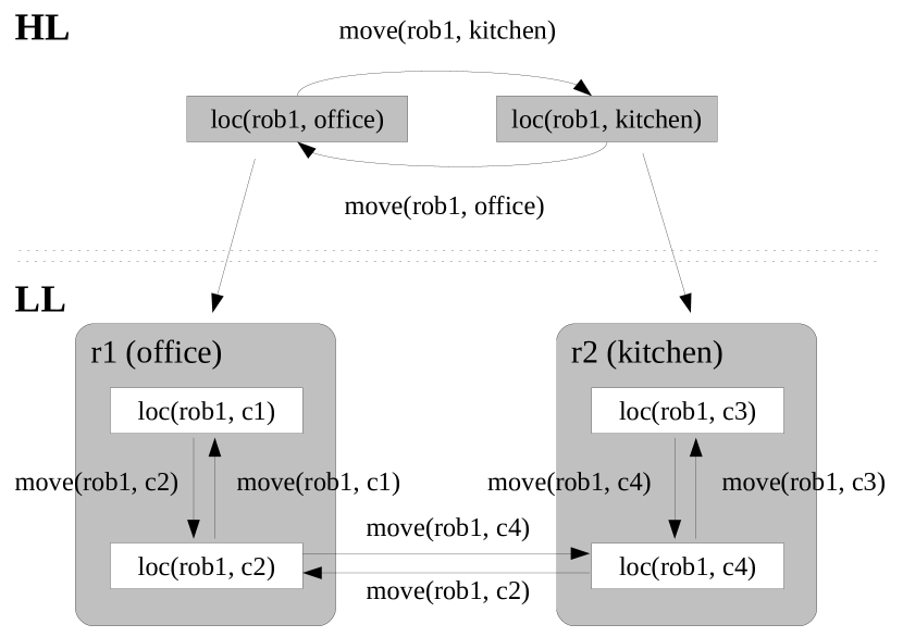
Figure 1: Illustrative example of state transitions in the HL and the LL of the architecture.

The top part of Figure 1 shows some state transitions in the HL; nodes include a subset of fluents (robot’s position) and actions are the arcs between nodes. Although $\mathcal{D}_{H}$ does not include the costs of executing actions, these are included in the LL (see Section 3.2).

Histories with defaults

A recorded history of a dynamic domain is usually defined as a collection of records of the form $obs(fluent,boolean,step)$ and $hpd(action,step)$. The former states that a specific fluent was observed to be true or false at a given step of the domain’s trajectory, and the latter states that a specific action happened (or was executed by the robot) at that step. In this paper, we expand on this view by allowing histories to contain (possibly prioritized) defaults describing the values of fluents in their initial states. A default $d(X)$ stating that in the typical initial state elements of class $c$ satisfying property $b$ also have property $p$ is represented as:

$$d(X)=\left\{\begin{array}[]{l}default(d(X))\\ head(d(X),p(X))\\ body(d(X),c(X))\\ body(d(X),b(X))\end{array}\right.$$ (7)

where the literal in the “head” of the default, e.g., $p(X)$ is true if all the literals in the “body” of the default, e.g., $b(X)$ and $c(X)$, hold true; see (?) for formal semantics of defaults. In this paper, we abbreviate $obs(f,true,0)$ and $obs(f,false,0)$ as $init(f,true)$ and $init(f,false)$ respectively.

Example 1

[Example of defaults]
Consider the following statements about the locations of textbooks in the initial state in our illustrative example. Textbooks are typically in the main library. If a textbook is not there, it is in the auxiliary library. If a textbook is checked out, it can be found in the office. These defaults can be represented as:

$$\begin{array}[]{ll}default(d_{1}(X))\\ head(d_{1}(X),loc(X,main\_library))\\ body(d_{1}(X),textbook(X))\end{array}$$ (8)

$$\begin{array}[]{l}default(d_{2}(X))\\ head(d_{2}(X),loc(X,aux\_library))\\ body(d_{2}(X),textbook(X))\\ body(d_{2}(X),\neg loc(X,main\_library))\end{array}$$ (9)

$$\begin{array}[]{l}default(d_{3}(X))\\ head(d_{3}(X),loc(X,office))\\ body(d_{3}(X),textbook(X))\\ body(d_{3}(X),\lnot loc(X,main\_library))\\ body(d_{3}(X),\lnot loc(X,aux\_library))\end{array}$$ (10)

A default such as “kitchenware are usually in the kitchen” may be represented in a similar manner. We first present multiple informal examples to illustrate reasoning with these defaults; Definition 3 (below) will formalize this reasoning. For textbook $tb_{1}$, history $\mathcal{H}_{1}$ containing the above statements should entail: $holds(loc(tb_{1},main\_library),0)$. A history $\mathcal{H}_{2}$ obtained from $\mathcal{H}_{1}$ by adding an observation: $init(loc(tb_{1},main\_library),false)$ renders the first default inapplicable; hence $\mathcal{H}_{2}$ should entail: $holds(loc(tb_{1},aux\_library),0)$. A history $\mathcal{H}_{3}$ obtained from $\mathcal{H}_{2}$ by adding an observation: $init(loc(tb_{1},aux\_library),false)$ entails: $holds(loc(tb_{1},office),0)$.

Consider history $\mathcal{H}_{4}$ obtained by adding observation: $obs(loc(tb_{1},main\_library),false,1)$ to $\mathcal{H}_{1}$. This observation should defeat the default $d_{1}$ in Equation 8 because if this default’s conclusion were true in the initial state, it would also be true at step $1$ (by inertia), which contradicts our observation. The book $tb_{1}$ is thus not in the main library initially. The second default will conclude that this book is initially in the auxiliary library—the inertia axiom will propagate this information and $\mathcal{H}_{4}$ will entail: $holds(loc(tb_{1},aux\_library),1)$.

The definition of entailment relation can now be given with respect to a fixed system description $\mathcal{D}_{H}$. We start with the notion of a state of transition diagram $\tau_{H}$ of $\mathcal{D}_{H}$ compatible with a description $\mathcal{I}$ of the initial state of history $\mathcal{H}$. We use the following terminology. We say that a set $S$ of literals is closed under a default $d$ if $S$ contains the head of $d$ whenever it contains all literals from the body of $d$ and does not contain the literal contrary to $d$’s head. $S$ is closed under a constraint of $\mathcal{D}_{H}$ if $S$ contains the constraint’s head whenever it contains all literals from the constraint’s body. Finally, we say that a set $U$ of literals is the closure of $S$ if $S\subseteq U$, $U$ is closed under constraints of $\mathcal{D}_{H}$ and defaults of $\mathcal{H}$, and no proper subset of $U$ satisfies these properties.

Definition 1

[Compatible initial states]
A state $\sigma$ of $\tau_{H}$ is compatible with a description $\mathcal{I}$ of the initial state of history $\mathcal{H}$ if:

• $\sigma$ satisfies all observations of $\mathcal{I}$,

• $\sigma$ contains the closure of the union of statics of $\mathcal{D}_{H}$ and the set $\{f:init(f,true)\in\mathcal{I}\}\cup\{\neg f:init(f,false)\in\mathcal{I}\}$.

Let $\mathcal{I}_{k}$ be the description of the initial state of history $\mathcal{H}_{k}$. States in Example 1 compatible with $\mathcal{I}_{1}$, $\mathcal{I}_{2}$, $\mathcal{I}_{3}$ must then contain $\{loc(tb_{1},main\_library)\}$, $\{loc(tb_{1},aux\_library)\}$, and $\{loc(tb_{1},office)\}$ respectively. There are multiple such states, which differ by the location of robot. Since $\mathcal{I}_{1}=\mathcal{I}_{4}$ they have the same compatible states. Next, we define models of history $\mathcal{H}$, i.e., paths of the transition diagram $\tau_{H}$ of $\mathcal{D}_{H}$ compatible with $\mathcal{H}$.

Definition 2

[Models]
A path $P$ of $\tau_{H}$ is a model of history $\mathcal{H}$ with description $\mathcal{I}$ of its initial state if there is a collection $E$ of $init$ statements such that:

• If $init(f,true)\in E$ then $\neg f$ is the head of one of the defaults of $\mathcal{I}$. Similarly, for $init(f,false)$.

• The initial state of $P$ is compatible with the description: $\mathcal{I}_{E}=\mathcal{I}\cup E$.

• Path $P$ satisfies all observations in $\mathcal{H}$.

• There is no collection $E_{0}$ of $init$ statements which has less elements than $E$ and satisfies the conditions above.

We will refer to $E$ as an explanation of $\mathcal{H}$. Models of $\mathcal{H}_{1}$, $\mathcal{H}_{2}$, and $\mathcal{H}_{3}$ are paths consisting of initial states compatible with $\mathcal{I}_{1}$, $\mathcal{I}_{2}$, and $\mathcal{I}_{3}$—the corresponding explanations are empty. However, in the case of $\mathcal{H}_{4}$, the situation is different—the predicted location of $tb_{1}$ will be different from the observed one. The only explanation of this discrepancy is that $tb_{1}$ is an exception to the first default. Adding $E=\{init(loc(tb_{1},main\_library),false)\}$ to $\mathcal{I}_{4}$ will resolve the problem.

Definition 3

[Entailment and consistency]

• Let $\mathcal{H}^{n}$ be a history of length $n$, $f$ be a fluent, and $0\leq i\leq n$ be a step of $\mathcal{H}^{n}$. We say that $\mathcal{H}^{n}$ entails a statement $Q=holds(f,i)$ ($\neg holds(f,i)$) if for every model $P$ of $\mathcal{H}^{n}$, fluent literal $f$ ($\neg f$) belongs to the $i$th state of $P$. We denote the entailment as $\mathcal{H}^{n}\models Q$.

• A history which has a model is said to be consistent.

It can be shown that histories from Example 1 are consistent and that our entailment captures the corresponding intuition.

Reasoning with HL domain representation

The HL domain representation ($\mathcal{D}_{H}$ and $\mathcal{H}$) is translated into a program in CR-Prolog, which incorporates consistency restoring rules in ASP (?; ?); specifically, we use the knowledge representation language SPARC that expands CR-Prolog and provides explicit constructs to specify objects, relations, and their sorts (?). ASP is a declarative language that can represent recursive definitions, defaults, causal relations, special forms of self-reference, and other language constructs that occur frequently in non-mathematical domains, and are difficult to express in classical logic formalisms (?). ASP is based on the stable model semantics of logic programs, and builds on research in non-monotonic logics (?). A CR-Prolog program is thus a collection of statements describing domain objects and relations between them. The ground literals in an answer set obtained by solving the program represent beliefs of an agent associated with the program; program consequences are statements that are true in all such belief sets. Algorithms for computing the entailment relation of AL and related tasks such as planning and diagnostics are thus based on reducing these tasks to computing answer sets of programs in CR-Prolog. First, $\mathcal{D}_{H}$ and $\mathcal{H}$ are translated into an ASP program $\Pi(\mathcal{D}_{H},\mathcal{H})$ consisting of direct translation of causal laws of $\mathcal{D}_{H}$, inertia axioms, closed world assumption for defined fluents, reality checks, records of observations, actions and defaults from $\mathcal{H}$, and special axioms for $init$:

$$holds(F,0)\leftarrow init(F,true)$$ (11)

$$\neg holds(F,0)\leftarrow init(F,false)$$

In addition, every default of $\mathcal{I}$ is turned into an ASP rule:

$$holds(p(X),0)\leftarrow c(X),~{}~{}holds(b(X),0),$$ (12)

$$\;{not}\;\neg holds(p(X),0)$$

and a consistency-restoring rule:

$$\neg holds(p(X),0)\stackrel{{\scriptstyle\,\,+}}{{\leftarrow}} c(X),~{}~{}holds(b(X),0)$$ (13)

which states that to restore consistency of the program one may assume that the conclusion of the default is false. For more details about the translation, CR-rules and CR-Prolog, please see (?).

Proposition 1

[Models and Answer Sets]
A path $P=\langle\sigma_{0},a_{0},\sigma_{1},\dots,\sigma_{n-1},a_{n}\rangle$ of $\tau_{H}$ is a model of history $\mathcal{H}^{n}$ iff there is an answer set $S$ of a program $\Pi(\mathcal{D}_{H},\mathcal{H})$ such that:

• A fluent $f\in\sigma_{i}$ iff $holds(f,i)\in S$,

• A fluent literal $\neg f\in\sigma_{i}$ iff $\neg holds(f,i)\in S$,

• An action $e\in a_{i}$ iff $occurs(e,i)\in S$.

The proposition reduces computation of models of $\mathcal{H}$ to computing answer sets of a CR-Prolog program. This proposition allows us to reduce the task of planning to computing answer sets of a program obtained from $\Pi(\mathcal{D}_{H},\mathcal{H})$ by adding the definition of a goal, a constraint stating that the goal must be achieved, and a rule generating possible future actions of the robot.

3.2 LL domain representation

The LL system description $\mathcal{D}_{L}$ consists of a sorted signature and axioms that describe a transition diagram $\tau_{L}$. The sorted signature $\Sigma_{L}$ of action theory describing $\tau_{L}$ includes the sorts from signature $\Sigma_{H}$ of HL with two additional sorts room and cell, which are subsorts of sort place. Their elements satisfy the static relation part_of(cell, room). We also introduce the static neighbor(cell, cell) to describe neighborhood relation between cells. Fluents of $\Sigma_{L}$ include those of $\Sigma_{H}$, an additional inertial fluent: searched(cell, object)—robot searched a cell for an object—and two defined fluents: found(object, place)—an object was found in a place—and continue_search(room, object)—the search for an object is continued in a room.

The actions of $\Sigma_{L}$ include the HL actions that are viewed as being represented at a higher resolution, e.g., movement is possible to specific cells. The causal law describing the effect of move may be stated as:

$$move(robot,Y)~{}~{}\mathbf{causes}~{}~{}\{loc(robot,Z):neighbor(Z,Y)\}$$ (14)

where $Y,Z$ are cells. This causal law states that moving to a cell can cause the robot to be in one of the neighboring cells. The LL includes an additional action search that enables robots to search for objects in cells; the corresponding causal laws and constraints may be written as:

$$search(cell,object)~{}~{}\mathbf{causes}~{}~{}searched(cell,object)$$ (15)

$$found(object,cell)~{}~{}\mathbf{if}~{}~{}searched(cell,object),$$

$$~{}~{}~{}~{}~{}~{}~{}~{}~{}~{}~{}~{}~{}~{}~{}~{}~{}~{}~{}~{}~{}~{}~{}~{}~{}~{}~{}~{}~{}~{}~{}~{}~{}~{}loc(object,cell)$$

$$found(object,room)~{}~{}\mathbf{if}~{}~{}part\_of(cell,room),$$

$$~{}~{}~{}~{}~{}~{}~{}~{}~{}~{}~{}~{}~{}~{}~{}~{}~{}~{}~{}~{}~{}~{}~{}~{}~{}~{}~{}~{}~{}~{}~{}~{}~{}~{}~{}~{}found(object,cell)$$

$$continue\_search(room,object)~{}\mathbf{if}~{}\lnot found(object,room),$$

$$~{}~{}~{}~{}~{}~{}~{}~{}~{}~{}~{}~{}~{}~{}~{}~{}~{}~{}~{}part\_of(cell,room),\lnot searched(cell,object)$$

We also introduce a defined fluent failure that holds iff the object under consideration is not in the room that the robot is searching—this fluent is defined as:

$$failure(object,room)~{}~{}\mathbf{if}~{}~{}loc(robot,room),$$ (16)

$$~{}~{}~{}~{}\lnot continue\_search(room,object),\lnot found(object,room)$$

This completes the action theory that describes $\tau_{L}$. The states of $\tau_{L}$ can be viewed as extensions of states of $\tau_{H}$ by physically possible fluents and statics defined in the language of LL. Moreover, for every HL state-action-state transition $\langle\sigma,a,\sigma^{\prime}\rangle$ and every LL state $s$ compatible with $\sigma$ (i.e., $\sigma\subset s$), there is a path in the LL from $s$ to some state compatible with $\sigma^{\prime}$.

Unlike the HL system description in which effects of actions and results of observations are always accurate, the action effects and observations in the LL are only known with some degree of probability. The state transition function $T:S\times A\times S^{\prime}\to[0,1]$ defines the probabilities of state transitions in the LL. Due to perceptual limitations of the robot, only a subset of the fluents are observable in the LL; we denote this set of fluents by $Z$. Observations are elements of $Z$ associated with a probability, and are obtained by processing sensor inputs using probabilistic algorithms. The observation function $O:S\times Z\to[0,1]$ defines the probability of observing specific observable fluents in specific states. Functions $T$ and $O$ are computed using prior knowledge, or by observing the effects of specific actions in specific states (see Section 4.1).

States are partially observable in the LL, and we introduce (and reason with) belief states, probability distributions over the set of states. Functions $T$ and $O$ describe a probabilistic transition diagram defined over belief states. The initial belief state is represented by $B_{0}$, and is updated iteratively using Bayesian inference:

$$B_{t+1}(s_{t+1})\propto O(s_{t+1},o_{t+1})\sum_{s}T(s,a_{t+1},s_{t+1})\cdot B_{t}(s)$$ (17)

The LL system description includes a reward specification $R:S\times A\times S^{\prime}\to\Re$ that encodes the relative cost or value of taking specific actions in specific states. Planning in the LL then involves computing a policy that maximizes the reward over a planning horizon. This policy maps belief states to actions: $\pi:B_{t}\mapsto a_{t+1}$. We use a point-based approximate algorithm to compute this policy (?). In our illustrative example, an LL policy computed for HL action move is guaranteed to succeed, and that the LL policy computed for HL action grasp considers three LL actions: move, search, and grasp. Plan execution in the LL corresponds to using the computed policy to repeatedly choose an action in the current belief state, and updating the belief state after executing that action and receiving an observation. We henceforth refer to this algorithm as “POMDP-1”.

Unlike the HL, history in the LL representation consists of observations and actions over one time step; the current belief state is assumed to be the result of all information obtained in previous time steps (first-order Markov assumption). In this paper, the LL domain representation is translated automatically into POMDP models, i.e., specific data structures for representing the components of $\mathcal{D}_{L}$ (described above) such that existing POMDP solvers can be used to obtain action policies.

We observe that the coupling between the LL and the HL has some key consequences. First, for any HL action, the relevant LL variables are identified automatically, improving the computational efficiency of computing the LL policies. Second, if LL actions cause different fluents, these fluents are independent. Finally, although defined fluents are crucial in determining what needs to be communicated between the levels of the architecture, they themselves need not be communicated.

3.3 Control loop

1

Input: The HL and LL domain representations, and the specific task for robot to perform.

2

3LL observations reported to HL history; HL initial state ($s^{H}_{init}$) communicated to LL.

4

5Assign goal state $s^{H}_{goal}$ based on task.

6

7Generate HL plan(s).

8

9if multiple HL plans exist then

10       Send plans to the LL, select plan with lowest (expected) action cost and communicate to the HL.

11      

12 end if

13

14if HL plan exists then

15      

16      for $a_{i}^{H}\in$ HL plan: $i\in[1,n]$ do

17            

18            Pass $a_{i}^{H}$ and relevant fluents to LL.

19            

20            Determine initial belief state over the relevant LL state space.

21            

22            Generate LL action policy.

23            

24            while $a_{i}^{H}$ not completed and $a_{i}^{H}$ achievable do

25                  

26                  Execute an action based on LL action policy.

27                  

28                  Make an LL observation and update belief state.

29                  

30             end while

31            

32            LL observations and action outcomes add statements to HL history.

33            

34            if results unexpected then

35                   Perform diagnostics in HL.

36                  

37             end if

38            

39            if HL plan invalid then

40                   Replan in the HL (line 1).

41                  

42             end if

43            

44       end for

45      

46 end if

Algorithm 1 Control loop of architecture

Algorithm 1 describes the architecture’s control loop. First, the LL observations obtained in the current location add statements to the HL history, and the HL initial state ($s^{H}_{init}$) is communicated to the LL (line 1). The assigned task determines the HL goal state ($s^{H}_{goal}$) for planning (line 2). Planning in the HL provides a sequence of actions with deterministic effects (line 3).

In some situations, planning in the HL may provide multiple plans, e.g., when the object that is to be grasped can be in one of multiple locations, tentative plans may be generated for the different hypotheses regarding the object’s location. In such situations, all the HL plans are communicated to the LL and compared based on their costs, e.g., the expected time to execute the plans. The plan with the least expected cost is communicated to the HL (lines 4-6).

If an HL plan exists, actions are communicated one at a time to the LL along with the relevant fluents (line 9). For HL action $a_{i}^{H}$, the communicated fluents are used to automatically identify the relevant LL variables and set the initial belief state, e.g., a uniform distribution (line 10). An LL action policy is computed (line 11) and used to execute actions and update the belief state until $a_{i}^{H}$ is achieved or inferred to be unachievable (lines 12-15). The outcome of executing the LL policy, and the LL observations, add to the HL history (line 16). For instance, if defined fluent failure is true for object $ob_{1}$ and room $rm_{1}$, the robot reports: $obs(loc(ob_{1},rm_{1}),false)$ to the HL history. If the results are unexpected, diagnosis is performed in the HL (lines 17-19); we assume that the robot is capable of identifying these unexpected outcomes. If the HL plan is invalid, a new plan is generated (lines 20-22); else, the next action in the HL plan is executed.

4 Experimental setup and results

This section describes the experimental setup and results of evaluating the proposed architecture in indoor domains.

4.1 Experimental setup

The architecture was evaluated in simulation and on physical robots. To provide realistic observations in the simulator, we included object models that characterize objects using probabilistic functions of features extracted from images captured by a camera on physical robots (?). The simulator also uses action models that reflect the motion of the robot. Specific instances of objects of different classes were simulated in a set of rooms. The experimental setup also included an initial training phase in which the robot repeatedly executed the different movement actions and applied the visual input processing algorithms on images with known objects. A human participant provided some of the ground truth data, e.g., labels of objects in images. A comparison of the expected and actual outcomes was used to define the functions that describe the probabilistic transition diagram ($T$, $O$) in the LL, while the reward specification is defined by also considering the computational time required by different visual processing and navigation algorithms.

In each trial of the experimental results summarized below, the robot’s goal is to move specific objects to specific places; the robot’s location, target object, and locations of objects are chosen randomly in each trial. A sequence of actions extracted from an answer set obtained by solving the SPARC program of the HL domain representation provides an HL plan. If a robot (robot1) that is in the office is asked to fetch a textbook (tb1) from the main_library, the HL plan consists of the following sequence of actions:

$$move(robot1,main\_library)$$

$$grasp(robot1,tb1)$$

$$move(robot1,office)$$

$$putdown(robot1,tb1)$$

The LL action policies for each HL action are generated by solving the appropriate POMDP models using the APPL solver (?; ?). In the LL, the location of an object is considered to be known with certainty if the belief (of the object’s occurrence) in a grid cell exceeds a threshold ($0.85$).

We experimentally compared our architecture, with the control loop described in Algorithm 1, henceforth referred to as “PA”, with two alternatives: (1) POMDP-1 (see Section 3.2); and (2) POMDP-2, which revises POMDP-1 by assigning high probability values to defaults to bias the initial belief states. These comparisons evaluate two hypotheses: (H1) PA enables a robot to achieve the assigned goals more reliably and efficiently than using POMDP-1; (H2) our representation of defaults improves reliability and efficiency in comparison with not using default knowledge or assigning high probability values to defaults.

4.2 Experimental Results

To evaluate H1, we first compared PA with POMDP-1 in a set of trials in which the robot’s initial position is known but the position of the object to be moved is unknown. The solver used in POMDP-1 is given a fixed amount of time to compute action policies. Figure 2 summarizes the ability to successfully achieve the assigned goal, as a function of the number of cells in the domain. Each point in Figure 2 is the average of $1000$ trials, and we set (for ease of interpretation) each room to have four cells. PA significantly improves the robot’s ability to achieve the assigned goal in comparison with POMDP-1. As the number of cells (i.e., size of the domain) increases, it becomes computationally difficult to generate good POMDP action policies which, in conjunction with incorrect observations (e.g., false positive sightings of objects) significantly impacts the ability to successfully complete the trials. PA, on the other hand, focuses the robot’s attention on relevant regions of the domain (e.g., specific rooms and cells). As the size of the domain increases, a large number of plans of similar cost may still be generated which, in conjunction with incorrect observations, may affect the robot’s ability to successfully complete the trials—the impact is, however, much less pronounced.

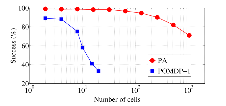
Figure 2: Ability to successfully achieve the assigned goal, as a function of the number of cells in the domain; with a limit on the time to compute policies PA significantly increases accuracy in comparison with just POMDP-1 as the number of cells in the domain increases.

Next, we computed the time taken by PA to generate a plan as the size of the domain increases. Domain size is characterized based on the number of rooms and the number of objects in the domain. We conducted three sets of experiments in which the robot reasons with: (1) all available knowledge of domain objects and rooms; (2) only knowledge relevant to the assigned goal—e.g., if the robot knows an object’s default location, it need not reason about other objects and rooms in the domain to locate this object; and (3) relevant knowledge and knowledge of an additional $20\%$ of randomly selected domain objects and rooms. Figure 3 summarizes these results. We observe that PA supports the generation of appropriate plans for domains with a large number of rooms and objects. We also observe that using only the knowledge relevant to the goal significantly reduces the planning time—such knowledge can be automatically selected using the relationships included in the HL system description. Furthermore, if we only use a probabilistic approach (POMDP-1), it soon becomes computationally intractable to generate a plan for domains with many objects and rooms; these results are not shown in Figure 3—see (?; ?).

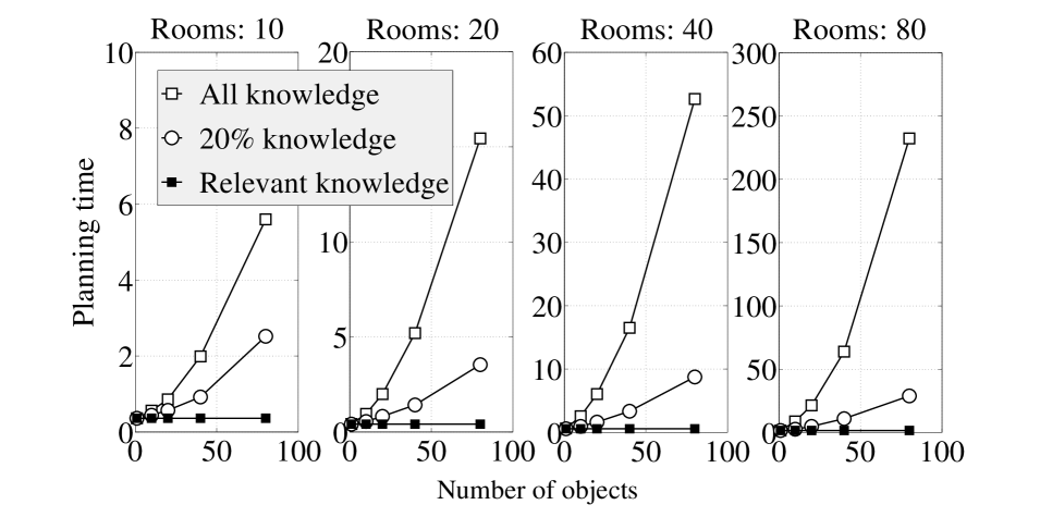
Figure 3: Planning time as a function of the number of rooms and the number of objects in the domain—$PA$ scales to larger number of rooms and objects.

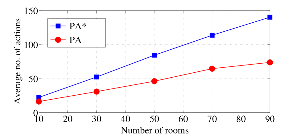
Figure 4: Effect of using default knowledge—principled representation of defaults significantly reduces the number of actions (and thus time) for achieving assigned goal.

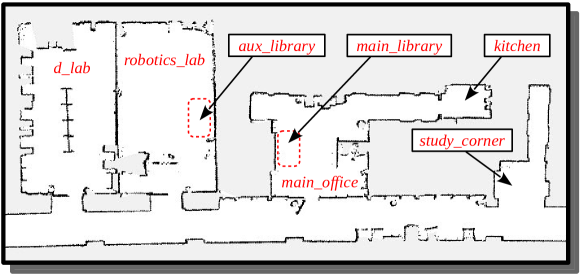
(a) Domain map

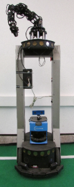
(b) Robot platform

Figure 5: Subset of the map of the second floor of our department; specific places are labeled as shown, and used during planning to achieve the assigned goals. The robot platform used in the experimental trials is also shown.

To evaluate H2, we first conducted multiple trials in which PA was compared with $PA^{*}$, a version that does not include any default knowledge. Figure 4 summarizes the average number of actions executed per trial as a function of the number of rooms in the domain—each sample point is the average of $10000$ trials. The goal in each trial is (as before) to move a specific object to a specific place. We observe that the principled use of default knowledge significantly reduces the number of actions (and thus time) required to achieve the assigned goal. Next PA was compared with POMDP-2, which assigns high probability values to default information and suitably revises the initial belief state. We observe that the effect of assigning a probability value to defaults is arbitrary depending on multiple factors: (a) the numerical value chosen; and (b) whether the ground truth matches the default information. For instance, if a large probability is assigned to the default knowledge that books are typically in the library, but the book the robot has to move is an exception to the default (e.g., a cookbook), it takes a significantly large amount of time for POMDP-2 to revise (and recover from) the initial belief. PA, on the other hand, enables the robot to revise initial defaults and encode exceptions to defaults.

Robot Experiments:

In addition to the trials in simulated domains, we compared PA with POMDP-1 on a wheeled robot over $50$ trials conducted on two floors of our department building. This domain includes places in addition to those included in our illustrative example, e.g., Figure 5(a) shows a subset of the domain map of the third floor of our department, and Figure 5(b) shows the wheeled robot platform. Such domain maps are learned by the robot using laser range finder data, and revised incrementally over time. Manipulation by physical robots is not a focus of this work. Therefore, once the robot is next to the desired object, it currently asks for the object to be placed in the extended gripper; future work will include existing probabilistic algorithms for manipulation in the LL.

For experimental trials on the third floor, we considered $15$ rooms, which includes faculty offices, research labs, common areas and a corridor. To make it feasible to use POMDP-1 in such large domains, we used our prior work on a hierarchical decomposition of POMDPs for visual sensing and information processing that supports automatic belief propagation across the levels of the hierarchy and model generation in each level of the hierarchy (?; ?). The experiments included paired trials, e.g., over $15$ trials (each), POMDP-1 takes $1.64$ as much time as PA (on average) to move specific objects to specific places. For these paired trials, this $39\%$ reduction in execution time provided by PA is statistically significant: p-value $=0.0023$ at the $95\%$ significance level.

Consider a trial in which the robot’s objective is to bring a specific textbook to the place named study_corner. The robot uses default knowledge to create an HL plan that causes the robot to move to and search for the textbook in the main_library. When the robot does not find this textbook in the main_library after searching using a suitable LL policy, replanning in the HL causes the robot to investigate the aux_library. The robot finds the desired textbook in the aux_library and moves it to the target location. A video of such an experimental trial can be viewed online:
http://youtu.be/8zL4R8te6wg

5 Conclusions

This paper described a knowledge representation and reasoning architecture for robots that integrates the complementary strengths of declarative programming and probabilistic graphical models. The system descriptions of the tightly coupled high-level (HL) and low-level (LL) domain representations are provided using an action language, and the HL definition of recorded history is expanded to allow prioritized defaults. Tentative plans created in the HL using defaults and commonsense reasoning are implemented in the LL using probabilistic algorithms, generating observations that add suitable statements to the HL history. In the context of robots moving objects to specific places in indoor domains, experimental results indicate that the architecture supports knowledge representation, non-monotonic logical inference and probabilistic planning with qualitative and quantitative descriptions of knowledge and uncertainty, and scales well as the domain becomes more complex. Future work will further explore the relationship between the HL and LL transition diagrams, and investigate a tighter coupling of declarative logic programming and probabilistic reasoning for robots.

References

- [Balai, Gelfond, and Zhang 2013] Balai, E.; Gelfond, M.; and Zhang, Y. 2013. Towards Answer Set Programming with Sorts. In International Conference on Logic Programming and Nonmonotonic Reasoning.
- [Balduccini and Gelfond 2003] Balduccini, M., and Gelfond, M. 2003. Logic Programs with Consistency-Restoring Rules. In Logical Formalization of Commonsense Reasoning, AAAI Spring Symposium Series, 9–18.
- [Baral, Gelfond, and Rushton 2009] Baral, C.; Gelfond, M.; and Rushton, N. 2009. Probabilistic Reasoning with Answer Sets. Theory and Practice of Logic Programming 9(1):57–144.
- [Baral 2003] Baral, C. 2003. Knowledge Representation, Reasoning and Declarative Problem Solving. Cambridge University Press.
- [Chen et al. 2012] Chen, X.; Xie, J.; Ji, J.; and Sui, Z. 2012. Toward Open Knowledge Enabling for Human-Robot Interaction. Journal of Human-Robot Interaction 1(2):100–117.
- [Erdem, Aker, and Patoglu 2012] Erdem, E.; Aker, E.; and Patoglu, V. 2012. Answer Set Programming for Collaborative Housekeeping Robotics: Representation, Reasoning, and Execution. Intelligent Service Robotics 5(4).
- [Gelfond and Kahl 2014] Gelfond, M., and Kahl, Y. 2014. Knowledge Representation, Reasoning and the Design of Intelligent Agents. Cambridge University Press.
- [Gelfond 2008] Gelfond, M. 2008. Answer Sets. In Frank van Harmelen and Vladimir Lifschitz and Bruce Porter., ed., Handbook of Knowledge Representation. Elsevier Science. 285–316.
- [Ghallab, Nau, and Traverso 2004] Ghallab, M.; Nau, D.; and Traverso, P. 2004. Automated Planning: Theory and Practice. San Francisco, USA: Morgan Kaufmann.
- [Halpern 2003] Halpern, J. 2003. Reasoning about Uncertainty. MIT Press.
- [Hanheide et al. 2011] Hanheide, M.; Gretton, C.; Dearden, R.; Hawes, N.; Wyatt, J.; Pronobis, A.; Aydemir, A.; Gobelbecker, M.; and Zender, H. 2011. Exploiting Probabilistic Knowledge under Uncertain Sensing for Efficient Robot Behaviour. In International Joint Conference on Artificial Intelligence.
- [Hoey et al. 2010] Hoey, J.; Poupart, P.; Bertoldi, A.; Craig, T.; Boutilier, C.; and Mihailidis, A. 2010. Automated Handwashing Assistance for Persons with Dementia using Video and a Partially Observable Markov Decision Process. Computer Vision and Image Understanding 114(5):503–519.
- [Kaelbling and Lozano-Perez 2013] Kaelbling, L., and Lozano-Perez, T. 2013. Integrated Task and Motion Planning in Belief Space. International Journal of Robotics Research 32(9-10).
- [Laird, Newell, and Rosenbloom 1987] Laird, J. E.; Newell, A.; and Rosenbloom, P. 1987. SOAR: An Architecture for General Intelligence. Artificial Intelligence 33(3).
- [Langley and Choi 2006] Langley, P., and Choi, D. 2006. An Unified Cognitive Architecture for Physical Agents. In The Twenty-first National Conference on Artificial Intelligence (AAAI).
- [Leone et al. 2006] Leone, N.; Pfeifer, G.; Faber, W.; Eiter, T.; Gottlob, G.; Perri, S.; and Scarcello, F. 2006. The DLV System for Knowledge Representation and Reasoning. ACM Transactions on Computational Logic 7(3):499–562.
- [Li and Sridharan 2013] Li, X., and Sridharan, M. 2013. Move and the Robot will Learn: Vision-based Autonomous Learning of Object Models. In International Conference on Advanced Robotics.
- [Milch et al. 2006] Milch, B.; Marthi, B.; Russell, S.; Sontag, D.; Ong, D. L.; and Kolobov, A. 2006. BLOG: Probabilistic Models with Unknown Objects. In Statistical Relational Learning. MIT Press.
- [Ong et al. 2010] Ong, S. C.; Png, S. W.; Hsu, D.; and Lee, W. S. 2010. Planning under Uncertainty for Robotic Tasks with Mixed Observability. International Journal of Robotics Research 29(8):1053–1068.
- [Richardson and Domingos 2006] Richardson, M., and Domingos, P. 2006. Markov Logic Networks. Machine learning 62(1).
- [Rosenthal and Veloso 2012] Rosenthal, S., and Veloso, M. 2012. Mobile Robot Planning to Seek Help with Spatially Situated Tasks. In National Conference on Artificial Intelligence.
- [Sanner and Kersting 2010] Sanner, S., and Kersting, K. 2010. Symbolic Dynamic Programming for First-order POMDPs. In National Conference on Artificial Intelligence (AAAI).
- [Somani et al. 2013] Somani, A.; Ye, N.; Hsu, D.; and Lee, W. S. 2013. DESPOT: Online POMDP Planning with Regularization. In Advances in Neural Information Processing Systems (NIPS).
- [Sridharan, Wyatt, and Dearden 2010] Sridharan, M.; Wyatt, J.; and Dearden, R. 2010. Planning to See: A Hierarchical Aprroach to Planning Visual Actions on a Robot using POMDPs. Artificial Intelligence 174:704–725.
- [Talamadupula et al. 2010] Talamadupula, K.; Benton, J.; Kambhampati, S.; Schermerhorn, P.; and Scheutz, M. 2010. Planning for Human-Robot Teaming in Open Worlds. ACM Transactions on Intelligent Systems and Technology 1(2):14:1–14:24.
- [Zhang, Sridharan, and Bao 2012] Zhang, S.; Sridharan, M.; and Bao, F. S. 2012. ASP+POMDP: Integrating Non-monotonic Logical Reasoning and Probabilistic Planning on Robots. In International Joint Conference on Development and Learning and on Epigenetic Robotics.
- [Zhang, Sridharan, and Washington 2013] Zhang, S.; Sridharan, M.; and Washington, C. 2013. Active Visual Planning for Mobile Robot Teams using Hierarchical POMDPs. IEEE Transactions on Robotics 29(4).