A unified approach to entanglement criteria using the Cauchy-Schwarz and Hölder inequalities

Abstract

We present unified approach to different recent entanglement criteria. Although they were developed in different ways, we show that they are all applications of a more general principle given by the Cauchy-Schwarz inequality. We explain this general principle and show how to derive with it not only already known but also new entanglement criteria. We systematically investigate its potential and limits to detect bipartite and multipartite entanglement.

I Introduction

The phenomenon of entanglement is of fundamental interest since it is a main difference between the classical and the quantum world. Furthermore, it is believed to be the central resource for quantum computing and protecting quantum communication. The existing entanglement criteria solve the problem of characterizing entanglement only for certain classes of states and, in addition, some of them are very resource intensive if applied experimentally. For example, to apply the famous positive-partial-transpose (PPT) criterion Peres (1996); Horodecki et al. (1996) experimentally, a full quantum state tomography is necessary in practice. Some other entanglement criteria are formulated as inequalities for mean values of observables Shchukin and Vogel (2005); Hillery and Zubairy (2006); Gühne and Seevinck (2010); Hillery et al. (2010); Dür and Cirac (2000); Huber et al. (2010). This sort of entanglement criteria are especially useful to detect entanglement in experiments since complete knowledge about the quantum state is not necessary.

When going from bipartite entanglement to multipartite entanglement, the detection and characterization of entanglement become even more complicated. First of all, there exist different degrees of entanglement. That is, an $N$-partite entangled state $\varrho$ may be a convex combination of pure entangled states with maximally $k$ entangled parties. If at least one $N$-partite entangled pure state is necessary to form $\varrho$, we call the state genuine multipartite entangled. Since the representation of a mixed state by a convex sum of pure states is not unique, the entanglement characterization of multipartite states is more than the combination of bipartite entanglement criteria. For example, there exist states which are entangled under every bipartite split but are not genuine multipartite entangled. On the other hand, there exist states, which are separable under every possible bipartite split, but not fully separable.

Consequently, there are many different criteria and there are many different ways to develop them. To give an example, Hillery and Zubairy developed in Ref. Hillery and Zubairy (2006) first a criterion based on uncertainties, followed by a generalized entanglement criterion solely based on the Cauchy-Schwarz inequality and the properties of separable states. Whereas this approach used only a single operator per subsystems, we gain more freedom by using two operators per subsystem. In this way, we develop in this paper a general principle to create entanglement criteria. Many already existing criteria follow immediately from this new principle, but also new criteria can be created.

This paper consists of two main parts: In Sec. II we introduce our scheme of developing entanglement criteria with the help of the Cauchy-Schwarz inequality. Here, we will first concentrate on bipartite entanglement in Sec. II.1. We explain the intimate connection of the PPT criterion Peres (1996); Horodecki et al. (1996) to our criterion and give explicit examples of classes of states which can and which can not be detected by our criterion. Afterwards, in Sec. II.2, we generalize our scheme to multipartite entanglement by using the Hölder inequality and show that in the multipartite case our criterion can detect entangled states which cannot be detected by the PPT criterion. In Sec. III we discuss several already existing criteria and demonstrate how they can be derived within our scheme. In this way, a connection between the different criteria are pointed out and the advantages and disadvantages of the different criteria become visible.

II Entanglement criteria from the Cauchy-Schwarz inequality

First, recall that a two-particle state $\varrho$ is separable, if it can be written as a mixture of product states

$$\varrho=\sum_{k}p_{k}\varrho_{k}^{A}\otimes\varrho_{k}^{B},$$ (1)

where the $p_{k}$ form a probability distribution. We aim at deriving entanglement criteria in the form of inequalities which hold for separable states, but which can be violated by entangled states. Our main tool are two simple facts:
(i) we use the property of product states $\varrho=\varrho^{A}\otimes\varrho^{B}$ that

$$\langle AB\rangle_{\rm ps}=\langle{A}\rangle_{\varrho^{A}}\langle{B}\rangle_{\varrho^{B}}$$ (2)

for operators $A$ and $B$ acting on Alice’s and Bobs subsystem, respectively. Here and in the following, $\langle{\dots}\rangle_{\rm ps}$ denotes that the expectation value is taken for a product state. Similarly $\langle{\dots}\rangle_{\rm sep}$ denotes an expectation value for a separable state.
(ii) The Cauchy Schwarz (CS) inequality Cauchy (1821)

$$|\langle x,y\rangle|^{2}\leq\langle x,x\rangle\langle y,y\rangle$$ (3)

where $x$ and $y$ are two vectors and $\langle\cdot,\cdot\rangle$ defines an inner product.

II.1 Bipartite entanglement

We concentrate on expectation values of a bipartite system which can be written as $\langle A_{1}A_{2}B_{1}B_{2}\rangle$ where the operators $A_{i}$ and $B_{j}$ acting on Alice’s and Bob’s subsystem, respectively. For a pure state, these expectation values can be interpreted as the inner product of the two vectors $|\psi_{1}\rangle\equiv A_{1}^{\dagger}B_{1}^{\dagger}|\psi\rangle$ and $|\psi_{2}\rangle\equiv A_{2}B_{2}|\psi\rangle$. Since the scalar product is bilinear, all fragmentation of a scaler product into a bra- and a ket-vector can be described by two operators per subsystems. More than two are not necessary, since they can be always combined to a single operator acting on the bra- and one acting on the ket-vector. The expectation value $\langle A_{1}A_{2}B_{1}B_{2}\rangle$ can be used to detect entanglement by using the following theorem:

Theorem II.1

The inequality

$$|\langle A_{1}A_{2}B_{1}B_{2}\rangle_{\mkern 1.0mu\mathrm{sep}\mkern 1.0mu}|^{2}\leq\langle A_{1}A_{1}^{\dagger}B_{2}^{\dagger}B_{2}\rangle_{\mkern 1.0mu\mathrm{sep}\mkern 1.0mu}\langle A_{2}^{\dagger}A_{2}B_{1}B_{1}^{\dagger}\rangle_{\mkern 1.0mu\mathrm{sep}\mkern 1.0mu}.$$ (4)

is valid for separable states and can only be violated by entangled states.

• For product states $|\phi\rangle=|a\rangle|b\rangle=|a,b\rangle$, we can write the expectation value as the product of the expectation values of the subsystems. By applying the CS inequality to every single subsystem we get

  $$|\langle a,b|A_{1}A_{2}B_{1}B_{2}|a,b\rangle|^{2} = |\langle a|A_{1}A_{2}|a\rangle|^{2}|\langle b|B_{1}B_{2}|b\rangle|^{2}$$ (5)

  $$\leq \langle a|A_{1}A_{1}^{\dagger}|a\rangle\langle a|A_{2}^{\dagger}A_{2}|a\rangle$$

  $$\times\langle b|B_{1}B_{1}^{\dagger}|b\rangle\langle b|B_{2}^{\dagger}B_{2}|b\rangle$$

  which is equal to

  $$|\langle A_{1}A_{2}B_{1}B_{2}\rangle_{\mkern 1.0mu\mathrm{ps}\mkern 1.0mu}|^{2}\leq\langle A_{1}A_{1}^{\dagger}B_{2}^{\dagger}B_{2}\rangle_{\mkern 1.0mu\mathrm{ps}\mkern 1.0mu}\langle A_{2}^{\dagger}A_{2}B_{1}B_{1}^{\dagger}\rangle_{\mkern 1.0mu\mathrm{ps}\mkern 1.0mu}.$$ (6)

  In order to see that this inequality holds also for mixed states, note first that the root of the left-hand side $|\langle A_{1}A_{2}B_{1}B_{2}\rangle_{\mkern 1.0mu\mathrm{ps}\mkern 1.0mu}|$ is convex in the state, while the root of the right-hand side is of the type $\sqrt{f(\varrho)g(\varrho)}$, where $f$ and $g$ are positive functions. This implies that it is concave Gühne and Seevinck (2010). Therefore, this inequality is also valid for mixtures of product states which proves the correctness of Eq. (4) for any separable state.

  $\square$

With the help of the CS inequality we derive for general states

$$|\langle A_{1}A_{2}B_{1}B_{2}\rangle|^{2}\leq\langle A_{1}A_{1}^{\dagger}B_{1}B_{1}^{\dagger}\rangle\langle A_{2}^{\dagger}A_{2}B_{2}^{\dagger}B_{2}\rangle,$$ (7)

which provides a tight upper limit for all states.

Depending on the choice of the operators $A_{j}$ and $B_{j}$ the inequality Eq. (4) may provide a stricter limit than Eq. (7). If yes, then there exist states which violates Eq. (4). These states must be entangled and therefore Eq. (4) is able to detect entanglement.

Regarding the application of Theorem II.1 we note: (i) The ability of Eq. (4) to detect entanglement depends on the chosen operators $A_{j}$ and $B_{j}$. For example, by a comparison of Eq. (7) and Eq. (4) we immediately find that if $A_{1}A_{1}^{\dagger}=A_{2}^{\dagger}A_{2}$ or $B_{1}B_{1}^{\dagger}=B_{2}^{\dagger}B_{2}$ Eq. (4) cannot be violated for any state. (ii) The optimal choice of the operators $A_{j}$ and $B_{j}$ depends in general on the state $\varrho$. (iii) Whereas Eq. (4) is valid for general mixed separable states, Eq. (5) used to develop Eq. (4) is only valid for pure product states. As a consequence, great care concerning convexity has to be taken when generalizing Eq. (4) to multipartite systems.

After the development of the entanglement criteria Eq. (4) we will investigate the bipartite case now in more detail. First, we discuss the best choice of operators.

Theorem II.2

The best choice of the operators $A_{j}$ are given by

$$A_{1}=|a\rangle\langle\varphi|;\;A_{2}=|\varphi\rangle\langle\alpha|$$ (8)

with $|a\rangle$, $|\alpha\rangle$ and $|\varphi\rangle$ being pure states of Alice’s subsystem, and an analogous choice for Bob.

• Any pair of operators $A_{1}$ and $A_{2}$ can be written as

  $$A_{1} = \sum\limits_{j}x_{j}|a_{j}\rangle\langle\varphi_{j}|$$ (9)

  $$A_{2} = \sum\limits_{j}y_{j}|\varphi_{j}\rangle\langle\alpha_{j}|$$ (10)

  with $\{|\varphi_{j}\rangle\}$ being an orthonormal basis of Alice’s subsystem. As a consequence, the entanglement criterion Eq. (4) turns into

  $$\Big{|}\sum\limits_{j}x_{j}y_{j}\text{Tr\,}[|a_{j}\rangle_{A}\langle\alpha_{j}|B_{1}B_{2}\varrho]\Big{|}^{2}\leq\sum\limits_{j}|x_{j}|^{2}p_{j}\sum\limits_{k}|y_{k}|^{2}q_{k}$$ (11)

  where we defined

  $$p_{j} \equiv \text{Tr\,}[|a_{j}\rangle\langle a_{j}|B_{2}^{\dagger}B_{2}\varrho],$$

  $$q_{k} \equiv \text{Tr\,}[|\alpha_{k}\rangle\langle\alpha_{k}|B_{1}B_{1}^{\dagger}\varrho].$$ (12)

  The right hand side of this equation is equal to

  $$\begin{split}RS1=&\sum\limits_{j}|x_{j}|^{2}|y_{j}|^{2}p_{j}q_{j}\\ &+\sum\limits_{j}\sum\limits_{k>j}|x_{j}|^{2}|y_{k}|^{2}p_{j}q_{k}+|x_{k}|^{2}|y_{j}|^{2}p_{k}q_{j}\end{split}$$ (13)

  On the other hand, we can estimate the left hand side by

  $$\begin{split}&\Big{|}\sum\limits_{j}x_{j}y_{j}\text{Tr\,}[|a_{j}\rangle\langle\alpha_{j}|B_{1}B_{2}\varrho]\Big{|}^{2}\\ &\leq\Big{(}\sum\limits_{j}|x_{j}||y_{j}|\left|\text{Tr\,}[|a_{j}\rangle_{A}\langle\alpha_{j}|B_{1}B_{2}\varrho]\right|\Big{)}^{2}\end{split}$$ (14)

  and use Eq. (4) for every single term in the summation. This leads to

  $$\Big{|}\sum\limits_{j}x_{j}y_{j}\text{Tr\,}[|a_{j}\rangle\langle\alpha_{j}|B_{1}B_{2}\varrho]\Big{|}^{2}\leq\Big{(}\sum\limits_{j}|x_{j}||y_{j}|\sqrt{p_{j}q_{j}}\Big{)}^{2}$$ (15)

  By expanding the right hand side we get

  $$\begin{split}RS2=&\sum\limits_{j}|x_{j}|^{2}|y_{j}|^{2}p_{j}q_{j}\\ &+\sum\limits_{j}\sum\limits_{k>j}2|x_{j}x_{k}y_{j}y_{k}|\sqrt{p_{j}p_{k}q_{j}q_{k}}\end{split}$$ (16)

  By using $r^{2}+s^{2}\geq 2rs$ valid for all real numbers $r,s$ and identifying

  $$r = |x_{j}||y_{k}|\sqrt{p_{j}q_{k}}$$ (17)

  $$s = |x_{k}||y_{j}|\sqrt{p_{k}q_{j}}$$ (18)

  for all arbitrary but fixed combination of $j$ and $k$ we find by comparing Eq. (13) with Eq. (16)

  $$RS2\leq RS1.$$ (19)

  As a consequence, using several entanglement criteria with operators

  $$A_{1}=|a_{j}\rangle\langle\varphi_{j}|;\;A_{2}=|\varphi_{j}\rangle\langle\alpha_{j}|$$ (20)

  for every $j$ separately leads to a stronger criterion than a linear combination of these operators.     $\square$

Naturally the same holds for Bob’s subsystems which leads to the well known entanglement criterion Gühne and Seevinck (2010); Huber et al. (2010)

$$\left|\langle\alpha,\beta|\varrho|a,b\rangle_{\mkern 1.0mu\mathrm{sep}\mkern 1.0mu}\right|\leq\sqrt{\langle a,\beta|\varrho|a,\beta\rangle_{\mkern 1.0mu\mathrm{sep}\mkern 1.0mu}\langle\alpha,b|\varrho|\alpha,b\rangle_{\mkern 1.0mu\mathrm{sep}\mkern 1.0mu}}.$$ (21)

Now, we turn to the question which states can be detected by Theorem II.1. Similar to the criterion from Hillery and Zubairy Hillery et al. (2009), our criterion is strongly connected to the positive partial transpose (PPT) criterion in the bipartite case Peres (1996); Horodecki et al. (1996).

Theorem II.3

The criterion Theorem II.1 for detecting bipartite entanglement detects only states with a negative partial transpose (NPT).

• By using the partial transpose with respect to system A (written as $T_{A}$) acting on the state $\varrho$ as well as on the operators $A_{1}$ and $A_{2}$ we rewrite the expectation value

  $$|\langle A_{1}A_{2}B_{1}B_{2}\rangle|=\left|\text{Tr\,}[A_{2}^{T}A_{1}^{T}B_{1}B_{2}\varrho^{T_{A}}]\right|.$$ (22)

  If $\varrho$ is PPT, than $\varrho^{T_{A}}$ is a valid density operator and the Cauchy-Schwarz inequality for expectation values

  $$\left|\text{Tr\,}[OP\varrho]\right|\leq\sqrt{\text{Tr\,}[OO^{\dagger}\varrho]\text{Tr\,}[P^{\dagger}P\varrho]}$$ (23)

  can be applied. This leads to

  $$\begin{split}\left|\text{Tr\,}[A_{2}^{T}A_{1}^{T}B_{1}B_{2}\varrho_{\mkern 1.0mu\mathrm{PPT}\mkern 1.0mu}^{T_{A}}]\right|\leq&\sqrt{\text{Tr\,}[A_{2}^{T}\left(A_{2}^{T}\right)^{\dagger}B_{1}B_{1}^{\dagger}\varrho_{\mkern 1.0mu\mathrm{PPT}\mkern 1.0mu}^{T_{A}}]}\\ &\times\sqrt{\text{Tr\,}[\left(A_{1}^{T}\right)^{\dagger}A_{1}^{T}B_{2}^{\dagger}B_{2}\varrho_{\mkern 1.0mu\mathrm{PPT}\mkern 1.0mu}^{T_{A}}]}\end{split}$$ (24)

  were we identified $O=A_{2}^{T}B_{1}$ and $P=A_{1}^{T}B_{2}$. Writing the expectation value again with respect to $\varrho$ we finally arrive at

  $$\begin{split}|\langle A_{1}A_{2}B_{1}B_{2}\rangle_{\mkern 1.0mu\mathrm{PPT}\mkern 1.0mu}|\leq&\sqrt{\langle A_{2}^{\dagger}A_{2}B_{1}B_{1}^{\dagger}\rangle_{\mkern 1.0mu\mathrm{PPT}\mkern 1.0mu}\langle A_{1}A_{1}^{\dagger}B_{2}^{\dagger}B_{2}\rangle_{\mkern 1.0mu\mathrm{PPT}\mkern 1.0mu}}\end{split}$$ (25)

  which is equal to Eq. (4). As a consequence, PPT states are not able to violate Eq. (4).     $\square$

We note that Theorem II.3 is only valid for the bipartite case. In the multipartite case, also PPT-states can be detected, since our criteria not only checks bipartite entanglement but real multipartite entanglement as we will show in the next section. However, we will once again stay in the bipartite case and identify now a few classes of entangled states which can be detected by Eq. (4). Furthermore, we will also show how to find the right operators $A_{j}$ and $B_{j}$ for these cases. To achieve this task, the following lemma will be helpful:

Lemma II.4

Let $|\lambda_{j}^{+}\rangle$ be the eigenstates of $\varrho^{T_{A}}$ corresponding to the positive eigenvalues and $|\lambda_{j}^{-}\rangle$ the ones corresponding to negative eigenvalues. Furthermore, we assume that there exist states $\{|a_{k}\rangle\}$ and $\{|b_{k}\rangle\}$ of Alice’s and Bobs subsystems, respectively, with $k\in\{1,2\}$ such that

$$\langle a_{2},b_{1}|\lambda_{j}^{+}\rangle = c^{+}\langle a_{1},b_{2}|\lambda_{j}^{+}\rangle$$ (26)

$$\langle a_{2},b_{1}|\lambda_{j}^{-}\rangle = c^{-}\langle a_{1},b_{2}|\lambda_{j}^{-}\rangle$$ (27)

with $c^{\pm}$ independent of $j$ and $c^{+}c^{-}<0$. By choosing the operators

$$A_{1}=|a_{1}^{\ast}\rangle\langle\alpha| B_{1}=|b_{1}\rangle\langle\beta|$$ (28)

$$A_{2}=|\alpha\rangle\langle a_{2}^{\ast}| B_{2}=|\beta\rangle\langle b_{2}|$$ (29)

with $|\alpha\rangle,|\beta\rangle$ being arbitrary states of Alice’s and Bobs subsystems, respectively, Eq. (4) is violated by the state $\varrho$.

• Although the state under consideration is not PPT, we can use some calculations from the proof of Theorem II.3. By defining $p_{j}=\langle a_{1},b_{2}|\lambda_{j}^{+}\rangle$ and $q_{j}=\langle a_{1},b_{2}|\lambda_{j}^{-}\rangle$ we obtain for the left hand side of Eq. (24)

  $$LS \equiv \left|\langle a_{1},b_{2}|\varrho^{T_{A}}|a_{2},b_{1}\rangle\right|$$ (30)

  $$= |c^{+}|\sum_{j}\lambda_{j}^{+}|p_{j}|^{2}+|c^{-}|\sum_{j}|\lambda_{j}^{-}||q_{j}|^{2}.$$ (31)

  The right hand side becomes

  $$RS \equiv \sqrt{\langle a_{2},b_{1}|\varrho|a_{2},b_{1}\rangle\langle a_{1},b_{2}|\varrho|a_{1},b_{2}\rangle}$$

  $$= \sqrt{|c^{+}|^{2}\sum_{j}\lambda_{j}^{+}|p_{j}|^{2}-|c^{-}|^{2}\sum_{j}|\lambda_{j}^{-}||q_{j}|^{2}}$$

  $$\times \sqrt{\sum_{j}\lambda_{j}^{+}|p_{j}|^{2}-\sum_{j}|\lambda_{j}^{-}||q_{j}|^{2}}.$$ (33)

  By expanding the product we arrive at

  $$\begin{split}RS=&\Big{[}|c^{+}|^{2}\Big{(}\sum_{j}\lambda_{j}^{+}|p_{j}|^{2}\Big{)}^{2}+|c^{-}|^{2}\Big{(}\sum_{j}|\lambda_{j}^{-}||q_{j}|^{2}\Big{)}^{2}\\ &-\left(|c^{+}|^{2}+|c^{-}|^{2}\right)\Big{(}\sum_{j}\lambda_{j}^{+}|p_{j}|^{2}\Big{)}\Big{(}\sum_{j}|\lambda_{j}^{-}||q_{j}|^{2}\Big{)}\Big{]}^{1/2}.\end{split}$$ (34)

  With the help of $-\left(|c^{+}|^{2}+|c^{-}|^{2}\right)\leq-2|c^{+}||c^{-}|$ we are able to estimate the right side by

  $$RS\leq\Big{|}|c^{+}|\sum_{j}\lambda_{j}|p_{j}|^{2}-|c^{-}|\sum_{j}|\lambda_{j}^{-}||q_{j}|^{2}\Big{|}.$$ (35)

  A comparison of Eq. (31) and Eq. (35) shows that the left hand side of Eq. (24) is the summation of two positive numbers whereas the right side is smaller or equal than the absolute value of the difference of the same two positive numbers. As a consequence, we have $LS>RS$ and a violation of Eq. (24) which implies a violation of criterion Theorem II.1.     $\square$

Now, we are able to identify certain classes of entangled states that can be detected with our criterion. One of these classes are bipartite qubits states:

Theorem II.5

Every entangled two-qubit state $\varrho$ can be detected with Theorem II.1

• Every entangled two-qubit state is an NPT-state. All eigenstates $|\lambda_{j}^{-}\rangle$ corresponding to a negative eigenvalue $\lambda_{j}^{-}$ of the partial transpose of $\varrho$ form an entangled subspace Johnston (2013); Rana (2013). That means it is not possible to construct a product state by a superposition of $|\lambda_{j}^{-}\rangle$. As a consequence, for two-qubit states only one single negative eigenvalue can exist Sanpera et al. (1998). Its eigenstate is given in its Schmidt basis by

  $$|\lambda^{-}\rangle\equiv s_{0}|00\rangle+s_{1}|11\rangle.$$ (36)

  with $s_{j}>0$. Since a two-qubit state is separable iff the determinant of its partial transpose is nonnegative Augusiak et al. (2008), $\varrho^{T}_{A}$ has three strictly positive eigenvalues $\lambda^{+}_{j}>0$. Their corresponding eigenstates are given by

  $$|\lambda_{k}^{+}\rangle\equiv r_{k}\left(s_{1}|00\rangle-s_{0}|11\rangle\right)+\gamma_{k}|01\rangle+\delta_{k}|10\rangle$$ (37)

  with arbitrary coefficients $r_{k}$, $\gamma_{k}$ and $\delta_{k}$ and at least one $k$ for which $r_{k}\neq 0$. By choosing the states $|a_{2},b_{1}\rangle=|00\rangle$ and $|a_{2},b_{1}\rangle=|11\rangle$ we find

  $$\langle 00|\lambda_{k}^{+}\rangle=r_{k}s_{1}\,,\,\langle 11|\lambda_{k}^{+}\rangle=-r_{k}s_{0}.$$ (38)

  Therefore the constant $c^{+}$ defined in Lemma II.4 does exist for these states and is given by $c^{+}=-s_{1}/s_{0}$. Similar we find $c^{-}=s_{0}/s_{1}$ and as a consequence Lemma II.4 can be applied.      $\square$

We want to stress out the fact that $\varrho$ is entangled iff the determinant of $\varrho^{T}_{A}$ is negative is not necessary for our proof. Moreover, the existence of at least one $r_{k}\neq 0$ can be proven from our previous considerations:

Assume that there were an NPT two-qubit state with a vanishing eigenvalue, such that $r_{k}=0$ for all $k$. Since the trace is preserved under partial transposition, there must exist at least one positive eigenvalue and therefore there is some $\gamma_{k}\neq 0$ or $\delta_{k}\neq 0$. Let us assume $\gamma_{k_{0}}\neq 0$. It follows that we can choose the product states $|a_{2},b_{1}\rangle=|00\rangle+|01\rangle$ and $|a_{1},b_{2}\rangle=|00\rangle-|01\rangle$ and find

$$\langle a_{2}b_{1}|\lambda_{k}^{+}\rangle=\gamma_{k}\,,\,\langle a_{1},b_{2}|\lambda_{k}^{+}\rangle=-\gamma_{k}.$$ (39)

Therefore, the constant $c^{+}$ is given by $c^{+}=-1$ and similar $c^{-}=1$. By using Lemma II.4 we get a violation of Eq. (24). However, in this case we would have $A_{1}A_{1}^{\dagger}=|0\rangle\langle 0|=A_{2}^{\dagger}A_{2}$ and for these operators Eq. (4) can never be violated. As a consequence if $|\lambda_{j}^{-}\rangle\equiv\alpha|00\rangle+\beta|11\rangle$ is an eigenvector of $\varrho^{T_{A}}$ with a negative eigenvalue then there must be an eigenvector $|\lambda_{j}^{+}\rangle$ with

$$\langle\lambda_{j}^{+}|\left(s_{1}|00\rangle-s_{0}|11\rangle\right)\neq 0.$$ (40)

Also in higher dimensions there exist classes of entangled states which can be detected with our criterion. One of these classes are entangled states mixed with with noise:

Theorem II.6

Every NPT-state of the form

$$\varrho_{\text{wn}}=p|\psi_{\text{ent}}\rangle\langle\psi_{\text{ent}}|+\frac{1-p}{D}\mathbbm{1}_{D},$$ (41)

with $\mathbbm{1}_{D}$ being the identity matrix of dimension $D$ of $\varrho$ and $|\psi_{\text{ent}}\rangle$ being a pure entangled state, can be detected by Eq. (4).

To prove this theorem, we use the following fact, that can be proved by direct calculation:

Lemma II.7

The partially transposed state $\varrho_{\text{wn}}^{T_{A}}$ with $|\psi_{\text{ent}}\rangle$ given in its Schmidt basis by $|\psi_{\text{ent}}\rangle=\sum_{j}s_{j}|jj\rangle$ has the following eigenvalues and eigenstates:

$$|\lambda_{j,j}\rangle=|j,j\rangle \lambda_{j,j}=\frac{1-p}{D}+ps_{j}^{2}$$ , (42)

$$|\lambda_{j,k}\rangle=\frac{|j,k\rangle\pm|k,j\rangle}{\sqrt{2}} \lambda_{j,k}=\frac{1-p}{D}\pm ps_{j}s_{k}$$ , (43)

Now we are able to prove the theorem:

• From the previous Lemma one finds that an eigenstate corresponding to negative eigenvalues is of the form

  $$|\lambda_{-}\rangle=\frac{|j_{0},k_{0}\rangle-|k_{0},j_{0}\rangle}{\sqrt{2}}$$ (44)

  and that

  $$|\lambda_{+}\rangle=\frac{|j_{0},k_{0}\rangle+|k_{0},j_{0}\rangle}{\sqrt{2}}$$ (45)

  is an eigenstate corresponding to a positive eigenvalue. Furthermore, $\langle j_{0},k_{0}|\lambda_{n}\rangle=\langle k_{0},j_{0}|\lambda_{n}\rangle=0$ for all other eigenstates $|\lambda_{n}\rangle$. By choosing $|a_{2},b_{1}\rangle=|j_{0},k_{0}\rangle$ and $|a_{1},b_{2}\rangle=|k_{0},j_{0}\rangle$ we find

  $$\langle a_{2},b_{1}|\lambda_{-}\rangle = -\langle a_{1},b_{2}|\lambda_{-}\rangle$$ (46)

  $$\langle a_{2},b_{1}|\lambda_{+}\rangle = +\langle a_{1},b_{2}|\lambda_{+}\rangle$$ (47)

  $$\langle a_{2},b_{1}|\lambda_{n}\rangle = \pm\langle a_{1},b_{2}|\lambda_{n}\rangle=0.$$ (48)

  As a consequence the constants $c^{+}$ and $c^{-}$ of Lemma II.4 do exist and therefore the entanglement of $\varrho_{\text{wn}}^{\text{PT}}$ can be detect with the help of Theorem II.1.     $\square$

It is important to point out a consequence of the optimality of choosing $A_{1/2}$ and $B_{1/2}$ such that the criterion takes the form of eq. (21). There are only up to four independent vectors (in the previous notation $|a\rangle,|b\rangle,|\alpha\rangle,|\beta\rangle$) appearing in the inequality. If we denote $|\alpha\rangle=\lambda|a\rangle+\sqrt{1-|\lambda|^{2}}|a^{\perp}\rangle$ with $\lambda=\langle a|\alpha\rangle$ it becomes obvious that the criterion is invariant under prior projection into the qubit subspace on Alice’s side given by $\mathbbm{1}_{2}=|a\rangle\langle a|+|a^{\perp}\rangle\langle a^{\perp}|$. As the same holds for Bob’s side we can conclude that the bipartite version of this theorem is actually equivalent to detecting entanglement in a $2\times 2$ dimensional subspace. From Ref. Horodecki et al. (1998) it follows that any violation of the criterion implies one-copy distillability, which on the other hand implies the impossibility of detecting some NPT states, such as the well known Werner state Werner (1989). In fact it also implies that we can strictly improve the detection strength of the criterion by applying it on multiple copies of the state, as there are known examples of states that are two-, but not one-copy distillable. However some NPT states are most likely beyond the reach of our criterion as e.g. the Werner state is conjectured to be NPT bound entangled, i.e. even up to infinitely many copies do not have an entangled $2\times 2$ subspace for a specific region of parameters.
A natural extension of our theorem that would close this (small) gap for bipartite systems is an extension to $D\times D$-dimensional subspaces, which could be written as

$$\text{Det}\begin{pmatrix}\rho_{i_{1}i_{1}i_{1}i_{1}}&\rho_{i_{1}i_{2}i_{2}i_{1}}&\cdots&\rho_{i_{1}i_{D}i_{D}i_{1}}\\ \rho_{i_{2}i_{1}i_{1}i_{2}}&\rho_{i_{2}i_{2}i_{1}i_{2}}&\cdots&\vdots\\ \vdots&\vdots&\ddots&\vdots\\ \rho_{i_{D}i_{1}i_{1}i_{D}}&\cdots&\cdots&\rho_{i_{D}i_{D}i_{D}i_{D}}\end{pmatrix}\geq 0\,,$$ (49)

with the notation $\langle ab|\rho_{PPT}|\alpha\beta\rangle=\rho_{ab\alpha\beta}$. This criterion is a natural extension of our main theorem to higher dimensions and in this form is in principle capable of detecting all NPT states, not only one-copy distillable ones. The caveat here is however, that due to the non-convex structure we can neither make use of the Cauchy-Schwarz inequality, nor find an analogue extension to the more interesting case of many particles. So instead we focus on our main theorem, which allows for a straightforward generalization to multipartite systems.

II.2 Multiparticle entanglement

Pure product states and mixed product states of the form $\varrho=\bigotimes_{j=1}^{N}\varrho_{j}$ with $\varrho_{j}$ do not contain any correlations (nc). The generalization of Eq. (5) to multipartite systems for these states is straightforward:

$$|\langle\bigotimes\limits_{k=1}^{N}P_{k}Q_{k}\rangle_{\mkern 1.0mu\mathrm{nc}\mkern 1.0mu}|\leq\prod\limits_{k=1}^{N}\sqrt{\langle P_{k}P_{k}^{\dagger}\rangle_{\mkern 1.0mu\mathrm{nc}\mkern 1.0mu}\langle Q_{k}^{\dagger}Q_{k}\rangle_{\mkern 1.0mu\mathrm{nc}\mkern 1.0mu}}$$ (50)

with operators $P_{k}$ and $Q_{k}$ acting on subsystem $k$. Again, we can combine expectation values of different subsystems and arrive at a generalization of Theorem II.1:

$$|\langle\bigotimes\limits_{k=1}^{N}P_{k}Q_{k}\rangle_{\mkern 1.0mu\mathrm{nc}\mkern 1.0mu}|\leq\prod\limits_{k=1}^{N}\sqrt{\langle P_{k}P_{k}^{\dagger}Q_{k+1}^{\dagger}Q_{k+1}\rangle}_{\mkern 1.0mu\mathrm{nc}\mkern 1.0mu}.$$ (51)

where we defined $Q_{N+1}=Q_{1}$. Also other combination of expectation values are possible. However, these inequalities are not convex and therefore in general not valid for mixed separable states.

To generalize entanglement criteria of the form of Eq. (51) to mixed fully separable states, we have to use the Hölder inequality. We will explain the generalization using the example of Eq. (51) for a tripartite state with the operators $A_{j}$, $B_{j}$ and $C_{j}$ acting on Alice’s, Bob’s and Charlie’s subsystem, respectively.

II.2.1 Scheme to develop entanglement criteria

Performing the following steps will result in an inequality to detect entanglement. We assume that we start with an fully separable state

$$\varrho=\sum_{j}p_{j}|\psi^{\mkern 1.0mu\mathrm{ps}\mkern 1.0mu}_{j}\rangle\!\langle\psi^{\mkern 1.0mu\mathrm{ps}\mkern 1.0mu}_{j}|$$ (52)

where the $|\psi^{\mkern 1.0mu\mathrm{ps}\mkern 1.0mu}_{j}\rangle$ are pure multiparticle product states as above.

• Write the expectation value $\langle A_{1}A_{2}B_{1}B_{2}C_{1}C_{2}\rangle$ of the fully seperable state as a convex combination of expectation values for pure product states $|\psi^{\mkern 1.0mu\mathrm{ps}\mkern 1.0mu}_{j}\rangle$.

  $$\langle A_{1}A_{2}B_{1}B_{2}C_{1}C_{2}\rangle_{\text{sep}}=\sum\limits_{j}p_{j}\langle A_{1}A_{2}B_{1}B_{2}C_{1}C_{2}\rangle_{{\mkern 1.0mu\mathrm{ps}\mkern 1.0mu},j}$$ (53)

  with $\sum_{j}p_{j}=1$ and $\langle\cdots\rangle_{{\mkern 1.0mu\mathrm{ps}\mkern 1.0mu},j}$ denoting the expectation value of state $|\psi^{\mkern 1.0mu\mathrm{ps}\mkern 1.0mu}_{j}\rangle$.

• Write every expectation value $\langle\cdots\rangle_{{\mkern 1.0mu\mathrm{ps}\mkern 1.0mu},j}$ as expectation values of single subsystems and apply the Cauchy Schwarz inequality to each of them

  $$|\langle A_{1}A_{2}B_{1}B_{2}C_{1}C_{2}\rangle_{\mkern 1.0mu\mathrm{sep}\mkern 1.0mu}|\leq\sum\limits_{j}p_{j}\sqrt{\langle A_{1}A_{1}^{\dagger}\rangle_{j}\langle A_{2}^{\dagger}A_{2}\rangle_{j}\cdots}.$$ (54)

  Since operators of the form $O=DD^{\dagger}$ are positive operators, it is also possible to increase the number of expectation values by using $\langle O\rangle=\sqrt[n]{\langle O\rangle^{n}}$ .

• Combine arbitrary expectation values of different subsystems, for example

  $$\begin{split}&|\langle A_{1}A_{2}B_{1}B_{2}C_{1}C_{2}\rangle_{\mkern 1.0mu\mathrm{sep}\mkern 1.0mu}|\\ \leq&\sum\limits_{j}p_{j}\sqrt{\langle A_{1}A_{1}^{\dagger}B_{2}^{\dagger}B_{2}\rangle_{j}\langle B_{1}B_{1}^{\dagger}C_{2}^{\dagger}C_{2}\rangle_{j}\langle C_{1}C_{1}^{\dagger}A_{2}^{\dagger}A_{2}\rangle_{j}}\end{split}$$ (55)

  It is also possible to combine more than two subsystems in a single expectation value.

• Use the generalized Hölder inequality Hardy et al. (1934)

  $$\sum\limits_{j}p_{j}x_{j}y_{j}\leq\Big{(}\sum\limits_{j}p_{j}x_{j}^{1/r}\Big{)}^{r}\Big{(}\sum\limits_{j}p_{j}y_{j}^{1/s}\Big{)}^{s}$$ (56)

  with $r+s=1$ and $p_{j}\geq 0$ to separate the summation of each expectation value. Here, the Hölder inequality may be used several times. In our example, two applications of the inequality lead to:

  $$\begin{split}|\langle A_{1}A_{2}B_{1}B_{2}C_{1}C_{2}\rangle_{\mkern 1.0mu\mathrm{sep}\mkern 1.0mu}|\leq&\Big{(}\sum\limits_{j}p_{j}\langle A_{1}A_{1}^{\dagger}B_{2}^{\dagger}B_{2}\rangle_{{\mkern 1.0mu\mathrm{ps}\mkern 1.0mu},j}^{3/2}\Big{)}^{1/3}\\ &\times\Big{(}\sum\limits_{j}p_{j}\langle B_{1}B_{1}^{\dagger}C_{2}^{\dagger}C_{2}\rangle_{{\mkern 1.0mu\mathrm{ps}\mkern 1.0mu},j}^{3/2}\Big{)}^{1/3}\\ &\times\Big{(}\sum\limits_{j}p_{j}\langle C_{1}C_{1}^{\dagger}A_{2}^{\dagger}A_{2}\rangle_{{\mkern 1.0mu\mathrm{ps}\mkern 1.0mu},j}^{3/2}\Big{)}^{1/3}.\end{split}$$ (57)

• Use the inequality

  $$\langle O\rangle^{x}\leq\langle O^{x}\rangle$$ (58)

  for positive operators $O$ and $x\geq 1$ to make the expectation values appear only linearly. Then, everything can be written in terms of $\varrho$ again, and the $p_{j}$ disappear. In our example we finally arrive at

  $$\begin{split}&|\langle A_{1}A_{2}B_{1}B_{2}C_{1}C_{2}\rangle_{\mkern 1.0mu\mathrm{sep}\mkern 1.0mu}|^{2}\\ \leq&\sqrt[3]{\langle\big{(}A_{1}A_{1}^{\dagger}B_{2}^{\dagger}B_{2}\big{)}^{3/2}\rangle_{\mkern 1.0mu\mathrm{sep}\mkern 1.0mu}\langle\big{(}B_{1}B_{1}^{\dagger}C_{2}^{\dagger}C_{2}\big{)}^{3/2}\rangle_{\mkern 1.0mu\mathrm{sep}\mkern 1.0mu}}\\ &\times\sqrt[3]{\langle\big{(}C_{1}C_{1}^{\dagger}A_{2}^{\dagger}A_{2}\big{)}^{3/2}\rangle_{\mkern 1.0mu\mathrm{sep}\mkern 1.0mu}},\end{split}$$ (59)

  which is valid for all separable mixed states but can be violated by entangled states.

II.2.2 Application

In the same way, the criterion

$$\begin{split}&|\langle A_{1}A_{2}B_{1}B_{2}C_{1}C_{2}\rangle_{\mkern 1.0mu\mathrm{sep}\mkern 1.0mu}|\\ \leq&\sqrt[4]{\langle A_{1}A_{1}^{\dagger}B_{1}B_{1}^{\dagger}C_{2}^{\dagger}C_{2}\rangle_{\mkern 1.0mu\mathrm{sep}\mkern 1.0mu}\langle A_{1}A_{1}^{\dagger}B_{2}^{\dagger}B_{2}C_{1}C_{1}^{\dagger}\rangle_{\mkern 1.0mu\mathrm{sep}\mkern 1.0mu}}\\ &\times\sqrt[4]{\langle A_{2}^{\dagger}A_{2}B_{1}B_{1}^{\dagger}C_{1}C_{1}^{\dagger}\rangle_{\mkern 1.0mu\mathrm{sep}\mkern 1.0mu}\langle A_{2}^{\dagger}A_{2}B_{2}^{\dagger}B_{2}C_{2}^{\dagger}C_{2}\rangle_{\mkern 1.0mu\mathrm{sep}\mkern 1.0mu}}\end{split}$$ (60)

can be shown. This criterion checks all possible bipartitions simultaneously and cannot be seen as a combination of criteria for bipartite entanglement. Therefore it is possible to detect entanglement of states, which are biseperable under every bipartition but not fully separable, for example the bound entangled states from Ref. Acín et al. (2001)

$$\varrho_{abc}=\frac{1}{n}\left(\begin{array}[]{cccccccc}1&0&0&0&0&0&0&1\\ 0&a&0&0&0&0&0&0\\ 0&0&b&0&0&0&0&0\\ 0&0&0&1/c&0&0&0&0\\ 0&0&0&0&c&0&0&0\\ 0&0&0&0&0&1/b&0&0\\ 0&0&0&0&0&0&1/a&0\\ 1&0&0&0&0&0&0&1\end{array}\right)$$ (61)

for $abc\neq 1$ with $n=2+a+b+c+1/a+1/b+1/c$. These states are known to be separable for any bipartition, but not fully separable. By choosing

$$A_{1}=B_{1}=C_{1} = |1\rangle\langle 0|$$

$$A_{2}=B_{2}=C_{2} = |0\rangle\langle 0|.$$ (62)

we detect entanglement if $1<(abc)^{-1/4}$. A second criterion can be gained by combining the expectation values of single systems in another way. This second criterion detect entanglement if $1<(abc)^{+1/4}$. As a consequence, with the help of the CS inequality it can be proven that the state $\varrho_{abc}$ is entangled for $abc\neq 1$. A similar result was obtained in Ref.Gühne and Seevinck (2010). However, as we will show in the next section, our criterion is in general stronger.

Since the operator $|1\rangle\langle 0|$ is a non-hermitian, its expectation value cannot be directly measured. However, since $|1\rangle\langle 0|=\sigma_{x}-{\mkern 1.0mu\mathrm{i}\mkern 1.0mu}\sigma_{y}$ the expectation values can be determined by measuring the expectation values of the Pauli matrices in $x$ and $y$ direction.

A second interesting example is the bound entangled state from Ref. Kay (2011),

$$\varrho_{\alpha}=\frac{1}{8+8\alpha}\left(\begin{tabular}[]{cccccccc}4+$\alpha$&0&0&0&0&0&0&2\\ 0&$\alpha$&0&0&0&0&2&0\\ 0&0&$\alpha$&0&0&-2&0&0\\ 0&0&0&$\alpha$&2&0&0&0\\ 0&0&0&2&$\alpha$&0&0&0\\ 0&0&-2&0&0&$\alpha$&0&0\\ 0&2&0&0&0&0&$\alpha$&0\\ 2&0&0&0&0&0&0&4+$\alpha$\\ \end{tabular}\right)$$ (63)

This is a valid state for $2\leq\alpha$. This state is entangled (but separable for any bipartition) for $2\leq\alpha\leq 2\sqrt{2}$ and separable for $2\sqrt{2}\leq\alpha$ Kay (2011); Gühne (2011)

We use our criterion Eq. (60) with operators similar to Theorem II.2. Therefore, we define the quantity

$$\begin{split}E&\equiv|{\langle\alpha_{1},\beta_{1},\gamma_{1}|}\varrho{|\alpha_{2},\beta_{2},\gamma_{2}\rangle}|\\ &-\left(\sqrt[4]{\langle{\alpha_{1},\beta_{1}},{\gamma_{2}}|\varrho|{\alpha_{1},\beta_{1}},{\gamma_{2}}\rangle\langle{\alpha_{1}},{\beta_{2}},{\gamma_{1}}|\varrho|{\alpha_{1}},{\beta_{2}},{\gamma_{1}}\rangle}\right.\\ &\times\left.\sqrt[4]{\langle{\alpha_{2}},{\beta_{1},\gamma_{1}}|\varrho|{\alpha_{2}},{\beta_{1},\gamma_{1}}\rangle{\langle\alpha_{2},\beta_{2},\gamma_{2}|}\varrho{|\alpha_{2},\beta_{2},\gamma_{2}\rangle}}\right)\end{split}$$ (64)

which indicates entanglement if $E>0$. Numerical maximization of $E$ leads to the optimal measurement basis

$$|\alpha_{1}\rangle = (|0\rangle-{\mkern 1.0mu\mathrm{e}\mkern 1.0mu}^{-{\mkern 1.0mu\mathrm{i}\mkern 1.0mu}\varphi}|1\rangle)/\sqrt{2}$$

$$|\alpha_{2}\rangle = (|0\rangle+{\mkern 1.0mu\mathrm{e}\mkern 1.0mu}^{-{\mkern 1.0mu\mathrm{i}\mkern 1.0mu}(\frac{\pi}{2}-\varphi)}|1\rangle)/\sqrt{2}$$

$$|\beta_{1}\rangle = (|0\rangle-{\mkern 1.0mu\mathrm{e}\mkern 1.0mu}^{+{\mkern 1.0mu\mathrm{i}\mkern 1.0mu}(\frac{\pi}{2}-\varphi)}|1\rangle)/\sqrt{2}$$

$$|\beta_{2}\rangle = (|0\rangle+{\mkern 1.0mu\mathrm{e}\mkern 1.0mu}^{+{\mkern 1.0mu\mathrm{i}\mkern 1.0mu}\varphi}|1\rangle)/\sqrt{2}$$

$$|\gamma_{1}\rangle = (|0\rangle+{\mkern 1.0mu\mathrm{e}\mkern 1.0mu}^{-{\mkern 1.0mu\mathrm{i}\mkern 1.0mu}\varphi}|1\rangle)/\sqrt{2}$$

$$|\gamma_{2}\rangle = (|0\rangle-{\mkern 1.0mu\mathrm{e}\mkern 1.0mu}^{-{\mkern 1.0mu\mathrm{i}\mkern 1.0mu}(\frac{\pi}{2}-\varphi)}|1\rangle)/\sqrt{2}$$ (65)

with the phase $\varphi\approx 0.138\pi$ for $\alpha=2$. Here, the two measurement directions in a single subsystems are not orthogonal anymore. The result of the entanglement detection is shown in Fig. 1. For $\alpha<2.4$ our criterion detects entanglement independently of whether we use the measurement basis optimized for $\alpha=2$ ($+$) or optimized the measurement basis for each $\alpha$ separately ($\times$). For $\alpha<2.4$ both methods lead to the same quantity $E$ and to the same measurement basis. For $2.4<\alpha$ also the optimized measurement basis does not detect the states, since it leads to $E=0$. Note that in contrast to $\varrho_{abc}$, the entanglement of this state cannot be detected by the criteria developed from Ref.Gühne and Seevinck (2010), but there exist refined criteria which detect the entanglement in the whole region $2\leq\alpha\leq 2\sqrt{2}$ Gühne (2011).

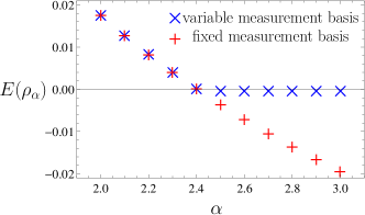
Figure 1: Entanglement detection of $\varrho_{\alpha}$ Eq. (63) with the help of Eq. (60). $E>0$ indicates entanglement. For $\times$ the measurement basis was optimized for each $\alpha$, whereas for $+$ we used the optimized basis for $\alpha=2$ for all $\alpha$. See the text for further details.

III Connections to existing criteria

As explained in the introduction, one of the main motivations of our paper is to present an unified view on several existing entanglement criteria. So in this section we show that several other entanglement criteria based on inequalities are applications of Eq. (4), although they were originally proven in a different way.

III.1 The criterion of Hillery and Zubairy

The entanglement criterion

$$|\langle A^{\dagger}B\rangle_{\mkern 1.0mu\mathrm{sep}\mkern 1.0mu}|^{2}\leq\langle A^{\dagger}AB^{\dagger}B\rangle_{\mkern 1.0mu\mathrm{sep}\mkern 1.0mu}$$ (66)

from Ref. Hillery et al. (2009) is a special case of Eq. (4) where we have set $A_{2}$ and $B_{1}$ equal to unity and $A_{1}=A^{\dagger}$ and $B_{2}=B$. By identifying $A=a^{m}$ with $a$ being the annihilation operator of system A and $B=(b^{\dagger})^{n}$ with $b^{\dagger}$ being the creation operator of system $B$ we rederive their original criterion

$$|\langle a^{m}(b^{\dagger})^{n}\rangle_{\mkern 1.0mu\mathrm{sep}\mkern 1.0mu}|^{2}\leq\langle(a^{\dagger})^{m}a^{m}(b^{\dagger})^{n}b^{b}\rangle_{\mkern 1.0mu\mathrm{sep}\mkern 1.0mu}$$ (67)

given in Ref. Hillery and Zubairy (2006). On the other hand,

$$|\langle a^{m}b^{n}\rangle_{\mkern 1.0mu\mathrm{sep}\mkern 1.0mu}|^{2}\leq\langle(a^{\dagger})^{m}a^{m}\rangle_{\mkern 1.0mu\mathrm{sep}\mkern 1.0mu}\langle(b^{\dagger})^{n}b^{b}\rangle_{\mkern 1.0mu\mathrm{sep}\mkern 1.0mu}$$ (68)

which was also derived in Ref. Hillery and Zubairy (2006) belongs to the special case

$$|\langle AB\rangle_{\mkern 1.0mu\mathrm{sep}\mkern 1.0mu}|^{2}\leq\langle A^{\dagger}A\rangle_{\mkern 1.0mu\mathrm{sep}\mkern 1.0mu}\langle B^{\dagger}B\rangle_{\mkern 1.0mu\mathrm{sep}\mkern 1.0mu}$$ (69)

where we have set $A_{1}$ and $B_{1}$ equal to unity.

Let us compare our entanglement criterion Eq. (4) with the criteria of the type Eq. (69) and Eq. (66) derived by Hillery and Zubairy for two qubit systems. By choosing

$$A_{1}=|1\rangle\langle 0|,\;A_{2}=|0\rangle\langle 0|,\;B_{1}=|1\rangle\langle 0|,\;B_{2}=|0\rangle\langle 0|$$ (70)

we obtain from Eq. (4) that all separable states $\varrho$ obey

$$|\varrho_{00,11}^{\mkern 1.0mu\mathrm{sep}\mkern 1.0mu}|^{2}\leq\varrho_{01,01}^{\mkern 1.0mu\mathrm{sep}\mkern 1.0mu}\varrho_{10,10}^{\mkern 1.0mu\mathrm{sep}\mkern 1.0mu}.$$ (71)

On the other hand Eq. (66) and Eq. (69) transform for the choice of and $A=A_{1}$ and $B=B_{1}$ into

$$|\varrho_{00,11}^{\mkern 1.0mu\mathrm{sep}\mkern 1.0mu}|^{2} \leq \varrho_{01,01}^{\mkern 1.0mu\mathrm{sep}\mkern 1.0mu}$$ (72)

$$|\varrho^{\mkern 1.0mu\mathrm{sep}\mkern 1.0mu}_{00,11}|^{2} \leq (\varrho^{\mkern 1.0mu\mathrm{sep}\mkern 1.0mu}_{10,10}+\varrho^{\mkern 1.0mu\mathrm{sep}\mkern 1.0mu}_{11,11})(\varrho^{\mkern 1.0mu\mathrm{sep}\mkern 1.0mu}_{01,01}+\varrho^{\mkern 1.0mu\mathrm{sep}\mkern 1.0mu}_{11,11}).$$ (73)

Due to the normalization of the state the coefficients of the matrix obey $0\leq\varrho_{jk,jk}\leq 1$ and therefore these criteria are weaker then Eq. (4). However, Eq. (66) requires only the estimation of a single expectation value or matrix entry instead of two for our criterion, and Eq. (69) only requires expectation values depending on single subsystems rather than correlations of both systems required for Eq. (4).

As suggested in Ref. Hillery and Zubairy (2006) Eq. (66) can be generalized to

$$|\langle\prod\limits_{k=1}^{N}A_{k}\rangle_{\mkern 1.0mu\mathrm{sep}\mkern 1.0mu}|^{2}\leq\langle\prod\limits_{k=1}^{j}A_{k}^{\dagger}A_{k}\prod\limits_{k=j+1}^{N}A_{k}A_{k}^{\dagger}\rangle_{\mkern 1.0mu\mathrm{sep}\mkern 1.0mu}$$ (74)

with $A_{k}$ being an operator acting on system $k$. This inequality holds true not only for seperable states, but also for biseperable states with respect to the partition ${1,2,\dots,j|j+1,\dots N}$. As a consequence, the inequality checks only if the state is biseperable with respect to a certain bipartition and does not check for real multipartite entanglement.

III.2 The criterion of Hillery et al.

In Ref. Hillery et al. (2010) the authors used a similar method to ours to generalize Eq. (69) to multipartite states: (i) First, they write the separable state as a convex set of pure product states. (ii) Then, they write every expectation value as the product of expectation values of single subsystems and apply the CS inequality to each of them. (iii) Finally, they use the Hölder inequality Eq. (56) to imply convexity. In this way they derive the criterion

$$|\langle\prod\limits_{k=1}^{n}A_{k}\rangle_{\mkern 1.0mu\mathrm{sep}\mkern 1.0mu}|\leq\prod\limits_{k=1}^{n}\langle(A^{\dagger}_{k}A_{k})^{n/2}\rangle_{\mkern 1.0mu\mathrm{sep}\mkern 1.0mu}^{1/n}$$ (75)

where $A_{k}$ denotes an operator acting on subsystem $k$. For their second criterion

$$|\langle\prod\limits_{k=1}^{n}A_{k}\rangle_{\mkern 1.0mu\mathrm{sep}\mkern 1.0mu}|\leq\langle\Big{(}\frac{1}{n}\sum\limits_{k=1}^{n}A^{\dagger}_{k}A_{k}\Big{)}^{n/2}\rangle_{\mkern 1.0mu\mathrm{sep}\mkern 1.0mu}$$ (76)

they used in addition that the geometric mean is smaller or equal than the arithmetic mean between step (ii) and (iii). For some states, both criteria are equal, for some Eq. (75) is stronger and for others Eq. (76) is stronger. However, both criteria used again only a single operator per subsystem. Furthermore, after step (ii) the property of product states was not used anymore whereas in our criteria we used these properties again to recombine expectation values. Therefore, our criterion is able to detect PPT states like $\varrho_{abc}$ defined in Eq. (61) whereas Eq. (75) cannot, which follows from the following theorem:

Theorem III.1

Assume a state $\varrho$ which is biseperable under some partitions in the following way: For any pair of subsystems $k$ and $j$ there there exists a bipartion $M|\bar{M}$ of the $N$ particles such that $k\in M$ and $j\in\bar{M}$ and the state $\varrho$ is biseparable for this bipartition $M|\bar{M}$. Then the criterion Eq. (75) cannot detect the entanglement of this state.

Note that by far not all bipartitions have to be separable to fulfill this condition, the minimal number of different bipartitions needed for this assumption scales like $\log_{2}(N)$.

Without loss of generality we assume there exists a bipartition $A_{1},\dots,A_{l}|A_{l+1},\dots A_{n}$, and therefore

$$|\langle\prod\limits_{k=1}^{n}A_{k}\rangle|\leq\sum\limits_{j}p_{j}\langle\prod\limits_{k=1}^{l}A_{k}^{\dagger}A_{k}\rangle_{j}^{1/2}\langle\prod\limits_{k=l+1}^{n}A_{k}^{\dagger}A_{k}\rangle_{j}^{1/2}.$$ (77)

With the help of the generalized Hölder inequality Eq. (56) we obtain

$$\begin{split}|\langle\prod\limits_{k=1}^{n}A_{k}\rangle|\leq&\Big{(}\sum\limits_{j}p_{j}\langle\prod\limits_{k=1}^{l}A_{k}^{\dagger}A_{k}\rangle_{j}^{n/2l}\Big{)}^{l/n}\\ &\times\Big{(}\sum\limits_{j}p_{j}\langle\prod\limits_{k=l+1}^{n}A_{k}^{\dagger}A_{k}\rangle_{j}^{n/2(n-l)}\Big{)}^{(n-l)/n}.\end{split}$$ (78)

by choosing $r=l/n$ and $s=(n-l)/n$. Again, with the help of Eq. (58) we find

$$\begin{split}|\langle\prod\limits_{k=1}^{n}A_{k}\rangle|\leq&\Big{(}\langle\prod\limits_{k=1}^{l}\left(A_{k}^{\dagger}A_{k}\right)^{n/2l}\rangle\Big{)}^{l/n}\\ &\times\Big{(}\langle\prod\limits_{k=l+1}^{n}\left(A_{k}^{\dagger}A_{k}\right)^{n/2(n-l)}\rangle\Big{)}^{(n-l)/n}.\end{split}$$ (79)

For each of the expectation values $\langle\prod A_{k}^{\dagger}A_{k}\rangle$ exist again a bipartition (with different $p_{j}$ and $\psi_{j}$) and therefore we arrive at

$$\begin{split}&\Big{(}\langle\prod\limits_{k=1}^{l}\left(A_{k}^{\dagger}A_{k}\Big{)}^{n/2l}\rangle\right)^{l/n}\\ =&\Big{(}\sum\limits_{j}p_{j}\langle\prod\limits_{k=1}^{x}\left(A_{k}^{\dagger}A_{k}\right)^{n/2l}\rangle_{j}\langle\prod\limits_{k=x+1}^{l}\left(A_{k}^{\dagger}A_{k}\right)^{n/2l}\rangle_{j}\Big{)}^{l/n}\\ \leq&\Big{(}\langle\prod\limits_{k=1}^{x}\left(A_{k}^{\dagger}A_{k}\right)^{n/2x}\rangle\Big{)}^{x/n}\\ &\times\Big{(}\langle\prod\limits_{k=x+1}^{l}\left(A_{k}^{\dagger}A_{k}\right)^{n/2(l-x)\rangle}\Big{)}^{(l-x)/n}\end{split}$$ (80)

by using again the generalized Hölder equation, now with $r=x/l$ and $s=(l-x)/l$ and Eq. (58). This argument can be applied until all expectation values are expectation values of a single subsystem and as a consequence we derive

$$|\langle\prod\limits_{k=1}^{n}A_{k}\rangle|\leq\prod\limits_{k=1}^{n}\langle(A^{\dagger}_{k}A_{k})^{n/2}\rangle^{1/n}.$$ (81)

This shows that the entanglement of an $N$-partite state $\varrho$ cannot be detected by Eq. (75), if for every two subsystem $i$ and $j$, there exist a bipartition of $\varrho$ where $i$ and $j$ can be separated. Furthermore, it shows that the criterion Eq. (75) is just a recursive application of the criterion Eq. (69) for bipartite entanglement from Hillery and Zubairy.

III.3 The criteria from Shchukin and Vogel

The criterion

$$\begin{split}|\langle a^{\dagger m}a^{n}a^{\dagger p}a^{q}b^{\dagger s}b^{r}b^{\dagger k}b^{l}\rangle_{\mkern 1.0mu\mathrm{sep}\mkern 1.0mu}|^{2}\leq&\langle a^{\dagger m}a^{n}a^{\dagger n}a^{m}b^{\dagger l}b^{k}b^{\dagger k}b^{l}\rangle_{\mkern 1.0mu\mathrm{sep}\mkern 1.0mu}\\ &\times\langle a^{\dagger q}a^{p}a^{\dagger p}a^{q}b^{\dagger s}b^{r}b^{\dagger r}b^{s}\rangle_{\mkern 1.0mu\mathrm{sep}\mkern 1.0mu}\end{split}$$ (82)

derived by Shchukin and Vogel in Shchukin and Vogel (2005) was originally proved with the help of the PPT criterion Peres (1996); Horodecki et al. (1996, 1997) and the matrix of moments.

Similarly, our criterion Eq. (4) follows also directly from the PPT criterion in the bipartite case. However, our criterion does not detect all NPT states. Nevertheless, Eq. (4) can be used to prove the criteria Eq. (82) by identifying

$$A_{1}=\left(a^{\dagger}\right)^{m}a^{n} A_{2}=\left(a^{\dagger}\right)^{p}a^{q},$$ , (83)

$$B_{1}=\left(b^{\dagger}\right)^{s}b^{r} B_{2}=\left(b^{\dagger}\right)^{k}b^{l}.$$ , (84)

As a consequence, all entangled states which can be detected with the criterion Eq. (82) derived by Shchukin and Vogel can be also detected with our criterion Eq. (4).

III.4 The criteria by Gühne and Seevinck

In Ref. Gühne and Seevinck (2010) the investigation of multiparticle entanglement was started by deriving criteria for bipartite entanglement,

$$|\varrho^{\mkern 1.0mu\mathrm{sep}\mkern 1.0mu}_{1,8}| \leq \sqrt{\varrho^{\mkern 1.0mu\mathrm{sep}\mkern 1.0mu}_{2,2}\varrho^{\mkern 1.0mu\mathrm{sep}\mkern 1.0mu}_{7,7}}$$ (85)

$$|\varrho^{\mkern 1.0mu\mathrm{sep}\mkern 1.0mu}_{1,8}| \leq \sqrt{\varrho^{\mkern 1.0mu\mathrm{sep}\mkern 1.0mu}_{3,3}\varrho^{\mkern 1.0mu\mathrm{sep}\mkern 1.0mu}_{6,6}}$$ (86)

$$|\varrho^{\mkern 1.0mu\mathrm{sep}\mkern 1.0mu}_{1,8}| \leq \sqrt{\varrho^{\mkern 1.0mu\mathrm{sep}\mkern 1.0mu}_{4,4}\varrho^{\mkern 1.0mu\mathrm{sep}\mkern 1.0mu}_{5,5}}$$ (87)

with the standard product basis $\{|000\rangle,|001\rangle,\dots,|111\rangle\}$. Although they were proven in another way, they directly follow from our criterion Eq. (4) by interpreting the systems $A$ and $B$ as two sets of systems instead of two single systems.

Using the fact that the geometric mean is smaller or equal to the arithmetic mean, which denotes

$$\prod\limits_{j=1}^{N}a_{k}^{1/N}\leq\frac{1}{N}\sum\limits_{j=1}^{N}a_{k}$$ (88)

these three equations lead to the criteria

$$|\varrho^{\mkern 1.0mu\mathrm{sep}\mkern 1.0mu}_{1,8}| \leq \frac{1}{2}(\varrho^{\mkern 1.0mu\mathrm{sep}\mkern 1.0mu}_{2,2}+\varrho^{\mkern 1.0mu\mathrm{sep}\mkern 1.0mu}_{7,7})$$ (89)

$$|\varrho^{\mkern 1.0mu\mathrm{sep}\mkern 1.0mu}_{1,8}| \leq \frac{1}{2}(\varrho^{\mkern 1.0mu\mathrm{sep}\mkern 1.0mu}_{3,3}+\varrho^{\mkern 1.0mu\mathrm{sep}\mkern 1.0mu}_{6,6})$$ (90)

$$|\varrho^{\mkern 1.0mu\mathrm{sep}\mkern 1.0mu}_{1,8}| \leq \frac{1}{2}(\varrho^{\mkern 1.0mu\mathrm{sep}\mkern 1.0mu}_{4,4}+\varrho^{\mkern 1.0mu\mathrm{sep}\mkern 1.0mu}_{5,5})$$ (91)

used also in Ref. Dür and Cirac (2000).

By a convex combination of the three equations Eq. (85), Eq. (86) and Eq. (87) one can derive the condition

$$|\varrho^{\mkern 1.0mu\mathrm{sep}\mkern 1.0mu}_{1,8}|\leq\sqrt{\varrho^{\mkern 1.0mu\mathrm{sep}\mkern 1.0mu}_{2,2}\varrho^{\mkern 1.0mu\mathrm{sep}\mkern 1.0mu}_{7,7}}+\sqrt{\varrho^{\mkern 1.0mu\mathrm{sep}\mkern 1.0mu}_{3,3}\varrho^{\mkern 1.0mu\mathrm{sep}\mkern 1.0mu}_{6,6}}+\sqrt{\varrho^{\mkern 1.0mu\mathrm{sep}\mkern 1.0mu}_{4,4}\varrho^{\mkern 1.0mu\mathrm{sep}\mkern 1.0mu}_{5,5}}$$ (92)

which is valid for all biseparable three qubit states, and is only violated by fully entangled states. This, of course, can not be derived by our framework, since we are only dealing with criteria excluding full separability.

However, by multiplying the three equations Eq. (85), Eq. (86) and Eq. (87) one finds the inequality

$$|\varrho^{\mkern 1.0mu\mathrm{sep}\mkern 1.0mu}_{1,8}|\leq(\varrho^{\mkern 1.0mu\mathrm{sep}\mkern 1.0mu}_{2,2}\varrho^{\mkern 1.0mu\mathrm{sep}\mkern 1.0mu}_{3,3}\varrho^{\mkern 1.0mu\mathrm{sep}\mkern 1.0mu}_{4,4}\varrho^{\mkern 1.0mu\mathrm{sep}\mkern 1.0mu}_{5,5}\varrho^{\mkern 1.0mu\mathrm{sep}\mkern 1.0mu}_{6,6}\varrho^{\mkern 1.0mu\mathrm{sep}\mkern 1.0mu}_{7,7})^{1/6}.$$ (93)

which is valid for all fully seperable states. This inequality can be proven also directly by using our scheme from Sec. II.2.1 to develop the criterion

$$\begin{split}&|\langle A_{1}A_{2}B_{1}B_{2}C_{1}C_{2}\rangle_{\mkern 1.0mu\mathrm{sep}\mkern 1.0mu}|\\ \leq&\sqrt[6]{\langle A_{2}^{\dagger}A_{2}B_{2}^{\dagger}B_{2}C_{1}C_{1}^{\dagger}\rangle_{\mkern 1.0mu\mathrm{sep}\mkern 1.0mu}\langle A_{2}^{\dagger}A_{2}B_{1}B_{1}^{\dagger}C_{2}^{\dagger}C_{2}\rangle_{\mkern 1.0mu\mathrm{sep}\mkern 1.0mu}}\\ &\times\sqrt[6]{\langle A_{1}A_{1}^{\dagger}B_{2}^{\dagger}B_{2}C_{1}C_{1}^{\dagger}\rangle_{\mkern 1.0mu\mathrm{sep}\mkern 1.0mu}\langle A_{1}A_{1}^{\dagger}B_{2}^{\dagger}B_{2}C_{2}^{\dagger}C_{2}\rangle_{\mkern 1.0mu\mathrm{sep}\mkern 1.0mu}}\\ &\times\sqrt[6]{\langle A_{2}^{\dagger}A_{2}B_{1}B_{1}^{\dagger}C_{1}C_{1}^{\dagger}\rangle_{\mkern 1.0mu\mathrm{sep}\mkern 1.0mu}\langle A_{1}A_{1}^{\dagger}B_{1}B_{1}^{\dagger}C_{2}^{\dagger}C_{2}\rangle_{\mkern 1.0mu\mathrm{sep}\mkern 1.0mu}},\end{split}$$ (94)

and by using the operators defined in Eq. (II.2.2) and Eq. (62). Since Eq. (93) is a product of three criteria for bi-separability, it cannot detect the entanglement of PPT states like $\varrho_{abc}$ Eq. (61). However, as noted in Ref. Gühne and Seevinck (2010) in Eq. (93) it is possible to substitute certain matrix entries $\varrho_{j,j}$ by others, for example $\varrho_{2,2}\varrho_{3,3}\rightarrow\varrho_{1,1}\varrho_{4,4}$ to get different criteria. The substitution of matrix entries is equivalent to a different combination of the operators $A_{j}$, $B_{j}$ and $C_{j}$ in our scheme. These new criteria are able to detect PPT states, for example the criterion

$$|\varrho_{1,8}^{\mkern 1.0mu\mathrm{sep}\mkern 1.0mu}|\leq(\varrho^{\mkern 1.0mu\mathrm{sep}\mkern 1.0mu}_{1,1}(\varrho^{\mkern 1.0mu\mathrm{sep}\mkern 1.0mu}_{4,4})^{2}\varrho^{\mkern 1.0mu\mathrm{sep}\mkern 1.0mu}_{5,5}\varrho^{\mkern 1.0mu\mathrm{sep}\mkern 1.0mu}_{6,6}\varrho^{\mkern 1.0mu\mathrm{sep}\mkern 1.0mu}_{7,7})^{1/6}$$ (95)

derived by substituting $\varrho_{2,2}\varrho_{3,3}\rightarrow\varrho_{1,1}\varrho_{4,4}$ in Eq. (93), leads to $1\leq(abc)^{-1/6}$ for the PPT-state $\varrho_{abc}$ given in Eq. (61) which is violated for $abc>1$. With a second similar equations, the entanglement can be detected for $1\leq(abc)^{1/6}$. As a consequence, the criteria of Ref. Gühne and Seevinck (2010) detect entanglement if $abc\neq 1$ similar to our criterion shown in Sec. II.2.2. However, by translating our criterion from Sec. II.2.2 into density matrix representation

$$|\varrho^{\mkern 1.0mu\mathrm{sep}\mkern 1.0mu}_{1,8}|\leq\sqrt[4]{\varrho^{\mkern 1.0mu\mathrm{sep}\mkern 1.0mu}_{1,1}\varrho^{\mkern 1.0mu\mathrm{sep}\mkern 1.0mu}_{4,4}\varrho^{\mkern 1.0mu\mathrm{sep}\mkern 1.0mu}_{6,6}\varrho^{\mkern 1.0mu\mathrm{sep}\mkern 1.0mu}_{7,7}}$$ (96)

we see that the criterion of Ref. Gühne and Seevinck (2010) is a weighted mean of the criteria Eq. (87) and Eq. (96). Therefore Eq. (95) is only equally or less strong than testing Eq. (87) and Eq. (96) separately. This was also noted in Ref. Gühne (2011).

III.5 The criterion by Huber et al.

In Ref. Huber et al. (2010) the criterion

$$\begin{split}&\sqrt{\text{Re\,}\left[\langle\Phi_{\mkern 1.0mu\mathrm{ps}\mkern 1.0mu}|(\mathbbm{1}_{A}\otimes\Pi_{B})^{\dagger}\varrho_{\mkern 1.0mu\mathrm{sep}\mkern 1.0mu}^{\otimes m}(\Pi_{A}\otimes\mathbbm{1}_{B})|\Phi_{\mkern 1.0mu\mathrm{ps}\mkern 1.0mu}\rangle\right]}\\ &\leq\sqrt{\langle\Phi_{\mkern 1.0mu\mathrm{ps}\mkern 1.0mu}|\varrho_{\mkern 1.0mu\mathrm{sep}\mkern 1.0mu}^{\otimes m}|\Phi_{\mkern 1.0mu\mathrm{ps}\mkern 1.0mu}\rangle}\end{split}$$ (97)

where $\varrho_{\mkern 1.0mu\mathrm{sep}\mkern 1.0mu}^{\otimes m}$ is an m-fold tensor product of the density matrix $\varrho_{\mkern 1.0mu\mathrm{sep}\mkern 1.0mu}$, $|\Phi_{\mkern 1.0mu\mathrm{ps}\mkern 1.0mu}\rangle$ being a product state of the m-tupled system and $\Pi$ being the cyclic permutation operator. For the case $m=2$ this criterion transforms exactly into Eq. (21) and is therefore equivalent to our criterion if one chooses the operators to be projectors on a single state.

For the case $m>2$ the criteria can be led back to a combination of the criterion with $m=2$ and different states $|\Phi_{\mkern 1.0mu\mathrm{ps}\mkern 1.0mu}\rangle$. Therefore, the criteria for $m>2$ do not show any advances compared to the criterion for $m=2$.

In the multipartite case, the generalization of the criterion for $m=2$ reads

$$\begin{split}\sqrt{\langle\Phi_{\mkern 1.0mu\mathrm{ps}\mkern 1.0mu}|\varrho_{\mkern 1.0mu\mathrm{bs}\mkern 1.0mu}^{\otimes m}\bf{\Pi}|\Phi_{\mkern 1.0mu\mathrm{ps}\mkern 1.0mu}\rangle}&\\ -\sum\limits_{j}\sqrt{\langle\Phi_{\mkern 1.0mu\mathrm{ps}\mkern 1.0mu}|\mathcal{P}^{\dagger}_{j}\varrho_{\mkern 1.0mu\mathrm{bs}\mkern 1.0mu}^{\otimes m}\mathcal{P}_{j}|\Phi_{\mkern 1.0mu\mathrm{ps}\mkern 1.0mu}\rangle}&\leq 0\end{split}$$ (98)

which is valid for all biseparable (bs) states. Here, the operator $\bf{\Pi}$ performs simultaneous permutations on all subsystems and $\mathcal{P}_{j}$ performs only a permutation on the subsystem $A_{j}$ for the different bipartitions $j$.

In a similar way, our criteria can be transformed to detect only genuine multipartite entanglement. Let $X_{k}$ and $Y_{k}$ be operators acting on subsystem $k$. Furthermore, let $S_{j}$ be the set of all pure biseparable states which are biseparable under the bipartition $A_{j}|B_{j}$. As a consequence, every biseparable state

$$\varrho_{\mkern 1.0mu\mathrm{bs}\mkern 1.0mu}\equiv\sum\limits_{j}\sum\limits_{s_{j}\in S_{j}}p_{s_{j}}|s_{j}\rangle\langle s_{j}|$$ (99)

can be written as a convex combination of states $s_{j}$ belonging to different sets $S_{j}$ with weights $p_{s_{j}}$. In this case we find the inequality

$$\begin{split}\big{|}\langle\prod\limits_{k}X_{k}Y_{k}\rangle_{\mkern 1.0mu\mathrm{bs}\mkern 1.0mu}\big{|}\leq&\sum\limits_{j}\sum\limits_{s_{j}\in S_{j}}p_{s_{j}}\sqrt{\langle\prod\limits_{k\in A_{j}}X_{k}X_{k}^{\dagger}\prod\limits_{k\in Bj}Y_{k}^{\dagger}Y_{k}\rangle_{s_{j}}}\\ &\times\sqrt{\langle\prod\limits_{k\in A_{j}}Y_{k}^{\dagger}Y_{k}\prod\limits_{k\in Bj}X_{k}X_{k}^{\dagger}\rangle_{s_{j}}}.\end{split}$$ (100)

Since $X_{k}X_{k}^{\dagger}$ and $Y_{k}^{\dagger}Y_{k}$ are positive operators we increase the right side of this inequality be increasing the summation range from $S_{j}$ to $S=\cup S_{j}$. As a consequence, we obtain the criterion

$$\begin{split}\big{|}\langle\prod\limits_{k}X_{k}Y_{k}\rangle_{\mkern 1.0mu\mathrm{bs}\mkern 1.0mu}\big{|}\leq&\sum\limits_{j}\sqrt{\langle\prod\limits_{k\in A_{j}}X_{k}X_{k}^{\dagger}\prod\limits_{k\in Bj}Y_{k}^{\dagger}Y_{k}\rangle_{{\mkern 1.0mu\mathrm{bs}\mkern 1.0mu}}}\\ &\times\sqrt{\langle\prod\limits_{k\in A_{j}}Y_{k}^{\dagger}Y_{k}\prod\limits_{k\in Bj}X_{k}X_{k}^{\dagger}\rangle_{{\mkern 1.0mu\mathrm{bs}\mkern 1.0mu}}}.\end{split}$$ (101)

for genuine multipartite entanglement.

IV Conclusion

In this paper we have shown how to develop entanglement criteria with the help of the Cauchy-Schwarz and the Hölder inequality and the properties of separable states. In the bipartite case, our criterion is strongly connected to the PPT-criterion and only NPT-states can be detected. We demonstrate that all two-qubit states and all NPT-entangled states mixed with white noise can be detected with our criteria. However, not all NPT-states can be detected with our criterion, since it operates in a $2\times 2$ dimensional subspace only. However, we suggested some ideas for an additional entanglement criterion which may detect such states.

We generalized our criteria to the multipartite case with the help of the Hölder inequality. We demonstrated that with our scheme it is possible to detect the entanglement of states which are separable under every bipartite split. As a consequence, our criteria are not restricted to NPT entangled states in the multipartite case. We also explained how to transform our criteria in such a way that they detect only genuine multipartite entanglement.

Furthermore, we showed that some already existing criteria for bipartite and multipartite entanglement which have been proven already with other methods, are direct consequences of the Cauchy-Schwarz inequality. As a consequence, our method to derive entanglement criteria is more fundamental. We demonstrated that criteria which use two operators per subsystems are in general stronger than criteria which use only a single operator per subsystem. As a consequence, our methods lead to stronger entanglement criteria.

V Acknowledgement

S.W. thanks Suhail Zubairy for fruitful discussions. This work has been supported by the EU (Marie Curie CIG 293993/ENFOQI and Marie Curie IEF 302021/QUACOCOS), the BMBF (Chist-Era Project QUASAR), the FQXi Fund (Silicon Valley Community Foundation), and the DFG.

References

- Peres (1996) A. Peres, Phys. Rev. Lett. 77, 1413 (1996).
- Horodecki et al. (1996) P. Horodecki, R. Horodecki, and M. Horodecki, Phys. Lett. A 223, 1 (1996).
- Shchukin and Vogel (2005) E. Shchukin and W. Vogel, Phys. Rev. Lett. 95, 230502 (2005).
- Hillery and Zubairy (2006) M. Hillery and M. S. Zubairy, Phys. Rev. Lett. 96, 050503 (2006).
- Gühne and Seevinck (2010) O. Gühne and M. Seevinck, New J. of Phys. 12, 053002 (2010).
- Hillery et al. (2010) M. Hillery, H. T. Dung, and H. Zheng, Phys. Rev. A 81, 062322 (2010).
- Dür and Cirac (2000) W. Dür and J. I. Cirac, Phys. Rev. A. 61, 042314 (2000).
- Huber et al. (2010) M. Huber, F. Mintert, A. Gabriel, and B. C. Hiesmayr, Phys. Rev. Lett. 104, 210501 (2010).
- Cauchy (1821) A.-L. Cauchy, Analyse algébrique (Imprimerie Royale, Paris, 1821).
- Hillery et al. (2009) M. Hillery, H. T. Dung, and J. Niset, Phys. Rev. A 80, 052335 (2009).
- Johnston (2013) N. Johnston, Phys. Rev. A 87, 064302 (2013).
- Rana (2013) S. Rana, Phys. Rev. A 87, 054301 (2013).
- Sanpera et al. (1998) A. Sanpera, R. Tarrach, and G. Vidal, Phys. Rev. A 58, 826 (1998).
- Augusiak et al. (2008) R. Augusiak, M. Demianowicz, and P. Horodecki, Phys. Rev. A 77, 030301 (2008).
- Horodecki et al. (1998) M. Horodecki, P. Horodecki, and R. Horodecki, Phys. Rev. Lett. 80, 5239 (1998).
- Werner (1989) R. F. Werner, Phys. Rev. A 40, 4277 (1989).
- Hardy et al. (1934) G. Hardy, J. E. Littlewood, and G. Pólya, Inequalities (Cambridge Univ. Press, London, 1934).
- Acín et al. (2001) A. Acín, D. Bruß, M. Lewenstein, and A. Sanpera, Phys. Rev. Lett. 87, 040401 (2001).
- Kay (2011) A. Kay, Phys. Rev. A 83, 020303 (2011).
- Gühne (2011) O. Gühne, Phys. Lett. A 375, 406 (2011).
- Horodecki et al. (1997) P. Horodecki, R. Horodecki, and M. Horodecki, Phys. Lett. A 232, 333 (1997).