Depletion effects in colloid-polymer solutions

Abstract

The surface tension, the adsorption, and the depletion thickness of polymers close to a single nonadsorbing colloidal sphere are computed by means of Monte Carlo simulations. We consider polymers under good-solvent conditions and in the thermal crossover region between good-solvent and $\theta$ behavior. In the dilute regime we consider a wide range of values of $q$, from $q=0$ (planar surface) up to $q\approx 30$-50, while in the semidilute regime, for $\rho_{p}/\rho_{p}^{*}\leq 4$ ($\rho_{p}$ is the polymer concentration and $\rho_{p}^{*}$ is its value at overlap), we only consider $q=0,0.5,1$ and 2. The results are compared with the available theoretical predictions, verifying the existing scaling arguments. Field-theoretical results, both in the dilute and in the semidilute regime, are in good agreement with the numerical estimates for polymers under good-solvent conditions.

I Introduction

The study of the fluid phases in mixtures of colloids and nonadsorbing neutral polymers has become increasingly important in recent years; see Refs. Poon-02 ; FS-02 ; TRK-03 ; MvDE-07 ; FT-08 ; ME-09 for recent reviews. These systems show a very interesting phenomenology, which only depends to a large extent on the nature of the polymer-solvent system and on the ratio $q\equiv\hat{R}_{g}/R_{c}$, where $\hat{R}_{g}$ is the zero-density radius of gyration of the polymer and $R_{c}$ is the radius of the colloid. Experiments and numerical simulations indicate that polymer-colloid mixtures have a fluid-solid coexistence line and, for $q>q^{*}$, where Poon-02 $q^{*}\approx 0.3$-0.4, also a fluid-fluid coexistence line between a colloid-rich, polymer-poor phase (colloid liquid) and a colloid-poor, polymer-rich phase (colloid gas). On the theoretical side, research has mostly concentrated on mixtures of neutral spherical colloids and polymers in solutions under good-solvent or $\theta$ conditions. In the former case, predictions for the colloid-polymer interactions have been obtained by using full-monomer representations of polymers (for instance, the self-avoiding walk model was used in Refs. LBMH-02-a ; LBMH-02-b ), field-theoretical methods EHD-96 ; HED-99 ; MEB-01 , or fluid integral equations FS-01 . Moreover, some general properties have been derived by using general scaling arguments deGennes-CR79 ; JLdG-79 ; Odijk-96 . At the $\theta$ point, the analysis is simpler, since polymers behave approximately as ideal chains. These theoretical results have then been used as starting points to develop a variety of coarse-grained models and approximate methods, see Refs. LBHM-00 ; LBMH-02-a ; FT-08 and references therein, which have been employed to predict colloid-polymer phase diagrams.

In this paper, we consider polymer solutions that either show good-solvent behavior or are in the thermal crossover region between good-solvent and $\theta$ conditions. We study the solvation of a single colloid in the solution, assuming that the monomer-colloid potential is purely repulsive. We determine the distribution of the polymer chains around a single colloidal particle, which is the simplest property that characterizes polymer-colloid interactions. We investigate numerically, by means of Monte Carlo simulations, how it depends on the quality of the solution, which is parametrized Nickel-91 ; DPP-thermal in terms of the second-virial combination $A_{2,pp}=B_{2,pp}/\hat{R}_{g}^{3}$, where $B_{2,pp}$ is the second virial coefficient and $\hat{R}_{g}$ is the zero-density radius of gyration. This adimensional combination varies between 5.50 in the good-solvent case CMP-06 and zero ($\theta$ point). Beside good-solvent solutions, we consider two intermediate cases: solutions such that $A_{2,pp}$ is approximately one half of the good-solvent value, which show intermediate properties betweeen good-solvent and $\theta$ behavior, and solutions such that $A_{2,pp}$ is 20% of the good-solvent value, which are close to the $\theta$ point. In each case we compute the polymer density profile around the colloid. These results are used to determine thermodynamic properties, like the surface tension and the adsorption Widom , which are then compared with the available theoretical predictions. Note that an analysis of the polymer depletion around a colloid in the thermal crossover region was already performed in Refs. ALH-04 ; PH-06 , but without a proper identification of the universal crossover limit Sokal-94 . Here, we wish to perform a much more careful analysis of the crossover behavior, following Refs. CMP-08 ; DPP-thermal . We focus on the dilute and semidilute regimes, in which the monomer density is small and a universal behavior, i.e., independent of chemical details, is obtained in the limit of large degree of polymerization. In the dilute regime, in which polymer-polymer overlaps are rare, solvation properties are determined for a wide range of values of $q$, from 0 up to 30-50. In the semidilute regime, simulations of systems with large $q$ require considering a large number of colloids, which makes Monte Carlo simulations very expensive. Hence, we only present results for $q=0,0.5,1$ and 2.

The paper is organized as follows. In Sec. II we define the basic quantities we wish to determine. First, in Sec. II.1 and II.2 we introduce the surface tension, the adsorption, and the depletion thickness, and discuss their relation to the density profile of the polymers around the colloid. In Sec. II.3 we discuss the low-density behavior and the relation between solvation properties and colloid-polymer virial coefficients that parametrize the (osmotic) pressure of a polymer-colloid binary solution in the low-density limit. Sec. II.4 discusses the different behavior that are expected as a function of $q$ and density and gives an overview of theoretical and numerical predictions. Sec. III summarizes our polymer model and gives a brief discussion on how one can parametrize in a universal fashion the crossover between the good-solvent and the $\theta$ behavior (for more details, see Ref. DPP-thermal ). In Sec. IV we present our results for the dilute regime, while finite-density results are presented in Sec. V. Sec. VI discusses a simple coarse-grained model in which each polymer is represented by a monoatomic molecule, which represents a more rigorous version of the well-known Asakura-Oosawa-Vrij model. In Sec. VII we present our conclusions. Two appendices are included, one explaining how to compute the virial coefficients of a binary mixture of flexible molecules, and one discussing the small-$q$ behavior of the virial coefficients. Tables of results are reported in the supplementary material.

II Adsorption and depletion thickness

II.1 Definitions

Let us consider a solution of nonadsorbing polymers in the grand canonical ensemble at fixed volume $V$ and chemical potential $\mu_{p}$. Temperature is also present, but, since it does not play any role in our discussion, we will omit writing it explicitly in the following. Let us indicate with $\Omega(\mu_{p},V)$ the corresponding grand potential. Let us now add a spherical colloidal particle of radius $R_{c}$ to the solution and let $\Omega_{c}(\mu_{p},V)$ be the corresponding grand potential. The insertion free energy can be written as the sum of two terms, one proportional to the volume $V_{c}={4\over 3}\pi R_{c}^{3}$ of the colloid and one proportional to its surface area $A_{c}=4\pi R_{c}^{2}$ Widom :

$$\Omega_{c}(\mu_{p},V)-\Omega(\mu_{p},V)=PV_{c}+\gamma A_{c},$$ (1)

where $P$ is the bulk pressure and $\gamma$ is the surface tension. The latter quantity can be related to the adsorption $\Gamma(\mu_{p})$ defined in terms of the change in the mean number of polymers due to the presence of the colloid:

$$\langle N_{p}\rangle^{(c)}-\langle N_{p}\rangle=-\rho_{p}V_{c}+\Gamma A_{c},$$ (2)

where $N_{p}$ indicates the numbers of polymers present in the solution, $\langle\cdot\rangle^{(c)}$ and $\langle\cdot\rangle$ are averages in the presence and in the absence of the colloidal particle, respectively. Differentiating Eq. (1) with respect to $\mu_{p}$, we obtain

$$\Gamma(\mu_{p})=-\left(\frac{\partial\gamma}{\partial\mu_{p}}\right)_{T,V}.$$ (3)

We also define the average bulk polymer density $\rho_{p}$ as

$$\rho_{p}(\mu_{p})=-{1\over V}\left({\partial\Omega\over\partial\mu_{p}}\right)_{T,V}.$$ (4)

The surface tension can also be defined in the canonical ensemble, as a function of the bulk polymer density $\rho_{p}$. Then, we have

$$\Gamma(\rho_{p})=-\left(\frac{\partial\beta\gamma}{\partial\rho_{p}}\right)_{T,V}{\rho_{p}\over K_{p}(\rho_{p})},$$ (5)

where

$$K_{p}=\left({\partial\beta P\over\partial\rho_{p}}\right)_{T,V},$$ (6)

for the bulk system ($\beta=1/k_{B}T$ as usual).

The adsorption coefficient can be easily related to the polymer density profile around the colloid. Assume that each polymer consists of $L$ monomers and define the average bulk monomer density $\rho_{{\rm mon}}=L\rho_{p}$. Then, we write

$$\langle N_{p}\rangle^{(c)}-\langle N_{p}\rangle$$

$$=\,\int d^{3}{\bf r}\,\left[{1\over L}\left\langle\sum_{\alpha i}\delta({\bf R}_{c}-{\bf r}_{\alpha}^{(i)}-{\bf r})\right\rangle^{(c)}-\rho_{p}(\mu_{p})\right],$$ (7)

where the average is performed at chemical potential $\mu_{p}$ and volume $V$, ${\bf R}_{c}$ is the colloid position, and ${\bf r}_{\alpha}^{(i)}$, $\alpha=1,\ldots,L$, $i=1,\ldots N_{p}$, are the monomer positions. If we now define the monomer-colloid pair correlation function

$$g_{{\rm mon},cp}(r;\mu_{p})={1\over\rho_{{\rm mon}}}\left\langle\sum_{\alpha i}\delta({\bf R}_{c}-{\bf r}_{\alpha}^{(i)}-{\bf r})\right\rangle^{(c)},$$ (8)

and the integral

$$G_{{\rm mon},cp}(\mu_{p})=\int d{\bf r}\,[g_{{\rm mon},cp}(r;\mu_{p})-1],$$ (9)

we obtain

$$\Gamma(\mu_{p})={\rho_{p}(\mu_{p})\over A_{c}}\left[G_{{\rm mon},cp}(\mu_{p})+V_{c}\right].$$ (10)

Since $g_{{\rm mon},cp}(r;\mu_{p})=0$ for $r\leq R_{c}$, a more transparent relation is obtained by defining

$$\hat{G}_{{\rm mon},cp}(\mu_{p})=4\pi\int_{R_{c}}^{\infty}r^{2}d{r}\,[g_{{\rm mon},cp}(r;\mu_{p})-1],$$ (11)

in which one only integrates the density profile outside the colloid. Since ${G}_{{\rm mon},cp}(\mu_{p})=\hat{G}_{{\rm mon},cp}(\mu_{p})-V_{c}$, we have

$$\Gamma(\mu_{p})={\rho_{p}(\mu_{p})\over A_{c}}\hat{G}_{{\rm mon},cp}(\mu_{p}).$$ (12)

In the previous discussion we have considered the monomer-colloid correlation function, but it is obvious that any other polymer-colloid distribution function could be used. In order to compare our results with those obtained in coarse-grained models (we will discuss them in Sec. VI), we will also use the pair distribution function between the colloid and the polymer centers of mass. If ${\bf r}_{\alpha}^{(i)}$, $\alpha=1,\ldots,L$, are the positions of the monomers belonging to polymer $i$, we first define the polymer center of mass

$${\bf r}^{(i)}_{CM}={1\over L}\sum_{\alpha}{\bf r}_{\alpha}^{(i)}.$$ (13)

Then, the pair distribution function between a colloid and a polymer center of mass is defined by

$$g_{CM,cp}(r;\mu_{p})={1\over\rho_{p}}\left\langle\sum_{i}\delta({\bf R}_{c}-{\bf r}_{CM}^{(i)}-{\bf r})\right\rangle^{(c)},$$ (14)

where the average is taken at a given value $\mu_{p}$. In terms of this quantity

$$\Gamma(\mu_{p}) = {\rho_{p}(\mu_{p})\over A_{c}}[V_{c}+G_{CM,cp}(\mu_{p})],$$ (15)

$$G_{CM,cp}(\mu_{p}) = 4\pi\int_{0}^{\infty}r^{2}dr\,[g_{{CM},cp}(r;\mu_{p})-1].$$

If we define $\hat{G}_{CM,cp}(\mu_{p})=V_{c}+G_{CM,cp}(\mu_{p})$, we can write a relation analogous to Eq. (12). Comparison of Eqs. (12) and (15) implies $G_{CM,cp}=G_{{\rm mon},cp}$ and $\hat{G}_{CM,cp}=\hat{G}_{{\rm mon},cp}$, hence in the following we will simply refer to these quantities as $G_{cp}$ and $\hat{G}_{cp}$.

It is interesting to relate the pair correlation functions $g_{cp}(r;\mu_{p})$ to the analogous correlation functions $\hat{g}_{cp}(r;\mu_{p},\mu_{c})$ that are appropriate for a binary system consisting of polymers and colloids at polymer and colloid chemical potentials $\mu_{p}$ and $\mu_{c}$, respectively. Indeed, one can show that, in the limit $\mu_{c}\to-\infty$, i.e., when the colloid density goes to zero, one has

$$g_{cp}(r;\mu_{p})=\lim_{\mu_{c}\to-\infty}\hat{g}_{cp}(r;\mu_{p},\mu_{c}).$$ (16)

Eq. (16) allows us to relate $G_{cp}$ to thermodynamic properties of the binary mixture in the limit of vanishing colloid density. For this purpose we use the Kirkwood-Buff relations between structural and thermodynamic properties of fluid mixtures KB-51 ; BenNaim . The integral $G_{cp}$, which is relevant to determine adsorption properties, corresponds to one of the Kirkwood-Buff integrals KB-51 ; BenNaim defined as

$$G_{\alpha\beta}=\int d{\bf r}\,(g_{\alpha\beta}(r)-1),$$ (17)

where $\alpha$ and $\beta$ label the different species of the mixture. The integrals $G_{\alpha\beta}$ can be related to derivatives of the pressure with respect to the polymer and colloid densities. For $\rho_{c}=0$ we have KB-51 ; BenNaim

$$K_{c} = \left({\partial\beta P\over\partial\rho_{c}}\right)_{\rho_{p}}=1-{\rho_{p}G_{cp}\over 1+\rho_{p}G_{pp}},$$ (18)

$$K_{p} = \left({\partial\beta P\over\partial\rho_{p}}\right)_{\rho_{c}=0}={1\over 1+\rho_{p}G_{pp}},$$ (19)

which imply

$$G_{cp}={1-K_{c}\over\rho_{p}K_{p}}.$$ (20)

Eqs. (12) and (5) can then be rewritten as

$$\Gamma = {1\over A_{c}}\left[{1-K_{c}\over K_{p}}+\rho_{p}V_{c}\right],$$ (21)

$$\beta\gamma = {1\over A_{c}}\int_{0}^{\rho_{p}}{K_{c}-1\over\rho_{p}^{\prime}}d\rho_{p}^{\prime}-\beta P{V_{c}\over A_{c}}.$$ (22)

II.2 Depletion thickness

Depletion effects can be equivalently parametrized by introducing the depletion thickness $\delta_{s}$ FT-07 ; FST-07 ; FT-08 ; LT-11 , which is an average width of the depleted layer around the colloid. It is defined in terms of the integral $G_{cp}$ as

$$\frac{4\pi}{3}\left(R_{c}+\delta_{s}\right)^{3}=-G_{cp}=V_{c}-\hat{G}_{cp},$$ (23)

so that

$${\delta_{s}\over R_{c}}=\left(1-{\hat{G}_{cp}\over V_{c}}\right)^{1/3}-1.$$ (24)

Since $\delta_{s}$ is only determined by $G_{cp}$, knowledge of $\delta_{s}$ is completely equivalent to that of the adsorption. The two quantites are related by

$$\Gamma=-{\rho_{p}V_{c}\over A_{c}}\left[\left(1+\delta_{s}/R_{c}\right)^{3}-1\right].$$ (25)

As we shall discuss below, $\delta_{s}/R_{c}\to 0$ for large polymer densities, hence in this limit

$$\Gamma=-\rho_{p}\delta_{s}.$$ (26)

It is interesting to discuss the limit $q\to 0$, in which the colloid degenerates into an impenetrable plane. Setting $r=R_{c}+z$ in Eq. (11), we obtain

$$\hat{G}_{cp}=4\pi\int_{0}^{\infty}dz\,(R_{c}+z)^{2}[g_{{\rm mon},cp}(R_{c}+z)-1].$$ (27)

For $R_{c}\to\infty$, we have $g_{{\rm mon},cp}(R_{c}+z)\approx g_{\rm mon,pl}(z)$, where $g_{\rm mon,pl}(z)$ is the pair distribution function between an impenetrable plane at $z=0$ and a polymer. Then, we obtain for $R_{c}\to\infty$

$$\hat{G}_{cp}=4\pi R_{c}^{2}G_{pl},$$ (28)

with

$$G_{pl}=\int_{0}^{\infty}dz\,[g_{\rm mon,pl}(z)-1].$$ (29)

Taking the limit $R_{c}\to\infty$ in Eqs. (24) and (25), we obtain

$$\delta_{s}=-{\Gamma\over\rho_{p}}=-G_{pl}.$$ (30)

II.3 Low-density expansions

For $\rho_{p}\to 0$ the depletion thickness $\delta_{s}$ and the surface quantities $\Gamma$ and $\gamma$ can be related to the virial coefficients that parametrize the expansion of the pressure of a binary colloid-polymer system in powers of the concentrations. These relations have already been discussed in the literature Bellemans-63 ; SS-80 ; MQR-87 ; YSEK-13 . They can be easily derived by using Eqs. (21) and (22). We start by expanding the pressure as

$$\beta P=\rho_{c}+\rho_{p}+B_{2,cc}\rho_{c}^{2}+B_{2,pp}\rho_{p}^{2}+B_{2,cp}\rho_{c}\rho_{p}$$

$$\quad+B_{3,ccc}\rho_{c}^{3}+B_{3,ppp}\rho_{p}^{3}+B_{3,ccp}\rho_{c}^{2}\rho_{p}+B_{3,cpp}\rho_{c}\rho_{p}^{2}+\ldots,$$ (31)

where $\rho_{c}$ and $\rho_{p}$ are the colloid and polymer concentrations and we have neglected fourth-order terms. Then, Eqs. (21) and (22) give

$$\Gamma = {\rho_{p}\over A_{c}}\left[V_{c}-B_{2,cp}-(B_{3,cpp}-2B_{2,pp}B_{2,cp})\rho_{p}+\ldots\right],$$

$$\beta\gamma = -{\rho_{p}\over A_{c}}\left[V_{c}-B_{2,cp}+{1\over 2}(2B_{2,pp}V_{c}-B_{3,cpp})\rho_{p}+\ldots\right].$$

In the limit $R_{c}\to\infty$ one should recover the results for an infinite impenetrable plane. This requires the coefficients appearing in the previous two expressions to be of order $A_{c}$ as $R_{c}\to\infty$. This is explicitly checked in App. B and allows us to write

$$\Gamma = -\rho_{p}P_{1,p}-\rho_{p}^{2}P_{2,pp}+\ldots,$$ (34)

$$\beta\gamma = P_{1,p}\rho_{p}+{1\over 2}(2B_{2,pp}P_{1,p}+P_{2,pp})\rho_{p}^{2}+\ldots$$ (35)

Explicit expressions for $P_{1,p}$ and $P_{2,pp}$ are reported in Appendix B.

For the depletion thickness we obtain

$${\delta_{s}\over R_{c}}=-1+\left({3q^{3}A_{2,cp}\over 4\pi}\right)^{1/3}\left[1+{\Phi\over 4\pi}\left({A_{3,cpp}\over A_{2,cp}}-2A_{2,pp}\right)\right]+\ldots,$$ (36)

where we have defined the polymer volume fraction

$$\Phi={4\pi\hat{R}_{g}^{3}\over 3}\rho_{p}$$ (37)

and the adimensional combinations $A_{2,\#}=B_{2,\#}\hat{R}_{g}^{-3}$ and $A_{3,\#}=B_{3,\#}\hat{R}_{g}^{-6}$, where $\hat{R}_{g}$ is the zero-density polymer radius of gyration. In the limit $R_{c}\to\infty$, we should obtain the density expansion of the depletion thickness for an impenetrable plane. Using Eq. (30) we obtain

$$\delta_{s}=P_{1,p}+\rho_{p}P_{2,pp}+O(\rho_{p}^{2}).$$ (38)

II.4 Theoretical predictions and scaling arguments

Depletion properties have been extensively studied in the past. Here we present scaling arguments and literature results, that will be checked in the following sections by using our accurate Monte Carlo estimates.

For an ideal (noninteracting) polymer solution the insertion free energy is exactly known EHD-96 :

$$\beta\gamma={2\over\sqrt{\pi}}\rho_{p}\hat{R}_{g}\left(1+{\sqrt{\pi}\over 2}q\right)=1.128\rho_{p}\hat{R}_{g}(1+0.886q),$$ (39)

where $\hat{R}_{g}$ is the zero-density radius of gyration. The depletion thickness follows immediately FT-08 ; LT-11 :

$${\delta_{s}\over R_{c}}=\left(1+{6q\over\sqrt{\pi}}+3q^{2}\right)^{1/3}-1.$$ (40)

For good-solvent polymers there are several predictions obtained by using the field-theoretical renormalization group. In the dilute limit $\Phi\to 0$, the surface tension has been determined HED-99 both in the colloid limit in which $q\to 0$ and in the so-called protein limit $q\to\infty$. Setting $R_{x}^{2}=2\hat{R}_{g}^{2}$ and $\epsilon=1$ in the results of Ref. HED-99 , we obtain for $q\to 0$ and $\Phi\to 0$

$$\beta\gamma\approx 1.071\rho_{p}\hat{R}_{g}(1+0.811q-0.037q^{2}).$$ (41)

Note that the dilute behavior in the colloidal regime $q\mathrel{\hbox to0.0pt{\lower 3.0pt\hbox{$\mathchar 536\relax$}\hss}\raise 2.0pt\hbox{$\mathchar 316\relax$}}1$ is similar to that observed in the ideal case. The coefficients corresponding to the planar term and to the leading curvature correction are close, while the second-curvature correction is absent in the ideal case and quite small for good-solvent chains.

In the opposite limit $q\to\infty$ general arguments predict deGennes-CR79 ; HED-99

$$\beta\gamma\approx A_{\gamma,\infty}\rho_{p}R_{c}q^{1/\nu}.$$ (42)

The constant $A_{\gamma,\infty}$ has been estimated by Hanke et al. HED-99 :

$$A_{\gamma,\infty}=1.41\pm 0.04.$$ (43)

Eq. (5) gives then $\Gamma=A_{\gamma,\infty}\rho_{p}R_{c}q^{1/\nu}$. For the depletion thickness we obtain $\delta_{s}/R_{c}\sim q^{1/(3\nu)}$.

Finite-density corrections have been computed by Maassen et al. MEB-01 in the renormalized tree approximation. For $\Phi\to 0$ they obtain

$$\beta\gamma=1.129\rho_{p}\hat{R}_{g}[1+0.698\Phi+0.886q(1-0.094\Phi)].$$ (44)

In this approximation one does not recover the correct large-$q$ behavior (42), hence we expect it to be valid only in the colloid regime. The zero-density behavior can be compared with that given in Eq. (41), which includes the leading (one-loop) $\epsilon$ correction. Differences are small, of order 5%. We expect an error of the same order for the coefficients of the density correction.

The behavior of $\gamma$ in the semidilute regime is expected to have universal features. If the polymer volume fraction $\Phi$ is large, we expect, on general grounds, the behavior JLdG-79

$$\beta\gamma=\rho_{p}\hat{R}_{g}A(q)\Phi^{\alpha},$$ (45)

where $\alpha$ is an exponent to be determined and $A(q)$ is a coefficient, which a priori can depend on $q$. However, deep in the semidilute regime, the coil radius of gyration is no longer the relevant length scale. One should rather consider the density-dependent correlation length $\xi$ deGennes-79 , which measures the polymer mesh size. The scaling behavior (45) should be valid for $\hat{R}_{g},R_{c}\gg\xi$, and in this regime $\hat{R}_{g}$ plays no role. Therefore, $q$ is not the relevant parameter and $A(q)$ is independent of $q$. To determine the exponent $\alpha$ we can use the same argument which allows one to determine the scaling behavior of the osmotic pressure in the semidilute regime. For large $\Phi$ we expect thermodynamic properties to depend only on the monomer density $\rho_{\rm mon}=\rho_{p}L$ and not on the number $L$ of monomers per chain. This requirement gives JLdG-79

$$\alpha={1-\nu\over 3\nu-1}\approx 0.541,$$ (46)

where Clisby-10 $\nu=0.587597(7)$. Predictions (45) and (46) can also be obtained JLdG-79 by noting that $\beta\gamma$ can only depend on the correlation length $\xi$ deep in the semidilute regime, i.e., when $\xi\ll R_{c},\hat{R}_{g}$. Then, dimensional analysis gives

$$\beta\gamma\sim\xi^{-2}.$$ (47)

Using $\xi\sim\hat{R}_{g}\Phi^{-\nu/(3\nu-1)}$ deGennes-79 ; dCJ-book ; Schaefer-99 , we obtain again Eq. (45) with $\alpha$ given by Eq. (46). Eq. (45) allows us to obtain the large-$\Phi$ behavior of the adsorption and of the depletion thickness. Using Eq. (5) and the general scaling of the osmotic pressure deGennes-79 ; dCJ-book ; Schaefer-99 $\beta P/\rho_{p}\sim\Phi^{1/(3\nu-1)}$, we obtain

$$\Gamma\sim\rho_{p}\hat{R}_{g}\Phi^{-\nu/(3\nu-1)}=\rho_{p}\hat{R}_{g}\Phi^{-0.770}.$$ (48)

Equivalently, one could have observed that $\delta_{s}\sim\xi$, since $\xi$ is the only relevant length scale. Using $\xi\sim\hat{R}_{g}\Phi^{-\nu/(3\nu-1)}$, we obtain $\delta_{s}\sim\hat{R}_{g}\Phi^{-\nu/(3\nu-1)}\sim\hat{R}_{g}\Phi^{-0.770}$. Eq. (26) implies then Eq. (48).

The large-$\Phi$ behavior was determined in the renormalized tree-level approximation obtaining MEB-01

$$\beta\gamma=1.563\rho_{p}\hat{R}_{g}\Phi^{(1-\nu)/(3\nu-1)}[1+0.650q\Phi^{-\nu/(3\nu-1)}].$$ (49)

This result is fully consistent with Eq. (45), since the $q$ correction appearing in Eq. (49) vanishes for $\Phi\to\infty$. The exponent of the $q$-dependent correction in Eq. (49) can be easily interpreted. Consider the ratio $\gamma(q,\Phi)/\gamma(0,\Phi)$. This quantity is adimensional, hence it is a universal function of adimensional ratios of the relevant length scales in the system. Deep in the semidilute regime the relevant polymer scale is the correlation length $\xi$, hence we expect

$${\gamma(q,\Phi)\over\gamma(0,\Phi)}=f(\xi/R_{c}).$$ (50)

Now we take $\Phi$ large so that $\xi/R_{c}\ll 1$. Then, we can expand

$${\gamma(q,\Phi)\over\gamma(0,\Phi)}=1+a_{1}{\xi\over R_{c}}+a_{2}\left({\xi\over R_{c}}\right)^{2}+\ldots$$ (51)

Since $\xi\sim\hat{R}_{g}\Phi^{-\nu/(3\nu-1)}$, we obtain

$${\gamma(q,\Phi)\over\gamma(0,\Phi)}=1+b_{1}q\Phi^{-\nu/(3\nu-1)}+b_{2}q^{2}\Phi^{-2\nu/(3\nu-1)}+\ldots$$ (52)

which reproduces the behavior (49). Eq. (51) is the semidilute analogue of the Helfrich expansion in powers of $q$ that holds for $\Phi\to 0$. The only difference is the expansion variable: in the semidilute region, polymer size is characterized by $\xi$, hence one should consider $\xi/R_{c}$ instead of $q=\hat{R}_{g}/R_{c}$.

Quantitative predictions for the large-$\Phi$ behavior of $\Gamma$ and $\delta_{s}$ can be derived from Eq. (49), by using Eq. (5) and the large-$\Phi$ behavior of $K_{p}(\rho_{p})$. The latter can be derived from the results of Ref. Pelissetto-08 , which give $K_{p}\simeq 3.71\Phi^{1.311}$ for $\Phi\to\infty$. Thus, we obtain

$${\delta_{s}\over\hat{R}_{g}}\approx-{\Gamma\over\rho_{p}\hat{R}_{g}} \approx 0.649\Phi^{-0.770}.$$ (53)

In the protein limit, in which $q$ is large, beside the regime $R_{c}\gg\xi$ in which Eqs. (45), (51) and (53) hold, there is a second interesting regime in which one has both $R_{c}\ll\hat{R}_{g}$ and $R_{c}\ll\xi$. For $q$ large, these conditions are satisfied both in the dilute limit and in the semidilute region, as long as $\Phi$ is not too large. Under these conditions, Eq. (42) holds irrespective of the polymer density. Therefore, Eq. (22) can be rewritten as

$${1\over\rho_{p}}\int_{0}^{\rho_{p}}{K_{c}-1\over\rho_{p}^{\prime}}d\rho_{p}^{\prime}=V_{c}\left[{\beta P\over\rho_{p}}+3A_{\gamma,\infty}q^{1/\nu}\right].$$ (54)

For $q\to\infty$, the pressure term can be neglected compared with the term proportional to $q^{1/\nu}$, hence the right-hand side is density independent. This implies that the integrand that appears in left-hand side is also density independent in the density region where $R_{c}\ll\xi$ and is equal to $3V_{c}A_{\gamma,\infty}q^{1/\nu}$. For $\Phi\to 0$, using the virial expansion (31) we can write

$${K_{c}-1\over\rho_{p}}=B_{2,cp}\left[1+{B_{3,cpp}\over B_{2,cp}}\rho_{p}+\ldots\right].$$ (55)

Therefore, we can identify $B_{2,cp}=3V_{c}A_{\gamma,\infty}q^{1/\nu}$. Moreover, $B_{3,cpp}/B_{2,cp}$ vanishes for $q\to\infty$ (a similar result holds for the higher-order virial coefficients). By using Eq. (5) and Eq. (42) we also predict for the adsorption

$$\Gamma = -A_{\gamma,\infty}q^{1/\nu}R_{c}{\rho_{p}\over K_{p}(\rho_{p})},$$ (56)

$${\delta_{s}\over R_{c}} = \left({3A_{\gamma,\infty}\over K_{p}(\rho_{p})}\right)^{1/3}q^{1/(3\nu)}.$$ (57)

Since $K_{p}(\rho_{p})\sim\Phi^{1.311}$ for large $\Phi$ deGennes-79 , this relation predicts $\delta_{s}\sim\Phi^{-0.437}$. Note that Eq. (57) holds only for $R_{c}\ll\xi\ll\hat{R}_{g}$. As $\Phi$ further increases, $\xi$ decreases and one finds eventually $R_{c}\sim\xi$. Then, Eq. (57) no longer holds and a crossover occurs. For $R_{c}\gg\xi$ the asymptotic behavior $\delta_{s}\sim\Gamma\sim\Phi^{-0.770}$ sets in. Eq. (57) can be written in a more suggestive form, by noting that $K_{p}(\rho_{p})\sim(\xi/\hat{R}_{g})^{-1/\nu}$ deGennes-79 . Hence

$${\delta_{s}\over R_{c}}\sim\left({\xi\over R_{c}}\right)^{1/3\nu}.$$ (58)

We recover the same scaling that occurs in the dilute regime, with $\xi$ replacing $\hat{R}_{g}$ as relevant polymer scale.

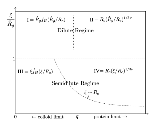
Figure 1: Different regimes for the depletion thickness in terms of $\xi/\hat{R}_{g}$ and $q=\hat{R}_{g}/R_{c}$. The functions $f_{H}(\hat{R}_{g}/R_{c})$ and $\hat{f}_{H}(\xi/R_{c})$ have a regular expansion in powers of their argument.

To conclude, let us summarize the different types of behavior of the depletion thickness in the $\xi$-$q$ diagram for the good-solvent case. They depend on the relative size of the three different scales that appear in the problem: the radius of gyration of the polymer, the radius of the colloid and the correlation length $\xi$. In the colloid regime in which $q<1$, i.e. $R_{c}>\hat{R}_{g}$, depletion shows two different behaviors, depending on the ratio $\xi/\hat{R}_{g}$. In the dilute regime in which the relevant scale is the radius of gyration (domain I in Fig. 1), $\delta_{s}$ is of order $\hat{R}_{g}$ with a proportionality constant that can be expanded in powers of $q$ (Helfrich expansion). If instead $\xi\ll\hat{R}_{g}$ (semidilute regime, domain III in Fig. 1), the relevant scale is the correlation length $\xi$. The depletion thickness is proportional to $\xi\sim\hat{R}_{g}\Phi^{-0.770}$ with a proportionality constant that admits an expansion in powers of $\xi/R_{c}$. Since $\xi\to 0$ for $\Phi\to\infty$, the limiting behavior is independent of the colloid radius. In the protein regime in which $q>1$, i.e., $R_{c}<\hat{R}_{g}$, depletion shows three different behaviors. In the dilute regime (domain II in Fig. 1), $\delta_{s}\sim R_{c}q^{1/(3\nu)}\sim R_{c}^{1-1/(3\nu)}\hat{R}_{g}^{1/(3\nu)}$, i.e., $\delta_{s}$ is much larger than the colloid radius but much smaller than $\hat{R}_{g}$. In the semidilute regime, two different behaviors occur. If $R_{c}\ll\xi\ll\hat{R}_{g}$ (domain IV), the role of the radius of gyration is now assumed by the correlation length and we have $\delta_{s}\sim R_{c}^{1-1/(3\nu)}\xi^{1/(3\nu)}$. Finally, as $\Phi$ increases further, one finally finds $\xi\ll R_{c}$ and one observes again $\delta_{s}\sim\xi$ (domain III).

The surface tension $\gamma$ was also computed in the PRISM approach FS-01 , obtaining

$$\beta\gamma=1.279\rho_{p}\hat{R}_{g}[1+1.06\Phi+0.634q].$$ (59)

Such an expression does not have the correct behavior for $q\to\infty$ or $\Phi\to\infty$. In the dilute regime and for small $q$, comparison with the field-theoretical results (we shall show that they are quite accurate) shows that it only provides a very rough approximation, differences being of order 20-30%.

The adsorption $\Gamma$ was computed numerically for the planar case ($q=0$) in Ref. LBMH-02-a , obtaining

$$\Gamma=-1.074\rho_{p}\hat{R}_{g}\left(1+7.63\Phi+14.56\Phi^{3}\right)^{-0.2565}.$$ (60)

This expression allows us to compute $\gamma$ for $q=0$ using the expression of the compressibility factor given in Ref. Pelissetto-08 . In the small-density limit we obtain

$$\beta\gamma=1.074\rho_{p}\hat{R}_{g}\left[1+0.334\Phi+O(\Phi^{2})\right],$$ (61)

while for $\Phi\to\infty$ we obtain

$$\beta\gamma=1.30\rho_{p}\hat{R}_{g}\Phi^{0.54}.$$ (62)

We can compare these expressions with the field-theory results. The leading density correction in Eq. (61) is approximately one half of that predicted by field theory, see Eq. (44), while the large-$\Phi$ expression (62) predicts a surface tension that is 17% smaller than Eq. (49).

Finally, we mention the phenomenological expression for the depletion thickness of Fleer et al. FST-07 ; FT-08

$${\delta_{s}\over R_{c}}=0.865q^{0.88}\left(1+3.95\Phi^{1.54}\right)^{-0.44},$$ (63)

which should be only valid in an intermediate range of values of $q$ FST-07 ; LT-11 , since it does not have the correct behavior in the limits $q\to 0$ and $q\to\infty$.

There are no predictions for polymers in the thermal crossover region. In this case, a new scale comes in, the dimension $R_{T}$ of the so-called thermal blob deGennes-79 . On scales $r\ll R_{T}$, the polymer behaves as an ideal chain, hence for $R_{c}\ll R_{T}$ the surface tension should coincide with that appropriate for an ideal chain. This implies that for any finite value of $z$ we should recover the ideal result for the surface tension, provided that $q$ is large enough. In particular, we predict

$$\beta\gamma=\rho_{p}R_{c}q^{2}$$ (64)

for all finite values of $z$ and $q\to\infty$. In practice, Eq. (42) holds also for finite $z$, with the values appropriate for the ideal chain, $\nu=1/2$ and $A_{\gamma,\infty}=1$. If instead $R_{c}\mathrel{\hbox to0.0pt{\lower 3.0pt\hbox{$\mathchar 536\relax$}\hss}\raise 2.0pt\hbox{$\mathchar 318\relax$}}R_{T}$, we expect to observe a nontrivial crossover behavior. Its determination is one of the purposes of the present paper.

III Polymer model and crossover behavior

In order to determine full-monomer properties, we consider the three-dimensional lattice Domb-Joyce model DJ-72 . We consider $N_{p}$ chains of $L$ monomers each on a finite cubic lattice of linear size $M$ with periodic boundary conditions. Each polymer chain is modeled by a random walk $\{{\mathbf{r}}_{1}^{(i)},\ldots,{\mathbf{r}}_{L}^{(i)}\}$ with $|{\mathbf{r}}_{\alpha}^{(i)}-{\mathbf{r}}_{\alpha+1}^{(i)}|=1$ (we take the lattice spacing as unit of length) and $1\leq i\leq N_{p}$. The Hamiltonian is given by

$$H=\sum_{i=1}^{N_{p}}\sum_{1\leq\alpha<\beta\leq L}\delta({\mathbf{r}}_{\alpha}^{(i)},{\mathbf{r}}_{\beta}^{(i)})+\sum_{1\leq i<j\leq N_{p}}\sum_{\alpha=1}^{L}\sum_{\beta=1}^{L}\delta({\mathbf{r}}_{\alpha}^{(i)},{\mathbf{r}}_{\beta}^{(j)}),$$ (65)

where $\delta({\mathbf{r}},{\mathbf{s}})$ is the Kronecker delta. Each configuration is weighted by $e^{-wH}$, where $w>0$ is a free parameter that plays the role of inverse temperature. This model is similar to the standard lattice self-avoiding walk (SAW) model, which is obtained in the limit $w\to+\infty$. For any positive $w$, this model has the same scaling limit as the SAW model DJ-72 and thus allows us to compute the universal scaling functions that are relevant for polymer solutions under good-solvent conditions. In the absence of colloids, there is a significant advantage in using Domb-Joyce chains instead of SAWs. For SAWs scaling corrections that decay as $L^{-\Delta}$ ($\Delta=0.528(12)$, Ref. Clisby-10 ) are particularly strong, hence the universal, large–degree-of-polymerization limit is only observed for quite large values of $L$. Finite-density properties are those that are mostly affected by scaling corrections, and indeed it is very difficult to determine universal thermodynamic properties of polymer solutions for $\Phi\mathrel{\hbox to0.0pt{\lower 3.0pt\hbox{$\mathchar 536\relax$}\hss}\raise 2.0pt\hbox{$\mathchar 318\relax$}}5$ by using lattice SAWs Pelissetto-08 . These difficulties are overcome by using the Domb-Joyce model for a particular value of $w$ BN-97 ; CMP-08 , $w=0.505838$. For this value of the repulsion parameter, the leading scaling corrections have a negligible amplitude BN-97 ; CMP-08 , so that scaling corrections decay faster, approximately as $1/L$. As a consequence, scaling results are obtained by using significantly shorter chains. Unfortunately, in the presence of a repulsive surface, new renormalization-group operators arise, which are associated with the surface DDE-83 . The leading one gives rise to corrections that scale as $L^{-\nu}$ DDE-83 , where $\nu$ is the Flory exponent (an explicit test of this prediction is presented in the supplementary material), hence it spoils somewhat the nice scaling behavior observed in the absence of colloids. Nonetheless, the Domb-Joyce model is still very convenient from a computational point of view. Since interactions are soft, the Monte Carlo dynamics for Domb-Joyce chains is much faster than for SAWs. We shall use the algorithm described in Ref. Pelissetto-08 , which allows one to obtain precise results for quite long chains ($L\mathrel{\hbox to0.0pt{\lower 3.0pt\hbox{$\mathchar 536\relax$}\hss}\raise 2.0pt\hbox{$\mathchar 318\relax$}}1000$) deep in the semidilute regime.

The Domb-Joyce model can also be used to derive the crossover functions that parametrize the crossover between the good-solvent and $\theta$-point regimes, at least not too close to the $\theta$ point, see Refs. CMP-08 ; DPP-thermal for a discussion. Indeed, if one neglects tricritical effects, which are only relevant close to the $\theta$ point Duplantier , this crossover can be parametrized by using the two-parameter model dCJ-book ; Schaefer-99 ; Sokal-94 . Two-parameter-model results are obtained BD-79 by taking the limit $w\to 0$, $L\to\infty$ at fixed $x=wL^{1/2}$. The variable $x$ interpolates between the ideal-chain limit ($x=0$) and the good-solvent limit ($x=\infty$). Indeed, for $w=0$ the Domb-Joyce model is simply the random-walk model, while for any $w\not=0$ and $L\to\infty$ one always obtains the good-solvent scaling behavior. The variable $x$ is proportional to the variable $z$ that is used in the context of the two-parameter model. We normalize $z$ as in Refs. CMP-08 ; DPP-thermal , setting

$$z\equiv\left({3\over 2\pi}\right)^{3/2}wL^{1/2}.$$ (66)

Note that the crossover can be equivalently parametrized Nickel-91 ; BN-97 ; PH-05 ; CMP-08 ; DPP-thermal by using the second-virial combination $A_{2,pp}=B_{2,pp}\hat{R}_{g}^{-3}$ ($\hat{R}_{g}$ is the zero-density radius of gyration), which varies between the good-solvent value CMP-06 $A_{2,pp}=5.500(3)$ and $A_{2,pp}=0$ at the $\theta$ point. With normalization (66) we have $A_{2,pp}(z)\approx 4\pi^{3/2}z$ for small $z$ BD-79 ; BN-97 . The correspondence between $A_{2,pp}$ and $z$ in the whole crossover region is given in Ref. CMP-08 .

As discussed in Ref. CMP-08 , the two-parameter-model results can be obtained from Monte Carlo simulations of the Domb-Joyce model by properly extrapolating the numerical results to $L\to\infty$. For each $z$ we consider several chain lengths $L_{i}$. For each of them we determine the interaction parameter $w_{i}$ by using Eq. (66), that is we set $w_{i}=(2\pi/3)^{3/2}zL_{i}^{-1/2}$. Simulations of chains of $L_{i}$ monomers are then performed setting $w=w_{i}$. Simulation results are then extrapolated to $L\to\infty$, taking into account that corrections are of order $1/\sqrt{L}$ BD-79 ; BN-97 .

In this paper we have performed a detailed study of the depletion for two values of $z$: $z=z^{(1)}=0.056215$ and $z=z^{(3)}=0.321650$, which correspond to CMP-08 $A_{2,pp}(z^{(1)})=0.9926(10)$ and $A_{2,pp}(z^{(3)})=2.9621(27)$. They correspond to polymer solutions of intermediate quality. Since $A_{2,pp}\approx 5.50$ CMP-06 under good-solvent conditions, we have $A_{2,pp}(z)/A_{2,pp}(z=\infty)=0.18$ and 0.54 for $z=z^{(1)}$ and $z^{(3)}$, respectively. Hence, for $z=z^{(1)}$ we are quite close to the $\theta$ point, while $z=z^{(3)}$ is intermediate between the good-solvent and $\theta$ regimes.

In this paper we discuss depletion effects close to neutral colloids, which are modelled as hard spheres that can move everywhere in space: their centers are not constrained to belong to a lattice point. This choice is particularly convenient since it drastically reduces lattice oscillations in colloid-polymer correlation functions. Such oscillations are instead present if colloids are required to sit on lattice points, as was done in Ref. PH-06 . Colloids and monomers interact by means of a simple exclusion potential. If ${\bf r}_{c}$ and ${\bf r}_{m}$ are the coordinates of a monomer and of a colloid, we take as interaction potential

$$U=+\infty \qquad|{\bf r}_{c}-{\bf r}_{m}|\leq R_{c},$$ (67)

$$U=0 \qquad|{\bf r}_{c}-{\bf r}_{m}|>R_{c}.$$ (68)

IV Dilute behavior

As we have seen in Sec. II.3, the low-density behavior of the surface tension or, equivalently, of the depletion thickness can be obtained by computing the virial coefficients $B_{2,cp}$ and $B_{3,cpp}$. We will thus report the computation of these two quantities and also of $B_{3,ccp}$, which would be relevant to characterize the effective interaction between two colloids in a dilute solution of polymers. Then, we shall discuss the depletion thickness $\delta_{s}$ for $\Phi=0$ and its first density correction.

IV.1 Virial coefficients

Table 1: Estimates of the universal surface combinations $R_{1,p}$ and $R_{2,p}$. We report full-monomer (FM) and single-blob (SB) results (see Sec. VI).

$z$	$R_{1,p}$ (FM)	$R_{2,p}$ (FM)	$R_{1,p}$ (SB)	$R_{2,p}$ (SB)
$\infty$	1.0605(3)	$-4.50(5)$	1.0514(2)	$-$4.44(1)
$z_{3}$	1.1066(1)	$-2.366(7)$	1.1065(3)	$-$2.387(8)
$z_{1}$	1.1221(4)	$-0.765(3)$	1.1222(3)	$-$0.771(4)

To determine the virial coefficients under good-solvent conditions we have simulated the Domb-Joyce model at $w=0.505838$. We consider chains of length $L=240,600,2400$ for $q\leq 3$, and $L=6000$, 24000 to derive the results corresponding to $4\leq q\leq 50$. Long chains are needed for large values of $q$ to ensure that the colloid radius is somewhat larger than the lattice spacing. Virial coefficients are determined as explained in App. A. The universal extrapolations of the finite-$L$ results for the adimensional combinations $A_{2,cp}=B_{2,cp}\hat{R}_{g}^{-3}$ and $A_{3,\#}=B_{3,\#}\hat{R}_{g}^{-6}$ are explicitly reported in the supplementary material. In the case of the two-parameter model, we have considered $L=120,240,600,1200,2400$ for $q\leq 3$ (for both $z=z^{(1)}$ and $z=z^{(3)}$) and $L=6000$, 30000 for $4\leq q\leq 30$ (only for $z=z^{(1)}$). The results at the same value of $z$ have then been extrapolated taking into account the $L^{-1/2}$ scaling corrections. Results are reported in the supplementary material. We also computed the adimensional combinations $R_{1,p}=P_{1,p}\hat{R}_{g}^{-1}$ and $R_{2,p}=P_{2,p}\hat{R}_{g}^{-4}$, which parametrize the depletion thickness in the presence of an impenetrable planar surface, see Table 1. The behavior of the adimensional combinations for $q\to 0$ is discussed in detail in Appendix B. We have

$$A_{2,cp} \approx {4\pi\over 3q^{3}}+{4\pi\over q^{2}}R_{1,p},$$ (69)

$$A_{3,cpp} \approx {8\pi\over 3q^{3}}A_{2,pp}+{4\pi\over q^{2}}\left(2A_{2,pp}R_{1,p}+R_{2,pp}\right),$$ (70)

$$A_{3,ccp} \approx {16\pi^{2}\over 9q^{6}}.$$ (71)

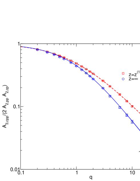
Figure 2: Combination ${A_{3,cpp}/(2A_{2,cp}A_{2,pp})}$ vs $q$. For $q\to 0$, such a combination converges to 1 for all values of $z$. We also report the approximate large-$q$ behavior.

For large values of $q$, we have $A_{2,cp}\sim q^{1/\nu-3}$, a behavior which can be derived by means of a blob argument PH-06 or from the large-$q$ behavior of $\gamma$, as discussed in Sec. II.4. More precisely, we predict $A_{2,cp}=4\pi A_{\gamma,\infty}q^{1/\nu-3}$, where $A_{\gamma,\infty}$ is the constant parametrizing the large-$q$ behavior of $\gamma$, defined by Eq. (42). Note that this relation holds both in the good-solvent regime with $\nu\approx 0.5876$ and in the crossover regime with $\nu=1/2$. As for the third virial coefficient $B_{3,cpp}$, we have already shown that $B_{3,cpp}/B_{2,cp}$ vanishes as $q\to\infty$. Hence, we expect

$${A_{3,cpp}\over A_{2,cp}}\sim q^{-\alpha},$$ (72)

with $\alpha>0$ for $q\to\infty$. We have been unable to predict the value of $\alpha$. A numerical fit of the data indicates $\alpha\approx 1$, both in the good-solvent limit and in the crossover region, see Fig. 2. As for $A_{3,ccp}$, a blob argument implies $A_{3,ccp}\sim q^{1/\nu-6}$.

Since knowledge of the virial coefficients for all values of $q$ allows us to have a complete control of the depletion effects in the dilute regime, it is useful to determine interpolations of the data, with the correct limiting behavior for $q\to 0$ and $q\to\infty$. We parametrize the data as

$$A_{2,cp} = \frac{4\pi}{3q^{3}}\left[\frac{1+a_{1}q+a_{2}q^{2}+a_{3}q^{3}}{1+a_{4}q}\right]^{1/(2\nu)},$$ (73)

$$A_{3,cpp} = \frac{8\pi A_{2,pp}}{3q^{3}}\left[\frac{1+a_{1}q+a_{2}q^{2}}{1+a_{3}q}\right]^{\beta},$$ (74)

$$A_{3,ccp} = \left(\frac{4\pi}{3q^{3}}\right)^{2}(1+a_{1}q+a_{2}q^{2}+\dots+a_{n}q^{n})^{1/(n\nu)},$$ (75)

We enforce the asymptotic behaviors (69), (70), and (71) for $q\to 0$. In the case of $A_{2,cp}$ and $A_{3,ccp}$ we have chosen the parametrization so to obtain the correct large-$q$ behaviors $A_{2,cp}\sim q^{1/\nu-3}$ and $A_{3,ccp}\sim q^{1/\nu-6}$ ($\nu=0.5876$ for the good-solvent case and $\nu=1/2$ for $z=z^{(1)}$ and $z^{(3)}$). In the case of $A_{3,cpp}$, $\beta$ is a free parameter. Fitting the data, we estimate the constants $a_{i}$. They are reported in Table 2.

Table 2: Coefficients parametrizing the universal virial combinations. For $A_{3,ccp}$ we use $n=3$ for $z=\infty$ and $z^{(3)}$, and $n=4$ for $z=z^{(1)}$. The interpolation is accurate in the range $0\leq q\leq q_{\rm max}$ in which we have data.

	$z$	$a_{1}$	$a_{2}$	$a_{3}$	$a_{4}$	$\beta$	$q_{\rm max}$
$A_{2,cp}$	$\infty$	4.1329	5.4906	2.12578	0.3942		50
	$z_{3}$	3.4774	3.37453	0.39752	0.15763		3
	$z_{1}$	3.4378	3.18934	0.20253	0.071526		30
$A_{3,ccp}$	$\infty$	12.9575	39.2297	152.514			$10$
	$z_{3}$	7.66551	55.4536	43.4239			$3$
	$z_{1}$	23.1533	0.0000	421.593	100.977		$6$
$A_{3,cpp}$	$\infty$	4.0850	5.0910	0.296425		0.51574	$20$
	$z^{(3)}$	3.36452	3.0418	1.3236		1.040	$3$
	$z^{(1)}$	2.55348	1.2711	0.42515		1.038	$30$

Using parametrization (73), we can compute the large-$q$ behavior of $A_{2,cp}$. In the good-solvent case we obtain $A_{2,cp}\approx 17.57q^{1/\nu-3}$. Since $A_{2,cp}=4\pi A_{\gamma,\infty}q^{1/\nu-3}$, we can estimate the constant $A_{\gamma,\infty}$ which appears in Eq. (42). We obtain $A_{\gamma,\infty}\approx 1.40$, which is in excellent agreement with the field-theoretical estimate 1.41 of Ref. HED-99 . For $z=z^{(1)}$ we obtain instead $A_{2,cp}\approx 11.9/q$. Since $A_{2,cp}=4\pi A_{\gamma,\infty}/q$ we obtain $A_{\gamma,\infty}=0.94$, which is close to the prediction $A_{\gamma,\infty}=1$ of Sec. II.4.

IV.2 Zero-density depletion thickness

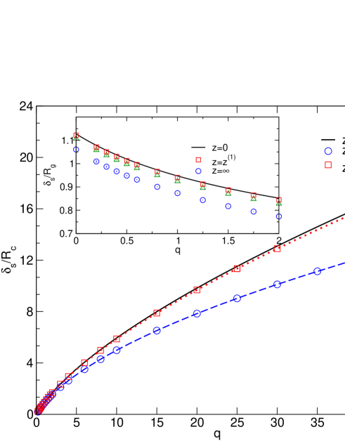
Figure 3: Depletion thickness ratio $\delta_{s}/R_{c}$ vs $q$ for $q\leq 40$ and $\Phi=0$. In the inset we report $\delta_{s}/\hat{R}_{g}$ in the interval $0\leq q\leq 2$. The dotted and dashed lines that go through the points in the main panel are obtained by using interpolation (73).

Knowledge of $A_{2,cp}$ allows us to compute the depletion thickness in the zero-density limit by using Eq. (36). In Fig. 3 we report our results. For $q\mathrel{\hbox to0.0pt{\lower 3.0pt\hbox{$\mathchar 536\relax$}\hss}\raise 2.0pt\hbox{$\mathchar 316\relax$}}2$, $\delta_{s}/\hat{R}_{g}$ has a tiny dependence on $z$: It slightly increases as $z$ decreases, and for $z=z^{(3)}$ and $z=z^{(1)}$ it is very close to the ideal-case result. For the surface case, these small differences can be appreciated by looking at the results given in Table 1, since $\delta_{s}/\hat{R}_{g}=R_{1,p}$ ($\delta_{s}/\hat{R}_{g}=1.128$ for $z=0$). The approximate independence of $\delta_{s}/\hat{R}_{g}$ on $z$ implies that the $z$-dependence of $\delta_{s}$ and of $\hat{R}_{g}$ are approximately the same: When $q$ is small, depletion effects are simply proportional to the typical size of the polymer and do not depend significantly on the quality of the solution. These considerations are valid only for $q$ not too large. For large values of $q$, significant differences between the good-solvent and the finite-$z$ case are observed, since the depletion thickness has a different asymptotic behavior for $q\to\infty$. Indeed, while $\delta_{s}/R_{c}\sim q^{2/3}$ for any finite $z$ as discussed in Sec. II.4, we have $\delta_{s}/R_{c}\sim q^{1/3\nu}\sim q^{0.567}$ in the good-solvent case.

To obtain a more quantitative comparison in the colloid regime, we can determine the small-$q$ behavior of $\delta_{s}(z)/\hat{R}_{g}$ by expanding parametrization (73) in powers of $q$. We obtain

$$\frac{\delta_{s}(\infty)}{\hat{R}_{g}} = 1.0605-0.281q+0.140q^{2}+\dots$$ (76)

$$\frac{\delta_{s}(z^{(3)})}{\hat{R}_{g}} = 1.107-0.274q+0.138q^{2}+\dots$$ (77)

$$\frac{\delta_{s}(z^{(1)})}{\hat{R}_{g}} = 1.122-0.276q+0.146q^{2}+\dots$$ (78)

$$\frac{\delta_{s}(0)}{\hat{R}_{g}} = 1.128-0.273q+0.138q^{2}+\dots$$ (79)

Results for $z=z^{(1)}$ cannot be distinguished from the ideal ones. Also the results for $z=z^{(3)}$ are very close to those corresponding to $z=0$. Slightly larger differences are observed for the good-solvent case.

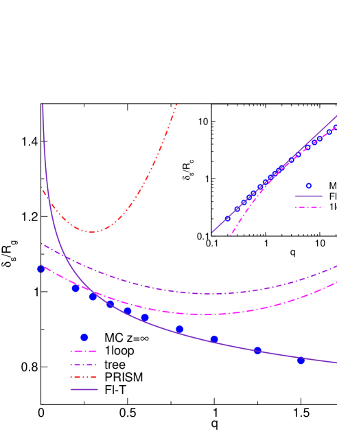
Figure 4: Comparison of the variour predictions for the depletion thickness at zero density in the good-solvent regime. We report the Monte Carlo estimates of $\delta_{s}/\hat{R}_{g}$ and (inset) $\delta_{s}/{R}_{c}$ versus $q$. We also report: the PRISM prediction obtained by using Eq. (59) (PRISM), Eq. (63) (Fl-T), the field-theoretical Helfrich expansions at tree level (tree) and at one loop (1loop), Eq. (80). In the inset we report (Fl-T) Eq. (63) and the large-$q$ field-theory prediction $\delta_{s}/R_{c}=1.62q^{0.567}$ (1loop).

In the good-solvent case, we can compare our estimates of $\delta_{s}$ with the field-theoretical predictions HED-99 ; MEB-01 . For small values of $q$ we report the tree-level result, which can be derived from Eq. (44), and the one-loop result obtained from Eq. (41):

$$\left(\frac{\delta_{s}}{\hat{R}_{g}}\right)_{\rm tree}=1.13-0.27q+\dots$$

$$\left(\frac{\delta_{s}}{\hat{R}_{g}}\right)_{\rm 1loop}=1.07q-0.28q^{2}+0.18q^{3}+\dots$$ (80)

Comparison with the Monte Carlo prediction (76) shows that differences are tiny. Moreover, it is very reassuring that loop corrections correctly change the values of the Helfrich coefficients towards the numerically determined values. For large values of $q$, we have $\delta_{s}/R_{c}\approx(3A_{\gamma,\infty}q^{1/\nu})^{1/3}$. The Monte Carlo results imply $\delta_{s}/R_{c}\approx 1.61q^{1/(3\nu)}$, while field theory predicts $\delta_{s}/R_{c}\approx 1.62q^{1/(3\nu)}$. Again, field theory appears to work very nicely. Other predictions are compared in Fig. 4. As already discussed, Eq. (59) gives only a very rough approximation that fails completely for $q\mathrel{\hbox to0.0pt{\lower 3.0pt\hbox{$\mathchar 536\relax$}\hss}\raise 2.0pt\hbox{$\mathchar 318\relax$}}0.7$. The phenomenological expression (63), instead, provides a quite good approximation in a quite large intermediate range, from $q\approx 0.2$ up to $q\approx 4$. The approximation fails in the planar limit—it predicts $\delta_{s}=\infty$ for $q\to 0$—and for large values of $q$, as it predicts $\delta_{s}\sim q^{0.88}$, while the correct behavior is $\delta_{s}\sim q^{0.567}$.

IV.3 Density correction to the depletion thickness

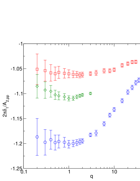
Figure 5: Density-correction combination $2\pi\delta_{1}(q)/A_{2,pp}$ versus $q$ for $z=z^{(1)}$, $z^{(3)}$ and the good-solvent case $z=\infty$. For $q=0$, $2\pi\delta_{1}(q)/A_{2,pp}=-1.030(4)$, $-$1.083(3), $-$1.16(2) for the same values of $z$.

Knowledge of the third virial coefficient $A_{3,cpp}$ allows one to determine the first density correction to $\delta_{s}(q,\Phi)$, see Eq. (36). We define

$${\delta_{s}(q,\Phi)\over\delta_{s}(q,0)}=1+\delta_{1}(q)\Phi+O(\Phi^{2}).$$ (81)

For $q\to\infty$, since $A_{3,cpp}/A_{2,cp}\to 0$ in this limit, Eq. (36) implies $\delta_{1}(q)\to-A_{2,pp}/(2\pi)$. In Fig. 5 we report the combination $2\pi\delta_{1}(q)/A_{2,pp}$, which converges to $-1$ for $q\to\infty$ and any value of $z$. It is evident that there are two different regimes. For $q$ not too large—$q\mathrel{\hbox to0.0pt{\lower 3.0pt\hbox{$\mathchar 536\relax$}\hss}\raise 2.0pt\hbox{$\mathchar 316\relax$}}2$ and $q\mathrel{\hbox to0.0pt{\lower 3.0pt\hbox{$\mathchar 536\relax$}\hss}\raise 2.0pt\hbox{$\mathchar 316\relax$}}10$ for the good-solvent case and for $z=z^{(1)}$, respectively—the density correction is mostly independent of $q$. In the opposite limit ($q$ large), a more pronounced $q$ dependence is observed, related to the fact that $2\pi\delta_{1}(q)/A_{2,pp}$ always converges to $-1$ as $q\to\infty$. The $z$ dependence of the combination $2\pi\delta_{1}(q)/A_{2,pp}$ is not large: it changes by at most 5% as $z$ increases from $z^{(1)}$ to $z^{(3)}$ and by 10% at most from $z^{(3)}$ to $\infty$ (the good-solvent case). Hence, a rough approximation for $\delta_{1}(q)$ is simply $\delta_{1}(q)=-A_{2,pp}/2\pi$, which relates directly solution quality to depletion effects. The quality of this approximation improves as $z$ decreases.

We can compare our good-solvent results with several predictions that hold for small values of $q$. Field theory MEB-01 , see Eq. (44), gives

$$\delta_{1}(q)=-1.23-0.015q+\ldots$$ (82)

The value for $q=0$ is not far from the numerical estimate $\delta_{1}(0)=3R_{2,pp}/(4\pi R_{1,p})=-1.013(14)$, indicating that the renormalized tree-level approximation reasonably predicts the low-density behavior in the colloid regime. Moreover, the leading $q$ correction is negative and very small, in agreement with our results: the $q$ dependence of $\delta_{1}(q)$ is tiny for $q\to 0$.

For $q=0$, we can also use the PRISM prediction (59) and the numerical expression (60) for $\Gamma$ of Ref. LBMH-02-a . We obtain in the two cases $\delta_{1}(0)=-0.51$ and $-1.96$, respectively. None of the two expressions appears to provide an accurate estimate of $\delta_{1}(q)$ for $q=0$.

V Finite-density results

V.1 Numerical determination of $G_{cp}$

Let us now determine the depletion behavior at finite polymer density. For this purpose we perform finite-density simulations of the Domb-Joyce model in a cubic box in the presence of a single colloid and compute the density profile $\rho_{\rm mon}(r)$, which gives the density of monomers at distance $r$ from the colloid, and the analogous density $\rho_{CM}(r)$, which gives the density of polymer centers of mass. To compute $g_{{\rm mon},cp}(r)$ and $g_{CM,cp}(r)$ we should determine first the bulk polymer (or monomer) density. We proceed as follows. If the cubic box of volume $V=M^{3}$ contains $N_{p}$ polymers of $L$ monomers each, for each distance $\Lambda<M/2$ we define an effective bulk monomer density

$$\rho_{{\rm mon},b}(\Lambda)={1\over V-V_{\Lambda}}\left(LN_{p}-\int_{r\leq\Lambda}d{\bf r}\,\rho_{\rm mon}(r)\right),$$ (83)

where $V_{\Lambda}={4\pi\over 3}\Lambda^{3}$. The quantity $\rho_{{\rm mon},b}(\Lambda)$ gives the average monomer density outside a sphere of radius $\Lambda$ centered on the colloid. As a function of $\Lambda$, $\rho_{{\rm mon},b}(\Lambda)$ first increases, then shows an approximate plateau, and finally shows a systematic upward or downward drift with a large statistical error. We take the approximately constant value of $\rho_{\rm mon}(\Lambda)$ in the plateau as an estimate of the bulk monomer density. Then, we estimate $g_{{\rm mon},cp}(r)=\rho_{\rm mon}(r)/\rho_{{\rm mon},b}(\Lambda)$ and

$$G_{cp}=\int_{r\leq\Lambda}d{\bf r}\,\left(g_{{\rm mon},cp}(r)-1\right).$$ (84)

The same calculation, mutatis mutandis, has been performed for the colloid polymer–center-of-mass distribution function.

As a check, we computed $G_{cp}$ by using a third method. If $\hat{g}_{{\rm mon},cp}({\bf k})$ is the Fourier transform of the pair distribution function, the integral $G_{cp}$ can be computed as

$$G_{cp}=\lim_{k\to 0}\hat{g}_{{\rm mon},cp}({\bf k}).$$ (85)

Such a definition is much less sensitive to the definition of the bulk monomer density, but requires an extrapolation in $k$. Since we are considering a cubic box, it is natural to restrict the calculation to ${\bf k}=(k,0,0)$ (or to $(0,k,0)$ and $(0,0,k)$, which are equivalent by symmetry). For $k\not=0$ the function $\hat{g}_{{\rm mon},cp}({\bf k})$ admits an expansion in powers of $k^{2}$, i.e.

$$\hat{g}_{{\rm mon},cp}({\bf k})=G_{cp}+a_{1}k^{2}+a_{2}k^{4}+a_{3}k^{6}+\ldots$$ (86)

To estimate $G_{cp}$, we consider the smallest momenta available for a finite box of volume $V=M^{3}$, i.e., $k_{1}=2\pi/M$, $k_{2}=2k_{1}$, $k_{3}=3k_{1}$, $k_{4}=4k_{1}$, and the approximants

$$G_{cp}^{(1)} = {4\over 3}\hat{g}_{{\rm mon},cp}({\bf k}_{1})-{1\over 3}\hat{g}_{{\rm mon},cp}({\bf k}_{2}),$$ (87)

$$G_{cp}^{(2)} = {3\over 2}\hat{g}_{{\rm mon},cp}({\bf k}_{1})-{3\over 5}\hat{g}_{{\rm mon},cp}({\bf k}_{2})+{1\over 10}\hat{g}_{{\rm mon},cp}({\bf k}_{3}),$$

$$G_{cp}^{(3)} = {8\over 5}\hat{g}_{{\rm mon},cp}({\bf k}_{1})-{4\over 5}\hat{g}_{{\rm mon},cp}({\bf k}_{2})$$

$$+{8\over 35}\hat{g}_{{\rm mon},cp}({\bf k}_{3})-{1\over 35}\hat{g}_{{\rm mon},cp}({\bf k}_{4}).$$

Using Eq. (86), it is easy to show that $G_{cp}^{(n)}=G_{cp}+O(M^{-2n-2})$. Note that we do not consider the volume corrections (of order $1/V=M^{-3}$ see, e.g., Ref. LP-61 ), which affect $\hat{g}_{\rm mon}({\bf k})$ at fixed $k$. For the typical volumes we consider, such corrections are negligible (see Ref. DPP-thermal for the analogous discussion concerning the polymer-polymer distribution function). On the other hand, we observe a systematic difference between $G^{(1)}_{cp}$ and $G^{(2)}_{cp}$, while $G^{(2)}_{cp}\approx G^{(3)}_{cp}$ in all cases. Clearly, the $M^{-4}$ corrections that are present when considering $G^{(1)}_{cp}$ are not negligible. Therefore, we take $G^{(2)}_{cp}$ as the estimate of $G_{cp}$.

V.2 Colloid-monomer pair distribution functions

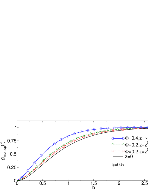
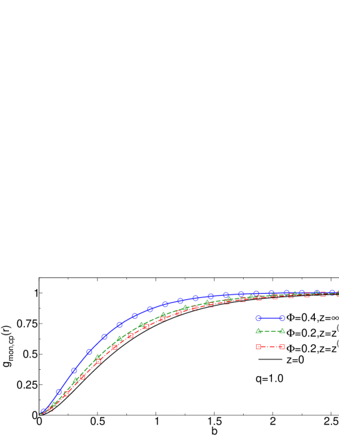
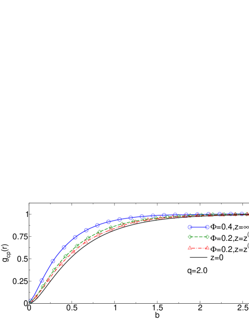
Figure 6: Pair distribution function $g_{{\rm mon},cp}(r)$ as a function of $b=(r-R_{c})/\hat{R}_{g}$ for different values of $q$, $z$, and $\Phi$ in the dilute regime. Eq. (88) is used for $z=0$.

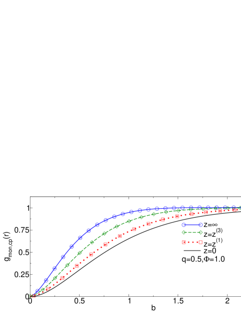
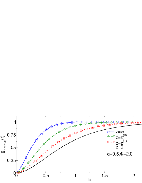
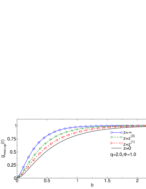
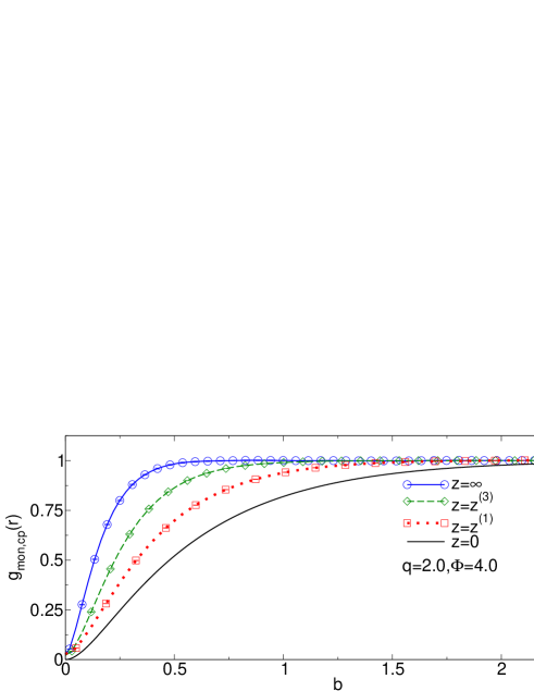
Figure 7: Pair distribution function $g_{{\rm mon},cp}(r)$ as a function of $b=(r-R_{c})/\hat{R}_{g}$ in the semidilute regime. Eq. (88) is used for $z=0$.

We study the solvation properties of a single colloid in the semidilute regime for $q=0.5$, 1 and 2, considering the good-solvent case and two values of $z$, $z=z^{(1)}$ and $z=z^{(3)}$, in the thermal crossover region. In each case we compute numerically the pair correlation functions $g_{{\rm mon},cp}(r)$, $g_{CM,cp}(r)$, and the Fourier transform $\hat{g}_{{\rm mon},cp}(k)$ for the values of $k$ that are relevant for the computation of the approximants (87) for a few values of $\Phi$, up to $\Phi=4$. We also present good-solvent results for the surface case ($q=0$) up to $\Phi=8$. In this case, however, we have only measured the monomer density profile close to the surface.

The function $g_{{\rm mon},cp}(r)$ is shown in Fig. 6 as a function of $b=(r-R_{c})/\hat{R}_{g}$ for the lowest values of $\Phi$ we have considered, together with expression EHD-96

$$g_{{\rm mon},cp}(r) = \frac{q^{2}b^{2}+2bq\psi(b/2)+f(b/2)}{\left(bq+1\right)^{2}},$$ (88)

$$f(x) = 2\psi(x)-\psi(2x),$$

$$\psi(x) = \hbox{erf}\,(x)+\frac{2x}{\sqrt{\pi}}e^{-x^{2}}-2x^{2}\hbox{erfc}\,(x),$$

which holds in the ideal case ($z=0$). Here $b=(r-R_{c})/\hat{R}_{g}$ is the distance from the colloid surface in units of $\hat{R}_{g}$, ${\rm erf}(x)$ is the error function and ${\rm erfc}(x)=1-{\rm erf}(x)$. For all values of $q$, the results for $z=z^{(1)}$ and, to a lesser extent, those for $z=z^{(3)}$ are very close to the ideal ones, indicating that in the dilute regime depletion effects for $q\leq 2$ are little sensitive to solution quality at least up to $z=z^{(3)}$, as already discussed in the zero-density limit. In Fig. 7 we show the same distribution function for larger values of $\Phi$. Depletion effects are much more dependent on solution quality and deviations from ideality are clearly visible, even for $z=z^{(1)}$.

V.3 Finite-density depletion thickness and adsorption

Table 3: Full-monomer estimates of the depletion thickness ratio $\delta_{s}(q,\Phi)/R_{c}$ for $z=z^{(1)}$: (a) is the estimate obtained by using extrapolation (87), (b) is the direct estimate obtained by using $g_{{\rm mon},cp}(r)$, and (c) is the direct estimate obtained by using $g_{CM,cp}(r)$. The last column gives the final estimate.

$q$	$\Phi$	(a)	(b)	(c)	final
0.5	0.2	0.48(2)	0.486(5)	0.490(3)	0.48(2)
	1.0	0.417(2)	0.440(2)	0.441(1)	0.428(14)
	2.0	0.383(2)	0.392(2)	0.390(2)	0.387(6)
1	0.2	0.900(6)	0.886(4)	0.905(4)	0.90(1)
	1.0	0.778(3)	0.81(1)	0.820(4)	0.80(2)
	4.0	0.641(3)	0.615(4)	0.610(5)	0.62(2)
2	0.2	1.7(1)	1.63(6)	1.66(2)	1.7(1)
	1.0	1.45(2)	1.44(1)	1.45(1)	1.45(2)
	4.0	1.080(5)	1.135(6)	1.151(8)	1.12(4)

Table 4: Full-monomer estimates of the depletion thickness raio $\delta_{s}(q,\Phi)/R_{c}$ for $z=z^{(3)}$: (a) is the estimate obtained by using extrapolation (87), (b) is the direct estimate obtained by using $g_{{\rm mon},cp}(r)$, and (c) is the direct estimate obtained by using $g_{CM,cp}(r)$. The last column gives the final estimate.

$q$	$\Phi$	(a)	(b)	(c)	final
0.5	0.2	0.45(1)	0.47(1)	0.466(5)	0.46(2)
	1.0	0.343(3)	0.338(2)	0.340(1)	0.340(6)
	2.0	0.2656(7)	0.269(2)	0.266(1)	0.268(3)
1	0.2	0.826(9)	0.842(15)	0.837(5)	0.84(2)
	1.0	0.634(5)	0.631(8)	0.636(4)	0.632(9)
	2.0	0.498(2)	0.47(2)	0.507(3)	0.503(7)
	4.0	0.3699(6)	0.38(1)	0.36(1)	0.365(15)
2	0.2	1.50(4)	1.51(5)	1.56(2)	1.52(6)
	1.0	1.15(1)	1.13(1)	1.134(8)	1.14(2)
	2.0	0.92(1)	0.96(2)	0.96(1)	0.94(3)
	4.0	0.498(2)	0.47(2)	0.507(3)	0.503(7)

Table 5: Full-monomer estimates of the depletion thickness ratio $\delta_{s}(q,\Phi)/R_{c}$ in the good-solvent case: (a) is the estimate obtained by using extrapolation (87), (b) is the direct estimate obtained by using $g_{{\rm mon},cp}(r)$, and (c) is the direct estimate obtained by using $g_{CM,cp}(r)$. The last column gives the final estimate. For $q=0.5$ and $\Phi=4.0$, the box was not large enough to allow us to estimate reliably $G_{cp}$ from $g_{CM,cp}(r)$.

$q$	$\Phi$	(a)	(b)	(c)	final
0.5	0.4	0.335(25)	0.340(5)	0.337(4)	0.335(25)
	1.0	0.239(6)	0.236(3)	0.236(2)	0.239(6)
	2.0	0.168(5)	0.162(4)	0.155(4)	0.162(11)
	4.0	0.110(2)	0.096(4)	—	0.102(10)
1	0.4	0.625(15)	0.615(3)	0.612(5)	0.624(17)
	1.0	0.439(8)	0.435(3)	0.427(3)	0.436(11)
	2.0	0.35(3)	0.313(8)	0.30(1)	0.335(45)
	4.0	0.195(6)	0.192(3)	0.168(7)	0.18(2)
2	0.4	1.07(5)	—	1.175(8)	1.10(8)
	1.0	0.79(3)	0.79(1)	0.78(1)	0.795(25)
	2.0	0.67(4)	0.58(1)	0.59(2)	0.65(8)
	4.0	0.39(2)	0.37(1)	0.34(3)	0.36(5)

Table 6: Depletion thickness ratio $\delta_{s}/\hat{R}_{g}$ in the presence of a surface ($q=0$) in the good-solvent regime. Direct estimates obtained by using the surface-monomer distribution function (monomer density profile).

$\Phi$	$\delta_{s}/\hat{R}_{g}$
0.3	0.820(1)
0.7	0.621(2)
1.0	0.545(6)
1.5	0.420(1)
2.0	0.352(1)
4.0	0.218(2)
6.0	0.162(3)
8.0	0.127(4)

By using the pair distribution function $g_{{\rm mon},cp}(r)$ we can compute the integral $G_{cp}$, as discussed in Sec. V.1, and the depletion thickness $\delta_{s}$. The results for $q\not=0$ are reported in Tables 3, 4, and 5 [estimates (b)], those for $q=0$ in Table 6. Errors take only into account statistical fluctuations, hence they should not be taken too seriously, as we shall discuss below. The same procedure can also be applied to $g_{CM,cp}(r)$. Although, this pair distribution function is quite different from $g_{{\rm mon},cp}(r)$ (it will be discussed in Sec. VI), the estimates of $G_{cp}$ it provides are close to those obtained by using $g_{{\rm mon},cp}(r)$, see estimates (c) reported in Tables 3, 4, and 5. In most of the cases, estimates (b) and (c) are consistent within errors. In a few cases, however—mostly for the largest values of $\Phi$—differences are observed, indicating that systematic errors are larger than statistical ones. To obtain a better control of systematic effects, it is important to have a different, conceptually independent method to estimate $G_{cp}$. For this purpose we compute $G_{cp}$ from the Fourier transform of the monomer distribution function. We use the method described in the previous section, and, in particular, the approximant $G^{(2)}_{cp}$ defined in Eq. (87). The corresponding results for $\delta_{s}$ are reported in Tables 3, 4, and 5 [estimates (a)]. For small values of $\Phi$, estimates (a) are consistent with the direct estimates (b) and (c). However, errors are significantly larger than those on (b) and (c), hence we cannot exclude that the direct estimates show systematic deviations which are larger than their statistical errors. For $\Phi\geq 1$, all estimates have comparable statistical errors, but results are sometimes not consistent. In order to quote a reliable estimate with a correct error bar, we take a conservative attitude. We determine the largest interval that contains estimates (a), (b) and (c) with their errors. The midpoint is the final estimate, while the half-width gives the error. The results of this procedure are reported (column “final”) in Tables 3, 4, and 5.

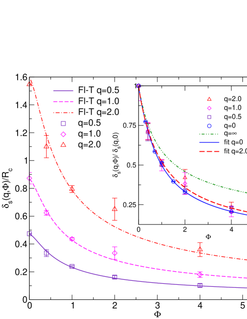
Figure 8: Main panel: Depletion thickness ratio $\delta_{s}(q,\Phi)/\hat{R}_{c}$ as a function of $\Phi$ in the good-solvent regime; we report the Monte Carlo data (points) and the phenomenological prediction (63) (lines, Fl-T). Inset: $\delta_{s}(q,\Phi)/\delta_{s}(q,0)$ as a function of $\Phi$; we report the data (points), the interpolations (90) (fit), and the curve $K_{p}(\Phi)^{-1/3}$ ($q=\infty$), see text for a discussion.

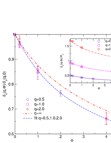
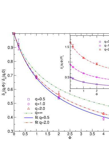
Figure 9: Plot of $\delta_{s}(q,\Phi)/\delta_{s}(q,0)$ as a function of $\Phi$ for $q=0.5,1,2$ for $z=z^{(1)}$ (top) and $z=z^{(3)}$ (bottom). Lines correspond to the interpolations (90) (fit), while the curve $q=\infty$ corresponds to $K_{p}(\Phi)^{-1/3}$, as discussed in the text. In the inset we report $\delta_{s}(q,\Phi)/\hat{R}_{c}$ (points) and the corresponding interpolations (lines). The function $K_{p}(\Phi)$ is obtained by using the equation of state reported in Ref. DPP-thermal .

The good-solvent results are shown in Fig. 8. The depletion thickness decreases very rapidly with $\Phi$. For instance, for $q=2$, we find $\delta_{s}/R_{c}=1.5305(5)$ for $\Phi=0$ and $\delta_{s}/R_{c}=1.10(6)$ for $\Phi=0.4$. Even a small increase of the polymer density significantly reduces the width of the depleted layer around the colloid. An interesting feature of the results is that the $\Phi$ dependence for $0\leq q\leq 2$, the interval of $q$ we investigate, is approximately independent of $q$. This is evident from the results reported in the inset of Fig. 8, where we show the ratio $\delta_{s}(q,\Phi)/\delta_{s}(q,0)$ as a function of $\Phi$. The $q$-dependence is practically absent. This result is far from obvious and is consistent with what we already observed in Sec. IV.3, where we pointed out that the first density correction is approximately $q$-independent for $q\mathrel{\hbox to0.0pt{\lower 3.0pt\hbox{$\mathchar 536\relax$}\hss}\raise 2.0pt\hbox{$\mathchar 316\relax$}}2$.

The $q$ independence of the ratio is not expected to hold much beyond $\Phi=4$, our largest density. Indeed, as we discussed in Sec. II.4, $\delta_{s}(q,\Phi)\sim\xi(\Phi)$ for $\Phi\to\infty$ and any $q$, so $\Delta(q,\Phi)=\delta_{s}(q,\Phi)/\delta_{s}(q,0)\sim\xi(\Phi)/\delta_{s}(q,0)$. Since $\delta_{s}(q,0)$ varies significantly with $q$, factorization breaks down deep in the semidilute regime (some differences are already observed for $\Phi=4$). Analogously, such a property does not hold for large values of $q$. Indeed, as long as $R_{c}\ll\xi$, Eq. (57) holds, which implies

$$\Delta(q,\Phi)={\delta_{s}(q,\Phi)\over\delta_{s}(q,0)}=K_{p}(\rho_{p})^{-1/3}.$$ (89)

Using the equation of state of Ref. Pelissetto-08 , we can compute $K_{p}(\rho_{p})$, hence $\Delta(q,\Phi)$ for $q\to\infty$. The corresponding curve is reported in Fig. 8 (line “$q=\infty$” in the inset). Differences with the Monte Carlo results are quite significant. For instance, for $\Phi=4$, Eq. (89) predicts $\Delta(q,4)=0.346$ for $q\to\infty$, to be compared with $\Delta(q,4)=0.232(5)$ and 0.23(3) for $q=0.5$ and $q=2$, respectively. Note that differences increase rapidly with $\Phi$. This is due to the fact that, for $q\leq 2$, $\Delta$ already scales as $\Phi^{-0.8}$ for $\Phi\mathrel{\hbox to0.0pt{\lower 3.0pt\hbox{$\mathchar 536\relax$}\hss}\raise 2.0pt\hbox{$\mathchar 318\relax$}}2$, while $\Delta\sim\Phi^{-0.437}$ for large values of $q$.

In Fig. 8 we also report the phenomenological approximation (63), which works quite well for $0.2\leq q\leq 4$ in the dilute limit. Also the density dependence is well reproduced for $0.5\leq q\leq 2$: Tiny differences are only observed in the dilute regime.

In Fig. 9 we report the depletion thickness in the thermal crossover region, for $z=z^{(1)}$ and $z=z^{(3)}$. The qualitative behavior is very similar to that observed in the good-solvent case. For all values of $q$ considered, the $\Phi$ dependence and the $q$ dependence appear to be factorized, i.e. $\delta_{s}(q,\Phi)/\delta_{s}(q,0)$ is essentially independent of $q$. Such a result is expected to hold in a $q$ interval that is larger than in the good-solvent case. First, we have already observed that the first density correction is essentially $q$ independent for $q\mathrel{\hbox to0.0pt{\lower 3.0pt\hbox{$\mathchar 536\relax$}\hss}\raise 2.0pt\hbox{$\mathchar 316\relax$}}10$ for $z=z^{(1)}$. Second, the difference between our data and the large-$q$ prediction (89), which should also hold in the thermal crossover region, decreases as $z$ decreases. Finally, it is interesting to observe that in the crossover region the density dependence of $\delta_{s}$ is smaller than in the good-solvent case. For $\Phi=4$, $\delta_{s}(q,4)/\delta_{s}(q,0)=0.22$, 0.40, 0.66, for $z=\infty$, $z=z^{(3)}$, and $z=z^{(1)}$. This result is of course expected, since $\delta_{s}$ becomes density independent for $z\to 0$.

Table 7: Coefficients parametrizing the depletion-thickness interpolations (90) as function of density. The parametrizations should hold for $\Phi\leq\Phi_{\rm max}$.

$z$	$q$	$n$	$a_{1}$	$a_{2}$	$a_{3}$	$\eta$	$\Phi_{\rm max}$
$\infty$	0	3	3.9467	4.3305	5.8889	0.770	$4$
	0.5	3	4.0909	6.8272	2.6728	0.770	$4$
	1.0	3	4.0987	4.4818	4.92968	0.770	$4$
	2.0	3	4.0753	6.12348	1.92624	0.770	$4$
$z^{(3)}$	0.5	2	1.8641	1.0753	0	0.5579	$2$
	1.0	2	1.8747	1.0279	0	0.5579	$4$
	2.0	2	2.0279	1.16915	0	0.5128	$4$
$z^{(1)}$	0.5/1.0/2.0	3	1.7682	1.8151	0.6591	0.2845	$4$

To summarize our results in a simple way, we determine interpolations of the Monte Carlo data for the depletion thickness. For this purpose we fit the results to

$${\delta_{s}(q,\Phi)\over\delta_{s}(q,0)}=\left(1+\sum_{k=1}^{n}a_{k}\Phi^{k}\right)^{-\eta/n}.$$ (90)

We set $n=2$ or $3$ and $a_{1}=-n\delta_{1}/\eta$, where $\delta_{1}$ is the first density correction defined in Eq. (81), in such a way to reproduce accurately the low-density behavior. In the good-solvent case, we have $\delta_{s}\sim\Phi^{-0.770}$ for $\Phi\to\infty$. We have enforced this condition in our interpolations, requiring $\eta=0.770$. In the crossover region, we do not have predictions for the large-$\Phi$ behavior, hence $\eta$ has been taken as a free parameter. For $z=z^{(3)}$ and $q=0.5$, our data extends only up to $\Phi=2$, hence fits are not very sensitive to $\eta$. To obtain stable fit results, we fix $\eta$ to be equal to the result obtained for $q=1$ and $z=z^{(3)}$. For the good-solvent case and for $z=z^{(3)}$ the results show a tiny $q$-dependence for $\Phi=4$, hence we determine an interpolation for each value of $q$. On the other hand, for $z=z^{(1)}$ results for different values of $q$ coincide within errors. Hence, we have performed a single fit, considering simultaneously all value of $q$. The coefficients of the interpolations are reported in Table 7. The interpolations are reported in Figs. 8 and 9.

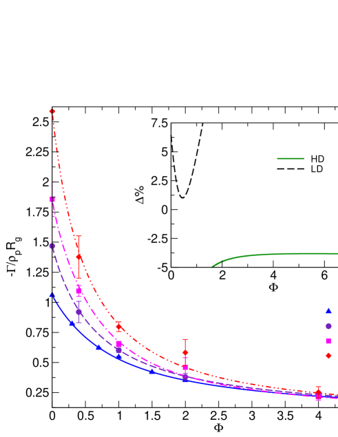
Figure 10: Main panel: Rescaled adsorption $\hat{\Gamma}=-\Gamma/(\rho_{p}\hat{R}_{g})$ as a function of $\Phi$ for $q=0,0.5,1.0,2.0$ as a function of $\Phi$ in the good-solvent regime; lines are obtained by using interpolations (90). In the inset we report the relative deviations $\Delta=100({\Gamma}_{\rm pred}/{\Gamma}_{MC}-1)$, where ${\Gamma}_{\rm pred}$ is either Eq. (53) (HD) or Eq. (91) (LD), and $\Gamma_{MC}$ is obtained by using interpolations (90).

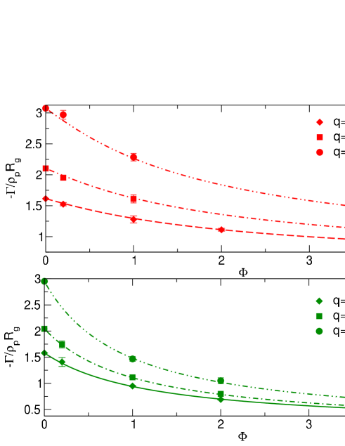
Figure 11: Rescaled adsorption $-\Gamma/(\rho_{p}\hat{R}_{g})$ as a function of $\Phi$ for $q=0.5,1,2$. We report data for $z=z^{(1)}$ (top) and $z=z^{(3)}$ (bottom). Lines are obtained by using interpolations (90).

Finally, we wish to compare our good-solvent data with the large-$\Phi$ field-theoretical predictions. In Fig. 10 we show our results for the adsorption $\Gamma$. As predicted by theory, adsorption becomes independent of $q$ as $\Phi$ increases. On the scale of the figure, all curves coincide for $\Phi\mathrel{\hbox to0.0pt{\lower 3.0pt\hbox{$\mathchar 536\relax$}\hss}\raise 2.0pt\hbox{$\mathchar 318\relax$}}4$. This is consistent with the results of Ref. LBMH-02-a , where it was shown that $\gamma(q,\Phi)/\gamma(0,\Phi)$ converges to 1 for large $\Phi$ for all $q\leq 1.68$. Note that this ratio becomes approximately 1 at densities which are significantly larger than $\Phi\approx 4$. This is due to the fact that $\beta\gamma(q,\Phi)$ is obtained by integrating $\Gamma(q,\Phi)$, see Eq. (5), from 0 to $\Phi$, hence including the dilute region in which depletion effects are strongly $q$-dependent. Quantitatively, the field-theoretical prediction (53), $\Gamma/(\rho_{p}\hat{R}_{g})\approx-0.649\Phi^{-0.770}$, holds quite precisely. For the surface case ($q=0$) it is in good agreement with our data for $\Phi\mathrel{\hbox to0.0pt{\lower 3.0pt\hbox{$\mathchar 536\relax$}\hss}\raise 2.0pt\hbox{$\mathchar 318\relax$}}2$ with deviations which are of order 4% (see inset). For instance, interpolation (90) gives $\Gamma/(\rho_{p}\hat{R}_{g})=-0.673\Phi^{-0.770}$, which is compatible with prediction (53). We can also compare our results with interpolation (60). For $\Phi\to\infty$ it predicts $\Gamma/(\rho_{p}\hat{R}_{g})=-0.54\Phi^{-0.770}$, which differs significantly from our result. This is probably related to the fact that Eq. (60) is obtained by fitting SAW data. Indeed, such a model shows large finite-length corrections to scaling, especially in the semidilute regime Pelissetto-08 . Hence, even the results obtained from simulations of rather long walks ($L\approx 10^{3}$) do not probe the universal, infinite-length behavior.

We can also compare the results with low-density prediction

$$-{\Gamma\over\rho_{p}\hat{R}_{g}} = {1.129(1+1.4\Phi)\over K_{p}(\rho_{p})},$$ (91)

where $K_{p}(\rho_{p})$ is obtained from the equation of state of Ref. Pelissetto-08 . Such an expression describes well the data up to $\Phi\approx 0.5$, with deviations of less than 6%.

VI Comparison with single-blob results

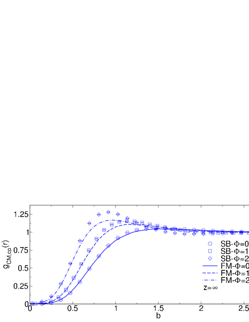
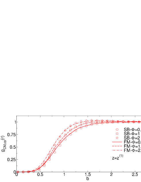
Figure 12: Pair distribution function $g_{CM,cp}(r)$ for $q=0.5$ as a function of $b=(r-R_{c})/\hat{R}_{g}$ under good-solvent conditions (top), and $z=z^{(1)}$ (bottom).

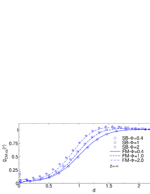
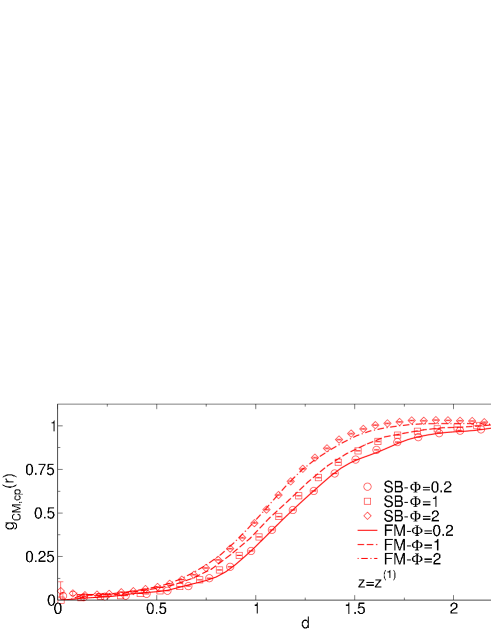
Figure 13: Pair distribution function $g_{CM,cp}(r)$ for $q=2$ as a function of $d=r/\hat{R}_{g}$ under good-solvent conditions (top), and $z=z^{(1)}$ (bottom).

Recently, there has been significant work dealing with coarse-grained models of polymer solutions MullerPlathe-02 ; PK-09 ; Voth2009 ; PCCP2009 ; SM2009 ; FarDisc2010 . The simplest model Likos-01 ; LBHM-00 ; HL-02 is obtained by representing polymers with monoatomic molecules (single-blob model) interacting via the polymer center-of-mass potential of mean force. By definition the model reproduces the dilute behavior of the solution, but fails to be accurate as soon as polymer-polymer overlaps become important, i.e. for $\Phi\mathrel{\hbox to0.0pt{\lower 3.0pt\hbox{$\mathchar 536\relax$}\hss}\raise 2.0pt\hbox{$\mathchar 318\relax$}}1$. This model can be extended to include colloids BLM-03 , taking the colloid-polymer potential of mean force as interaction potential. In Ref. PH-06 the effective potential between a colloid and a coarse-grained molecule was computed in the whole crossover region, between the $\theta$ point and the good-solvent case, for several values of $q$. The calculation was performed using interacting SAWs, without identifying the value of $z$ associated with each potential. Here, we wish to perform a much more careful analysis, following Ref. DPP-thermal . We repeat the calculation using Domb-Joyce walks, determining the potential for the good-solvent case and for $z=z^{(1)}$, $z=z^{(3)}$. We then use the coarse-grained single-blob model to determine depletion properties for different values of $q$ and $\Phi$, which are then compared with the results of full-monomer simulations. The coarse-grained model is expected to be predictive as long as details of the polymer structure are not relevant. For the single-blob model, we thus expect to obtain accurate results only for $q\mathrel{\hbox to0.0pt{\lower 3.0pt\hbox{$\mathchar 536\relax$}\hss}\raise 2.0pt\hbox{$\mathchar 316\relax$}}1$, i.e., in the colloid regime. If one wishes to investigate larger values of $q$, multiblob models Pierleoni:2007p193 ; VBK-10 ; DPP-12-Soft ; GDA-2012-transferability ; DPP-thermal should be considered, fixing the number of blobs in such a way that the radius of gyration $\hat{r}_{g}$ of the blob satisfies $\hat{r}_{g}\mathrel{\hbox to0.0pt{\lower 3.0pt\hbox{$\mathchar 536\relax$}\hss}\raise 2.0pt\hbox{$\mathchar 316\relax$}}R_{c}$.

By construction, the single-blob model reproduces the full-monomer second-virial combination $A_{2,cp}$ or, for $q=0$, the surface quantity $R_{1,p}$. We have verified this condition for all values of $q$ (see Table 1 for $q=0$ and the supplementary material for $q\geq 0.5$), confirming the accuracy of the effective potentials we use. It is also interesting to compare full-monomer and single-blob results for the third-virial combination $A_{3,cpp}$ (for $R_{2,pp}$ in the surface case), since this quantity gives us information on how well the coarse-grained model reproduces the colloid-polymer-polymer three-body interactions. For $q=0$ the results are reported in Table 1. The single-blob model reproduces quite well the full-monomer results and the agreement improves as $z$ decreases. On the other hand, for $q=2$, differences are significant, even for $z=z^{(1)}$. In the good-solvent regime we have $A_{3,cpp}=19.16(2)$ and $25.49(6)$ for the single-blob and the full-monomer case, while, for $z=z^{(1)}$ the two representations give $A_{3,cpp}=5.299(6)$ and 6.73(2), respectively. As expected, three-body forces are not well modelled by representing polymers with a single blob: since $R_{c}$ is small, the structure of the polymer plays an important role.

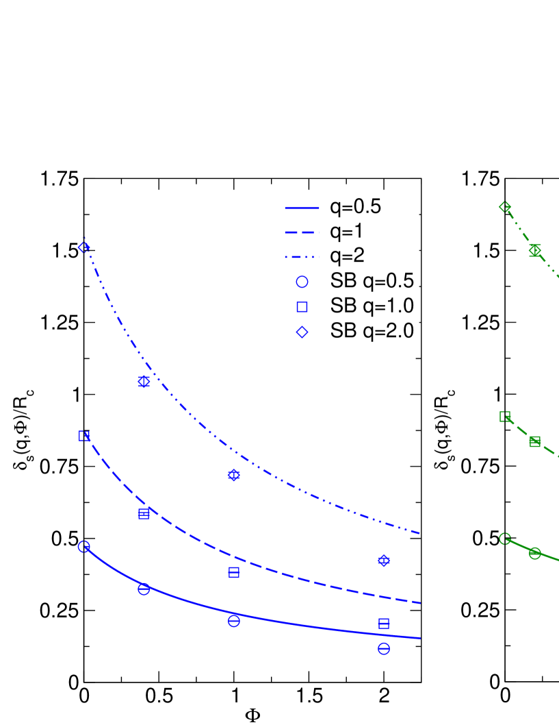
Figure 14: Depletion ratio $\delta_{s}(q,\Phi)/R_{c}$ for $z=\infty$ (left), $z=z^{(3)}$ (center), and $z=z^{(1)}$ (right). We report full-monomer (lines) and single-blob (SB, points) data as a function of $\Phi$.

Let us now compare finite-density results. In Fig. 12 we report the full-monomer and single-blob distribution function $g_{CM,cp}(r)$ for $q=0.5$. The curves vanish on the surface of the colloid ($b=0$) and then show some oscillations that become stronger as $\Phi$ increases. The coarse-grained model appears to reproduce well the full-monomer correlations for $z=z^{(1)}$, while deviations are observed already for $\Phi=1$ in the good-solvent case. Results for $q=2$ are reported in Fig. 13. In this case correlations are non zero even for $r\leq R_{c}$ ($d\leq 1/2$): since $q>1$, it is not unlikely that the polymer center of mass lies inside the colloid. Since the effective potential is soft, oscillations are tiny and, apparently, the coarse-grained model reasonably reproduces the full-monomer distribution function. However, at a closer look one notices some systematic deviations on the tails of the distributions, which are particularly relevant for the computation of $G_{cp}$, hence significantly affect the adsorption properties.

Finally, let us consider the depletion thickness. The single-blob results are compared with the full-monomer ones [we use interpolations (90)] in Fig. 14. In the good-solvent case, the single-blob model provides reasonably accurate estimates up to $\Phi\approx 2$ for $q=0.5$. As $q$ increases, the agreement worsens, as expected. For $q=2$, small deviations are already observed for $\Phi=0.4$. The single-blob model appears to be more accurate in the crossover region. For $z=z^{(1)}$ and $q=0.5$ good results are obtained up to $\Phi=4$, while for $q=2$, agreement is observed up to $\Phi\approx 1$.

VII Conclusions

In this paper we perform a detailed study of the solvation properties of a single colloid in a polymer solution. Beside the good-solvent case, which has already been extensively studied, see, e.g., Refs. deGennes-CR79 ; JLdG-79 ; EHD-96 ; HED-99 ; MEB-01 ; FS-01 ; LBMH-02-a ; FT-08 and references therein, we also consider the crossover between the good-solvent and the $\theta$ regime. We perform a detailed study for two intermediate cases. We consider $z=z^{(3)}$, which corresponds to $A_{2,pp}/A_{2,pp,GS}=\Psi/\Psi_{GS}=0.54$ (here $\Psi$ is the interpenetratio ratio often used in experimental work and $A_{2,pp,GS}$, $\Psi_{GS}$ are the good-solvent values), hence to solutions that have properties in between the good-solvent and the $\theta$ case. Moreover, we consider $z=z^{(1)}$, corresponding to $\Psi/\Psi_{GS}=0.18$, which corresponds to a solution close to the $\theta$ point.

We perform a detailed study of the depletion thickness in the dilute regime. For this purpose we relate solvation properties to polymer-colloid virial coefficients. We compute the second and the third virial coefficients in a large $q$ interval ($0\leq q\leq 50$ for the good-solvent case and $0\leq q\leq 30$ for $z=z^{(1)}$). The good-solvent results are compared with the existing field-theoretical predictions EHD-96 ; HED-99 ; MEB-01 , finding a reasonable agreement in all cases. We also consider the PRISM prediction FS-01 , which appears to be of limited quantitative interest, and the phenomenological prediction of Ref. FT-08 [see Eq. (63)], which turns out to describe the numerical data quite accurately for $0.2\mathrel{\hbox to0.0pt{\lower 3.0pt\hbox{$\mathchar 536\relax$}\hss}\raise 2.0pt\hbox{$\mathchar 316\relax$}}q\mathrel{\hbox to0.0pt{\lower 3.0pt\hbox{$\mathchar 536\relax$}\hss}\raise 2.0pt\hbox{$\mathchar 316\relax$}}4$.

We also perform a careful study at finite density for $q=0,0.5,1,2$. For all these values of $q$ and both in the good-solvent and in the crossover regime, we find that the ratio $\Delta(q,\Phi)=\delta_{s}(q,\Phi)/\delta_{s}(q,0)$ is approximately independent of $q$ for $\Phi\leq 4$, so that the $\Phi$ dependence and the $q$ dependence are approximately factorized. We do not have any theoretical explanation of this phenomenon, but we can easily argue that it can only hold for $q$ and $\Phi$ not too large. First, we can compute exactly the ratio $\Delta(q,\Phi)$ for $q\to\infty$. Then, we find that the limiting $\Delta(\infty,\Phi)$ differs significantly from what we obtain for $q\leq 2$, indicating that, as $q$ increases, $\Delta(q,\Phi)$ should gradually change from its value for $q\leq 2$ to the infinite-$q$ limiting curve, hence it should be $q$-dependent. Second, a general argument predicts that $\delta(q,\Phi)$ becomes independent of $q$ for $\Phi\to\infty$. Hence, deep in the semidilute regime $\Delta(q,\Phi)$ should have the same $q$-dependence as $1/\delta(q,0)$, which is quite significant. We compare the numerical good-solvent results with field-theory predictions MEB-01 . We find that the large-$\Phi$ prediction of Ref. MEB-01 describes well the numerical data, confirming the accuracy of the field-theory approach.

We also analyze depletion properties of the single-blob coarse-grained model. As expected, they are accurate as long as polymer-polymer overlaps are rare and colloids are large compared with the polymers, i.e. for $q\mathrel{\hbox to0.0pt{\lower 3.0pt\hbox{$\mathchar 536\relax$}\hss}\raise 2.0pt\hbox{$\mathchar 316\relax$}}1$. As already observed in Ref. DPP-thermal , we find that the accuracy of the coarse-grained model increases as $z$ decreases. While in the good-solvent case some deviations are observed for $\Phi\mathrel{\hbox to0.0pt{\lower 3.0pt\hbox{$\mathchar 536\relax$}\hss}\raise 2.0pt\hbox{$\mathchar 318\relax$}}1$, even for large colloids ($q=0.5$), for $z=z^{(1)}$ reasonably good results are obtained up to $\Phi\approx 4$, well inside the semidilute regime.

Appendix A Virial expansion for multicomponent systems

In this Appendix we wish to study the virial expansion for a multicomponent system of flexible molecules, computing explicitly the flexibility contribution due to the polyatomic nature of the molecules. We extend here the results presented in Refs. CMP-06 ; CMP-08-star .

We start by considering a multicomponent system in the grand canonical ensemble. The grand partition function is given by

$$\Xi=\sum_{N_{1},\ldots,N_{k}}{z_{1}^{N_{1}}\over N_{1}!}\ldots{z_{k}^{N_{k}}\over N_{k}!}Q(N_{1},\ldots,N_{k}),$$ (92)

where $k$ is the number of species present, $z_{1}$, $\ldots$, $z_{k}$ are the corresponding fugacities, $Q(N_{1},\ldots,N_{k})$ is the canonical partition function of the system. If $V$ is the volume of the box, we define reduced fugacities as

$$\hat{z}_{1}=z_{1}Q(1,0\ldots,0)/V,\qquad\ldots$$

$$\hat{z}_{k}=z_{k}Q(0,\ldots,0,1)/V.$$ (93)

Then, at third order in the fugacities we obtain the expansion

$$\beta P = {1\over V}\ln\Xi=\sum_{\alpha}\hat{z}_{\alpha}+{1\over 2}\sum_{\alpha\beta}\hat{z}_{\alpha}\hat{z}_{\beta}I_{2}(\alpha,\beta)+$$ (94)

$${1\over 6}\sum_{\alpha\beta\gamma}\hat{z}_{\alpha}\hat{z}_{\beta}\hat{z}_{\gamma}\left[I_{3}(\alpha\beta\gamma)+I_{2}(\alpha\beta)I_{2}(\alpha\gamma)+\right.$$

$$\qquad I_{2}(\alpha\beta)I_{2}(\beta\gamma)+I_{2}(\alpha\gamma)I_{2}(\beta\gamma)+$$

$$\qquad\left.T_{2}(\alpha,\beta\gamma)+T_{2}(\beta,\alpha\gamma)+T_{2}(\gamma,\alpha\beta)\right].$$

To define the integrals $I_{2}(\alpha\beta)$, $I_{3}(\alpha\beta\gamma)$ and $T_{2}(\alpha,\beta\gamma)$, we should associate to each molecule a specific point $X$. The choice of $X$ is irrelevant, as long as $X$ is a weighted average of the positions of the atoms belonging to the molecule. For instance one can take the center of mass of the molecule, but for a linear polymer an equally good choice corresponds to choosing the first or the central monomer. Then, we define the average $\langle\cdot\rangle_{\alpha,{\bf r};\beta,{\bf s}}$ as the average over all pairs of isolated molecules of type $\alpha$ and $\beta$, respectively, such that point $X$ of molecule $\alpha$ is fixed in ${\bf r}$ and point $X$ of molecule $\beta$ is fixed in ${\bf s}$. Analogously, we define the average $\langle\cdot\rangle_{\alpha,{\bf r};\beta,{\bf s};\gamma,{\bf t}}$ over all triples of isolated molecules. Then, the integral $I_{2}(\alpha\beta)$ is defined as

$$I_{2}(\alpha\beta)=\int d{\bf r}\langle e^{-\beta U_{{\rm inter},\alpha\beta}}-1\rangle_{\alpha,{\bf 0};\beta,{\bf r}}$$ (95)

where $U_{{\rm inter},\alpha\beta}$ is the intermolecular energy between an $\alpha$ and a $\beta$ molecule. Analogously we define

$$I_{3}(\alpha\beta\gamma)=\int d{\bf r}d{\bf s}\langle(e^{-\beta U_{\rm inter,\alpha\beta}}-1)$$

$$\qquad\times(e^{-\beta U_{\rm inter,\alpha\gamma}}-1)(e^{-\beta U_{\rm inter,\beta\gamma}}-1)\rangle_{\alpha,{\bf 0};\beta,{\bf r};\gamma,{\bf s}},$$ (96)

$$T_{2}(\alpha,\beta\gamma)=\int d{\bf r}d{\bf s}\langle(e^{-\beta U_{\rm inter,\alpha\beta}}-1)$$

$$\qquad\times(e^{-\beta U_{\rm inter,\alpha\gamma}}-1)\rangle_{\alpha,{\bf 0};\beta,{\bf r};\gamma,{\bf s}}-I_{2}(\alpha\beta)I_{2}(\alpha\gamma).$$ (97)

The integral $T_{2}$ represents the flexibility contribution: if the $\alpha$ molecule is rigid, then $T_{2}(\alpha,\beta\gamma)=0$. It is easy to generalize the bounds for $T_{2}(\alpha,\alpha\alpha)$ found in Ref. CMP-08-star obtaining

$$T_{2}(\alpha,\beta\beta)\geq 0,$$ (98)

$$|T_{2}(\alpha,\beta\gamma)|\leq{1\over 2}\left[T_{2}(\alpha,\beta\beta)+T_{2}(\alpha,\gamma\gamma)\right].$$ (99)

We wish now to express the pressure in terms of the concentrations $\rho_{\alpha}$:

$$\rho_{\alpha}={\langle N_{\alpha}\rangle\over V}=\hat{z}_{\alpha}{\partial\beta P\over\partial\hat{z}_{\alpha}}.$$ (100)

Expressing the fugacities in terms of the concentrations, we obtain

$$\hat{z}_{\alpha} = \rho_{\alpha}-\rho_{\alpha}\sum_{\beta}I_{2}(\alpha\beta)\rho_{\beta}$$

$$+{1\over 2}\rho_{\alpha}\sum_{\beta\gamma}\rho_{\beta}\rho_{\gamma}\left[I_{2}(\alpha\beta)I_{2}(\alpha\gamma)-I_{3}(\alpha\beta\gamma)\right.$$

$$\left.-T_{2}(\alpha,\beta\gamma)-T_{2}(\beta,\alpha\gamma)-T_{2}(\gamma,\alpha\beta)\right].$$

Substituting this expression in Eq. (94), we obtain finally

$$\beta P = \sum_{\alpha}\rho_{\alpha}-{1\over 2}\sum_{\alpha\beta}\rho_{\alpha}\rho_{\beta}I_{2}(\alpha\beta)$$ (102)

$$-{1\over 3}\sum_{\alpha\beta\gamma}\rho_{\alpha}\rho_{\beta}\rho_{\gamma}\left[I_{3}(\alpha\beta\gamma)\right.$$

$$\qquad\left.+T_{2}(\alpha,\beta\gamma)+T_{2}(\beta,\alpha\gamma)+T_{2}(\gamma,\alpha\beta)\right].$$

We can now specialize this expression to a polymer-colloid mixture. If the suffixes ”c” and ”p” refer to the colloids and polymers, respectively, we can expand the pressure as in Eq. (31), neglecting terms that are of fourth order in the concentrations. The virial coefficients are then given by

$$B_{2,c} = -{1\over 2}I_{2}(cc),$$ (103)

$$B_{2,p} = -{1\over 2}I_{2}(pp),$$ (104)

$$B_{2,cp} = -I_{2}(cp),$$ (105)

$$B_{3,c} = -{1\over 3}I_{3}(ccc),$$ (106)

$$B_{3,p} = -{1\over 3}I_{3}(ppp)-T_{2}(p,pp),$$ (107)

$$B_{3,ccp} = -I_{3}(ccp)-T_{2}(p,cc),$$ (108)

$$B_{3,cpp} = -I_{3}(cpp)-2T_{2}(p,cp),$$ (109)

where we used the fact that the colloid is rigid, hence $T_{2}(c,\alpha\beta)=0$ for any $\alpha$ and $\beta$.

For our lattice model, integrals over the polymer positions are replaced by lattice sums, which are evaluated by using the hit-or-miss procedure applied in Refs. LMS-95 ; CMP-06 to the computation of the polymer virial coefficients. The flexibility contributions are usually quite small CMP-06 ; CMP-08-star ; Kofke-11-12 . For the mixed third virial coefficients, their relevance depends on $q$. The flexibility correction to $B_{3,ccp}$ and $B_{3,cpp}$ decreases as $q\to 0$. The ratio $T_{2}(p,cc)/B_{3,ccp}$ is equal to 8%, 3%, 1% for $q=3,1,0.4$, respectively, in the good-solvent case. The analogous ratio $2T_{2}(p,cp)/B_{3,cpp}$ is slightly larger. It is equal to 9%, 5%, 2% for $q=3,1,0.4$, respectively.

The ratio $T_{2}/B_{3}$ gives us a hint on the role of the neglected three-body forces in single-blob coarse-grained models. Indeed, if the flexibility integral can be neglected, we can infer that the following factorization holds approximately:

$$\langle(e^{-\beta U_{\rm inter,\alpha\beta}}-1)(e^{-\beta U_{\rm inter,\alpha\gamma}}-1)\rangle_{\alpha,{\bf 0};\beta,{\bf r};\gamma,{\bf s}}$$ (110)

$$=\langle(e^{-\beta U_{\rm inter,\alpha\beta}}-1)\rangle_{\alpha,{\bf 0};\beta,{\bf r}}\langle(e^{-\beta U_{\rm inter,\alpha\gamma}}-1)\rangle_{\alpha,{\bf 0};\gamma,{\bf s}}.$$

By definition we have

$$\langle(e^{-\beta U_{\rm inter,\alpha\beta}}-1)\rangle_{\alpha,{\bf 0};\beta,{\bf r}}=e^{-\beta V_{SB,\alpha\beta}({\bf r})},$$ (111)

where $V_{SB,\alpha\beta}({\bf r})$ is the pair potential in the single-blob model. Therefore, the previous factorization condition implies

$$I_{3}(\alpha\beta\gamma) \approx \int d{\bf r}d{\bf s}\,\left(e^{-\beta V_{SB,\alpha\beta}({\bf r})}-1\right)$$

$$\times\left(e^{-\beta V_{SB,\alpha\gamma}({\bf s})}-1\right)\left(e^{-\beta V_{SB,\beta\gamma}({\bf r}-{\bf s})}-1\right).$$

The right-hand side is the integral in the coarse-grained model. Hence, if $T_{2}$ is negligible, the third virial coefficient in the model is approximately equal to that in the coarse-grained model, indicating that the effective three-body forces are small (see the appendix of Ref. DPP-12-softspheres for the explicit expression of the third virial coefficient in terms of three-body forces).

Appendix B Asymptotic behavior of the virial coefficients for $q\to 0$

To compute the limiting expression of the virial coefficients for $q\to 0$, let us first define $U_{\rm int,cp}(r)$ as the intermolecular energy between a colloid in the origin and a polymer such that its first monomer is in ${\bf r}$. The choice of the first monomer is arbitrary and the same result would have been obtained by taking any other monomer. Then, let

$$f_{cp}(r)=e^{-\beta U_{\rm int,cp}(r)}-1$$ (113)

be the corresponding Mayer function, which satisfies $f_{cp}(r)=1$ for $r<R_{c}$. Analogously we define the polymer-polymer Mayer function $f_{pp}(r)$, where $r$ is the distance between the first monomers of the two polymers. Using the fact that $f_{cp}(r)=-1$ for $r\leq R_{c}$ and defining $z=r-R_{c}$, we obtain

$$B_{2,cp} = {4\pi R_{c}^{3}\over 3}-4\pi\int_{R_{c}}^{\infty}drr^{2}\langle f_{cp}(r)\rangle$$

$$\approx {4\pi R_{c}^{3}\over 3}-4\pi R^{2}_{c}\int_{0}^{\infty}dz\,\langle\hat{f}_{cp}(z)\rangle$$

$$= {4\pi R_{c}^{3}\over 3}+4\pi R^{2}_{c}P_{1,p},$$

where $\hat{f}_{cp}(z)=f_{cp}(R_{c}+z)$ and

$$P_{1,p}=-\int_{0}^{\infty}dz\,\langle\hat{f}_{cp}(z)\rangle.$$ (115)

The integral $P_{1,p}$ corresponds to a polymer interacting with an impenetrable plane. In our model, in which we have a hard-interaction between monomers and hard wall, we can further simplify $P_{1,p}$. If $z_{\rm min}$ is the smallest value of the $z$ coordinate of the first point of the walk such that the walk does not intersect the wall, we have $P_{1,p}=\langle z_{\rm min}\rangle$. This expression can be rewritten in a form which is independent of the coordinates of the first monomer. Indeed, define

$$z_{m}=\min_{k}z_{k},\qquad z_{M}=\max_{k}z_{k},$$ (116)

where $z_{k}$ is the $z$ coordinate of the $k$-th monomer. Then, we can rewrite $z_{\rm min}=z_{1}-z_{m}$. If we now consider the walk which is obtained by means of a specular reflection with respect to the plane $z=z_{1}$ we obtain $z_{\rm min}=z_{M}-z_{1}$. Hence, if we average the two contributions we obtain

$$P_{1,p}={1\over 2}\langle z_{M}-z_{m}\rangle,$$ (117)

in which there is no reference to the first monomer, which was arbitrarily chosen to define the integrations.

Let us now consider the third virial coefficient $B_{3,cpp}$. We have

$$B_{3,cpp} = -\int d{\bf r}\,d{\bf s}\,\left\{\langle f_{cp}(r)f_{cp}(s)f_{pp}(\rho)\rangle+\right.$$ (118)

$$\left.\langle f_{cp}(r)f_{pp}(\rho)\rangle+\langle f_{cp}(s)f_{pp}(\rho)\rangle\right.$$

$$\left.-\langle f_{cp}(r)\rangle\langle f_{pp}(\rho)\rangle-\langle f_{cp}(s)\rangle\langle f_{pp}(\rho)\rangle\right\},$$

where $\rho=|{\bf s}-{\bf r}|$. We can further simplify this expression defining

$$A(r,s)=e^{-\beta U_{{\rm inter},cp}(r)-\beta U_{{\rm inter},cp}(s)}-1,$$ (119)

and the function $I(r)$ such that $I(r)=1$ for $r\leq R_{c}$ and $I(r)=0$ otherwise. Since $A(r,s)=-1$ and $f_{cp}(r)=-1$ for $r<R_{c}$, we can write

$$\int d{\bf r}\,d{\bf s}\,\left\{\langle f_{cp}(r)f_{cp}(s)f_{pp}(\rho)\rangle\right.+$$

$$\qquad\left.\langle f_{cp}(r)f_{pp}(\rho)\rangle+\langle f_{cp}(s)f_{pp}(\rho)\rangle\right\}$$

$$=\int d{\bf r}\,d{\bf s}\,\langle A(r,s)f_{pp}(\rho)\rangle$$

$$=\int d{\bf r}\,d{\bf s}\,\left\{-\langle f_{pp}(\rho)\rangle I(r)\right.$$

$$\qquad\left.+\langle A(r,s)f_{pp}(\rho)\rangle[1-I(r)]\right\}$$

$$=\int d{\bf r}\,d{\bf s}\,\left\{\langle f_{cp}(r)\rangle\langle f_{pp}(\rho)\rangle I(r)\right.$$

$$\qquad+\left.\langle A(r,s)f_{pp}(\rho)\rangle[1-I(r)]\right\}$$

$$=\int d{\bf r}\,d{\bf s}\,\left\{\langle f_{cp}(r)\rangle\langle f_{pp}(\rho)\rangle\right.$$ (120)

$$\qquad\left.+\left[\langle A(r,s)f_{pp}(\rho)\rangle-\langle f_{cp}(r)\rangle\langle f_{pp}(\rho)\rangle\right][1-I(r)]\right\}.$$

Therefore, we can rewrite

$$B_{3,cpp}=-\int d{\bf r}\,d{\bf s}\,\left\{\vphantom{\hat{R}}\left[\langle A(r,s)f_{pp}(\rho)\rangle\right.\right.$$ (121)

$$\qquad\left.\left.-\vphantom{\hat{R}}\langle f_{cp}(r)\rangle\langle f_{pp}(\rho)\rangle\right][1-I(r)]-\langle f_{cp}(r)\rangle\langle f_{pp}(\rho)\rangle\right\}.$$

To rewrite this term in a more transparent way, let us consider $B_{2,cp}B_{2,pp}$ which we rewrite as

$$2B_{2,cp}B_{2,pp} = \int d{\bf r}\,d{\bf s}\,\langle f_{cp}(r)\rangle\langle f_{pp}(\rho)\rangle.$$ (122)

Using this expression we obtain finally

$$B_{3,cpp}=2B_{2,cp}B_{2,pp}$$ (123)

$$-\int d{\bf r}\,d{\bf s}\,[1-I(r)]\left\{\langle A(r,s)f_{pp}(\rho)\rangle-\langle f_{cp}(r)\rangle\langle f_{pp}(\rho)\rangle\right\}$$

The remaining integral is a surface contribution. Indeed, for $r\geq R_{c}$ the function $A(r,s)$ is different from zero only if $r-R_{c}$ is of order of a few times $\hat{R}_{g}$. Moreover, since the range of $f_{pp}(\rho)$ is also of order $\hat{R}_{g}$, the integral gets contributions only if $|{\bf r}-{\bf s}|$ is of order $\hat{R}_{g}$. Hence, a nonvanishing contribution is obtained only if $|R-s|$ is of the order of a few times $\hat{R}_{g}$. To make this explicit, let us introduce bipolar coordinates so that

$$B_{3,cpp}=2B_{2,cp}B_{2,pp}$$

$$\qquad-8\pi^{2}\int_{R_{c}}^{\infty}rdr\,\int_{0}^{\infty}sds\int_{|r-s|}^{r+s}\rho d\rho$$

$$\qquad\left\{\langle A(r,s)f_{pp}(\rho)\rangle-\langle f_{cp}(r)\rangle\langle f_{pp}(\rho)\rangle\right\}$$ (124)

We now change variable, defining

$$z_{1}=r-R_{c},\quad z_{2}=s-R_{c}\quad x=\sqrt{\rho^{2}-(z_{1}-z_{2})^{2}}.$$ (125)

Taking the limit $R_{c}\to\infty$, we obtain

$$B_{3,cpp}=2B_{2,cp}B_{2,pp}$$ (126)

$$\qquad-4\pi R_{c}^{2}\int_{0}^{\infty}(2\pi x)dx\int_{0}^{\infty}dz_{1}\int_{-\infty}^{\infty}dz_{2}$$

$$\qquad\left\{\langle A(R_{c}+z_{1},R_{c}+z_{2})f_{pp}(\rho)\rangle-\langle\hat{f}_{cp}(z_{1})\rangle\langle f_{pp}(\rho)\rangle\right\}.$$

We define $\hat{A}(z_{1},z_{2})={A}(R_{c}+z_{1},R_{c}+z_{2})$, which takes the value $-1$ whenever $z_{1}$ or $z_{2}$ is negative, and

$$P_{2,pp}=2P_{1,p}B_{2,pp}$$ (127)

$$\qquad-\int_{0}^{\infty}(2\pi x)dx\int_{0}^{\infty}dz_{1}\int_{-\infty}^{\infty}dz_{2}\langle\hat{A}(z_{1},z_{2})f_{pp}(\rho)\rangle.$$

This allows us to write

$$B_{3,cpp}=2B_{2,cp}B_{2,pp}+4\pi R_{c}^{2}P_{2,pp}.$$ (128)

Using this expression we can compute the expansion of $\delta_{s}$ for $q\to 0$. We obtain

$$\delta_{s}=P_{1,p}+\rho_{p}P_{2,pp}+O(\rho_{p}^{2}),$$ (129)

which coincides with that valid for polymers in the presence of an impenetrable plane. From Eq. (128) and (B) we obtain finally Eq. (70).

For our lattice model the integral $\hat{P}_{2,pp}=P_{2,pp}-2P_{1,p}B_{2,pp}$ can be given a simpler form, averaging again over the walks that are obtained by specular reflections with respect to the planes that go through the first monomer and are parallel the surface. Let $\omega_{1}$ and $\omega_{2}$ be two lattice chains and $z_{k}^{(1)}$ and $z_{k}^{(2)}$ be the $z$-coordinates of their $k$-th monomers. Then, define $T(\omega_{2},{\bf r})$ as the lattice walk that is obtained by translating $\omega_{2}$ by the lattice vector ${\bf r}$ and the function $H(\omega,\overline{z})$ which takes the value $+1$ if the walk $\omega$ intersects the plane $z=\overline{z}$ and the value $0$ otherwise. If $z_{m}^{(i)}=\min z_{k}^{(i)}$, $z_{M}^{(i)}=\max z_{k}^{(i)}$, $Z_{m}=z_{m}^{(1)}+z_{m}^{(2)}-z_{M}^{(2)}$, and $Z_{M}=z_{M}^{(1)}+z_{M}^{(2)}-z_{m}^{(2)}$ we have

$$\hat{P}_{2,pp}=-{1\over 2}\left\langle\sum_{z_{1}=Z_{m}}^{Z_{M}}\sum_{{\bf r}}\left\{H[\omega_{1},z_{1}]+H[T(\omega_{2},{\bf r}),z_{1}]\right.\right.$$

$$\qquad\left.\left.-H[\omega_{1},z_{1}]H[T(\omega_{2},{\bf r}),z_{1}]\right\}\left(1-e^{-wN_{\rm int}}\right)\right\rangle,$$ (130)

where the sum over ${\bf r}$ is over all lattice translations and $N_{\rm int}$ is the number of intersections between $\omega_{1}$ and the translated $T(\omega_{2},{\bf r})$. The sums are evaluated by using the obvious generalization of the hit-or-miss procedure applied in Refs. LMS-95 ; CMP-06 to the computation of the polymer virial coefficients.

Finally, we shall discuss the third-virial coefficient $B_{3,ccp}$. Since this quantity is not relevant for the depletion we will only compute the leading term, which can be obtained by approximating the polymer with a hard sphere of zero radius. Thus, we obtain for $q\to 0$

$$B_{3,ccp}\hat{R}_{g}^{-6}={16\pi^{2}\over 9q^{6}}.$$ (131)

Appendix C Supplementary material

C.1 Low-density virial coefficients and depletion thickness

In this supplementary material we report the numerical estimates of the virial coefficients and of the depletion thickness in the low-density limit. In the good-solvent case, for $q\leq 3$ we have results for $L=240$, 600, and 2400: in this case, the universal large-$L$ limit has been obtained by performing an extrapolation of the results with $a+b/L^{\nu}+c/L$. For $q\geq 4$, we have results for $L=6000$ and 24000, which have been extrapolated to $a+b/L^{\nu}$. Here $\nu$ is the usual Flory exponent, $\nu=0.587597$. In the crossover region, for $q\leq 3$ we have results for $L=120$, 240, 600, 1200, and 2400: they have been fitted to $a+b/\sqrt{L}+c/L$. For $q\geq 4$ we only have results for $L=6000$ and 30000: they have been extrapolated using $a+b/\sqrt{L}$. The results of the extrapolations are reported in Tables 8, 9, and 10. In Table 11 we report single-blob results. Of course, here no extrapolation is needed.

Table 8: Estimates of the asymptotic, universal adimensional virial combinations $A_{2,cp}=B_{2,cp}\hat{R}_{g}^{-3}$, $A_{3,cpp}=B_{3,cpp}\hat{R}_{g}^{-6}$, $A_{3,ccp}=B_{3,ccp}\hat{R}_{g}^{-6}$, for $z=\infty$ (good-solvent case) and for $z=z^{(1)}$.

	$z=\infty$			$z=z^{(1)}$
$q$	$A_{2,cp}$	$A_{3,cpp}$	$A_{3,ccp}$	$A_{2,cp}$	$A_{3,cpp}$	$A_{3,ccp}$
50	0.1097(2)	0.015(5)
40	0.1467(4)	0.023(6)
35	0.1744(4)	0.029(7)
30	0.2131(5)	0.0442(9)		0.416(1)	0.032(2)
25	0.2702(7)	0.062(10)		0.504(1)	0.047(2)
20	0.3615(9)	0.108(15)		0.639(1)	0.073(3)
15	0.527(1)	0.20(2)		0.870(1)	0.128(5)
10	0.899(2)	0.57(3)	0.018(2)	1.360(2)	0.272(6)	0.014(1)
8	1.210(3)	0.97(4)	0.040(3)	1.750(3)	0.42(1)	0.044(8)
6	1.782(4)	1.90(6)	0.144(6)	2.446(4)	0.76(1)	0.156(6)
4	3.114(7)	5.0(1)	0.82(1)	4.010(6)	1.67(2)	0.95(2)
3	4.71(1)	10.2(1)	2.82(3)	5.807(8)	2.96(2)	3.35(2)
2	8.65(2)	26.1(2)	16.8(1)	10.20(1)	6.73(4)	19.55(8)
1.75	10.67(2)	35.7(3)	30.1(2)	12.41(2)	8.87(5)	35.0(1)
1.5	13.69(3)	51.2(4)	59.4(3)	15.71(2)	12.29(7)	68.7(2)
1.25	18.60(4)	78.6(1)	132.9(7)	21.02(3)	18.1(1)	152.7(5)
1.0	27.54(6)	133.3(9)	360(2)	30.61(5)	29.5(1)	409(1)
0.8	41.7(1)	228.5(15)	984(5)	45.62(7)	48.7(2)	1107(4)
0.6	73.45(20)	462(3)	3680(20)	79.1(1)	94.9(5)	4080(15)
0.5	107.4(3)	726(5)	8630(45)	114.5(2)	146.4(7)	9500(30)
0.4	174.5(4)	1281(8)	24900(150)	184.4(3)	253(1)	27100(90)
0.3	337.7(9)	2700(20)	101000(550)	352.9(6)	525(2)	108700(400)
0.2	909(2)	8000(50)	783000(4000)	937(2)	1520(7)	827000(3000)

Table 9: Estimates of the asymptotic, universal adimensional virial combinations $A_{2,cp}=B_{2,cp}\hat{R}_{g}^{-3}$, $A_{3,cpp}=B_{3,cpp}\hat{R}_{g}^{-6}$, $A_{3,ccp}=B_{3,ccp}\hat{R}_{g}^{-6}$, for $z=z^{(3)}$.

$q$	$A_{2,cp}$	$A_{3,cpp}$	$A_{3,ccp}$
3	5.53(2)	7.7(1)	3.31(2)
2	9.81(1)	18.2(1)	19.19(7)
1.75	11.97(2)	24.1(1)	34.3(1)
1.5	15.20(1)	33.7(1)	67.1(2)
1.25	20.42(3)	50.1(2)	149.0(5)
1.0	29.85(4)	82.6(3)	399(1)
0.8	44.63(6)	138.1(5)	1082(3)
0.6	77.7(1)	272(1)	4000(15)
0.5	112.8(2)	423.2(15)	9300(30)
0.4	182.0(3)	737(3)	26625(85)
0.3	350(5)	1533(6)	107100(300)
0.2	932(2)	4470(20)	818000(3000)

Table 10: Depletion thickness $\delta_{s,0}/R_{c}=\delta_{s}(\Phi=0)/R_{c}$ at zero density and first density correction $\delta_{1}(q)$.

	$z=\infty$		$z=z^{(3)}$		$z=z^{(1)}$
$q$	$\delta_{s,0}/R_{c}$	$\delta_{1}$	$\delta_{s,0}/R_{c}$	$\delta_{1}$	$\delta_{s,0}/R_{c}$	$\delta_{1}$
50	13.85(9)	$-$0.927(4)
40	12.09(1)	$-$0.934(4)
35	11.13(1)	$-$0.939(4)
30	10.117(9)	$-$0.944(4)			12.897(7)	$-$0.1637(5)
25	9.027(8)	$-$0.952(4)			11.345(6)	$-$0.1638(5)
20	7.838(7)	$-$0.960(4)			9.685(6)	$-$0.1643(8)
15	6.515(6)	$-$0.975(4)			7.883(5)	$-$0.1655(6)
10	4.987(5)	$-$0.991(4)			5.872(4)	$-$0.1665(7)
8	4.289(4)	$-$1.001(3)			4.980(3)	$-$0.1672(8)
6	3.512(3)	$-$1.016(4)			4.015(3)	$-$0.1675(6)
4	2.624(3)	$-$1.032(4)			2.942(2)	$-$0.1678(8)
3	2.119(2)	$-$1.035(3)	2.292(1)	$-$0.519(2)	2.343(6)	$-$0.168(1)
2	1.547(2)	$-$1.046(4)	1.656(1)	$-$0.520(2)	1.6893(5)	$-$0.168(1)
1.75	1.390(2)	$-$1.047(5)	1.484(1)	$-$0.521(1)	1.5132(5)	$-$0.168(1)
1.5	1.226(2)	$-$1.049(5)	1.306(1)	$-$0.522(2)	1.3304(4)	$-$0.168(1)
1.25	1.054(2)	$-$1.050(6)	1.1194(9)	$-$0.523(2)	1.1401(4)	$-$0.168(1)
1.0	0.873(41)	$-$1.052(7)	0.9243(8)	$-$0.523(3)	0.9408(4)	$-$0.1675(15)
0.8	0.720(1)	$-$1.048(9)	0.7605(8)	$-$0.522(4)	0.7737(4)	$-$0.167(2)
0.6	0.559(1)	$-$1.05(1)	0.5884(7)	$-$0.521(4)	0.5982(3)	$-$0.167(2)
0.5	0.474(1)	$-$1.05(1)	0.4988(7)	$-$0.520(4)	0.5069(3)	$-$0.167(2)
0.4	0.387(1)	$-$1.04(2)	0.4063(7)	$-$0.516(6)	0.4128(3)	$-$0.167(3)
0.3	0.296(1)	$-$1.05(2)	0.3107(7)	$-$0.515(8)	0.3155(3)	$-$0.166(3)
0.2	0.202(1)	$-$1.04(3)	0.2116(6)	$-$0.51(1)	0.2146(3)	$-$0.166(5)

Table 11: Virial coefficients, depletion thickness $\delta_{s,0}/R_{c}=\delta_{s}(\Phi=0)/R_{c}$ at zero density and first density correction $\delta_{1}(q)$ in the single-blob model.

$z$	$q$	$A_{2,cp}$	$\delta_{s,0}/R_{c}$	$\delta_{1}$	$A_{3,cpp}$	$A_{3,ccp}$
$z^{(1)}$	0.5	114.376(5)	0.50563(2)	$-$0.1775(1)	141.32(7)	9518(2)
	1.0	30.555(3)	0.9394(5)	$-$0.1838(1)	26.64(2)	399.0(3)
	2.0	10.155(1)	1.68675(9)	$-$ 0.18620(7)	5.299(6)	16.94(3)
$z^{(3)}$	0.5	112.496(5)	0.49734(2)	$-$0.5491(3)	409.2(2)	9285(2)
	1.0	29.750(2)	0.92221(5)	$-$0.5656(3)	74.94(6)	385.2(2)
	2.0	9.762(1)	1.6516(9)	$-$ 0.5707(2)	14.27(1)	16.01(3)
$\infty$	0.5	106.787(6)	0.47156(3)	$-$1.0967(9)	701.2(4)	8565(2)
	1.0	26.796(2)	0.85635(4)	$-$1.1443(4)	116.55(6)	331.8(2)
	2.0	8.2866(9)	1.51068(9)	$-$1.1468(3)	19.16(2)	12.55(2)

C.2 Scaling corrections in the presence of colloid-polymer interactions

In the field-theoretical approach to critical phenomena, the presence of an impenetrable boundary gives rise to additional irrelevant surface operators, which, in turn, give rise to new corrections to scaling. For the case of a nonadsorbing boundary, the question was analyzed by H. W. Diehl, S. Dietrich, and E. Eisenriegler [Phys. Rev. B 27, 2937 (1983)]. They found that the leading surface correction is associated with an exponent $\omega=-\nu$. We have performed a careful check of this prediction, by considering the universal combinations $R_{1,p}$. Estimates for several values of $L$ are reported in Table 12 (good-solvent case) and in Table 14 ($z=z^{(1)}$). The results have been fitted to $R_{1,p}^{*}+a/L^{\theta}$, where $R_{1,p}^{*},a$, and $\theta$ are taken as free parameters. The results of the fits of the good-solvent data are reported in Table 13. They are clearly consistent with $\theta=\nu\approx 0.588$. For $z=z^{(1)}$, the results reported in Table 15 are consistent with $\theta=1/2$, as expected.

Table 12: Estimates of the combinations $R_{1,p}$ and $R_{2,pp}$ for $z=\infty$ (good-solvent case), as a function of the length $L$ of the chains.

$L$	$R_{1,p}$	$R_{2,pp}$
120	0.98351(3)	$-$5.354(3)
240	1.00905(7)	$-$5.184(10)
480	1.02597(3)	$-$4.928(4)
600	1.03019(4)	$-$4.890(5)
900	1.03650(2)	$-$4.789(3)
1200	1.04018(3)	$-$4.752(3)
1800	1.04446(4)	$-$4.704(4)
2400	1.04683(11)	$-$4.683(12)
3600	1.04978(3)	$-$4.633(3)
4800	1.05142(4)	$-$4.614(3)
6000	1.05255(5)	$-$4.602(6)
9000	1.05418(8)	$-$4.576(8)
12000	1.05514(9)	$-$4.566(9)
24000	1.05696(8)	$-$4.541(8)

Table 13: Fits of $R_{1,p}$ to $R_{1,p}^{*}+a/L^{\theta}$, including only data satisfying $L\geq L_{\rm min}$. $\chi^{2}$ is the sum of the residuals and DOF is the number of degrees of freedom of the fit. Results for the good-solvent ($z=\infty$) case.

$L_{\rm min}$	$\chi^{2}$/DOF	$R_{1,p}^{*}$	$\theta$
120	4.75/11	1.06057(5)	0.578(1)
240	3.32/10	1.06063(7)	0.575(2)
480	2.32/9	1.06057(9)	0.578(3)
600	2.17/8	1.06060(12)	0.576(5)
900	1.26/7	1.06052(15)	0.581(6)
1200	1.23/6	1.06050(18)	0.582(9)
1800	1.19/5	1.06053(23)	0.580(14)

Table 14: Estimates of the combinations $R_{1,p}$ and $R_{2,pp}$ for $z=z^{(1)}$, as a function of the chain length $L$.

$L$	$R_{1,p}$	$R_{2,pp}$
120	1.01296(10)	$-$1.093(3)
240	1.04504(9)	$-$0.997(2)
600	1.07343(11)	$-$0.910(2)
1200	1.08795(12)	$-$0.873(3)
2400	1.09810(9)	$-$0.839(2)
6000	1.10701(9)	$-$0.812(2)
12000	1.11140(19)	$-$0.797(4)
30000	1.11539(19)	$-$0.787(4)

Table 15: Fits of $R_{1,p}$ to $R_{1,p}^{*}+a/L^{\theta}$, including only data satisfying $L\geq L_{\rm min}$. $\chi^{2}$ is the sum of the residuals and DOF is the number of degrees of freedom of the fit. Results for $z=z^{(1)}$.

$L_{\rm min}$	$\chi^{2}$/DOF	$R_{1,p}^{*}$	$\theta$
120	3.35/5	1.1224(2)	0.501(2)
240	2.80/4	1.1223(2)	0.503(3)
600	0.14/3	1.1218(4)	0.514(7)
1200	0.11/2	1.1219(5)	0.512(14)

References

- (1) W. C. K. Poon, J. Phys.: Condensed Matter 14, R859 (2002).
- (2) M. Fuchs and K. S. Schweizer, J. Phys.: Condensed Matter 14, R239 (2002).
- (3) R. Tuinier, J. Rieger, and C. G. de Kruif, Adv. Coll. Interface Sci. 103, 1 (2003).
- (4) K. J. Mutch, J. S. van Duijneveldt, and J. Eastoe, Soft Matter 3, 155 (2007).
- (5) G. J. Fleer and R. Tuinier, Adv. Coll. Interface Sci. 143, 1 (2008).
- (6) O. Myakonkaya and J. Eastoe, Adv. Coll. Interface Sci. 149, 39 (2009).
- (7) A. A. Louis, P. G. Bolhuis, E. J. Meijer, and J. P. Hansen, J. Chem. Phys. 116, 10547 (2002).
- (8) A. A. Louis, P. G. Bolhuis, E. J. Meijer, and J. P. Hansen, J. Chem. Phys. 117, 1893 (2002).
- (9) E. Eisenriegler, A. Hanke and S. Dietrich, Phys. Rev. E 54, 1134 (1996).
- (10) A. Hanke, E. Eisenriegler and S. Dietrich, Phys. Rev. E 59, 6853 (1999).
- (11) R. Maassen, E. Eisenriegler, and A. Bringer, J. Chem. Phys. 115, 5292 (2001).
- (12) M. Fuchs and K. Schweitzer, Phys. Rev. E 64, 021514 (2001).
- (13) P. G. de Gennes, C. R. Acad. Sciences Paris B 288, 359 (1979).
- (14) J. F. Joanny, L. Leibler, and P. G. de Gennes, J. Polym. Sci.: Polym. Phys. 17, 1073 (1979).
- (15) T. Odijk, Macromolecules 29, 1842 (1996).
- (16) A. A. Louis, P. G. Bolhuis, J. P. Hansen, and E. J. Meijer, Phys. Rev. Lett. 85, 2522 (2000); P. G. Bolhuis, A. A. Louis, J. P. Hansen, and E. J. Meijer, J. Chem. Phys. 114, 4296 (2001).
- (17) B. G. Nickel, Macromolecules 24, 1358 (1991).
- (18) G. D’Adamo, A. Pelissetto and C. Pierleoni, J. Chem Phys. 139, ?????? (2013).
- (19) S. Caracciolo, B. M. Mognetti, and A. Pelissetto, J. Chem. Phys. 125, 094903 (2006).
- (20) J. S. Rowlinson and B. Widom, Molecular Theory of Capillarity (Dover, New York, 2002).
- (21) C. I. Addison, A. A. Louis, and J. P. Hansen, J. Chem. Phys. 121, 612 (2004).
- (22) A. Pelissetto and J. P. Hansen, Macromolecules 39, 9571 (2006).
- (23) A. D. Sokal, Europhys. Lett. 27, 661 (1994); (erratum) 30, 123 (1995).
- (24) S. Caracciolo, B. M. Mognetti, and A. Pelissetto, J. Chem. Phys. 128, 065104 (2008).
- (25) A. Ben-Naim, Molecular Theory of Solutions (Oxford Univ. Press, Oxford, 2006).
- (26) J. G. Kirkwood and F. P. Buff, J. Chem. Phys. 19, 774 (1951).
- (27) H. N. W. Lekkerkerker and R. Tuinier, Colloids and the Depletion Interaction, Lect. Notes Phys. 833 (Springer, Berlin, 2011).
- (28) G. J. Fleer, A. M. Skvortsov and R. Tuinier, Macromol. Theory Simul. 16, 531 (2007).
- (29) G. J. Fleer and R. Tuinier, Phys. Rev. E 76, 041802 (2007).
- (30) A. Bellemans, Physica 29, 548 (1963).
- (31) J. Strecki and S. Sokołowski, Mol. Phys. 39, 343 (1980).
- (32) D. A. McQuarrie and J. S. Rowlinson, Mol. Phys. 60, 977 (1987).
- (33) J. H. Yang, A. J. Schultz, J. R. Errington, and D. A. Kofke, J. Chem. Phys. 138, 134706 (2013).
- (34) P. G. de Gennes, Scaling Concepts in Polymer Physics (Cornell University Press, Ithaca, NY, 1979).
- (35) N. Clisby, Phys. Rev. Lett. 104, 55702 (2010).
- (36) J. des Cloizeaux and G. Jannink, Polymers in Solution: Their Modelling and Structure (Clarendon, Oxford, 1990).
- (37) L. Schäfer, Excluded Volume Effects in Polymer Solutions (Springer Verlag, Berlin, 1999).
- (38) A. Pelissetto, J. Chem. Phys. 129, 044901 (2008).
- (39) C. Domb and G. S. Joyce, J. Phys. C 5, 956 (1972).
- (40) P. Belohorec and B.G. Nickel, Accurate universal and two-parameter model results from a Monte-Carlo renormalization group study, Guelph University report, 1997 (unpublished).
- (41) H. W. Diehl, S. Dietrich, and E. Eisenriegler, Phys. Rev. B 27, 2937 (1983).
- (42) B. Duplantier, J. Phys. (France) 43, 991 (1982); 47, 745 (1986); Europhys. Lett. 1, 491 (1986); J. Chem. Phys. 86, 4233 (1987); B. Duplantier and G. Jannink, Phys. Rev. Lett. 70, 3174 (1993).
- (43) A. J. Barrett and C. Domb, Proc. Roy. Soc. London A 367, 143 (1979).
- (44) A. Pelissetto and J. P. Hansen, J. Chem. Phys. 122, 134904 (2005).
- (45) J. L. Lebowitz and J. K. Percus, Phys. Rev. 124, 1673 (1961).
- (46) F. Müller-Plathe, Chem. Phys. Chem. 3, 754 (2002).
- (47) C. Peter and K. Kremer, Soft Matter 5, 4357 (2009).
- (48) G. A. Voth, ed., Coarse-Graining of Condensed Phases and Biomolecular Systems (CRC Press, Boca Raton, 2009).
- (49) R. Feller, Guest Editor, Phys. Chem. Chem. Phys. 11, 1853 (2009).
- (50) M. Wilson, Guest Editor, Soft Matter 5, 4341 (2009).
- (51) Multiscale Modelling of Soft Matter, Faraday Discussion 144, 1 (2010).
- (52) C. N. Likos, Phys. Rep. 348, 267 (2001).
- (53) J.-P. Hansen and H. Löwen, in Bridging Time Scales: Molecular Simulations for the Next Decade, Lect. Notes Phys. 605, edited by P. Nielaba, M. Mareschal, and G. Ciccotti (Springer, Berlin-Heidelberg, 2002) p. 167.
- (54) P. G. Bolhuis, A. A. Louis, and E. J. Meijer, Phys. Rev. Lett. 90, 068304 (2003).
- (55) C. Pierleoni, B. Capone, and J. P. Hansen, J. Chem. Phys. 127, 171102 (2007).
- (56) T. Vettorel, G. Besold, and K. Kremer, Soft Matter 6, 2282 (2010).
- (57) G. D’Adamo, A. Pelissetto, and C. Pierleoni, Soft Matter 8, 5151 (2012).
- (58) G. D’Adamo, A. Pelissetto, and C. Pierleoni, J. Chem. Phys. 137, 024901 (2012).
- (59) S. Caracciolo, B. M. Mognetti, and A. Pelissetto, Macromol. Theory Simul. 17, 67 (2008).
- (60) B. Li, N. Madras and A. D. Sokal, J. Stat. Phys. 80, 661 (1995).
- (61) K. R. S. Shaul, A. J. Schultz, and D. A. Kofke, J. Chem. Phys. 135, 124101 (2011); J. Chem. Phys. 137, 184101 (2012); H. M. Kim, A. J. Schultz, and D. A. Kofke, J. Phys. Chem. B 116, 14078 (2012).
- (62) G. D’Adamo, A. Pelissetto, and C. Pierleoni, J. Chem. Phys. 136, 224905 (2012).