Measuring logarithmic corrections to normal diffusion in infinite-horizon billiards

Abstract

We perform numerical measurements of the moments of the position of a tracer particle in a two-dimensional periodic billiard model (Lorentz gas) with infinite corridors. This model is known to exhibit a weak form of super-diffusion, in the sense that there is a logarithmic correction to the linear growth in time of the mean-squared displacement. We show numerically that this expected asymptotic behavior is easily overwhelmed by the subleading linear growth throughout the time-range accessible to numerical simulations. We compare our simulations to the known analytical results for the variance of the anomalously-rescaled limiting normal distributions.

Billiard models are among the simplest dynamical systems, and have proven suited to model problems pertaining to a variety of fields, from experimental to mathematical physics. Within the framework of statistical mechanics and nonlinear dynamics, the Lorentz gas, which consists of a point-like particle moving freely and bouncing elastically off a set of fixed circular scatterers, has served as a paradigm to study transport properties of light particles among heavier ones Chernov and Markarian (2006); Gaspard (1998); Szász (2000); Cvitanović et al. (2012); Dettmann (2000); Gaspard et al. (2003). Its lasting popularity is due, in particular, to the fact that it allows to choose different geometries (disordered or periodic arrangements of the scatterers), and to identify regimes of both normal and anomalous transport.

In two dimensions, when the geometry is periodic and chosen in such a way that the distance between any two successive collisions is bounded above (the so-called finite-horizon condition), it is known that the transport is normal, which is to say that the distribution of the the displacement vector is asymptotically Gaussian, with a variance growing linearly in time Bunimovich and Sinai (1981); Bunimovich et al. (1991); Chernov (2006). Indeed, a large body of research on such dispersing Sinai billiards has produced a number of rigorous results about the statistical and transport properties of the periodic Lorentz gas Chernov and Markarian (2006), among which are the exponential decay of correlations for periodic observables Young (1998), the central limit theorem and invariance principle, i.e., convergence to a Wiener process Bunimovich and Sinai (1981); Bunimovich et al. (1991); Chernov (2006), and recurrence Schmidt (1998); Conze (1999). The same types of results would give recurrence for the typical aperiodic gas as well Lenci (2003, 2006); Cristadoro et al. (2010), but proving normal diffusion in that case remains an open problem Chernov and Dolgopyat (2006). See also the recent survey Dettmann (2014).

In this article, we are concerned with infinite-horizon periodic Lorentz gases, i.e., such that point particles can move arbitrarily far through regions devoid of obstacles. We refer to these regions as corridors, following Ref. Bleher (1992); they are elsewhere termed gaps Sanders (2008), horizons Dettmann (2012), and free planes Nándori et al. (2012).

The presence of such regions leads to qualitatively different transport than the finite-horizon case, with a weak form of super-diffusion, in the sense that there is a logarithmic correction to the linear growth in time of the mean-squared displacement Zacherl et al. (1986). The diffusion coefficient thus diverges, as initially suggested by Friedman and Martin Friedman and Martin (1984, 1988). There and elsewhere Garrido and Gallavotti (1994); Matsuoka and Martin (1997), numerical studies of this logarithmic correction often focused on velocity autocorrelation functions, which are expected to decay like $1/t$ Dahlqvist and Artuso (1996); Melbourne (2009).

Bleher Bleher (1992) gave a semi-rigorous discussion of super-diffusion in the infinite-horizon Lorentz gas. A number of proofs were subsequently obtained for the discrete-time collision map by Szász and Varjú Szász and Varjú (2007), including a local limit law to a normal distribution, as well as recurrence and ergodicity in the full space. Techniques there were based on work of Bálint and Gouëzel Bálint and Gouëzel (2006) for the stadium billiard, which also has long segments of trajectories without a collision on a curved boundary and a normal distribution with a non-standard limit law. The extension to the continuous-time dynamics was subsequently proved by Chernov and Dolgopyat Dolgopyat and Chernov (2009), who, in addition, proved the weak invariance principle in this case.

While rigorous results are of major theoretical importance, they have thus far not been complemented by convincing numerical measurements of the logarithmic correction to the linear growth in time of the mean-squared displacement, which has proven difficult to characterize Zacherl et al. (1986); Garrido and Gallavotti (1994). Though some authors have reported numerical evidence of this growth Courbage et al. (2008), the only attempt known to us to confront results with known analytic formulae for the asymptotic behavior of the mean-squared displacements Bleher (1992); Szász and Varjú (2007); Dolgopyat and Chernov (2009) was met with limited success Dettmann (2012).

Indeed, a main problem lies in trying to identify only the logarithmic divergence of the mean-squared displacement $\langle\|\mathbf{r}(t)-\mathbf{r}(0)\|^{2}\rangle$, while ignoring other relevant terms in its time dependence; see Sec. I for precise definitions. As stated by Bleher (Bleher, 1992, Eq. (1.9)), when $t\to\infty$, the finite-time diffusion coefficient, $D(t)$, has the asymptotic behavior

$$D(t)\equiv\frac{\langle\|\mathbf{r}(t)-\mathbf{r}(0)\|^{2}\rangle}{4t}\sim\log t;$$ (1)

see also references Dahlqvist and Artuso (1996); Dahlqvist (1996). However, this asymptotic behavior is attained when $\log t\gg 1$, which is numerically unattainable; cf. discussion below. In the pre-asymptotic regime, other terms must also be taken into account on the right-hand side of this expression, most notably a constant term, which may actually turn out to be the largest contribution when $t$ is large but $\log t$ is not. Failing to do so, for example, by considering the mean-squared displacement as a function of $t\log t$ Courbage et al. (2008), masks the relative contributions of the two terms, and hence does not allow to accurately measure either of them.

Rather, it is necessary to consider the finite-time diffusion coefficient (1) as an asymptotically affine function of $\log t$, taking into account both the intercept and the slope, as was previously applied by one of the present authors in other super-diffusive billiard models Sanders and Larralde (2006); Sanders (2008). When $t\to\infty$, the slope is the second moment of the rescaled process and thus characterizes the strength of this type of super-diffusion. The physical interpretation of the intercept may, on the other hand, not always be clear, for example, when this quantity is negative. However, for a system which exhibits normal diffusion, this quantity obviously reduces to the standard diffusion coefficient. By extension, at least so long as the slope is small compared to the intercept, we will think of the intercept as accounting for a diffusive component of the process, coexisting with the anomalous diffusion.

In this paper, we report numerical measurements of these quantities for continuous-time dynamics in two-dimensional periodic Lorentz gases with infinite horizon, comparing them to analytical asymptotic results. We point out several difficulties arising in the numerical analysis. The main one, is that large fluctuations underlie the super-diffusive regime, and these require a very large number of initial conditions for the logarithmic divergences to be observed with sufficient precision. A typical trajectory exhibits long paths free of collisions, whose frequency of occurrence decays with the cube of their lengths Bleher (1992). We refer to these free paths as ballistic segments, i.e., segments of a trajectory separating two successive collisions with obstacles. Although they may be rare, long ballistic segments contribute significantly to the mean-squared displacement measured over the corresponding time scale.

This observation points to a second, often underestimated problem, which is that the integration time should be neither too short, nor too long; on the one hand there are long transients before the asymptotic behavior sets in, so that integration times must not be too short; on the other hand, long integration times require averaging over prohibitively large number of trajectories to achieve a proper sampling of ballistic segments.

The paper is organized as follows. In Sec. I, we define the infinite-horizon periodic Lorentz gas and identify the single relevant parameter. The statistical properties of trajectories are discussed in Sec. II, where we obtain the asymptotic distribution of the anomalously-rescaled displacement vector. The variance of this distribution is given in Sec. III. In Sec. IV, we present numerical computations of the first two moments of the rescaled displacement vector in the infinite-horizon Lorentz gas and compare them to asymptotic results. Conclusions are drawn in Sec. V.

I Infinite-horizon Lorentz gas

We study the periodic Lorentz gas on a two-dimensional square lattice, which is the simplest billiard model with infinite horizon. This is constructed starting from a Sinai billiard with a single circular scatterer of radius $0<\rho<\ell/2$ at the center of a square cell with side length $\ell$, taken to be $\ell\equiv 1$, and periodic boundary conditions. Unfolding this onto the whole of $\mathbb{R}^{2}$ produces a square lattice of obstacles (or scatterers), the periodic Lorentz gas. We refer to the contour of the obstacles as the boundary of the billiard table.

The dynamics consist of point particles with unit speed that move freely between the obstacles until they collide with one of them. They then undergo an elastic collision, i.e., such that the angle of reflection is equal to the angle of incidence, and proceed to the next collision. Figure 1 shows an example trajectory in this billiard table. The infinite horizon is synonymous with the existence of ballistic trajectories, such as horizontal or vertical trajectories along the corridors spreading about the dotted lines in Fig. 1. New corridors appear as the model’s parameter $\rho$ decreases; see the discussion in Sec. III.

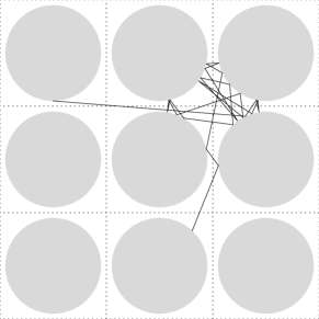
Figure 1: A trajectory in the infinite-horizon periodic Lorentz gas.

As is standard in billiard models, the dynamics may be studied either in discrete time or continuous time. The former is referred to as the billiard map, the latter as the billiard flow. The billiard map is restricted to the boundary of the billiard, and maps points with outgoing velocity from one collision to the next. The position at the $n$th collision will be denoted $\mathbf{r}_{n}$ and its velocity $\mathbf{v}_{n}$. Points under the billiard flow have position $\mathbf{r}(t)$ and velocity $\mathbf{v}(t)$ at continuous time $t$. Denoting the time of the $n$th collision by $t_{n}$, we thus have $\mathbf{r}(t_{n})=\mathbf{r}_{n}$, while, for $t_{n}<t<t_{n+1}$, $\mathbf{r}(t)$ is a point on the straight line joining $\mathbf{r}_{n}$ and $\mathbf{r}_{n+1}$, such that $\mathbf{r}(t)=\mathbf{r}_{n}+(t-t_{n})\mathbf{v}_{n}$. Correspondingly, the velocity $\mathbf{v}(t)$ remains unchanged until the next collision, $\mathbf{v}(t)=\mathbf{v}_{n}$. Due to the existence of open corridors, particles may propagate arbitrarily far without collision, so that the ballistic segments that connect successive collisions $\mathbf{r}_{n}$ and $\mathbf{r}_{n+1}$ are unbounded.

II Convergence to asymptotic behavior

We are interested in asymptotic transport properties, i.e., in the distribution of the displacement vector $\mathbf{r}(t)-\mathbf{r}(0)$ in the limit $t\to\infty$. In the remainder we shorten the notation and denote the displacement vector simply by $\mathbf{r}(t)$ as no confusion will arise. The modulus of this quantity will be denoted by $r(t)$.

II.1 Convergence in distribution

For the discrete-time dynamics, it has been proved Szász and Varjú (2007); Dolgopyat and Chernov (2009) that the displacement vector distribution with anomalous rescaling converges in distribution to a centered normal distribution: that is, as $n\to\infty$,

$$\frac{\mathbf{r}_{n}}{\sqrt{n\log{n}}}\to_{\mathrm{d}}\mathcal{N}(0,\Xi_{\mathrm{disc}}),$$ (2)

which means that the probability that the quantity in the left-hand side lies in a regular set $K$ converges to the probability that a normally-distributed random variable with mean $0$ and variance matrix $\Xi_{\mathrm{disc}}$ lies in $K$.

The covariance matrix $\Xi_{\mathrm{disc}}$ is a multiple of the identity matrix, i.e., its entries are given by $(\Xi_{\mathrm{disc}})_{i,j}=\xi_{\mathrm{disc}}\delta_{i,j}$. The discrete-time limiting variance $\xi_{\mathrm{disc}}$ is expressed in terms of the geometrical parameters of the model in Sec. III.

The corresponding result for the continuous-time flow was proved in Bleher (1992); Dolgopyat and Chernov (2009), and states the following: as $t\to\infty$,

$$\frac{\mathbf{r}(t)}{\sqrt{t\log t}}\to_{\mathrm{d}}\mathcal{N}(0,\Xi_{\mathrm{flow}}),$$ (3)

where $(\Xi_{\mathrm{flow}})_{i,j}=\xi_{\mathrm{flow}}\,\delta_{i,j}$ and $\xi_{\mathrm{flow}}=\xi_{\mathrm{disc}}/\tau_{\mathrm{MFT}}$. Here, $\tau_{\mathrm{MFT}}$ is the mean free time between collisions, which is proportional to the available area in the unit cell, $1-\pi\rho^{2}$, divided by the perimeter of the boundary, $2\pi\rho$ Chernov (1997):

$$\tau_{\mathrm{MFT}}=\frac{1-\pi\rho^{2}}{2\rho}.$$ (4)

II.2 Asymptotic behavior of moments

A standard method to characterize convergence of random variables numerically is via their moments. It is important to note, however, that convergence in distribution of a sequence of random variables to a limiting distribution does not necessarily imply convergence of the moments of the sequence to the moments of the limiting distribution.

Indeed, Armstead et al. Armstead et al. (2003) showed that the moments have dominant behavior:

$$\langle r(t)^{q}\rangle\sim\begin{cases}t^{q/2},&q<2,\\ t,&q=2,\\ t^{q-1},&q>2,\end{cases}$$ (5)

ignoring logarithmic corrections; see also Ref. Artuso and Cristadoro (2003). A proof of the result for $q>2$ has recently been announced Melbourne and Török (2011); Melbourne (2012).

The type of qualitative change in the scaling of the moments seen in Eq. (5) has elsewhere been dubbed strong anomalous diffusion Castiglione et al. (1999), as opposed to weak when a single exponent ($\neq 1/2$) characterizes the whole spectrum of moments. It appears to be typical for anomalous transport arising from deterministic dynamical systems Artuso and Cristadoro (2003), as opposed to the single scaling of the converging moments for self-similar stable distributions Gnedenko and Kolmogorov (1968). Such behavior is due to the fact that the slowly-decaying tail of the displacement vector distribution may give no contribution to the convergence in distribution of the rescaled variable, while nonetheless playing a dominant role for sufficiently high moments.

We denote by $M_{q}$ the $q$th moment of the limiting two-dimensional normal distribution (3):

$$M_{q}\equiv\Gamma\left(1+\tfrac{q}{2}\right)\,(2\xi_{\mathrm{flow}})^{q/2},$$ (6)

where $\Gamma$ is the Gamma function. If the convergence in (3) were sufficiently strong, then the $q$th moment of the rescaled displacement vector distribution would converge to $M_{q}$, for all $q$. In fact, however, the weak convergence (3) implies this convergence of the moments only for $q<2$ (Knight, 2000, Sec. 3.2):

$$\left\langle\left[\frac{r(t)}{\sqrt{t\log t}}\right]^{q}\right\rangle\to M_{q}\qquad(q<2),$$ (7)

when $t\to\infty$. For $q>2$ this does not hold, and the asymptotic values of the $q$th moments of the rescaled displacement vector distribution diverge, as follows from (5).

The case $q=2$ requires special consideration. If Eq. (7) applied in this case, we would have the asymptotic behavior $\langle r(t)^{2}\rangle/(t\log t)\sim 2\xi_{\mathrm{flow}}$. However, this is incorrect: it has recently been discovered that in fact an extra factor of $2$ appears, so that the correct asymptotic behavior is

$$\frac{1}{2t}\left\langle r(t)^{2}\right\rangle\sim 2\xi_{\mathrm{flow}}\log t.$$ (8)

An explanation of this phenomenon was given in Ref. Dettmann (2012), and a proof has been announced Chernov et al. (2012). A similar result appears also in a different setting; see Ref. Bálint et al. (2011), where a rigorous argument is available for a related billiard model with cusps. This surprising behavior is due to the fact that the contribution to the second moment (8) of collisionless orbits is equal to that coming from the central part of the distribution, while playing no role in the weak convergence to a normal distribution in Eq. (3).

We note that there has been recent interest in the extension of these results to higher-dimensional Lorentz gases Sanders (2008); Dettmann (2012); Nándori et al. (2012), where additional effects come into play.

III Corridors and variance of limiting distribution

Before turning to numerical measurements of the asymptotic behaviors (7) and (8) in the next section, we consider the computation of the variance of the limiting distribution (3).

As proved in Dolgopyat and Chernov (2009), the general expression for the discrete-time limiting covariance matrix $\Xi_{\mathrm{disc}}$ is

$$(\Xi_{\mathrm{disc}})_{i,j}=\frac{c_{\nu}}{2}\sum_{x}\frac{w_{x}^{2}\,\psi_{i}(x)\psi_{j}(x)}{|\boldsymbol{\psi}(x)|},$$ (9)

where the sum runs over all fixed points $x$ of the collision map on the unit cell, of which there are four for each corridor. Here $w_{x}$ is the width of the corresponding corridor and $\boldsymbol{\psi}(x)$ is the vector of Cartesian components $\psi_{i}(x)$ ($i=1,2$) parallel to the corridor, giving the translation in configuration space described by the action of the map on $x$ , and $c_{\nu}=1/(4\pi\rho)$ is a normalizing constant. It follows from the symmetries of the system that the non-diagonal elements of the covariance matrix vanish.

Given the parameter value $\rho$, Eq. (9), along with an enumeration of all the fixed points of the collision map, allows one to write the expression for the discrete-time limiting variance $\xi_{\mathrm{disc}}$. By including the mean free time (4), the corresponding expression for the continuous-time limiting variance $\xi_{\mathrm{flow}}$ may then be obtained.

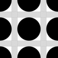
(a)  Type $(0,1)$ ($\rho=0.4$).

(b)  Type $(1,1)$ ($\rho=0.3$).

(c)  Type $(1,2)$ ($\rho=0.2$).

Figure 2: Examples of infinite-horizon corridors in the periodic Lorentz gas, labelled according to their type $(m,n)$; see text for details.

When $1/(2\sqrt{2})\leq\rho<1/2$, the only corridors present are horizontal and vertical corridors of width $w=1-2\rho$, which we refer to as type $(0,1)$ corridors; see Fig. 2(a). $\xi_{\mathrm{flow}}$ then has the only contribution

$$\frac{(1-2\rho)^{2}}{\pi(1-\pi\rho^{2})}.$$ (10)

When $1/(2\sqrt{5})\leq\rho<1/(2\sqrt{2})$, two new corridors, of type $(1,1)$, open up, along the vectors $(1,\pm 1)$, with width $w=1/\sqrt{2}-2\rho$; see Fig. 2(b). Their contribution to $\xi_{\mathrm{flow}}$ is

$$\frac{1}{\pi(1-\pi\rho^{2})}\sqrt{2}\Big{(}\frac{1}{\sqrt{2}}-2\rho\Big{)}^{2}.$$ (11)

Additional corridors keep appearing as $\rho$ decreases. By symmetry, they all occur in quadruplets. For instance, the type $(1,2)$ corridors, which appear when $\rho<1/(2\sqrt{5})$, are shown in Fig. 2(c); they point along the vectors $(1,\pm 2)$ and $(2,\pm 1)$ and have width $w=1/\sqrt{5}-2\rho$.

The general expression of the limiting variance is

$$\xi_{\mathrm{flow}} =\frac{1}{\pi(1-\pi\rho^{2})}\bigg{[}(1-2\rho)^{2}+\sqrt{2}\Upsilon\Big{(}\frac{1}{\sqrt{2}}-2\rho\Big{)}$$ (12)

$$\quad+2\sum_{m=1}^{\infty}\sum_{\begin{subarray}{c}n=m+1:\\ \mathrm{gcd}(m,n)=1\end{subarray}}^{\infty}\sqrt{m^{2}+n^{2}}\,\,\Upsilon\Big{(}\frac{1}{\sqrt{m^{2}+n^{2}}}-2\rho\Big{)}\bigg{]},$$

where $\Upsilon(x)=x^{2}$ if $x>0$, and $0$ otherwise and $\mathrm{gcd}(m,n)$ denotes the greatest common divisor of $m$ and $n$; the sum thus runs over all pairs of relatively prime integers $m$ and $n$ such that $1\leq m<n$. The number of contributions to $\xi_{\mathrm{flow}}$ depends on the radius $\rho>0$, and is always finite. For example, for $\rho=0.2$, there are three types of corridors open, depicted in Fig. 2.

IV Numerical measurements of the moments

We study the behavior of the moments of the distribution of the anomalously-rescaled process $\mathbf{r}(t)/\sqrt{t\log t}$, relating our numerical results to the parameters of its limiting normal distribution such as $\xi_{\mathrm{flow}}$, Eq. (12), which, for simplicity, we will henceforth refer to as the variance.

IV.1 Time-dependence of the first and second moments

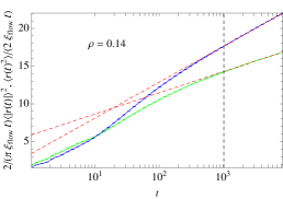
(a)  1st and 2nd moments, $\rho=0.14$

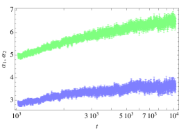
(b)  Intercepts, $\rho=0.14$

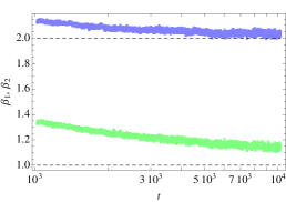
(c)  Slopes, $\rho=0.14$

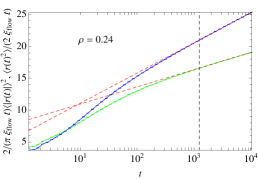
(d)  1st and 2nd moments, $\rho=0.24$

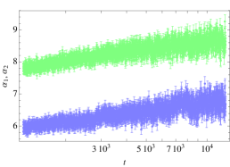
(e)  Intercepts, $\rho=0.24$

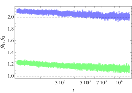
(f)  Slopes, $\rho=0.24$

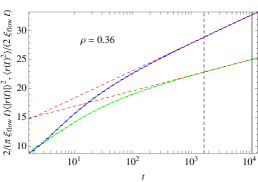
(g)  1st and 2nd moments, $\rho=0.36$

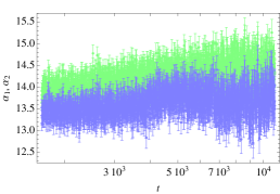
(h)  Intercepts, $\rho=0.36$

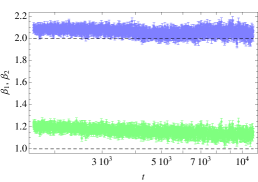
(i)  Slopes, $\rho=0.36$

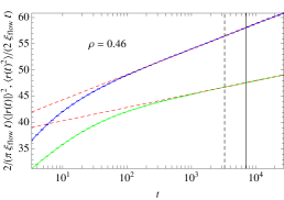
(j)  1st and 2nd moments, $\rho=0.46$

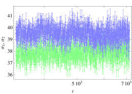
(k)  Intercepts, $\rho=0.46$

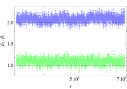
(l)  Slopes, $\rho=0.46$

Figure 3: (Color online) Left panels: numerical measurements of the normalized first (green, bottom curves) and second (blue, top curves) moments, Eqs. (13)-(14), as functions of time. The dashed red lines show the results of linear fits of these two curves, i.e., as affine functions of $\log t$, computed in the interval delimited by the two vertical lines; see Sec. IV.3 for further details. Middle and right panels: graphs of the measured intercepts, $\alpha_{i}$, and slopes, $\beta_{i}$, $i=1,2$, of the normalized moments as functions of time, i.e., obtained by fitting straight lines through successive pairs of data points. The time-ranges of those graphs correspond to the fitting intervals shown on the left panels. The number of open corridor types is four for the parameter value $\rho=0.14$, Figs. 3(a)-3(c), two for $\rho=0.24$, Figs. 3(d)-3(f), and one for $\rho=0.36$ and $0.46$, Figs. 3(g)-3(l).

We focus on the first two moments of the rescaled displacement vector. We are particularly interested in the second moment for its physical relevance, but also because the exponent $q=2$ is the onset of the anomalous behavior, Eq. (5). For further validation of our results, we provide a comparison between the second and the first moments. As discussed earlier, we need to critically assess the effect of finite-time measurements of these quantities; the important point to notice is that the “large” times that are needed to observe the asymptotics of Eqs. (7)-(8) must be understood as logarithmically large times, i.e., times so large that their logarithm is actually large.

Higher moments, $q>2$, will not be analyzed here. For these moments, it is believed that logarithmic corrections to the scaling (5) are in fact absent Melbourne (2012). Their measurement is, however, delicate Zaslavsky and Edelman (1997); Courbage et al. (2008); we will return to this issue in a separate publication.

Following the discussion in Sec. II.2, we measure numerically the left-hand side of Eq. (8), which, up to a numerical factor, is proportional to the finite-time diffusion coefficient $D(t)$, Eq. (1). However, as detailed in the introduction, to obtain an accurate measurement of the logarithmic divergence of this quantity, it is necessary to include terms of order $1$ in this expression. (We do not include terms of order between $1$ and $\log t$, as they would be invisible to our simulations.) Dividing by the variance so as to eliminate the dependence on the model’s parameter from the asymptotic result (8), we thus seek an asymptotically affine function of $\log t$:

$$\frac{1}{2\xi_{\mathrm{flow}}t}\left\langle r(t)^{2}\right\rangle\sim\alpha_{2}+\beta_{2}\log t,$$ (13)

where $\alpha_{2}$ and $\beta_{2}$ are implicit functions of time, and are expected to converge to constant values as $t\to\infty$; according to Eq. (8), we should find $\beta_{2}=2$ for large enough times.

In contrast to the second moment, the first moment (of the norm of the displacement vector) must follow Eq. (7). Taking the square of this quantity and dividing by the variance, we again expect an asymptotically affine function of $\log t$:

$$\frac{2}{\pi\xi_{\mathrm{flow}}t}\big{\langle}r(t)\big{\rangle}^{2}\sim\alpha_{1}+\beta_{1}\log t,$$ (14)

now with $\beta_{1}=1$ for large enough times.

We refer to the quantities on the left-hand side of Eqs. (13)-(14) as the normalized second and first moments respectively.

Examples of numerical computations of these quantities are provided in Fig. 3, for different parameter values. The left panels display the graphs of these two normalized moments as functions of time, on logarithmic scales. For times large enough, the curves tend to straight lines whose fits provide estimates of the coefficients $\alpha_{i}$ and $\beta_{i}$, shown as functions of time on the middle and right panels, respectively; see Sec. IV.3 for further details on the computation of these coefficients.

As evidenced by the data shown in Fig. 3, when the linear interpolation is performed on a (logarithmically) small neighborhood of some given finite time $t$, we must think of all four fitting parameters as functions of $t$. Since the asymptotic convergences in Eqs. (7)-(8) occur over a logarithmic time scale, it is reasonable to expect a slow convergence of these quantities; the deviations of the measured coefficients $\alpha_{i}$ and $\beta_{i}$ from their asymptotic values are indeed found to decay as power laws with exponents less than one; see the discussion below.

Let us remark once again that there are in general no analytical predictions for the fitting parameters $\alpha_{i}$. Though the slopes $\beta_{i}$ ($i=1,2$) are asymptotically independent of the model’s parameter $\rho$, this is not expected of the intercepts $\alpha_{i}$; using dimensional arguments, it is in fact not difficult to convince oneself that $\alpha_{i}$ should diverge with $1/(1-2\rho)$ as $\rho\to 1/2$. In other words, $\alpha_{i}\gg\beta_{i}$ in the limit of narrow corridors. At times $t$ attainable in numerical simulations we should thus typically expect the intercepts to be of sizes similar to the terms $\beta_{i}\log t$ on the right-hand sides of Eqs. (13)-(14), or even much larger, as occurs when $\rho\to 1/2$; this regime will be analyzed in a separate publication Cristadoro et al. (a).

We believe this observation is key to explaining the difficulties met in observing numerically the asymptotic scalings in Eqs. (7)-(8). Recognizing that short time averages tend to be dominated by diffusive motion helps explain the relevance of the fitting parameters $\alpha_{i}$. Indeed the effect of ballistic trajectories on the statistics of displacements is feeble and the anomalous logarithmic divergences have a rather weak influence on the finite-time statistics, especially so when $\rho$ is close to its upper bound, $1/2$ (so that the horizontal and vertical corridors have narrowing widths).

IV.2 Time span of measurements

For a given value of the parameter $\rho$, a key issue is to determine a time interval where the fitting parameters $\alpha_{i}$ and $\beta_{i}$ in Eqs. (13)-(14) can be accurately measured. As discussed in the introduction, integration times should be neither too short, nor too long; they should be large enough to avoid the regime where transient effects dominate, but cannot be too large, since the number of initial conditions required to sample the moments up to a given time scale grows with the square of this scale; see the discussion below.

At the level of the dynamics, there are distinct time scales at play. The first is the mean free time, $\tau_{\mathrm{MFT}}$, Eq. (4), which measures the average time that separates successive collisions with scatterers.

To identify a second timescale, which characterizes the motion of a point particle on the billiard table, consider a lattice of unit cells each shifted by one half of a unit length in both vertical and horizontal directions, so that obstacles are now sitting at the cells’ corners rather than at their centers. The average time it takes for a particle at unit speed to exit a cell after it entered it (with position and velocity distributed according to the Liouville measure for the Poincaré section given by the four line segments delimiting each cell) is Chernov (1997)

$$\tau_{\mathrm{R}}=\frac{\pi(1-\pi\rho^{2})}{4(1-2\rho)}.$$ (15)

The residence time $\tau_{\mathrm{R}}$ provides a natural time unit of lattice displacements. Note that, whereas $\tau_{\mathrm{MFT}}$, Eq. (4), diverges in the limit of small scatterers, $\rho\to 0$, $\tau_{\mathrm{R}}$ diverges in the opposite limit of narrow corridors, $\rho\to 1/2$.

In the presence of infinite corridors, the other relevant timescale is of course the ballistic one, which, for horizontal and vertical corridors, is, in the units of cell sizes and speed of point particles,

$$\tau_{\mathrm{B}}=1.$$ (16)

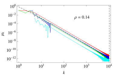
(a)  Distribution of ballistic segments, $\rho=0.14$

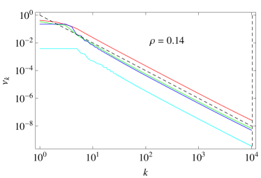
(b)  Cumulative distribution of ballistic segments, $\rho=0.14$

Figure 4: (Color online) Numerical measurements of the distributions of the ballistic segments for the parameter value $\rho=0.14$. Four different types of corridors are open: $(1,0)$ (red curve), $(1,1)$ (green curve), $(1,2)$ (blue curve), and $(1,3)$ (cyan curve). The black dashed curves are defined according to Eqs. (17)-(18), respectively, and have the same asymptotics.

As can be seen in Fig. 3, the initial regime, which is dominated by transient effects, is typically longer for the first moment than the second. For either moment, however, the lengths of transients may depend on several factors, such as the persistence of correlations, or the precise distribution of ballistic segments, which vary with the parameter’s value. Moreover, in an idealized model such that ballistic segments are independent and identically distributed (so that correlations are absent) $\alpha_{i}$ and $\beta_{i}$ display $1/t$ corrections to their asymptotic values Cristadoro et al. (b). For the billiard dynamics, we should a fortiori expect a decay not faster than $1/t$; the convergence to the asymptotic regime might be even slower.

The distinction between the initial transient regime and that where the moments follow Eqs. (13)-(14), with fitting parameters displaying small finite-time corrections, is not sharp. There is in fact no easy way to estimate the length of the initial transient regime, a priori. Empirically, however, we find the initial regime to subdue after a duration between $10^{3}$ and $10^{4}$ units of $\tau_{\mathrm{MFT}}$, which, in the range of parameter values $\rho$ investigated, may thus vary from several hundred units of $\tau_{\mathrm{R}}$ to a few thousand, depending on the value of the parameter.

Integration times should therefore be greater than a few thousand units of $\tau_{\mathrm{R}}$. How much greater depends on one’s ability to sample ballistic segments over that duration. Since it is known Szász and Varjú (2007) that the distribution of the lengths of ballistic segments in infinite-horizon periodic Lorentz gases decays with the cube of their lengths,

$$\mu_{k}\sim\frac{1}{k^{3}},$$ (17)

let us compare our numerical findings to the following model for the corresponding cumulative distribution, by which we mean the probability of having ballistic segments of lengths at least $k$,

$$\nu_{k}=\sum_{j=k}^{\infty}\mu_{j}=\frac{1}{k^{2}}.$$ (18)

Incidentally, $\nu_{1}=1$ is equivalent to normalization of the probabilities (17), for $k$ ranging over positive integers. The $k^{2}$ decay in the above equation is responsible for the logarithmic divergence of the normalized second moment.

Now, suppose that, for times up to $k$, we want to accurately sample ballistic segments of lengths $k$—assuming that this will imply a good sampling of shorter ballistic segments as well. Since point particles have unit speed, the flights of lengths $k$ cannot experience a collision in the time interval $[0,k]$ (modulo corrections that are negligible for large $k$). They are thus indistinguishable, in the time-frame considered, from flights of lengths $\geq k$, as we do not know when the last collision before time 0 occurred or when the first one after time $k$ will. So we must consider the entire set of ballistic segments of lengths $\geq k$, whose probability is given by (18), as a whole, and each segment there will contribute with a length $k$, in the time interval $[0,k]$. Accordingly, the number of initial conditions we have to sample in order to accurately measure the moments for times up to $k$ grows like $k^{2}$.

The tails of the actual distributions of ballistic segments, shown in Fig. 4 for $\rho=0.14$, differ from Eqs. (17)-(18) by a numerical factor which is $\mathcal{O}(1-2\rho)$. In the narrow corridor limit, transitions between cells are overwhelmingly dominated by segments of unit lengths; ballistic segments are thus infrequent. Away from this limit, however, ballistic trajectories occur at manageable frequencies.

Considering the examples displayed in Fig. 3, the initial transient regime subdues after times roughly $t\sim 10^{4}$. For the parameter values shown, and up to a constant factor of order unity , the cumulative distribution of ballistic segments is well approximated by Eq. (18), at least for $k\gg 1$. We thus typically need $10^{8}$ initial conditions to sample trajectories up to time $t\sim 10^{4}$, but would need $10^{10}$ initial conditions to sample trajectories for times up to $t\sim 10^{5}$. While the former is within reach of our numerical computations, the latter is not, at least not unless one is able to devote about ten years’ worth of CPU time to it, notwithstanding the impact of the limited accuracy of the integration on the results.

Statistical averages are, in practice, limited to ensembles of at most a billion trajectories of duration $10^{4}\tau_{\mathrm{R}}$. The margin between the decay of initial transients and the largest timescale for which ballistic trajectories are accurately sampled is thus typically narrow.

IV.3 Details of the numerical procedure and results

$\rho$	$t_{\mathrm{tot}}$	$t_{\mathrm{f}}$	$N$	$\alpha_{1}$	$\beta_{1}$	$\alpha_{2}$	$\beta_{2}$
$0.14$	$1.02\times 10^{5}$	$1.65\times 10^{4}$	$240$	$6.8\pm 0.6$	$1.11\pm 0.06$	$3.8\pm 0.5$	$2.02\pm 0.05$
	$1.02\times 10^{4}$	$1.02\times 10^{4}$	$1440$	$6.50\pm 0.02$	$1.142\pm 0.002$	$3.67\pm 0.07$	$2.029\pm 0.007$
$0.24$	$1.24\times 10^{4}$	$1.24\times 10^{4}$	$1000$	$8.58\pm 0.08$	$1.135\pm 0.009$	$6.68\pm 0.02$	$2.0059\pm 0.0007$
$0.36$	$1.66\times 10^{4}$	$1.10\times 10^{4}$	$1000$	$14.33\pm 0.03$	$1.152\pm 0.003$	$13.54\pm 0.05$	$2.069\pm 0.005$
$0.46$	$3.29\times 10^{4}$	$7.16\times 10^{3}$	$1200$	$37.8\pm 0.7$	$1.10\pm 0.08$	$39.8\pm 0.6$	$2.11\pm 0.06$
	$3.29\times 10^{3}$	$3.29\times 10^{3}$	$1100$	$37.44\pm 0.06$	$1.150\pm 0.008$	$40.24\pm 0.05$	$1.994\pm 0.007$

Table 1: Numerical measurements of the fitting parameters $\alpha_{i}$ and $\beta_{i}$, $i=1,2$, of the normalized moments (13)-(14) for different values of the model’s parameter, $\rho$. For each parameter value, we indicate $t_{\mathrm{tot}}$, the total integration time, $t_{\mathrm{f}}$ the largest time in the fitting range, and $N$, the number of groups of $10^{6}$ trajectories used to gather the corresponding data. The values of the coefficients $\alpha_{i}$ and $\beta_{i}$, $i=1,2$ reported here are obtained by computing the means and their standard deviations for measurement times $t$ near $t_{\mathrm{f}}$.

Numerical integration of trajectories on the infinite-horizon Lorentz gas proceeds according to standard event-driven algorithms, which are common to systems with hard-core interactions Lubachevsky (1991). A specificity, however, is in the choice of initial conditions, which are sampled from the standard Liouville distribution along the vertical and horizontal borders of a unit cell. This choice allows to sample trajectories initially in the process of completing a ballistic segment, as part of the equilibrium distribution; such trajectories would be absent from the statistical ensemble had we instead chosen to distribute initial conditions on the surface of the obstacle, i.e., where collision events take place.

Each trajectory is integrated over a given time span $t_{\mathrm{tot}}$, during which the particle’s position on the billiard table is regularly sampled, at intervals of time uniformly distributed on a logarithmic scale. Statistical averages of observables such as the normalized moments (13)-(14) are obtained by repeating measurements of these quantities for a large number of initial conditions.

As integration proceeds, the distribution of ballistic segments is computed by recording successive ballistic segments, according to their lengths and corridor types, see Fig. 4(a). At the end of the integration, we obtain a criterion for determining an upper bound $t_{\mathrm{f}}$, of the times up to which statistical averages are reliably computed: we choose $k_{\mathrm{f}}$ to be the smallest integer $k$ such that the percentage of unsampled ballistic segments of lengths $\leq k$ exceeds $0.1\%$. Finally we set $t_{\mathrm{f}}=k_{\mathrm{f}}$, as speed is fixed to one. On the left panels of Fig. 3, $t_{\mathrm{f}}$ is marked by vertical solid lines. Of course, this is but a rough way of estimating the largest ballistic scale such that the cumulative distribution of ballistic segments is accurately sampled. Though it may not be optimal, this is a quantitative criterion that has, among its advantages, that it is easy to implement and requires no a priori knowledge of the distribution of ballistic segments.

In Fig. 3, the lower bounds of the fitting intervals, marked by solid vertical lines on the left panels, are taken to be one tenth of the total integration time of the simulation, $t_{\mathrm{i}}\equiv t_{\mathrm{tot}}/10$, which we set to $t_{\mathrm{tot}}\equiv 10^{4}\tau_{\mathrm{R}}$. The bounds $t_{\mathrm{i}}$ and $t_{\mathrm{f}}$ also correspond to the time ranges of the figures shown on the middle and right panels of Fig. 3. The data themselves are obtained by computing the averages of the normalized first and second moments (13)-(14) as functions of time for about one thousand groups of $10^{6}$ trajectories each; see Table 1 for details. The times $\{t_{k}\}_{k=1}^{N}$, at which the moments are computed, span $N=10^{4}$ sub-intervals of $t_{\mathrm{tot}}$, such that $t_{k}/t_{k-1}=N^{1/N}$ and $t_{N}=t_{\mathrm{tot}}$.

Having determined fitting intervals by inspection of the distributions of ballistic segments according to the criterion described above, we compute, for each measurement time $t_{k}$ within the fitting interval, $t_{\mathrm{i}}\leq t_{k}\leq t_{\mathrm{f}}$, the values of the fitting parameters $\alpha_{i}$ and $\beta_{i}$ of the normalized moments averaged over a group of $10^{6}$ trajectories. This is achieved by fitting straight lines through successive pairs of data points, at $t_{k}$ and $t_{k+1}$. Since the measurement times are spread uniformly on a logarithmic scale, we obtain in this way, for the set of measurement times $t_{k}$ in the interval between $t_{\mathrm{i}}$ and $t_{\mathrm{f}}$, sequences of values of $\alpha_{i}$ and $\beta_{i}$, whose means (for the corresponding measurement times $t_{k}$) are displayed on the middle and right panels of Fig. 3. The standard deviations of these means yield the corresponding error bars.

In Table 1, we extracted from Fig. 3 the values of the fitting parameters $\alpha_{i}$ and $\beta_{i}$, measured at the right-ends of the fitting intervals. The precision reported on those values reflect the fluctuations observed over the last ten data points of each of the fitting intervals. Increasing the time span would clearly result in smaller error bars. It must however be assumed that the fitting parameters do not exhibit significant time dependence over the chosen time span.

Integration times vary with the value of the model’s parameter $\rho$. For small values of $\rho$ it is possible to take longer integration times, with large enough numbers of initial conditions. On the contrary, when $\rho$ increases towards $1/2$, integration times have to be decreased in order to allow for large enough numbers of initial conditions. For $\rho=0.14$, we also report in Table 1 values of the fitting parameters obtained by integrating over a total time of $10^{5}\tau_{\mathrm{R}}$. The width of the fitting interval is thus larger than that obtained by integrating over times $10^{4}\tau_{\mathrm{R}}$, but only by a small factor; accordingly, the values of the fitting parameters do not vary appreciably.

At the opposite end of the range of parameter values shown here, for $\rho=0.46$, though the number of initial conditions reported for integration times up to $10^{4}\tau_{\mathrm{R}}$ is rather large, the precision on the fitting parameters is not as good, particularly for $\beta_{2}$; this is also reflected by the fluctuations observed in the data displayed in Fig. 3(l). Repeating the measurement over a total integration time of $10^{3}\tau_{\mathrm{R}}$, we obtain better statistics for comparable fitting times.

Overall, the convergence of $\beta_{2}$ to its asymptotic value, $2$, is observed with better accuracy than that of $\beta_{1}$ to $1$. The values obtained are consistent throughout the range of the model’s parameter values, in spite of the variations in the values of the intercepts, $\alpha_{1}$ and $\alpha_{2}$. We interpret this as a clear vindication of our methods; weak logarithmic divergences of the mean-squared displacements of point-particles on infinite-horizon billiard tables can be measured with satisfactory precision, regardless of their strength, gauged by the variance $\xi_{\mathrm{flow}}$, Eq. (12).

V Conclusions

The periodic Lorentz gases on a square lattice investigated in this paper are prototypical examples of infinite-horizon billiard tables, exhibiting a weak from of super-diffusion. Such a regime is marginal in the sense that it lies at the border between regimes of normal diffusion and regimes of anomalous super-diffusion with mean-squared displacement growing with a power of time strictly greater than unity.

In the case of our “weak super-diffusion”, corrections to the linear growth of the mean-squared displacement are logarithmic in time. For moderately large times, i.e., those times which are accessible to numerical computations, the slow growth of these corrections implies the coexistence of two distinct regimes, one of normal diffusion, whereby point-particles move short distances between collisions with obstacles, i.e., of order of the inter-cell distance, and, the other, a regime of accelerated (also termed enhanced) diffusion due to the presence of ballistic trajectories.

Though the asymptotic regime—that which exhibits the logarithmic divergence—has been well understood on a rigorous level, much less can be said about the regime of normal diffusion with which it typically coexists. As argued in this paper, ignoring this second regime ultimately masks the asymptotic regime itself, precluding its accurate detection. In this respect, a great deal can be learned from a careful numerical investigation.

The analysis presented in this paper has focused on two moments of the normalized displacement, each with distinct characteristics. On one hand, the first moment (of the modulus) of the displacement vector was taken as a benchmark of the limit law (7), for which we could check the convergence of the corresponding moment of the anomalously rescaled process. Though this convergence could be verified with good accuracy throughout the range of the model’s parameter values we investigated, it must be noted that it appears to be slower in the regime of large corridors than in the opposite regime, of narrow corridors.

The second moment, on the other hand, is of particular importance because it marks the onset of the anomalous scaling regime (5). As noted, the corresponding moment of the anomalously rescaled process is expected to converge to twice its limiting variance. This observation is indeed consistent with numerical measurements of this quantity, to within very good accuracy in most cases.

The numerical investigations reported in this paper are based on standard event-driven algorithms, with uniform sampling of trajectories. No attempt was made to use special techniques to improve the sampling of ballistic trajectories. Further investigations will focus on refined algorithms specifically designed to explore phase-space regions associated with such rare events, e.g., in the spirit of Refs. Hsu and Grassberger (2011); Laffargue and Tailleur (2014); Leitão et al. (2013), and assess their usefulness for the sake of computing statistical averages.

A separate perspective relates to the connection between infinite Lorentz gases and stochastic processes. The infinite-horizon Lorentz gas can indeed be viewed as an example of a correlated Lévy walk, whose distribution of free paths scales with the inverse cubic power of their lengths. Models of such walks appear in the context of random search algorithms Viswanathan et al. (2011). Better understood, however, are uncorrelated Lévy walks Geisel et al. (1985); Zumofen and Klafter (1993). In this context scalings of the mean-squared displacement such as Eq. (1) are known to occur when the free paths are distributed as in Eq. (17). In a separate publication, we will show that the narrow corridor limit of the infinite-horizon Lorentz gas is a fertile study ground for a class of such walks, where both normal and anomalous diffusion coexist. Much in the spirit of the Machta-Zwanzig approximation to the diffusion coefficient of normally diffusive finite-horizon periodic billiard tables Machta and Zwanzig (1983), correlations between successive ballistic segments die out as the narrow corridors limit is reached. In this limit, the terms of order $1$ in the normalized moments take on a simple dimensional form which plainly justifies the contrast between the coexistence of normally and anomalously diffusive contributions in the finite-time expression of the mean-squared displacement. To describe this limit in an appropriate framework, we will introduce a description in terms of continuous time random walks with delay. As it turns out, this is but a particular case of a much larger class, which includes models with all diffusive regimes, ranging from sub- to super-diffusive. The details will be reported elsewhere.