Trimer superfluid induced by photoassocation on the state-dependent optical lattice

Abstract

We use the mean-field method, the Quantum Monte-carlo method and the Density matrix renormalization group method to study the trimer superfluid phase and the quantum phase diagram of the Bose-Hubbard model in an optical lattice, with explicit trimer tunneling term. Theoretically, we derive the explicit trimer hopping terms, such as $a_{i}^{3\dagger}a_{j}^{3}$, by the Schrieffer-Wolf transformation. In practice, the trimer superfluid described by these terms is driven by photoassociation. The phase transition between the trimer superfluid phase and other phases are also studied. Without the on-site interaction, the phase transition between the trimer superfluid phase and the Mott Insulator phase is continuous. Turning on the on-site interaction, the phase transitions are first order with Mott insulators of atom filling $1$ and $2$. With nonzero atom tunneling, the phase transition is first order from the atom superfluid to the trimer superfluid. In the trimer superfluid phase, the winding numbers can be divided by three without any remainders. In the atom superfluid and pair superfluid, the vorticities are $1$ and $1/2$, respectively. However, the vorticity is $1/3$ for the trimer superfluid. The power law decay exponents is $1/2$ for the non diagonal correlation $a_{i}^{\dagger 3}a_{j}^{3}$, i.e. the same as the exponent of the correlation $a_{i}^{\dagger}a_{j}$ in hardcore bosons. The density dependent atom-tunneling term $n_{i}^{2}a_{i}^{\dagger}a_{j}$ and pair tunneling term $n_{i}a_{i}^{\dagger 2}a_{j}^{2}$ are also studied. With these terms, the phase transition from the empty phase to atom superfluid is first order and different from the cases without the density dependent terms. The phase transition is still first order from the trimer superfluid phase to the atom superfluid. The effects of temperature are studied. Our results will be helpful in realizing the trimer superfluid by a cold atom experiment.

I Introduction.

In recent years, the Bose-Hubbard model using an on-site attractive interactionth1 ; 3bodyloss ; 3body2 ; mfy1 ; mfy2 ; psf ; ycc ; fintemp , or with explicit pair tunneling termxfzhou ; wz1 ; wz2 has caught the attention of theoretical and experimental physicists. As for atoms with a two-body attractive interaction on an optical lattice, bosons can form an interesting spontaneous pair-tunneling between two of the nearest neighbor sites. This motion forms a pair superfluid state (PSF) which is stabilized by a three-body constraint, even though the Hamiltonian has no obvious pair-tunneling term. The three-body constraint($a^{\dagger 3}=0$), e.g. two atoms allowed in a site, has been realized by large three-body loss processes3bodyloss ; 3body2 .

Besides the attraction-induced pair superfluid, virtually excited atom-pairs driven by atom-molecule coupling, could lead to a PSF. Compared with a spontaneous PSF, this artificially driven superfluid covers a larger parameter area in the phase diagram. So the PSF is more detectable in experiments and it is easier to explore the phase transition between a PSF and other phasesxfzhou ; wz1 ; wz2 .

Naturally, the question arises: can the trimer superfluid(TSF) exist in a stable fashion and be detectable in the real experiments? In the TSF phase, three atoms on one site will tunnel into the neighborhood sites simultaneously. An on-site trimer can exist by using a Bose gas on the optical lattice1st , in which two atoms are in the lowest hyperfine state, and the third atom sits in an excited hyperfine state. Other Bose trimers have been observed in the several few-body systems, such as 7Lili7 , 39K39K , 85Rb85Rb and 133Cs133Cs .

Evidence about an Efimov superfluidefimov ; efimovsf and trimer condensation in a frustrated systemzhaihui on the Kagome lattice shows that exploring the macroscopic behaviors of trimer tunneling, instead of small clusters, is a interesting topic in the cold atom regime. Actually, by loading the atoms into a state dependent latticexfzhou , the laser could drive the pair atoms tunnel on the optical lattice. In high densities, there is a possibility to form trimers as the collision occur between dimers and atoms by photoassociationPA . So it is possible to drive the trimers tunnel on the lattice and explore the TSF phase and other kinds of macroscopic behavior.

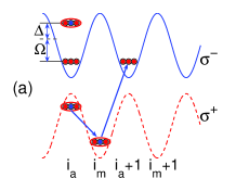
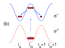
Figure 1: (Color online) (a) Experimental realization of trimer hopping in a state dependent optical lattice. $\Delta$ is the detuning parameter and $\Omega$ represents the atom-molecule coupling. The red and blue circles represent bosons in the lowest and (excited) hyperfine states, respectively. (b) The atom tunneling and pair tunneling in the procedure of trimer formation. The probability of a separation is smaller than the probability of the trimer formation.

In the present work, we provide a model with trimer hopping terms and additional new terms analytically and the possibilities of various ratios of the parameters. We actively find the TSF on the state-dependent optical lattice, in certain parameter regions. The phase transition between the trimer superfluid and other phases are also studied. The typical distribution of winding numbers are shown with the vorticity of the TSF phase being $1/3$. The power law decay exponents of the correlation are discussed as well the effects of density dependent tunneling are studied. The finite-temperature phase diagrams are provided both with and without the atom tunneling.

The outline of this work is as follows. Sec. II shows the derivation of the model, the controllable range of the parameters, and the experimental realization. We describe the methods and useful observables in Sec. III. We then present the ground state phase diagram and the TSF phase, in Sec. IV, for various cases. The winding numbers and correlations are also discussed. Sec. V shows the effects of density dependent terms. In particular, we show the first-order transition between the empty phase and the atom superfluid (ASF) phase. The first-order transition of ASF-TSF is also shown. Sec. VI focusses on the finite-temperature properties of the TSF phase. Concluding comments are made in Sec. VII.

II The model

II.1 Experimental realization of trimer tunneling

Figure 1(a) shows a possible path for the trimer tunneling on the state dependent lattice. This scheme is different from the one described in previous work1st , which uses the usual optical lattice. We make the initial three free ⁷Li ${}^{2}S_{1/2}$ atoms sit in the well $i_{a}$. We excite one of the three atoms to state ${}^{2}P_{3/2}$ by photoassociation with the $\sigma^{+}$ laser instead of the $\pi$ laserphotoasso , and then the three atoms form the ${}^{2}P_{3/2}+^{2}S_{1/2}+^{2}S_{1/2}$ trimer. By modulating the relative depth of the $\sigma^{\pm}$ potential, the effective potential is obtained as illustrated by a dashed line in the figures. The trimer tunnels to site $i_{m}$, and then emission spontaneously occurs towards the ${}^{2}S_{1/2}+^{2}S_{1/2}+^{2}S_{1/2}$ atoms on site $i_{m}$. Similarly, just by “feeling” the local maximum of the potential of the $\sigma^{-}$ laser, as illustrated by a solid line, the trimer tunnels into site $i_{a}+1$. Figure 1(b) shows that the atoms in the trimer can possibly separate and tunnel into sites with different directions. However, the probability of a separation is smaller than the trimer tunneling.

II.2 Theoretical derivation

The interactions of the whole system are of three types: atom-atom, atom-trimer, and trimer-trimer interactions. Since the trimers are virtually excited states and disappear quickly, we neglect the third type of interaction. The interactions can be expressed as field operators, and those operators are expanded in terms of creation and annihilation operators. Finally, by the Schrieffe-Wolf (unitary) transformation $H_{eff}=e^{-S}He^{S}$ xfzhou ; je , the effective Hamiltonian of the system is found to be:

$$H_{eff}=H_{1}+H_{2}+H_{3},$$ (1)

with

$$H_{1}=-\sum_{\langle ij\rangle}\left[\left(t+t_{1}n_{i}^{2}+t_{1}n_{j}^{2}\right)a_{i}^{\dagger}a_{j}+H.c.\right],$$ (2)

where, $t$ is the atom tunneling energyhopt1 ; hopt2 , $t_{1}$ is the density-dependent atom tunneling energy ( similar terms have been discussed in previous workddt1 ; ddt2 ), $H_{1}$ completely represents the atom tunneling term and $\langle ij\rangle$ denotes the nearest neighborhood sites. The second term $H_{2}$ exhibits the pair and trimer tunneling of atoms and is given by:

$$H_{2}=-\sum_{\langle ij\rangle}\left[\left(t_{2}n_{i}+t_{2}n_{j}\right)a_{i}^{\dagger 2}a_{j}^{2}+Ja_{i}^{\dagger 3}a_{j}^{3}+H.c.\right],$$ (3)

where $t_{2}$ describes the density-dependent pair tunneling element, and $J$ means the trimer tunneling element. The on-site interaction is:

$$H_{3}=\sum_{i}\left[\frac{U}{2}n_{i}(n_{i}-1)-\mu n_{i}+\frac{W}{6}n_{i}(n_{i}-1)(n_{i}-2)\right],$$ (4)

where $U$ is the on-site interaction, $W$ is the three-body attractive interaction, and $\mu$ is the chemical potential. In our model, the parameters can be tuned according to the atom-molecule coupling strength with

$$\begin{split}J&=2\frac{\Omega_{1}\Omega_{2}}{\Delta},\\ t_{1}&=2\frac{\Omega_{1}\Omega_{4}}{\Delta}=2\frac{\Omega_{2}\Omega_{3}}{\Delta},\\ t_{2}&=2\frac{\Omega_{2}\Omega_{4}}{\Delta}=2\frac{\Omega_{1}\Omega_{3}}{\Delta},\\ U&=U_{0}-\frac{12}{\Delta}(\Omega_{1}^{2}+\Omega_{2}^{2}),\\ W&=W_{0}+\frac{12}{\Delta}(\Omega_{1}^{2}+\Omega_{2}^{2}).\end{split}$$

In the derivation, we neglected the terms proportional to $\Omega_{3}\Omega_{4}$, which is an order of magnitude smaller than $J$. The coefficients are defined as follows:

$$\begin{split}\Omega_{1(2)}&=\Omega\int dxw_{m}^{*}(x-x_{i_{m}})w_{a}(x-x_{i_{a}(i_{a}+1)})^{3}\\ \Omega_{3}&=\Omega\int dxw_{m}^{*}(x-x_{i_{m}})w_{a}(x-x_{i_{a}})^{2}w_{a}(x-x_{i_{a}+1})\\ \Omega_{4}&=\Omega\int dxw_{m}^{*}(x-x_{i_{m}})w_{a}(x-x_{i_{a}})w_{a}(x-x_{i_{a}+1})^{2},\end{split}$$

where the $w_{a(m)}(x)$ are the ground state Wannier functions for an atom (a trimer) in an optical lattice potential localized around the position $x$.

II.3 The range of the parameters

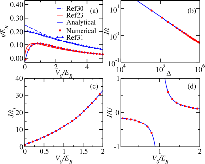
Figure 2: (Color online) (a) The exact integral of the hopping matrix $t/E_{R}$ (solid blue line) and the previous resulthopt1 ; hopt2 ; jaksch shown as function of $V_{0}/E_{R}$. Numerical integration results (red solid symbols) are also shown to check the analytical integrations. Solid triangles are data from Frankprivate . (b) $J/t$ vs $\Delta$, $\Omega_{1}=10^{5}Hz$, $\Omega_{2}=8.4\times 10^{3}Hz$, $V_{0}/E_{R}=1$. (c) $J/t_{1}$ vs $E_{R}/V_{0}$, at $\Delta=10^{5}Hz$, $\Omega_{1}=10^{5}Hz$, $\Omega_{2}=8.4\times 10^{3}Hz$. (d) $J/U$ vs $V_{0}/E_{R}$, $a_{1D}=1.27\times 10^{-12}m$, $\Omega_{1}=4\times 10^{5}Hz$, $\Omega_{2}=3.36\times 10^{4}Hz$.

The ratios between the parameters $J/t$, $J/U$, and $J/t_{1}$ can be tuned in a wide range, $0.5\textless J/t\textless 20$, $-1\textless J/U\textless 1$ and $0\textless J/t_{1}\textless 35$, and will cover the phase transition pointsqpt studied in the following sections. This will help us to observe the outcome in the optical lattice.

Figure 2 (a) shows the hopping-matrix elements by three different methods. Previous work hopt1 ; hopt2 showed the exact solution in the limit $V_{0}/E_{R}\gg 1$ from the one dimensional Mathieu equation. The result is

$$\frac{t}{E_{R}}=\frac{4}{\sqrt{\pi}}s^{\frac{3}{4}}e^{-2\sqrt{s}},$$ (5)

where the ratio is $s=\sqrt{\frac{V_{0}}{E_{R}}}$ and the coil energy is $E_{R}=\frac{\hbar^{2}k^{2}}{2m_{a}}$. In the present work, through exact symbolic integration from the Maple computer algebra systemmaple , we get the analytical expression for the hopping element $t/E_{R}$, and the analytical expression is

$$\frac{t}{E_{R}}=\frac{1}{4}(\pi^{2}s^{2}-2s^{2}-2s)e^{-\frac{\pi^{2}}{4}s}-\frac{1}{2}s^{2}e^{-\frac{1}{4}\pi^{2}s-\frac{1}{s}}$$ (6)

Figure 2(a) shows that numerical integration is consistent with the analytical results and thus both approaches are vindicated. The result of Eq. (5) becomes consistent with the analytical integration in the regime about $V_{0}/E_{R}\geq 4$.

The width of the lowest band energyjaksch is used to evaluate the hopping element $t/E_{R}$, from which we know the degree of approximation of the Gaussian Wannier function. An alternative definition of the hopping element $t/E_{R}$, which does not require the definition of Wannier states is a big advantageprivate . The hopping element is defined byprivate ; frankthesis

$$J_{exact}=\frac{1}{N}\sum_{k}E_{k}e^{ika},$$ (7)

where $N$ is the numbers of the sites, $a$ is the crystal length of the lattice, and $k$ is the wave length of the particle. This equation is also the Fourier transform of Eq. (43) of Bloch’s reviewhopt2 .

The expression of the trimer tunneling $J$ can also be obtained analytically by the $\Omega_{1}$ and $\Omega_{3}$ and $\Delta$. Here

$$\Omega_{1}=\Omega\sqrt{1/2\pi}\alpha e^{-\frac{3}{128}\alpha^{2}\lambda^{2}},$$

and

$$\Omega_{3}=\Omega\sqrt{1/2\pi}\alpha e^{-\frac{11}{128}\alpha^{2}\lambda^{2}}.$$

The ratio of $J/t$ varies from $0.5$ to $20$ as a function of $\Delta$, as shown in Fig. 2(b). Similarly, the ratio of $J/t_{1}$ is also given in Fig. 2(c).

To obtain the ratio of $J/U$, we should consider the on-site interaction $U_{0}$ as follows

$$U_{0}=g_{2}\int_{-\infty}^{+\infty}|w_{a}(x)|^{4}dx=\frac{g_{2}\alpha}{\sqrt{2\pi}},$$ (8)

where the coefficient $g_{2}$ is the coupling constant of the repulsion between two bosons and $g_{2}=\frac{2\hbar^{2}}{ma_{s}}$ in one dimensional optical lattice1dlength . The ratio $J/U$ is shown in Fig. 2(d).

III Methods and observables

To confirm the results presented in this article, we use the mean field method (MF), the self-improved Quantum Monte-carlo (QMC), and the density matrix renormalization group (DMRG) method. We compare the results from each for certain parameters.

III.1 Mean field method

The MF method is a very useful and efficient tool to deal with the quantum many body problem, though the results need to be checked by numerical methods. Here, we show how to deal with the trimer tunneling, the density dependent tunneling term and the effects of temperature in the frame of MF.

Similarly, with the decoupling approximationdec defined by:

$$a_{i}^{{\dagger}}a_{j}=\langle a_{i}^{{\dagger}}\rangle a_{j}+a_{i}^{{\dagger}}\langle a_{j}\rangle-\langle a_{i}^{{\dagger}}\rangle\langle a_{j}\rangle,$$ (9)

we get

$$a_{i}^{3{\dagger}}a_{j}^{3}=\langle a_{i}^{{\dagger}3}\rangle a_{j}^{3}+a_{i}^{{\dagger}3}\langle a_{j}^{3}\rangle-\langle a_{i}^{{\dagger}3}\rangle\langle a_{j}^{3}\rangle.$$ (10)

To simplify the equations, we let $\Psi_{a}=\langle a\rangle$, $\Psi_{t}=\langle a^{3}\rangle$ and $\rho=\langle n\rangle$.

For the density dependent terms, we decouple them in terms of:

$$n_{i}a_{i}^{\dagger 2}a_{j}^{2}=\langle n_{i}a_{i}^{\dagger 2}\rangle a_{j}^{2}+n_{i}a_{i}^{\dagger 2}\langle a_{j}^{2}\rangle-\langle n_{i}a_{i}^{\dagger 2}\rangle\langle a_{j}^{2}\rangle,$$ (11)

and

$$n_{i}^{2}a_{i}^{\dagger}a_{j}=\langle n_{i}^{2}a_{i}^{\dagger}\rangle a_{j}+n_{i}^{2}a_{i}^{\dagger}\langle a_{j}\rangle-\langle n_{i}^{2}a_{i}^{\dagger}\rangle\langle a_{j}\rangle,$$ (12)

where the variational parameters are denoted as $\Psi_{na}=\langle n_{i}^{2}a_{i}^{\dagger}\rangle$, $\Psi_{np}=\langle n_{i}a_{i}^{\dagger 2}\rangle$ and $\Psi_{p}=\langle a_{j}^{2}\rangle$ . We can deal with $a_{i}^{\dagger 2}n_{j}a_{j}^{2}$ by a similar method and we only need to pay attention to the case $\langle na^{2}\rangle\neq\langle na^{2\dagger}\rangle$. The work of Refmfde also uses the different variational order parameter for different density dependent terms.

The Hamiltonian on the total lattice can be considered as the sum over local operators on sites $i$ and $h_{i}$ and is as follows:

$$\begin{split}h_{i}=&-zt\left[(a_{i}^{{\dagger}}+a_{i})\Psi_{a}+\Psi_{a}^{2}\right]\\ &-zt_{p}\left[(a_{i}^{3{\dagger}}+a_{i}^{3})\Psi_{t}+\Psi_{t}^{2}\right]+H_{3}\end{split}$$ (13)

where we neglect the density dependent terms and $z$ is the coordination number. The stable solutions of order parameters are solved iteratively for the ground states.

To explore the temperature effectsTMF2 , we solve the partition function and the free energy, $Z=\sum_{k=1}^{n_{t}+1}e^{-\beta E_{k}}$ and $F=-\frac{1}{\beta}\ln{Z}$. For given $U$, $t$, $\mu$, and $T$, the superfluid order parameter $\Psi_{t}$, $\Psi_{a}$ can be determined by minimizing the free energy, i.e., $\frac{\partial^{2}F}{\partial\Psi_{a}\partial\Psi_{t}}\biggr{|}_{U,t,\mu,T}=0$. The gradient descent algorithm is used to find the minimum free energy. We determine the phase diagrams according to the values in Tab. 1. The compressibility $\kappa$ is an order parameter for finite temperature phase transitionskapa .

Table 1: Values of the order parameters for typical phases.

	ASF	PSF	TSF	MI	NL
$\Psi_{a}$	$\neq 0$	0	0	0	0
$\Psi_{p}$	$\neq 0$	$\neq 0$	0	0	0
$\Psi_{t}$	$\neq 0$	0	$\neq 0$	0	0
$\kappa$	$\neq 0$	$\neq 0$	$\neq 0$	0	$\neq 0$
$\rho_{s}^{a}$	$\neq 0$	0	0	0	0
$\rho_{s}^{t}$	0	0	$\neq 0$	0	0
$C_{a}$	$\neq 0$	0	0	0	0
$C_{t}$	0	0	$\neq 0$	0	0

III.2 Improved Quantum Monte-carlo method

To check the results obtained from the MF method, we simulate the model (1) using the stochastic series expansion (SSE) QMC methodsse with the directed loop updatedirecloop . The head of a directed loop carries a creation (annihilation) operator $a(a^{{\dagger}})$ in the conventional directed loop algorithm for the BH model with single particle hopping. To simulate the pair superfluid phase, the algorithm is improved by allowing the head of a directed loop to carry a pair lode ; wz2 ; psf of creation (annihilation) operators $a^{2{\dagger}}$($a^{2}$). In the present work, to make the atom trimers active, we let the loop heads carry trimer creation (annihilation) operators $a^{3{\dagger}}$($a^{3}$).

To distinguish the ASF and the TSF states, we define two types of superfluid stiffness $\rho_{s}^{\alpha}$ as the order parametersfs :

$$\rho_{s}^{\alpha}=\frac{L^{2-d}\langle W(\alpha)^{2}\rangle}{2d\beta(9J+t)}.$$ (14)

If $\alpha=t$, $W(\alpha)$ is the winding number which can be divided without remainders. If $\alpha=a$, $W(\alpha)$ is the winding number which cannot be divided without remainders.

For a TSF phase, we define the trimer superfluid order parameter $\rho_{s}^{t}>0$ and $\rho_{s}^{a}=0$. For an ASF phase, $\rho_{s}^{a}>0$ and $\rho_{s}^{t}=0$. The factor ‘$9$’ multiplying $J$ is due to the hopping of trimer atoms, or can be understood as the inverse vorticity $\nu=1/3$. An integer vorticity $\nu=1$ is found for the ASF phase, and a half vorticity is found for the PSF phase mfy2 ; fintemp . Now we get a new vorticity $\nu=1/3$ for the TSF phase. The parameters $d$ and $L$ are respectively the system dimensionality and size, and $\beta$ is the inverse temperature.

III.3 The density matrix renormalization group method

To reiterate, we also use the DMRG methoddmrg1 to study the system. Specifically, the DMRG method is used to impart the tunneling correlations $C_{a}=\sum_{r}C_{a}(r)/L$ and $C_{t}=\sum_{r}C_{t}(r)/L$, where $C_{a}(r)=\langle a_{i}^{\dagger}a_{i+r}\rangle$ and $C_{t}(r)=\langle a_{i}^{\dagger 3}a_{i+r}^{3}\rangle$. In our calculations, we impose periodic boundary conditions and restrict the filling factor to $n_{max}=3$. An infinite-size algorithm at the chain length of $L=200$ is used to ensure a maximum number of possible correlations.

IV Ground state phase diagram and Trimer superfluid

As shown in Fig. 2(c), for deep lattices, $(J,t,U)\gg t_{1(2)}$. The Hamiltonian is reduced to:

$$H=-\sum_{\langle ij\rangle}(Ja_{i}^{\dagger 3}a_{j}^{3}+ta_{i}^{\dagger}a_{j}+H.c.)+H_{3}$$ (15)

The controllability of the parameters allows us to study the quantum phase transitions between the ASF, TSF and MI phases.

IV.1 $U=0$, $t=0$ and $\mu/J\neq 0$

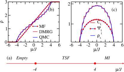
Figure 3: (Color online). The parameters are at $U=0$, $t=0$. (a) Phase diagram for the model in (15) which contains empty, TSF, and MI($\rho=3$) phases. (b) $\rho$ vs $\mu/J$ by the three methods (MF, DMRG and QMC) for the model in (15). (c) $\Psi_{t}$, $C_{t}$ and $\rho_{s}^{t}$ vs $\mu/J$.

Starting with the limit $U=0$ and $t=0$ , the TSF phase will compete with the empty phase and MI($\rho=3$) phase, as shown in Fig. 3(a). To illustrate the competition in more detail, the densities are plotted in the range of $-6<\mu/J<6$ by three different methods in Fig. 3(b). In the MF frame, we solve the matrix $h_{i}$ and then get the minimum energy in the ground state energy $E=zJ\Psi^{2}_{t}-\frac{3}{2}\mu-\frac{1}{2}\sqrt{9\mu^{2}+24z^{2}J^{2}\Psi^{2}_{t}}$. The location of the global minimum $E$ is at $|\Psi_{t}|=\frac{\sqrt{-6\mu^{2}+24z^{2}J^{2}}}{4zJ}$. Substituting the $\Psi_{t}$ into $h_{i}$, we get the exact density $\rho=\frac{3}{8}(\mu+4)$. Due to the ignorance of quantum fluctuation, the MF results is a straight line. The density from DMRG method looks like a staircase due to the finite size effects ($L=16$). QMC method gives us the same results with sufficiently lower temperature. If we increase the temperature to $\beta=2$, the data will change continuously due to finite temperature.

Now we understand the transition points between the MI and TSF phases. For the single particle picture, a trimer emerging on the empty phase will get $-6zJ$ worth of kinetic energy, but will be subjected to a cost of $-3\mu$ worth of potential energy. For the one dimensional lattice, the coordinates number is $z=2$ and consequently we get $\mu_{c}/J=\pm 4$. If we set $|\Psi_{t}|=\frac{3}{4}\sqrt{\frac{16-{\mu_{c}^{2}/J}^{2}}{6}}=0$, the transition point can be made available again.

Figure 3(c) shows the trimer superfluid stiffness in more detail. The transition points between the MI and TSF phases are consistent with those of the MF method. The maximum $\rho_{s}^{t}$ is about half of the maximum occupation number, which is similar to the case of the superfluid stiffness discussed beforemagloop . The data converges well for different sizes, so we choose $L=16$, without any loss of generality.

IV.2 $t=0$, $\mu/U\neq 0$ and $J/U\neq 0$

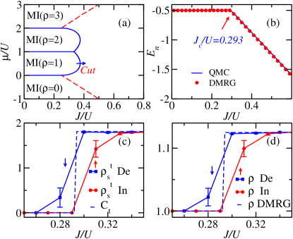
Figure 4: (Color online). (a) Phase diagram ($\mu/U$,$J/U$) of the model (15) for $t=0$. The red dashed line and blue solid line are the continuous and first order transitions, respectively. (b) Energies per site $E_{n}$ along the cut $\mu/U=0.5$ at the size $L=8$. The red circles (DMRG) and blue lines (QMC) are consistent and the phase transition point $J_{c}/U=0.293$. (c) Hysteresis loop of the $\rho_{s}^{t}$ vs $J/U$ along the cut $\mu/U=0.5$, and it is a signal of first order transition. The QMC data are obtained in a closed loop by increasing and decreasing $J/U$. (see text). $C_{t}$ is also shown to confirm the transition point. (d) Hysteresis loop of $\rho$ vs $J/U$ and $\rho$ behaviors similar to $\rho_{s}^{t}$.

Figure 4 (a) shows that, in the presence of an on-site repulsive interaction, MI($\rho=1$) and MI($\rho=2$) emerge between the TSF phases. The exact boundary of the MI-TSF phases can be derived in the MF frame. By solving the Hamiltonian matrix, four energy eigenvalues are obtained. The lowest one for $0<\mu<1$ is:

$$E=zJ\Psi^{2}_{t}-\frac{3}{2}(\mu-U)-\frac{1}{2}\sqrt{9(\mu-U)^{2}+24z^{2}J^{2}\Psi^{2}_{t}}~{}.$$

Letting $\frac{\partial E}{\partial\Psi_{t}}=0$, the superfluid order parameter is $|\Psi_{t}|=\frac{\sqrt{6}}{2}\sqrt{1-\frac{(\mu-U)^{2}}{4z^{2}J^{2}}}$, for $1-\frac{(\mu-U)^{2}}{4z^{2}J^{2}}\geq 0$. By substituting $|\Psi_{t}|$ into the energy expression, we get:

$$E_{3}=\frac{3(\mu-U)^{2}}{8zJ}-\frac{3}{2}(\mu-U)-\frac{3}{2zJ}~{}.$$

Along the boundaries of the MI-TSF phases, the energy of both phases should be equal ($E_{3}=-\mu$). The boundary is obtained as $J=\frac{3U-\mu}{12}+\frac{\sqrt{3\mu U-2\mu^{2}}}{6}$. For example, if $\mu/U=0$, then $J/U=0.25$, which is consistent with the previous expression for $J/U$.

To confirm and check the MF phase diagram, the energies are plotted along the cut $\mu/U=0.5$ by both DMRG and QMC methods and the results are consistent again. We find the energy makes a corner at $J_{c}/U=0.293$, smaller than the MF phase transition point at $J_{c}/U=0.375$, which is in the range shown in Fig. 2(c).

Figure 4(c) and (d) show two hysteresis loops for superfluid stiffness and density, which are the signals of first order transitions. In previous workmagloop , one of us found a multi-hysteric loop phenomena and located the phase transition point successfully, by increasing and decreasing the parameters in a cycle. In the present work, we use the same method. Firstly, we obtain the physical quantities $\rho$ and $\rho_{s}^{t}$, by increasing the variable $J/U$. When we decrease $J/U$, a closed loop takes form, as shown in Fig. 4(c) and (d). In the simulation, we store the last configuration, and then input it as the next initial configuration. We find that the closed loops of $\rho$ and $\rho_{s}^{t}$ behavior in a similar fashion. The correlation $C_{t}$ is also consistent with $\rho_{s}^{t}$.

IV.3 $J/t\neq 0$, $\mu/t\neq 0$ and $U=0$

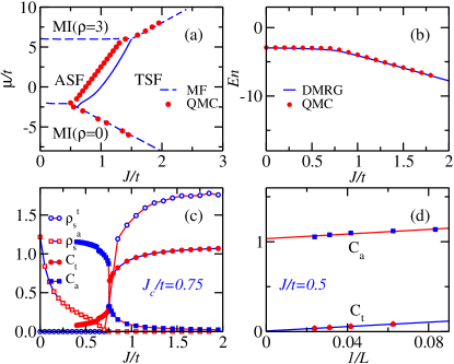
Figure 5: (Color online). (a) Phase diagram $(J/t,\mu/t)$ of the model (15) for $U=0$. The blue dashed lines and blue solid line are the continuous and first order transitions, respectively. The red solid circles are the QMC results. (b) Energy per site $E_{n}$ vs $J/t$ by DMRG and QMC methods along the cut $\mu/t=0$ at the size $L=24$. (c) $C_{t}$, $C_{a}$, $\rho_{s}^{a}$ and $\rho_{s}^{t}$ vs $J/t$. (d) The finite size scalings of $C_{t}$, $C_{a}$ in the ASF phase at $J/t=0.5$.

With both $J$ and $t$ are nonzero, it is difficult to get the analytical boundary lines. Here we provide the numerical results. Figure 5(a) shows the phase diagram in the plane $(J/t,\mu/t)$, containing the ASF, TSF and MI phases. The system exhibits an ASF phase for small $J/t$, a TSF phase for larger $J/t$, an empty phase for small $\mu/t$ and a MI($\rho=3$) for larger $\mu/t$. The ASF-TSF phase transition is clearly first order. With $J=0$, the systems undergo a MI($\rho=0$) to ASF phase transition at $\mu/t=-2$ and a MI $(\rho=3)$ to the ASF phase transition at $\mu/t=6$, which can be understood by a single particle picture.

Figure 5(b) compares the energies per site $E_{n}$ along the cut $\mu/t=0$. The energies from the different methods are well consistent with each other. They keep a constant in the ASF phase for $J/t<0.75$ and then go down in a straight line for $J/t>0.75$.

To illustrate the ASF-TSF phase transition in more detail. We shows $C_{t}$, $C_{a}$, $\rho_{s}^{a}$ and $\rho_{s}^{t}$ vs $J/t$. In the range $0<J/t<0.75$, we find $\rho_{s}^{a}$ decreases as $J/t$ increases, and $\rho_{s}^{a}$ tends to zero continuously at the phase transition point $J_{c}/t=0.75$. $\rho_{s}^{t}$ jumps to nonzero values at the same location as $\rho_{s}^{a}$ changes. These phenomenon clearly proves that the ASF-TSF phase transition is indeed of first order instead of a weak first order transitionwz1 ; wz2 . In the whole range, we also see the sharp jumps of $C_{t}$ and $C_{a}$ as $J/t$ increases. In the ASF phase, $C_{t}=0$ while $C_{a}\neq 0$ in the thermal dynamical limit, as shown in Fig. 5(d). In the TSF phase, $C_{t}\neq 0$ while $C_{a}=0$, which is not shown.

IV.4 Winding numbers and Correlation

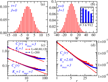
Figure 6: Histograms of the winding numbers $W$ for (a) $t=1$ is the only nonzero parameter and $W$ varies in units of unity. (b) $J=1$ is the only nonzero parameter and $W$ occurs as $0,\pm 3,\pm 6,\pm 9,...$. (c) The power law decay of the $C_{t}(r)$ in the TSF phase with $n_{max}=3$, and the $C_{a}(r)$ in the ASF phase with $n_{max}=1$. $K_{a(t)}=1$. (d) The power law decay of the correlation $C_{a}(r)$ for the softcore bosons. $K_{a}=2.68$.

In Figs. 6 (a) and (b) , we give a typical winding number distribution in the ASF and TSF phase. Clearly, both of them are represented by a Gaussian distribution. For the ASF phase, we set $t=1$ and all the other parameters are zero. The winding numbers vary in units of one, such as $0$, $\pm 1$, $\pm 2$, $\cdots$. However, for the TSF phase, we set $J=1$ and all the other parameters are zero. The winding numbers only occur as numbers which can be divided by $3$ without any remainders, such as $0$, $\pm 3$, $\pm 6$, $\cdots$. This can be understood as three atoms are bound together tightly and move in space simultaneously.

To find the relationship between the ASF phase and the TSF phase, in addition to the distribution of winding numbers, we also show the correlation between trimers and holes. We let the size of the system be as large as possible i.e. $L=60$, $80$, $120$, and $200$.

In Fig. 6(c), we plot the trimer correlation $C_{t}(r)$, and the correlation satisfies the power law decay:

$$C_{t}(r)=a_{t}^{0}r^{-\frac{K_{t}}{2}}$$ (16)

where the fitted result is $K_{t}=1$. For the ASF phase in hardcore bosons (the on-site maximum number is $n_{max}=1$), the correlation satisfies:

$$C_{a}(r)=a_{a}^{0}r^{-\frac{K_{a}}{2}},$$ (17)

where the fitted exponent is also $K_{a}=1$. The two types of correlation decay with a same exponent. This is because the TSF state can be mapped to the ASF state, if we consider the trimer as a whole molecule. At the same time, the above two cases are non-interactive systemscolex . However, if $n_{max}=3$, then $K_{a}=2.68$ which is larger than $K_{a}=1$, as shown in Fig. 6(d). In this case, the atom tunneling will be hindered by the additional bosons. Then the correlation will decay more quickly than the cases for $K_{a(t)}=1$.

V Effects of density dependent tunneling

Besides the atom hopping and trimer hopping terms, the occupation dependent terms with $H_{n1}=-t_{1}\left(n_{i}^{2}+n_{j}^{2}\right)a_{i}^{\dagger}a_{j}$ and $H_{n2}=-t_{2}\left(n_{i}+n_{j}\right)a_{i}^{\dagger 2}a_{j}^{2}$ , are easily overlooked, as they are smaller than $J$ and $t$ in a wide range of parameters. Refxfzhou ; ddt1 ; ddt2 only mentioned the similar terms without the detailed discussion of the effects of $H_{n1}$ and $H_{n2}$ to the ASF-TSF phase transition. However, $t_{1}$ and $t_{2}$ are coupled with density operators, which will change the phase diagram sufficiently. So it is necessary to explore the competition between $t_{1}(t_{2})$, $J$ and $\mu$. However, experimentally, as discussed in Sec. II, the parameter $t_{1}$ equals $t_{2}$ and cannot be tuned independently and consequently we define $t_{12}=(t_{1}+t_{2})/2$ to study the physical consequences of having both $t_{1}$ and $t_{2}$ being nonzero.

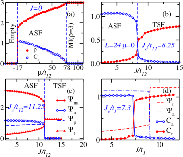
Figure 7: (Color online) (a) $\rho$ (solid circles) and $C_{a}$ (empty circles) vs $\mu/t_{12}$ with $J=0$. The phase transition point is $\mu_{c}/t_{12}=-17$ between the empty phase and the ASF phase. (b) $C_{t}$ and $C_{a}$ vs $J/t_{12}$ with $\mu=0$. The ASF-TSF phase transition point is at $8.25$ by the DMRG method. (c) MF results of quantities $\Psi_{p}$, $\Psi_{a}$, $\Psi_{na}$ and $\Psi_{t}$ as function of $J/t_{12}$. The MF phase transition point is at $J/t_{12}=11.25$. (d) MF and DMRG results of quantities $C_{t}$, $C_{a}$, $\Psi_{a}$ and $\Psi_{t}$ as functions of $J/t_{1}$.

Figure 7 (a) shows $\rho$ vs $\mu/t_{12}$ at $J=0$. The jump in the densities and the correlation $C_{a}$ confirm that the empty -ASF phase transition is first order. However, the empty phase to ASF phase transition is continuous for the BH model with $t_{12}=0$. The accurate phase transition point is available and is at $\mu_{c}/t_{12}=-17$. The single particle picture fails to analyze the empty-ASF phase transition points. Due to the presence of the term like $a_{i}^{+}n_{j}^{2}a_{j}$, the system needs at least two atoms emerging on the site $j$ from the empty to the ASF phase.

Furthermore, by turning on $J$, we show the density dependent tunneling $t_{12}$ effect to the quantum phase transition at $\mu=0$ in Fig. 7 (b). Compared with $J_{c}/t=1$ in Fig. 5 (a), the phase transition point is $J/t_{12}=8.25$, sufficiently modified by the coupled density operators. In the presence of the finite size effect, $C_{a}\neq 0$ in the TSF phase. However, we find $C_{a}=0$ and $C_{t}\neq 0$ in the thermal dynamical limit, which is not shown.

Figure 7 (c) shows the MF results of quantities $\Psi_{p}$, $\Psi_{a}$, $\Psi_{na}$, and $\Psi_{t}$ as function of $J/t_{12}$. In the ASF phase, all of the quantities are nonzero while only $\Psi_{t}$ is nonzero in the TSF phase. To check which term causes the first-order ASF-TSF phase transition by $J/t_{12}$, we set $t_{2}=0$ and only show effects of $J/t_{1}$ in Fig. 7 (d). The phase transition point is at $J/t_{1}=7.3$ and also sufficiently modified by the coupled density operators. The MF results are also given, in similar fashion to the case of $J/t_{12}$.

VI Finite temperature effects

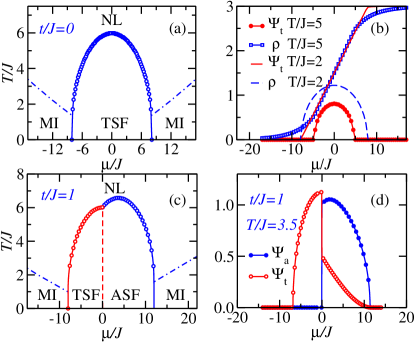
Figure 8: (Color online) $U=0$ and $t=0$ (a) Finite temperature MF phase diagram ($\mu/J$, $T/J$), which contains MI, TSF, NL phase for $U=0$ and $t=0$. (b) $\Psi_{t}$ and $\rho$ vs $\mu/J$ for $T/J=2$ and $T/J=5$. (c) The finite temperature MF phase diagram ($\mu/J$,$T/J$). (d) $\Psi_{t}$ and $\Psi_{a}$ for $T/J=3.5$.

Since there is no thermal Berezinskii-Kosterlitz-Thouless(BKT) phase transition for the 1-D classical or quantum system, we choose a two dimensional systemkt as a candidate to study the thermal melting of the TSF.

The phase diagram in both the MF frame are drawn. In Fig. 8 (a), on both sides, the MI-normal liquid(NL) boundary lines are linear. As shown in previous workkapa , $\kappa=0$ in the MI phase. Since there is no long range order for both the MI and NL phases, the value $\kappa$ updates without any singularity into a nonzero value in the NL phase at finite temperature. Therefore, we use the criterion $\kappa=0.002$ to obtain the MI-NL crossover boundary lines.

The TSF phases emerges in a leaf shaped region, for lower temperatures, in the range of $-8<\mu/J<8$. The boundaries between MI-TSF phases are consistent with the analysis in the zero temperature limit. The transition temperatures of the TSF-NL phases varies with different chemical potentials. At $\mu=0$, the TSF-NL transition point is $T/J=6$. In Fig. 8(b), we plot density $\rho$ and correlation $\psi_{t}$ as function of $\mu/J$ with different temperatures $T/J=2$ and $T/J=5$.

Figure 8(c) shows the finite temperature phase diagram, where both $t$ and $J$ are nonzero. We find MI,TSF, ASF phases at lower temperatures, and NL phase for higher temperatures. There is no obvious difference between the boundary lines of TSF-NL and the ASF-NL phases. Therefore, the cold-atom experiment can observe the TSF phase in the temperatures just as the ASF phase. In Fig. 8(d), we describe $\Psi_{t}$ and $\Psi_{a}$ in more detail. At $T/J=3.5$, we scan $\mu/J$, and find the TSF phase in the range $-6.8<\mu/J<0$ and the ASF phase in the range $0<\mu/J<11.6$ . The jump of the order parameters $\Psi_{t}$ and $\Psi_{a}$ clearly demonstrates that the phase transition between ASF-TSF phases is of first order, even at finite temperatures.

VII Discussion and conclusion

The ASF phase is of type $\langle a\rangle\neq 0$, $\langle a^{3}\rangle\neq 0$ and $Z_{2}$ broken symmetry, while the TSF phase is of type $\langle a^{3}\rangle\neq 0$ and $U(1)$ broken symmetrysym . According to the Landau-Ginzburg-Wilson paradigm, different broken symmetry patterns make the ASF-TSF quantum phase transition first order. On the other hand, the $Z_{2}$ broken symmetry corresponds to an Ising phase transition. However, by the Coleman-Weinberg mechanismmecha and our calculation, the ASF-TSF phase transition becomes a first-order one driven by the large quantum fluctuation.

At finite temperatures, we choose a two-dimensional lattice as a platform to study the temperature effects. We provided the MF results of the transition points of the thermal melting of the TSF phase. By the MF method, the ASF-TSF phase transition is first order at $T>0$. Further careful checking is needed by other methods.

In conclusion, we derived a new BH model with trimer tunneling and two types of density dependent tunneling. We improved the QMC algorithm for simulation of trimer tunneling. We studied the ground state quantum phase diagram in a one-dimensional lattice by three different methods, which agree with each other in applicable regimes. The parameters to be realized were also discussed, and various interesting phase transitions were studied. We found the first-order empty-ASF phase phase transition in the presence of the density dependent tunneling terms. Our results will be helpful in guiding the optical experimentalists to realize the trimer superfluid.

Appendix A The hopping $t/E_{R}$ for the deep well

Figure 2 (a) shows the atom tunneling amplitude $t$, both numerically and analytically, which is defined by

$$t=-\int_{-\infty}^{+\infty}w_{a}(x-x_{i})H(x)w_{a}^{*}(x-x_{j})dx,$$ (18)

where $H(x)=(\frac{-\hbar^{2}}{2m}\frac{d^{2}}{dx^{2}}+V(x))$ is the Hamiltonian of the system. Here the optical potential is $V(x)=V_{0}sin^{2}(kx)$, where the wave number $k=2\pi/\lambda$, $\lambda=500nm$. The Wannier functions of an atom (or molecule) are of Gaussian type:

$$w_{a(m)}(x)=\left[\alpha^{2}/\pi\right]^{\frac{1}{4}}e^{-\frac{\alpha^{2}x^{2}}{2}},$$ (19)

and the characteristic lengthopticallattice is :

$$\alpha^{-1}=\left(\hbar^{2}2m_{a(m)}V_{0}/k^{2}\right)^{1/4}.$$ (20)

Previous work hopt1 ; hopt2 showed the exact solution in the limit $V_{0}/E_{R}\gg 1$ from the one dimensional Mathieu equation. In the present work, through exact symbolic integration from the Maple computer algebra systemmaple , we get the analytical expression for the hopping matrix element:

$$\frac{t}{E_{R}}=\frac{1}{4}(\pi^{2}s^{2}-2s^{2}-2s)e^{-\frac{\pi^{2}}{4}s}-\frac{1}{2}s^{2}e^{-\frac{1}{4}\pi^{2}s-\frac{1}{s}}$$ (21)

for the ratio $s=\sqrt{\frac{V_{0}}{E_{R}}}$ and the coil energy $E_{R}=\frac{\hbar^{2}k^{2}}{2m_{a}}$. Note that in this integral, we set $x_{i}=-\lambda/4$ and $x_{j}=\lambda/4$. The solution is also based on the approximated Wannier function.

Appendix B The hopping $t/E_{R}$ for the wells with any depth

According to Frank Deuretzbacherprivate , Eq. (7) can be simplified to:

$$J_{exact}=-\int_{0}^{1}E_{\kappa}\cos(\pi\kappa)d\kappa,$$ (22)

where $\kappa=\frac{ka}{\pi}$. $E_{\kappa}$ can be obtained by solving the one-dimensional Mathieu function, and the expression is

$$\frac{E_{k}}{E_{R}}=a(\kappa,-\frac{V_{0}}{4E_{R}})-\frac{V_{0}}{2E_{R}}.$$ (23)

In the equation above, the function “a” is the MathieuCharacteristicA function in Mathematica or MathieuA in Maple. Substituting Eq. (23) into Eq. (22), the numerical result is available as shown in Fig. 2(a).

This result is simply the outcome of having the Hamiltonian operate on the eigenfunction, getting the eigenvalue “a” and the simply integrating over the product of Mathieu functions which yields unity because they are normalized. To reiterate, the Mathieu “a” function is, apart from an offset, the energy of a Bloch state (Eq. (23)). So, inserting it into Eq. (18), the usual definition of $J$, the formula that connects the Wannier functions to the Bloch functions (i.e. the discrete Fourier transform of the Bloch functions), then using the fact that the Mathieu “a” functions are the eigenenergies of the Bloch functions, and from the orthogonality and the normalization of the Bloch functions, Eq. (7) is finally obtained.