Characterization of quantum dynamics using quantum error correction

Abstract

Characterizing noisy quantum processes is important to quantum computation and communication (QCC), since quantum systems are generally open. To date, all methods of characterization of quantum dynamics (CQD), typically implemented by quantum process tomography, are off-line, i.e., QCC and CQD are not concurrent, as they require distinct state preparations. Here we introduce a method, “quantum error correction based characterization of dynamics”, in which the initial state is any element from the code space of a quantum error correcting code that can protect the state from arbitrary errors acting on the subsystem subjected to the unknown dynamics. The statistics of stabilizer measurements, with possible unitary pre-processing operations, are used to characterize the noise, while the observed syndrome can be used to correct the noisy state. Our method requires at most $2(4^{n}-1)$ configurations to characterize arbitrary noise acting on $n$ qubits.

I Introduction

The principal difficulty in implementing quantum computation physically is environment-induced noise, which decoheres the quantum system, resulting in the loss of superposition and of entanglement. The noise acting on a quantum system starting initially in a product state with its environment is described by a completely positive (CP) map and is represented by the Kraus operators Nielsen and Chuang (2000) $E_{j}\equiv\sum_{i}\alpha_{i,j}F_{i}$, where $F_{i}$ is an element from an operator (or error) basis satisfying the orthogonality condition Tr$(F_{i}F^{\dagger}_{j})=d\delta_{i,j}$, where $\delta_{i,j}$ is the Kronecker delta, and $d=2^{p}$ is the dimension of the system, consisting of $p$ qubits. Thus, if $\rho$ represents the initial quantum state, then

$$\mathcal{E}(\rho) = \sum_{j}E_{j}\rho E^{\dagger}_{j}=\sum_{m,n}\chi_{m,n}F_{m}\rho F_{n}^{\dagger}$$ (1)

where $\chi_{m,n}\equiv\sum_{j}\alpha_{j,m}\alpha^{\ast}_{j,n}$ is a Hermitian matrix (the “process matrix”) in the $d^{2}$-dimensional Hilbert-Schmidt space of linear operators acting on the system of dimension $d$. From the completeness condition, we have $\sum_{j=1}^{d^{2}}E_{j}^{\dagger}E_{j}=\sum_{m,n}\chi_{m,n}F^{\dagger}_{m}F_{n}=\mathbb{I}$, which imposes $d^{2}$ conditions, so that the matrix $\chi$ has $d^{4}-d^{2}$ independent real elements. Since taking trace on both sides yields $\sum_{j}\chi_{j,j}=1$, the (positive) diagonal elements of $\chi$ can be interpreted as probabilities. In this work, $F_{j}$ are multi-qubit Pauli operators, which is appropriate for employing the QEC formalism.

The characterization of noisy quantum processes, namely determining the matrix elements $\chi_{m,n}$, was initially addresed by standard quantum process tomography (SQPT) Nielsen and Chuang (2000); D’Ariano (2000). Here the system undergoing the unknown noisy dynamics is initially prepared in suitable states and subjected to state tomography measurements. In ancilla-assisted process tomography (AAPT) Altepeter et al. (2003), the principal system P and an ancillary system A are prepared in suitable initial states, and information about the dynamics of P is extracted via quantum state tomography on the joint system using separable or non-separable basis measurements. SQPT and AAPT are indirect in that they first obtain full state tomographic data $\mu_{m,n}=\textrm{Tr}(\rho_{m}\mathcal{E}(\rho_{n}))$ on input states $\rho_{n}$, and then invert this exponentially large data (of size $d^{4}-1$ in SQPT and $d^{4}-d^{2}$ in AAPT under trace-preserving noise) to derive $\chi$.

By contrast, direct characterization of quantum dynamics (DCQD) Mohseni and Lidar (2006, 2007), bypasses the state tomography. It uses quantum error detection measurements augmented by normalizer measurements in a code-space determined by stabilizers corresponding to Bell-state measurements. Other recent developments include the characterization of noise using an efficient method for transforming a channel into a symmetrized (i.e., having only diagonal elements in the process matrix) channel via twirling Emerson et al. (2007), suitable for identifying quantum error correcting codes (QECCs) Silva et al. (2008). Recently, three independent proposals have been presented to rapidly estimate the channel using quantum error correction (QEC) techniques Fowler et al. ; Combes et al. ; Fujiwara , which aim for concurrent preservation of quantum information, rather than for process tomography of the dynamics of P. A method similar to Emerson et al. (2007), but extended to efficiently estimate any given off-diagonal term, was introduced in Ref. Bendersky et al. (2008).

Suppose we have a situation where it is known with reasonable confidence that an arbitrary noise is restricted to a certain known, sufficiently small subsystem of a quantum computation and communication (QCC) device, say a quantum computer. One can construct QECCs that would protect against the noise. On the other hand, the statistics of the measured syndrome outcomes could be used for characterization of that noise, which could be useful for other quantum information processing tasks. A method that helps combine QCC and characterization of quantum dynamics (CQD) would thus surely help save valuable quantum resources. In this work, we present such a method, a QEC-based characterization of quantum dynamics (QECCD). The reason that the noise must be restricted to a known subsystem of the quantum computer is that the allowed errors must form a group, for a reason that will become clear later. Without the subsystem restriction, our method can still be used to determine the diagonal terms of the process matrix in the Pauli representation.

From the perspective of CQD, our method allows initial states that are not fixed but, instead, can be any thing in the code space of a QECC. This means that the noise characterization is indifferent to certain kinds of errors in state preparation, namely those that keep the state within the stabilized code space. Our method is presently restricted to CP–but not necessarily trace-preserving–maps, though the QEC formalism is known Shabani and Lidar (2009) to be applicable even to non-CP maps.

The remainder of this work is as follows. Section II presents the basic motivation for using QECC for CQD. The basic intuition here is an isomorphism that can be established between the allowed noise and the erroneous version of the logical state. In Section II.1, we introduce a different type of stabilizer codes that are suitable for CQD. These are QECCs that correct all possible errors that occur on known coordinates and form a group. Here we give an example of a five-qubit QECC that corrects all errors on the first two qubits, and furthermore is perfect (i.e., it saturates the quantum Hamming bound). In Sec. II.2, we show how the statistics of syndrome outcome data on this kind of QECCs can be used to read off the diagonal terms of the process matrix. Accessing off-diagonal terms is a bit more involved. In principle, a suitable unitary can be used to rotate off-diagonal terms in such a way that a syndrome measurement can access them. We show how this is done in Sec. II.3. However, this method can only access the real or imaginary part of off-diagonal terms. In Sec. II.4, we show how a “toggling” can be customized to the above unitary, such that the real and imaginary parts of the accessed off-diagonal terms can be ‘toggled’, i.e., exchanged, so that after toggling, the method of Sec. II.3 can be used. In Sec. III, we consider experimental aspects. We point out that various QECCD experiments are well within the reach of an experimental facility (NMR, quantum optics, etc.) where entanglement generation and manipulation are done. An example of QECCD of a single-qubit noise, that would be suitable for experimental implementation, is worked out in detail. To this end, we introduce a new three-qubit perfect stabilizer code, which is applied to an amplitude damping channel on the first qubit. Finally, we conclude in Sec. IV.

II Noise characterization and QECCs

Like DCQD, our method is direct and requires initial entangled states. However, unlike DCQD and other quantum process topography (QPT) methods, QECCD requires no special initial state preparation: any state in the $2^{k}$-dimensional code space of an $[[n,k]]$ $n$-qubit stabilizer code for QEC is appropriate, provided the code corrects arbitrary errors on $m$ $(<n)$ known coordinates of P. The syndrome obtained from the stabilizer measurement can be used to correct the noisy state, while the experimental probabilities of syndromes will contain information about the noise channel.

We recollect that the code is a subspace $\mathcal{C}$, whose projector $\Pi_{\mathcal{C}}$ satisfies the error correcting condition $\Pi_{\mathcal{C}}F^{\dagger}_{a}F_{b}\Pi_{\mathcal{C}}=C_{ab}\Pi_{\mathcal{C}}$, where $C_{ab}$ is a Hermitian matrix Gottesman . In the case of non-degenerate QECCs (where $C_{ab}$ is non-singular), this defines a bijective mapping between the allowed noise channel and states in the error ball about any QECC-encoded state $|\Psi_{L}\rangle$, akin to a Choi-Jamiolkowski isomorphism Omkar et al. (2013). This follows from the one-to-one correspondences:

$$\mathcal{E}\longleftrightarrow\{\chi_{m,n}\}\longleftrightarrow\sum_{m,n}\chi_{m,n}|\Psi_{L}^{m}\rangle\langle\Psi_{L}^{n}|,$$ (2)

where the first correspondence follows by definition, and the second from the fact that $\{|\Psi^{m}_{L}\rangle\equiv F_{m}|\Psi_{L}\rangle\}$ forms a basis in the error ball about $|\Psi_{L}\rangle$. QECCD can be seen as exploiting the QECC isomorphism to determine matrix $\chi$ in that various measurements on $\mathcal{E}(|\Psi_{L}\rangle\langle\Psi_{L}|)$, the noisy version of the initial logical state $|\Psi_{L}\rangle$, will suffice to extract all information about $\mathcal{E}$, while extracting no information about the encoded state $|\Psi\rangle$. This result is non-trivial, since such an isomorphism exists quite generally for arbitrary QECCs, but the experimental accessibility of off-diagonal terms of the process matrix in the Pauli representation is possible in this approach only when the allowed errors form a group. Thus a general QECC cannot necessarily serve QECCD.

The scheme for QECCD is depicted in Fig. 1. Some of the qubits will be allowed to be noisy and others are assumed to be clean. The former qubits constistute the principal system P; the latter the CQD ancilla A.

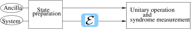
Figure 1: (Color online) Scheme for QECCD: The principal system P (subjected to the uncharacterized noise $\mathcal{E}$) plus CQD ancilla A (assumed to be noiseless) are prepared in a QECC-encoded state. After P is subjected to channel $\mathcal{E}$ (assumed correctable by the QECC used), the stabilizers are measured on the joint system, possibly following unitary operation $U$ or $US^{+}$.

Suppose the full system $\textbf{P}+\textbf{A}$ is in the state $|\Psi_{L}\rangle\equiv\sum_{j=0}^{2^{k}-1}\beta_{j}|j_{L}\rangle$, where $\{|j_{L}\rangle\}$ denotes a logical basis for the code space of a $[[p+q,k]]$ QECC (which encodes $k$ qubits into $n\equiv p+q$ qubits) such that allowed errors in the $p$ known coordinates of P can be detected and corrected. An assumption here is that no (appreciable) errors occur on the $q$ ancillary qubits. The stabilizers $S_{j}$ are a set of $p+q-k$ mutually commuting binary $n$-qubit observables that stabilize the code space (i.e., $S_{j}|j_{L}\rangle=|j_{L}\rangle$). Correctable errors $F_{i}$ are such that for any pair $F_{i},F_{j}$ ($i\neq j$), there is at least one $S_{i}$ that anti-commutes with the product $F_{i}F_{j}$. This ensures that the eigenvalue pattern for each correctable error, which is the error syndrome, is distinct. The Hamming bound Gottesman in this case is given by $2^{k}V\leq 2^{p+q}$, where $V$ is the size of the error ball, here the set of all possible errors in P, so that $V=\sum_{r=0}^{p}{p\choose r}3^{r}\cdot 1^{p-r}=4^{p}=d^{2}$ (since $d=2^{p}$). The Hamming bound for QECCD is thus $q\geq k+p$.

II.1 A class of stabilizer codes suitable for CQD

To see the connection between QEC and CQD, consider the $[[5,1]]$ code that saturates the Hamming bound for an arbitrary single-qubit error on any qubit:

$$|0_{L}\rangle = \frac{1}{2\sqrt{2}}(|00000\rangle+|00110\rangle+|01001\rangle-|01111\rangle$$

$$~{}~{}~{}-|10011\rangle+|10101\rangle+|11010\rangle+|11100\rangle)$$

$$|1_{L}\rangle = XXXXX|0_{L}\rangle,$$ (3)

where the states are represented in the computational basis, and $X$ is the Pauli-$X$ operator. We note that the above code words satisfy the error correcting conditions when the allowed errors are arbitrary errors on the first two qubits. Thus, let the first two qubits constitute P, subjected to unknown dynamics, while the remaining three are CQD ancillas. There are 16 basis elements for the general noise acting on these two qubits, represented by $X^{\bf u}Z^{\bf v}$, where ${\bf u}=(u_{1},u_{2})$ and ${\bf v}=(v_{1},v_{2})$ are vectors defined over $GF(2)$.

The stabilizer generators

$$\mathcal{G}\equiv\{IZZZZ,XXXII,ZXZIX,ZZXXI\}$$ (4)

uniquely determine the four syndromes to be $(u_{2},v_{1}\oplus v_{2},u_{1}\oplus v_{2},u_{1}\oplus u_{2})$. It is worth stressing that code (3) is different from that in Ref. Laflamme et al. (1996) because the stabilizers, and thus the set of correctable errors, are different, even though the code words are the same. The main point for QECCD is that the set $\mathbb{E}$ of correctable errors (up to scalar factors $\pm 1$ and $\pm i$), form a group, the error group. This is reflected in the above Hamming bound for QECCD. Suppose the unknown dynamics is a (correlated) noise given by the Kraus operators $\{\sqrt{1-p}I,\sqrt{p}X_{1}X_{2}\}$. From Eq. (1) one finds that the probability that no error happens, and thus that to experimentally find the no-error syndrome $(1,1,1,1)$, is $\chi_{I,I}=1-p$. Similarly, the syndrome $({-1},1,{-1},1)$ for error $X_{1}X_{2}$ occurs with probability $\chi_{X_{1}X_{2},X_{1}X_{2}}=p$. The syndrome carries information only about the noise, and nothing about the encoded state, and can be used to correct the noisy version of $|\Psi_{L}\rangle$, while the error statistics determined by the syndrome outcomes helps determine the elements of matrix $\chi$. (There are no off-diagonal terms of $\chi$ for this channel in the Pauli operator representation.)

Now consider a variant of the above example, wherein we consider letting P be all 5 qubits, while the noise is taken to be an arbitrary one-qubit error on any one qubit. This is just the five-qubit code of Ref. Laflamme et al. (1996). Though the above five-qubit QECC is suitable for QEC here, still the correctable errors do not form a closed set and, thus, do not constitute an error group: e.g., while $X_{1}$ and $Y_{2}$ can be corrected, their product $X_{1}Y_{2}$ cannot. Although the diagonal terms of the process matrix can still be calculated, for the off-diagonal terms, our method requires this closure property.

II.2 Determining the diagonal terms of $\chi_{m,n}$

Given $\mathcal{E}$ known to be correctable by a non-degenerate QECC $Q$, but otherwise uncharacterized, a single configuration suffices to determine all diagonal elements $\chi_{m,m}$ via measurement of the (mutually commuting) stabilizers of $Q$. We refer to the corresponding observable as the syndrome operator, $\Sigma$. The measurement of syndrome $x$, corresponding to error $F_{x}$, collapses the noisy state into the pure state $F_{x}|\Psi_{L}\rangle$, which can be corrected by applying $F^{\dagger}_{x}=F_{x}$. The probability of obtaining outcome $x$ is:

$$\xi(x)=\textrm{Tr}\left(\mathcal{E}\left(|\Psi_{L}\rangle\langle\Psi_{L}|\right)\left[\sum_{J=0}^{2^{k}-1}|J^{x}\rangle\langle J^{x}|\right]\right)$$

$$=\langle\Psi_{L}^{x}|\left[\sum_{m,n}^{d^{2}-1}\chi_{m,n}|\Psi_{L}^{m}\rangle\langle\Psi_{L}^{n}|\right]|\Psi_{L}^{x}\rangle$$

$$=\sum_{m,n=0}^{d^{2}-1}\chi_{m,n}\delta_{x,m}\delta_{x,n}=\chi_{x,x},$$ (5)

where it is convenient to take the tracing basis to be any completion of $\{F_{j}|\Psi_{L}\rangle\}$.

II.3 Determining the off-diagonal terms of $\chi_{m,n}$

Off-diagonal terms are obtained by pre-processing the noisy state using a unitary $U$ or $US^{+}$, prior to stabilizer measurement. [Equivalently, measurements are made in one of two bases: the “rotated basis” $U\Sigma U^{\dagger}$ or the “toggled and rotated basis” $(US^{+})\Sigma(US^{+})^{\dagger}$, as explained below.] Here again, the state just after measurement will be $F_{x}|\Psi_{L}\rangle$, for some correctable $F_{x}$. Consider a unitary operator $U(a,b)=\frac{F_{a}+F_{b}}{\sqrt{2}}$, where allowed errors $F_{a}$ and $F_{b}$ anti-commute (else, we choose $U=\frac{F_{a}+iF_{b}}{\sqrt{2}})$, such that $F_{a}F_{x}$ and $F_{b}F_{x}$ represent correctable errors. This is guaranteed by choosing a QECC whose correctable Pauli errors form a group (up to a scalar factor $\pm 1$ or $\pm i$) under multiplication. This requirement is met, as in the first example above, by choosing a QECC that corrects arbitrary errors on subsystem P. Let $g_{A}F_{A}\equiv F_{a}F_{x}$, where $F_{A}$ is a Pauli operator and the Pauli factor $g_{A}\in\{\pm 1,\pm i\}$. Similarly, let $g_{B}F_{B}\equiv F_{b}F_{x}$. For example, if $F_{a}=X,F_{x}=Y$, then $F_{A}=Z$ and $g_{A}=+i$. If $g_{A}$ and $g_{B}$ are both real or both imaginary, then we say that the Pauli factors are of the same type. If one of $g_{A}$ and $g_{B}$ is imaginary and the other real, we say that the Pauli factors are of distinct type.

Operation $U(a,b)$ rotates one correctable state to another correctable state. This alters the statistics of the stabilizer measurement without affecting the correctability. The probability of finding the syndrome corresponding to error $F_{x}$ is now:

$$\xi(a,b,x)\equiv$$

$$\textrm{Tr}\left(U(a,b)\mathcal{E}\left(|\Psi_{L}\rangle\langle\Psi_{L}|\right)(U(a,b))^{\dagger}\left[\sum_{J=0}^{2^{k}-1}F_{x}|J\rangle\langle J|F_{x}\right]\right)$$

$$=\frac{\sum_{m,n}^{d^{2}-1}\chi_{m,n}\langle F_{x}\left(F_{a\star m}+F_{b\star m}\right)\rangle_{L}\langle\left(F_{n\star a}+F_{n\star b}\right)F_{x}\rangle_{L}}{2}$$

$$=\frac{1}{2}\sum_{m,n}^{d^{2}-1}\chi_{m,n}\left(g^{\ast}_{A}\delta_{A,m}+g_{B}^{\ast}\delta_{B,m}\right)\left(g_{A}\delta_{A,n}+g_{B}\delta_{B,n}\right)$$

$$=\frac{\chi_{A,A}+\chi_{B,B}}{2}+\frac{g_{A}^{\ast}g_{B}\chi_{A,B}+g_{A}g_{B}^{\ast}\chi_{B,A}}{2}$$

$$=\frac{1}{2}\left(\chi_{A,A}+\chi_{B,B}\right)+\textrm{Re}\left(g_{A}^{\ast}g_{B}\chi_{A,B}\right),$$ (6)

where we have used the notation $F_{m\star n}\equiv F_{m}F_{n}$, and the expectation value $\langle\cdots\rangle_{L}$ is with respect to $|\Psi_{L}\rangle$. The first term in the final expression of Eq. (6) contains only diagonal elements of $\chi$, which are determined by stabilizer measurements without the application of any pre-processing unitaries. It follows from the second term in (6) that if $g_{A}$ and $g_{B}$ are of the same (different) type, then $\xi(a,b,x)$ depends only on the real (imaginary) part of $\chi_{A,B}$. For example, suppose $a=X,b=Y,x=Z$, in which case $g_{A}=-i$ and $F_{A}=Y$, while $g_{B}=i$ and $F_{B}=X$. Thus an application of $U(X,Y)$ followed by a $Z$-error syndrome extracts the real part of $\chi_{X,Y}$. In particular, $\xi(X,Y,Z)=\frac{1}{2}(\chi_{X,X}+\chi_{Y,Y})-\textrm{Re}(\chi_{X,Y})$. Note that the state obtained after measurement in Eq. (6) is $\rho_{f}=|\Psi_{L}^{x}\rangle\langle\Psi_{L}^{x}|\left(U\mathcal{E}|\Psi_{L}\rangle\langle\Psi_{L}|U^{\dagger}\right)|\Psi_{L}^{x}\rangle\langle\Psi_{L}^{x}|=\xi(a,b,x)|\Psi_{L}^{x}\rangle\langle\Psi_{L}^{x}|$, that is, the use of $U$ does not alter the QEC procedure, but only modifies the error statistics to be dependent on off-diagonal terms according to the choice of $U$.

If $F_{a}$ and $F_{b}$ do not commute, then $U=(F_{a}+iF_{b})/\sqrt{2}$. In place of Eq. (6) we obtain:

$$\xi(a,b,x) = \frac{1}{2}(\chi_{A,A}+\chi_{B,B}+i\left[g_{A}g_{B}^{\ast}\chi_{B,A}-g_{A}^{\ast}g_{B}\chi_{A,B}\right])$$ (7)

$$= \frac{1}{2}\left(\chi_{A,A}+\chi_{B,B}\right)+\textrm{Im}\left(g_{A}^{\ast}g_{B}\chi_{A,B}\right).$$

It follows from the second term in (7) that if $g_{A}$ and $g_{B}$ are of the same (different) type, then $\xi(a,b,x)$ depends on the imaginary (real) part of $\chi_{A,B}$. For example, suppose $a=I,b=Y,x=I$, in which case $g_{A}=1$ and $F_{A}=I$ while $g_{B}=1$ and $F_{B}=Y$. An application of $U(I,Y)$ followed by the no-error syndrome is a function of the imaginary part of $\chi_{I,Y}$. In particular, $\xi(I,Y,I)=\frac{1}{2}(\chi_{I,I}+\chi_{Y,Y})+\textrm{Im}(\chi_{I,Y})$, where $\chi_{I,I}$ is the probability of obtaining no error.

In general, this will leave the real or imaginary parts of off-diagonal terms undetermined. In the first example above, the only other measurements that can extract information on $\chi_{X,Y}$ are the no-error outcome in the $U(X,Y)$ configuration [i.e., the term $\xi(X,Y,I)$] and the $X$- and $Y$-error outcomes in the $U(I,Z)$ configuration [i.e., the terms $\xi(I,Z,X)$ and $\xi(I,Z,Y)$], all of which can yield only information about $\textrm{Re}(\chi_{X,Y})$.

II.4 Toggling operation

We solve this problem by pre-processing the noisy state as follows. Let $S\equiv\textrm{Diag}\left(e^{i\theta_{0}},e^{i\theta_{1}},e^{i\theta_{2}},\cdots,e^{i\theta_{V-1}}\right)$ be a $V\times V$ diagonal matrix where $\theta_{j}\in\{\pm\frac{\pi}{4}\}$, with equal entries of both signs. Prior to $U$, we apply the operation

$$S^{+}=\bigoplus_{J=0}^{2^{k}-1}S_{J}\oplus\mathbb{I}^{\prime}=\sum_{m=0}^{V-1}\left[e^{i\theta_{m}}\sum_{J}|J^{m}_{L}\rangle\langle J^{m}_{L}|\right]\oplus\mathbb{I}^{\prime},$$ (8)

where $S_{J}$ is the $S$ gate acting on the error space of the $J$th code word and $\mathbb{I}^{\prime}$ is the identity operation on the space $\Xi$ of states lying outside the error ball of all code words. From the perspective of experiment

$$S^{+}=\exp\left(i\left\{\bigoplus_{J=0}^{2^{k}-1}\left[\epsilon\left(\sum_{\{m,n\}=0}^{V/2}\sigma^{z}_{(J^{m},J^{n})}\right)\right]_{J}\oplus 0\cdot\mathbb{I}^{\prime}\right\}\right),$$ (9)

where the subscript $J$ labels the error space spanned by basis $\{F_{i}|J_{L}\rangle\}$ of the $J$th code word ($F_{i}$ being the allowed errors), with suitable pairing $\{m,n\}$, i.e., one that ensures that $S_{mm}=S_{nn}^{\ast}$. The term within the curly braces defines the Hamiltonian $H_{S}$ suitable to generate $S^{+}$.

Any correctable pure state is an eigenstate of $S^{+}$: $S^{+}|\Psi_{L}^{m}\rangle=S^{+}\left(\sum_{J}\alpha_{j}|J^{m}_{L}\rangle\right)=\sum_{J}\alpha_{J}e^{i\theta_{m}}|J_{L}^{m}\rangle=e^{i\theta_{m}}|\Psi_{L}^{m}\rangle$. We thus have $S^{+}\left[\mathcal{E}(\rho)\right](S^{+})^{\dagger}=\sum_{m,n}\chi_{m,n}S^{+}|\Psi_{L}^{m}\rangle\langle\Psi^{n}_{L}|(S^{+})^{\dagger}=\sum_{m,n}\chi_{m,n}e^{i(\theta_{m}-\theta_{n})}|\Psi_{L}^{m}\rangle\langle\Psi^{n}_{L}|\equiv\sum_{m,n}\chi^{\prime}_{m,n}|\Psi_{L}^{m}\rangle\langle\Psi^{n}_{L}|$. Thus, under the action of $S^{+}$, $\chi\longrightarrow\chi^{\prime}=S\chi S^{\dagger}$, which leaves the diagonal terms of $\chi$ invariant, while the real and imaginary parts of the off-diagonal elements of term $\chi_{m,n}^{\prime}$ are interchanged if $\theta_{m}=-\theta_{n}$, but are invariant otherwise ($\theta_{m}=\theta_{n}$). Therefore, a syndrome measurement following an application of suitable $U$ on the ‘toggled’ (i.e., $S^{+}$-applied) noisy state can reveal the real or imaginary part of $\chi_{j,k}$ that is inaccessible otherwise.

For a given $U$, we determine $d^{2}$ off-diagonal real or imaginary terms without $S^{+}$. Now there exists a $S^{+}$ such that the configuration $US^{+}$ suffices to cover all the remaining real/imaginary counterparts of these terms. This follows from noting that these $d^{2}$ terms can be represented graph theoretically by a cyclic graph with $d^{2}$ vertices, where correctable errors are vertices, and edges are pairs of errors that occur in the off-diagonal terms. The required $S^{+}$ exists precisely because an even cycle is always two-vertex colorable. For example, suppose the $U$ configuration determines the real or imaginary parts of $\chi_{1,2},\chi_{2,3},\cdots,\chi_{d^{2},1}$, then in Eq. (8), we choose $\theta_{1}=\theta_{3}=\cdots=\theta_{d^{2}-1}=\frac{\pi}{4}$ and $\theta_{2}=\theta_{4}=\cdots=\theta_{d^{2}}=\frac{-\pi}{4}$.

Now one configuration is enough to determine all $d^{2}-1$ independent diagonal terms. This leaves $d^{4}-2d^{2}+1=(d^{2}-1)^{2}$ independent off-diagonal terms to be determined, for which the number of configurations, $N_{\rm exp}$ is at most $2\times\lceil\frac{(d^{2}-1)^{2}}{d^{2}}\rceil=2(d^{2}-1)=2(4^{n}-1)$, including the experiments with both $U$ and $US^{+}$. This compares favorably with SQPT ($N_{\rm exp}=16^{n}$), AAPT with mutually unbiased basis measurements ($N_{\rm exp}=4^{n}+1$), and DSQD ($N_{\rm exp}=4^{n}$) Mohseni and Lidar (2006). As when $U$ alone is applied, similarly to $S^{+}$ toggling, the correctability is unaffected, allowing the encoded state to be recovered. The observed syndrome will indicate the error to be corrected, while no information about the encoded state is revealed.

III Practical implementation

From an experimental perspective, quantum circuits that implement computation can readily be adapted into those that implement QECCD. For example, the five-qubit QECCD code differs from the five-qubit code of Ref. Laflamme et al. (1996) only in the choice of stabilizer measurements, and not in the encoding. For an $[[n,k]]$-qubit code that performs QECCD on an $m$-qubit noise, the quantum Hamming bound may be stated as

$$2^{k}|\mathbb{E}|=2^{k}4^{m}\leq 2^{n},$$ (10)

from which it follows that the smallest non-trivial code for QECCD is not a five-qubit code, but a three-qubit code, setting $k=m=1$ in inequality (10). Thus a suitable starting place for an experimental implementation of our idea is a three-qubit code (discussed in detail below), or an adaption of the five-qubit code. One can devise a family of codes that satisfy bound (10), and correspondingly a family of new experiments. QECCD can be implemented with technologies like NMR Shukla et al. (2013) a nd linear-optics with post-selection Knill et al. (2001) that are used for quantum computation.

Accordingly, let us consider a one-qubit system P, subjected to an arbitrary CP channel. The Hamming bound is reached with $n=3$, and a $[[3,1]]$ QECC (with qubits 2 and 3 constituting CQD ancilla A) that meets the requirement is:

$$|0_{L}\rangle = \frac{1}{2}(|001\rangle+|010\rangle+|100\rangle+|111\rangle)$$

$$|1_{L}\rangle = \frac{1}{2}(|110\rangle-|101\rangle+|011\rangle-|000\rangle),$$ (11)

whose stabilizer generators are $XIX$ and $YYZ$, which constitute the set $\mathcal{G}_{3}$. The logical operators are $X_{L}\equiv-ZXZ$ and $Z_{L}\equiv XYX$. We consider applying QECCD to characterize an amplitude damping channel, determined by two Kraus operators, $E_{0}\equiv\frac{1+\sqrt{1-\lambda}}{2}I_{2}+\frac{1-\sqrt{1-\lambda}}{2}Z$ and $E_{1}\equiv\frac{\sqrt{\lambda}}{2}X+\frac{i\sqrt{\lambda}}{2}Y$, where $\lambda$, the unknown parameter, is a measure of the vacuum coupling strength. Figure 2 depicts the implementation of one of the stabilizers for the code.

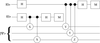
Figure 2: Circuit to measure the stabilizer generators $XIX$ and $YYZ$ for the $[[3,1]]$ QECC, (11). The top two wires are the error correction ancillas, while the bottom three wires are the code qubits. Time flows from left to right. The boxes $H$ and $M$ represent a Hadamard and measurement in the computational basis, respectively. The circle with an operation $U\in\{X,Y,Z\}$ represents a control-$U$ operation, with control at the filled circle on the other end of the “stick”. Only two-qubit interactions are used.

The state $\rho_{i}\equiv|\Psi_{L}\rangle\langle\Psi_{L}|$ transforms under this channel, as per Eq. (1), to $\rho_{f}=\sum_{m,n}\chi_{m,n}|\Psi^{m}_{L}\rangle\langle\Psi^{n}_{L}|=\frac{1}{4}[(2-\lambda+2\sqrt{1-\lambda})|\Psi_{L}\rangle\langle\Psi_{L}|+(2-\lambda-2\sqrt{1-\lambda})|\Psi^{Z}_{L}\rangle\langle\Psi^{Z}_{L}|+\lambda(|\Psi_{L}\rangle\langle\Psi^{Z}_{L}|+|\Psi^{Z}_{L}\rangle\langle\Psi_{L}|+|\Psi^{X}_{L}\rangle\langle\Psi^{X}_{L}|+|\Psi^{Y}_{L}\rangle\langle\Psi^{Y}_{L}|-i|\Psi^{X}_{L}\rangle\langle\Psi^{Y}_{L}|+i|\Psi^{Y}_{L}\rangle\langle\Psi^{X}_{L}|)].$ Syndrome measurements on this state yield the diagonal terms of $\chi$ as outcome probabilities. The only nonvanishing off-diagonal terms are $\chi_{I,Z}=\chi_{Z,I}=\lambda$ and $\chi_{X,Y}=-\chi_{X,Y}=-i\lambda$.

Suppose $U=U_{X,Y}\equiv\frac{X+Y}{\sqrt{2}}$ is applied to $\rho_{f}$, followed by measurement of the above two stabilizers. From Eq. (6), we see that this will reveal $\textrm{Re}(\chi_{X,Y})=0$ in the case of outcomes corresponding to errors $I$ and $Z$, and $\textrm{Im}(\chi_{I,Z})=0$ in the case of outcomes corresponding to errors $X$ and $Y$, so that $\lambda$ remains undetermined. To obtain information about $\textrm{Re}(\chi_{X,Y})$ or $\textrm{Im}(\chi_{I,Z})$, one applies prior to $U(X,Y)$, a toggling operation, which in the representation of the basis $\{|0_{L}\rangle,|0^{x}_{L}\rangle,|0^{y}\rangle,|0^{z}\rangle,|1_{L}\rangle,|1^{x}_{L}\rangle,|1^{y}\rangle,|1^{z}\rangle\}$, is given by the diagonal $8\times 8$ matrix:

$$S^{+}\equiv\frac{1}{\sqrt{2}}\left(\begin{array}[]{c|c}S&0\\ \hline\cr 0&S\end{array}\right),$$ (12)

where $S=\textrm{Diag}(\gamma,\overline{\gamma},\gamma,\overline{\gamma})$, with $\gamma=1+i$ and $\overline{\gamma}=1-i$. For the toggled channel, $\chi^{\prime}_{I,J}=\left(S\chi S\right)_{I,J}=i\chi_{I,J}=i\lambda$. Similarly, $\chi^{\prime}_{X,Y}=i\chi_{X,Y}=\lambda$. Thus the full noise is determined. The following three configurations are used for CQD: (i) immediate stabilizer measurement; (ii) pre-processing with $U(X,Y)$ before stabilizer measurement; (iii) pre-processing with $S^{+}$ and then $U(X,Y)$ before stabilizer measurement.

IV Discussion and Conclusions

We have proposed QECCD, a method for CQD that exploits QEC techniques. Like DCQD Mohseni and Lidar (2006), CQD is direct and requires a separation of a clean qubit system A from the noisy qubit system P. While this assumption is a bit restrictive, it is worth noting that all AAPT methods (to our knowledge) require this assumption. Expanding our method so that some noise is allowed in the ancillary system would be an interesting future direction of work. Another direction for expansion of our method would be to incorporate fault-tolerance, by allowing the gate operations performed during CQD to be imperfect. This approach may either aim to determine a threshold for the gate fidelity that would allow CQD to be accurate, or relate gate fidelity to the variance in the estimated noise parameters.

Unlike earlier CQD techniques, the QECCD protocol is not restricted to a fixed set of initial states, but accepts as input any encoded quantum information and, thus, can be implemented concurrently with the QCC. This has the economizing virtue that a quantum state used for CQD need not be discarded from the quantum computation procedure. Moreover, QECCD requires at most only twice the number of experimental configurations as does DCQD or AAPT with mutually unbiased basis measurements. Unlike AAPT with POVMs, which requires many-body interactions, QECCD, like DCQD, requires only one- and two-body interactions 12b .

We now highlight some other insights that our method has provided: First, we present in Eq. (2) a new channel-state isomorphism, which is similar to the Choi-Jamiolkowski isomorphism, but with an interesting twist. To turn the Choi-Jamiolkowski isomorphism into a method for CQD, one requires a full state tomography on the state obtained under the isomorphism (the Choi matrix). By our method, however, the QECC isomorphism only requires partial information (syndrome outcome data) at each step.

Second, QEC involves destroying the coherence between Pauli errors, and only gives the probability of those errors. Nevertheless, the QECC isomorphism, (2), implies that the noisy encoded state contains these coherence data, and raises the question whether this coherence information can be physically accessed using QEC techniques. Our method answers this question in the affirmative.

Third, some of the mathematical tools we propose, such as toggling to determine the real and imaginary parts of the off-diagonal terms of the density operator, can be of independent interest.

Last but not least, the QECCs which we introduced for QECCD are different in that they are novel. They are stabilizer codes that correct arbitrary errors on known coordinates, and have the property that the set of allowed Pauli errors forms a group. Codes (3) and (11) are examples of such QECCs suitable for QECCD. Interestingly, both these codes are perfect.

References

- Nielsen and Chuang (2000) M. Nielsen and I. Chuang, Quantum Computation and Quantum Information (Cambridge University Press (Cambridge), 2000).
- D’Ariano (2000) Giacomo Mauro D’Ariano, “Quantum tomography: General theory and new experiments,” F. der Physik 48, 579–588 (2000).
- Altepeter et al. (2003) J. B. Altepeter, D. Branning, E. Jeffrey, T. C. Wei, P. G. Kwiat, R. T. Thew, J. L. O’Brien, M. A.Nielsen, and A. G. White, “Ancilla-assisted quantum process tomography,” Phys. Rev. Lett. 90, 193601 (2003).
- Mohseni and Lidar (2006) M. Mohseni and D. A. Lidar, “Direct characterization of quantum dynamics,” Phys. Rev. Lett. 97, 170501 (2006).
- Mohseni and Lidar (2007) M. Mohseni and D. A. Lidar, “Direct characterization of quantum dynamics: General theory,” Phys. Rev. A 75, 062331 (2007).
- Emerson et al. (2007) Joseph Emerson et al., “Symmetrized characterization of noisy quantum processes,” Science 317, 1893–1896 (2007).
- Silva et al. (2008) M. Silva, E. Magesan, D. W. Kribs, and J. Emerson, “Scalable protocol for identification of correctable codes,” Phys. Rev. A 78, 012347 (2008).
- (8) Austin G. Fowler, D. Sank, J. Kelly, R. Barends, and John M. Martinis, ArXiv:1405.1454.
- (9) J. Combes, C. Ferrie, C. Cesare, M. Tiersch, G. J. Milburn, H. J. Briegel, and C. M. Caves, ArXiv:1405.5656.
- (10) Y. Fujiwara, ArXiv:1405.6267.
- Bendersky et al. (2008) Ariel Bendersky, Fernando Pastawski, and Juan Pablo Paz, “Selective and efficient estimation of parameters for quantum process tomography,” Phys. Rev. Lett. 100, 190403 (2008).
- Shabani and Lidar (2009) Alireza Shabani and Daniel A. Lidar, “Maps for general open quantum systems and a theory of linear quantum error correction,” Phys. Rev. A 80, 012309 (2009).
- (13) D. Gottesman, ArXiv:0904.2557.
- Omkar et al. (2013) S. Omkar, R. Srikanth, and Subhashish Banerjee, “Dissipative and non-dissipative single-qubit channels: dynamics and geometry,” Quant. Info. Proc. 12, 3725 (2013).
- Laflamme et al. (1996) Raymond Laflamme, Cesar Miquel, Juan Pablo Paz, and Wojciech Hubert Zurek, “Perfect quantum error correcting code,” Phys. Rev. Lett. 77, 198–201 (1996).
- Shukla et al. (2013) Abhishek Shukla, K. Rama Koteswara Rao, and T. S. Mahesh, “Ancilla-assisted quantum state tomography in multiqubit registers,” Phys. Rev. A 87, 062317 (2013).
- Knill et al. (2001) E. Knill, R. Laflamme, and G. J. Milburn, Nature 409, 46–52 (2001).
- (18) All stabilizer measurements and error correction operations can be implemented using one- and two-body interactions Gupta et al. (2007). To see that such interactions suffice to implement and , consider the unitary version of QEC, which requires only one- and two-body interactions and can be represented as: where the first register is the computer and the second holds the syndrome register. To implement , one prepares the second register (an ancilla) in the state and reverses the above operation. To implement one corrects the state of the quantum computer, applies the phase gate on the second register, and then “uncorrects” the resulting composite system. For the last step, we invoke the result that single qubit gates and CNOT are universal for quantum computation Nielsen and Chuang (2000).
- Gupta et al. (2007) M. Gupta, A. Pathak, R. Srikanth, and P. K. Panigrahi, “General circuits for indirecting and distributing measurement in quantum computation,” Int. Journal of Quantum Information 5, 627 (2007).