Spin-Orbit angle distribution
and the origin of (mis)aligned hot Jupiters

Abstract

Context. For 61 transiting hot Jupiters, the projection of the angle between the orbital plane and the stellar equator (called the spin-orbit angle) has been measured. For about half of them, a significant misalignment is detected, and retrograde planets have been observed. This challenges scenarios of the formation of hot Jupiters.

Aims. In order to better constrain formation models, we relate the distribution of the real spin-orbit angle $\Psi$ to the projected one $\beta$. Then, a comparison with the observations is relevant.

Methods. We analyse the geometry of the problem to link analytically the projected angle $\beta$ to the real spin-orbit angle $\Psi$. The distribution of $\Psi$ expected in various models is taken from the literature, or derived with a simplified model and Monte-Carlo simulations in the case of the disk-torquing mechanism.

Results. An easy formula to compute the probability density function (PDF) of $\beta$ knowing the PDF of $\Psi$ is provided. All models tested here look compatible with the observed distribution beyond 40 degrees, which is so far poorly constrained by only 18 observations. But only the disk-torquing mechanism can account for the excess of aligned hot Jupiters, provided that the torquing is not always efficient. This is the case if the exciting binaries have semi-major axes as large as $\sim 10^{4}$ AU.

Conclusions. Based on comparison with the set of observations available today, scattering models and the Kozai cycle with tidal friction models can not be solely responsible for the production of all hot Jupiters. Conversely, the presently observed distribution of the spin-orbit angles is compatible with most hot Jupiters having been transported by smooth migration inside a proto-planetary disk, itself possibly torqued by a companion.

1 Introduction

The existence of close-in giant planets whose orbits lie in close proximity to their host stars is now well established (e.g., Cumming, 2011). Although these objects constitute the best observationally characterised sample of exoplanets, their origins remain puzzling from a theoretical point of view. As in-situ formation of hot Jupiters is problematic (Chiang & Laughlin, 2013), it is likely that these objects have formed beyond the ice-line in the proto-planetary disk (i.e, at an orbital separation of a few AU) and have since been transported inwards (Lin et al., 1996). Traditionally, smooth migration forced by interaction with the proto-planetary disc in which planets form, has been invoked to facilitate transport (Lin & Papaloizou, 1986; Lin et al., 1996; Wu & Murray, 2003; Crida & Morbidelli, 2007; Papaloizou et al., 2007). Recently, substantially more violent processes have been proposed to account for the generation of hot Jupiters (Fabrycky & Tremaine, 2007; Nagasawa et al., 2008; Beaugé & Nesvorný, 2012). However, the dominance of the roles played by each mechanism remains controversial (Dawson et al., 2012). Accordingly, observations of the stellar spin-planetary orbit misalignment has been invoked as a means of differentiating among the proposed models.

Among the $\sim 1000$ exoplanets detected to date, $\sim 60$ have an observed measure of the angle between their orbital plane and the equatorial plane of their host star (e.g., Winn et al., 2007; Triaud et al., 2010). Traditionally, this has been achieved through the Rossiter-McLaughlin effect (Mac Laughlin, 1924) ; however, recently novel techniques involving asteroseismology (Huber et al., 2013) and star-spot measurements (Hirano et al., 2012) have also been utilised to this end. A wide variety of measured angles have been reported to date, and many exo-planets are apparently characterised by spin-orbit misalignment : the orbital obliquity differs significantly from $0$. Instinctively, this is surprising as planets are supposed to form within a proto-planetary disk whose angular momentum direction is the same as that of the star. Therefore, the origin of the spin-orbit misalignment has received considerable attention over the past few years.

A promising way to disentangle the roles of the various transport mechanisms, is to analyse the observed distribution of the spin-orbit angles, and to compare it to the expected distribution from a given model. However, observations only provide the projected spin-orbit angle, not the real one. Accordingly, in section 2, we describe the 3D geometry of the problem, and we infer the distribution of the projected spin-orbit angles from the real ones (and vice-versa).

In section 3, we compute the distributions of the projected spin-orbit angles expected from various mechanisms, devoting special attention to the disk-torquing model (Batygin, 2012). Within the framework of the disk-torquing mechanism, a (possibly transient) companion to a young star makes the proto-planetary disk precess around the binary’s axis, so that the plane in which planets eventually form and the equatorial plane of the central star can differ. Contrary to the violent category of migration mechanisms – e.g., planet-planet scattering (Rasio & Ford, 1996; Ford & Rasio, 2008) and Kozai resonance (Wu & Murray, 2003; Fabrycky & Tremaine, 2007; Naoz et al., 2011) – this process predicts that all the planets of the system can share the same misalignment. The recent discovery of significant misalignment among a multi-transiting system (Huber et al., 2013) therefore puts emphasis on this model.

Using analytical arguments and Monte-Carlo simulations, we find that the current observational aggregate can be well explained by the disk-torquing effect, implying that disk-driven planet migration in (torqued) disks could be the dominant source of (mis)aligned hot Jupiters.

2 The 3D geometry of the spin-orbit angle

There is considerable confusion in the literature about the spin-orbit angle. Let us define precisely what we are interested in here. The true misalignment angle is actually the angle between two vectors in 3D space : $\@vec{L}_{p}$, the orbital angular momentum of the planet, and $\@vec{L}_{s}$, the angular momentum of the spin of the star. As such, it can only lie between $0$ and $180$ degrees (there are no negative angles in 3D). This real, 3D angle is denoted below as $\Psi$.

The projections of these two vectors onto the plane of the sky (noted $\@vec{L}_{p}^{\prime}$ and $\@vec{L}_{s}^{\prime}$) form an oriented angle, which in principle could range between $-180^{\circ}$ and $+180^{\circ}$. However, whether the angle ($\@vec{L}_{p}^{\prime},\@vec{L}_{s}^{\prime}$) is positive or negative when measured clockwise, corresponds to the same 3D configuration, observed from either side of the star, from the ascending or descending node. In any case, the two cases are indistinguishable observationally (Triaud, personal communication). Thus, it does not make sense to report negative angles. The projected spin-orbit angle should also be expressed as between $0^{\circ}$ and $180^{\circ}$. Still, on exoplanets.org, one finds many negative projected spin-orbit angles, taken from published articles. This angle is sometimes noted $\lambda$ (e.g., Fabrycky & Winn, 2009, exoplanets.org), and sometimes it is noted as $\beta$ (e.g., Triaud et al., 2010). The projected angle is denoted below as $\beta$, and will be taken as the absolute value of the misalignment angle $\beta$ or $\lambda$ reported in the literature.

2.1 Relation between the real and projected spin-orbit angle

Assume that $\Psi$ is fixed. Which $\beta$ will be observed ? What is the probability density function (PDF) of $\beta$ ?

This question has already been addressed in general by Fabrycky & Winn (2009). They provide $\beta$ (that they note $\lambda$) as a function of $\Psi$ and $i_{o}$, the inclination of the orbital angular momentum with respect to the line of sight. Here, we propose a simpler, one column derivation, making the assumption that the observer is exactly in the orbital plane ($i_{o}=\pi/2$) ; this is appropriate because all the planets with known spin-orbit angle transit their host star, so $|\pi/2-i_{o}|$ is very small. In this case, $\@vec{L}_{p}=\@vec{L}_{p}^{\prime}$ is perpendicular to the line of sight, and is in the plane of the sky. Let us consider spherical coordinates ($r,\phi,\theta$) centred on the star, such that colatitude $\theta=0$ corresponds to the north pole of the orbit, the direction of $\@vec{L}_{p}$ ; the origin of the longitude ($\theta=90^{\circ}$, $\phi=0$) corresponds to the direction of the observer. In these coordinates, $\@vec{L}_{s}$ has a colatitude $\theta_{s}=\Psi$. Its azimuth $\phi_{s}$ can be anything between $0$ and $2\pi$, with a uniform distribution. Clearly, if $\phi_{s}\equiv 0[\pi]$, the observer sees $\beta=0$ if $\Psi<\pi/2$, and $\beta=\pi$ if $\Psi>\pi/2$ ; conversely, if and only if $\phi_{s}=\pm\pi/2$ the observer sees $\beta=\Psi$ exactly.

This configuration is shown in the right panel of Figure 1. The point $O$ is the centre of the unit sphere, and $P$ and $S$ are the intersection of the sphere with the vectors $\@vec{L}_{p}$ and $\@vec{L}_{s}$ respectively. The point $A$ has colatitude $\theta=\Psi$ and azimuth $\phi=0$, facing the observer, while $R$ has colatitude $\theta=\Psi$ and azimuth $\phi=\pi/2$, appearing on the limb of the star for the observer. Accordingly, $OA=OS=OP=OR=1$ .

The plane $(OPR)$ is the plane perpendicular to the line of sight passing through $O$ : it is the plane of the sky as seen by the observer, onto which everything is orthogonally projected, along the direction of the line of sight.

The circle gathering all the points with colatitude $\Psi$ is the dashed circle passing through $A$, $S$, and $R$. This circle is represented in the top left of Figure 1. The orthogonal projections of $A$ and $S$ onto the plane $(OPR)$, are $A^{\prime}$ and $S^{\prime}$ respectively. The centre of this dashed circle is $A^{\prime}$, and its radius is obviously $A^{\prime}A=A^{\prime}S=A^{\prime}R=\sin\Psi$. Thus, $A^{\prime}S^{\prime}=\sin\Psi\,|\sin\phi_{s}|$.

In the projected plane (shown in bottom left of Fig. 1), the angle between the north pole of the orbit and the spin of the star appears to be $\beta=\widehat{POS^{\prime}}$. As $A^{\prime}$ is the orthogonal projection of $S^{\prime}$ on the $(OP)$ line, we have $\tan\beta=A^{\prime}S^{\prime}/OA^{\prime}$, where $OA^{\prime}=\cos\Psi$ is negative when $\Psi>\pi/2$. Finally,

$$\beta = \arctan\left(|\sin\phi_{s}|\,\tan\Psi\right)\equiv G(\phi_{s})$$ (1)

$$|\phi_{s}| = \arcsin\left(\frac{\tan\beta}{\tan\Psi}\right)\ .$$ (2)

This is equivalent to Eq. (11) of Fabrycky & Winn (2009), with $i_{o}=\pi/2$, $\Omega=\phi_{s}$ and $\lambda=\beta$.

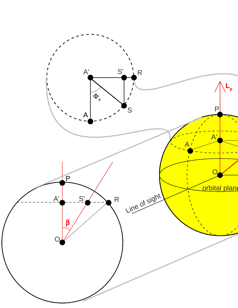
Figure 1: Right : 3D representation of the problem. The yellow sphere is the unit sphere centred on the star. P marks the direction of the orbital angular momentum vector $\@vec{L}_{p}$ and S that of the stellar spin $\@vec{L}_{s}$. The dashed circle passing through points A and S gathers all the points making an angle $\Psi$ with P. It is represented in the top left.
Top left : The circle of the unit sphere gathering all the points at colatitude $\Psi$ with respect to the orbital angular momentum vector of the planet. A is the point facing the observer ; S is the point corresponding to the direction of the stellar spin. A and S are projected on the diameter of this circle perpendicular to the line of sight onto A’ and S’ ; $\phi_{s}$ is then $\widehat{AA^{\prime}S}$.
Bottom left : The projected plane, as seen by the observer. The previous dashed circle is now a dashed horizontal line, on which A’ and S’ are the projections of A and S along the direction of the line of sight. The arc PR defines an angle $\Psi$, while the projected spin orbit angle $\beta$ is $\widehat{A^{\prime}OS^{\prime}}$, marked in red.

2.2 Probability density function of $\beta$, for fixed $\Psi$

Now, as the distribution of $\phi_{s}$ is uniform in the interval $[0;2\pi[$, and $|\sin(x)|=|\sin(\pi-x)|=|\sin(\pi+x)|=|\sin(2\pi-x)|$, it is sufficient to consider a uniform distribution for $0\leqslant\phi_{s}<\pi/2$, with probability density $2/\pi$. In this case, $\beta$ is a monotonic function of $\phi_{s}$. It is well known that if $X$ is a random variable of probability density function $f_{X}$, and $Y=G(X)$ with G a monotonic function, then the PDF of $Y$ is

$$f_{Y}(y)=f_{X}\left(G^{-1}(y)\right)\times\left|\left(G^{-1}\right)^{\prime}(y)\right|\ .$$ (3)

Thus, using Eq. (1) for fixed $\Psi$, the PDF of $\beta$ is :

$$f(\beta|\Psi)=\left\{\begin{array}[]{ll}\displaystyle\frac{2}{\pi}\frac{1+\tan^{2}\beta}{(\tan^{2}\Psi-\tan^{2}\beta)^{1/2}}&{\rm if\ }\beta\in\mathcal{T}\ ,\vspace{3pt}\\ 0&{\rm otherwise}\end{array}\right.$$ (4)

where $\mathcal{T}=\{0\leqslant\beta<\Psi<\frac{\pi}{2}\}\cup\{\frac{\pi}{2}<\Psi<\beta\leqslant\pi\}$.

This equation is identical to Eq. (19) of Fabrycky & Winn (2009).

Figure 2 shows the decimal logarithm of $f(\beta|\Psi)$ in the $\beta-\Psi$ plane. For a given real spin-orbit angle $\Psi_{0}$, the PDF of the observed projected angle $\beta$ can be found by going along a $\Psi=\Psi_{0}$ line in the figure. One can check analytically that for all $\Psi$, $\displaystyle\int_{\beta=0}^{\beta=\pi}f(\beta|\Psi)\,{\rm d}\beta=1$ , as it should.

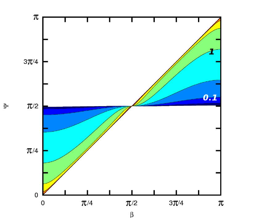
Figure 2: Contour map of $f(\beta|\Psi)$ as defined by Eq. (4). The contours correspond to values $10^{k}$, with $k=-1.5,\,-1\ldots 1,\,1.5$ ; the curves corresponding to $f=1$ and $f=0.1$ are marked. Note that $f$ actually diverges towards $+\infty$ approaching the $\Psi=\beta$ line.

2.3 Conversion of the PDF of $\Psi$ into the PDF of $\beta$

If now $\Psi$ has its own PDF $w(\Psi)$, the corresponding PDF of $\beta$ will be :

$$f(\beta)=\int_{\Psi=0}^{\Psi=\pi}f(\beta|\Psi)w(\Psi)\ {\rm d}\Psi\ .$$ (5)

Computing this integration corresponds to summing vertically in Figure 2, after having given to every horizontal line a weight $w(\Psi)$.

For example, assuming a uniform $w(\Psi)=1/\pi$, one gets the double-peaked distribution shown in Fig. 3. On the other hand, assuming that $\Psi$ is isotropically distributed, $w(\Psi)=(\sin{\Psi})/2$, one can solve Eq. (5) and find $f(\beta)=1/\pi$, uniform, as expected. The observed distribution of $\beta$ (see histogram in Fig. 5) is neither flat nor reminiscent of the distribution shown in Fig. 3, implying that the real distribution of $\Psi$ is neither uniform, nor isotropic.

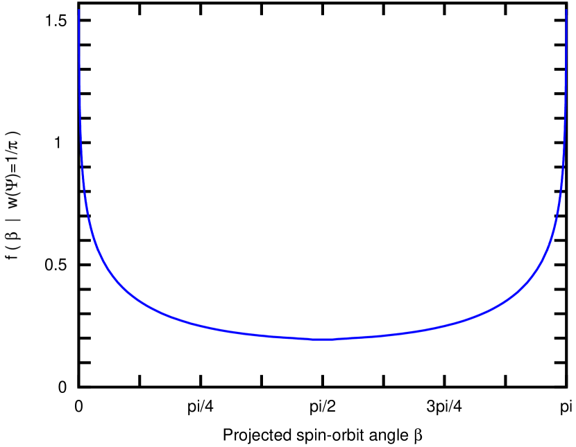
Figure 3: Representation $f(\beta)$ when $w(\Psi)=1/\pi$ (uniform distribution of $\Psi$).

2.4 Deprojection

Let $i_{s}$ be the angle between the stellar angular momentum $\@vec{L_{s}}$ and the line of sight ; an isotropic distribution of $\@vec{L_{s}}$ on the unit sphere gives to $i_{s}$ a PDF $f(i_{s})=\frac{1}{2}\sin(i_{s})$ between $0$ and $\pi$. On the projected plane (bottom left of figure 1), we now have $OS^{\prime}=\sin i_{s}$, and $OA^{\prime}=OS^{\prime}\times\cos\beta=OR\times\cos\Psi=\cos\Psi$. Thus,

$$\Psi=\arccos(\cos\beta\times\sin i_{s})=G_{2}(i_{s})\ .$$ (6)

Note that $i_{s}$ or $\pi-i_{s}$ give exactly the same projection. One can therefore assume that $i_{s}$ is distributed between $0$ and $\pi/2$ with PDF $f(i_{s})=\sin(i_{s})$. Then, using Eqs. (3) and (6), one gets :

$$f(\Psi|\beta)=\left\{\begin{array}[]{ll}\vspace{6pt}\frac{\cos\Psi}{\cos\beta}\frac{\sin\Psi}{\sqrt{\cos^{2}\beta-\cos^{2}\Psi}}&\begin{array}[]{l}{\rm if\ }\ 0<\beta<\Psi<\pi/2\\ {\rm or\ }\pi/2<\Psi<\beta<\pi\ ,\end{array}\\ 0&\begin{array}[]{l}{\rm otherwise\ ,}\end{array}\end{array}\right.$$ (7)

in agreement with Eq. (21) of Fabrycky & Winn (2009).

Then, the PDF of $\Psi$ can be deduced from the observations of $\beta$ :

$$f(\Psi)=\sum_{i}f(\Psi|\beta_{i})$$ (8)

where the index $i$ spans the whole sample.

Applying this to the data found on exoplanets.org at the end of 2013, we get an irregular curve peaked at each of the $\beta_{i}$, as $f(\Psi|\beta_{i})$ diverges towards $+\infty$ as $\Psi\to\beta_{i}$. This curve is displayed as a thin blue line in Figure 4. To avoid this, one could smooth the data using the error-bars $\sigma_{i}$ and compute :

$$f(\Psi)=\sum_{i}\int\frac{1}{\sqrt{2\pi}\sigma_{i}}\exp\left(-\frac{(\beta-\beta_{i})^{2}}{2\,{\sigma_{i}}^{2}}\right)\ f(\Psi|\beta)\ {\rm d}\beta\ .$$

However, the $\sigma_{i}$ are so diverse (from $0.3$ to $60^{\circ}$) that this operation would only degrade the information, without completely smoothing the curve. Therefore, we prefer to operate similar to the observations of $\beta$ and build a histogram : we average $f(\Psi)$ on successive intervals of $20^{\circ}$ width. This is represented in Figure 4 as the red stairs, while the histogram of the observations of $\beta$ is shaded grey. It seems here that aligned hot Jupiters are a minority. However, one should realize that if all hot Jupiters were actually aligned, $\Psi=\beta=0$, but Eq (7) gives $f(\Psi|\beta=0)=\textrm{max}\{\cos\Psi\,,\,0\}$ ; it is therefore almost impossible that the first step of the red stairs is the highest step, even if there is a large majority of aligned hot Jupiters.

In any case, with only $18$ cases with $\beta>40^{\circ}$ in the data, and large error bars, the statistics is rather poor to infer the PDF of $\Psi$ accurately. Therefore, in what follows, we prefer to infer the PDF of $\beta$ from various mechanisms, and compare it directly with the observed distribution of $\beta$.

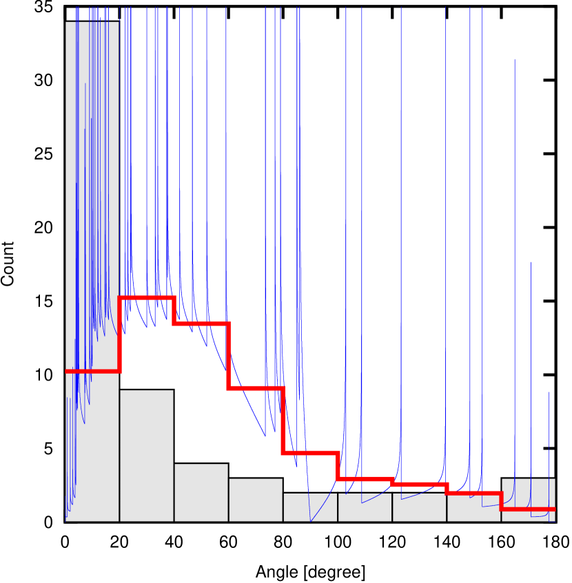
Figure 4: Grey shaded histogram : distribution of the observed projected spin-orbit angle $\beta$ (taken as $|\beta|$ or $|\lambda|$ in the data from exoplanets.org). Blue thin curve : $f(\Psi)$, as given by Eq. (8). Red stairs : Histogram of the PDF of $\Psi$ with bins of $20^{\circ}$.

3 Application to proposed mechanisms

In this section, we compute/take the PDF of $\Psi$ that is expected from several mechanisms of formation of hot Jupiters. Then, we compute the corresponding PDF of $\beta$ using Eq. (5), and compare it with the distribution of the observations. The distribution of the observations is shown as a grey shaded histogram in Figures 5, 7, and 8. The bins have a width of $20^{\circ}$, and many of them contain only two cases. This small number statistics is prone to significant variations with new observations, or change of the bins : one object more or less in a bin represents a $50\%$ variation. Nonetheless, it appears robust that the distribution of the projected spin-orbit angle beyond $60^{\circ}$ is almost uniform. Models should account for this.

To be more precise, assuming the small number of planets in our bins follows a Poisson process of parameter $\lambda$, when $N$ are found in a bin, the likelihood of $\lambda$ is given by $\lambda^{N}\exp(-\lambda)/N!$ . Thus, in the bins where two are found, one can say with $50\%$ confidence that $1.17<\lambda<3.16$ and with $95\%$ confidence that $0.31<\lambda<6.34$.

3.1 Disk torquing

Contemporary observational surveys suggest that a considerable fraction of solar-type stars are born as binary or multiple systems (Ghez et al., 1993; Kraus et al., 2011). Moreover, most stars form in embedded cluster environments (Lada & Lada, 2003) where dynamical evolution can lead to the acquisition of transient companions (Malmberg et al., 2007). Recently, Batygin (2012) showed that the presence of a companion to a young star can force the proto-planetary disk to precess around the binary’s axis, so that the plane in which planets eventually form and the equatorial plane of the central star can differ.

3.1.1 Analytic simple model

Denoting the angle between the orbital plane of the companion and the stellar equator as $i\,^{\prime}$ (therefore, $0\leqslant i\,^{\prime}\leqslant\pi/2$), $\Psi$ evolves between $0$ and $2i\,^{\prime}$ in this mechanism. At first sight of Fig. 2 of Batygin (2012), it seems reasonable to consider this evolution as linear with time, back and forth. In the end, the PDF of $\Psi$ is a uniform distribution between $0$ and $2i\,^{\prime}$ :

$$f(\Psi\,|\,i\,^{\prime})=\frac{1}{2i\,^{\prime}}\ \textrm{\ if\ }0\leqslant\Psi\leqslant 2i\,^{\prime}\ ;\ \ 0\textrm{\ otherwise.}$$ (9)

The PDF of $i\,^{\prime}$ should correspond to an isotropic distribution of the orbital angular momentum vector of the companion with respect to the stellar spin, thus it reads :

$$g(i\,^{\prime})=\sin(i\,^{\prime})\ .$$ (10)

Now, the PDF of $\Psi$ is given by :

$$f_{B12}(\Psi) = \int_{0}^{\pi/2}f(\Psi\,|\,i\,^{\prime})g(i\,^{\prime})\ {\rm d}i\,^{\prime}$$

$$= \int_{\Psi/2}^{\pi/2}\frac{\sin(i\,^{\prime})}{2i\,^{\prime}}\,{\rm d}i\,^{\prime}$$

$$f_{B12}(\Psi) = \frac{1}{2}\left[\textrm{Si}(\pi/2)-\textrm{Si}(\Psi/2)\right]$$ (11)

where $\mathrm{Si}(x)=\int_{0}^{x}\frac{\sin(t)}{t}\,{\rm d}t$, which has unfortunately no easy analytical expression. Nonetheless, this expression can be computed numerically. On Figure 5, $f_{B12}$ is displayed as the red thin curve ; it looks linear, but it’s actually not a straight line. The corresponding PDF of $\beta$ (using Eq. (5) ) is shown as the blue thick curve. The major difference between the two curves enlights the necessity of taking the projection into account. In the background, the histogram of the observations shows a good agreement with the predicted distribution of the projected angles. The PDF of $\beta$ is normalised to have $18$ planets with $\beta>40^{\circ}$, like the data.

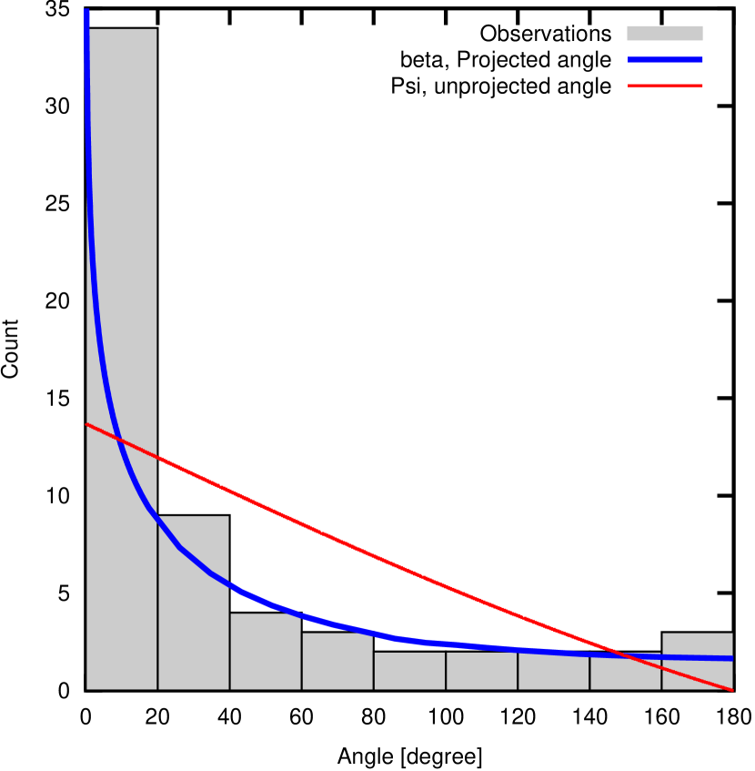
Figure 5: Distribution of the spin - orbit angle expected in the disk-torquing mechanism. Red thin line : distribution of $\Psi$, given by Eq. (11). Blue thick line : corresponding PDF of $\beta$. Background histogram : observations.

With this normalisation, the number of planets with $\beta<20^{\circ}$ (resp. $20^{\circ}<\beta<40^{\circ}$) is only $14.2$ (resp. $6.8$), while $34$ (resp. $9$) are observed. This excess of aligned planets in the observations should not bother us. Indeed, hot Jupiters form in the proto-planetary disk, and migrate inwards irrespective of the multiplicity of the stellar system. Thus, if the proto-planetary disk is not torqued (e.g., the star is always single), the hot Jupiters are expected to be aligned. If the proto-planetary disk is torqued by a companion, then the planets will be misaligned, with the distribution given above. The apparent excess of aligned hot Jupiter can therefore be interpreted as the fraction of disks that were never significantly torqued. We come back on this issue in the next sub-section.

3.1.2 Monte Carlo simulations

Within the framework of the model proposed by Batygin (2012), the stellar spin axis is taken to remain in the primordial plane of the disk for all time. Physically, this simplifying assumption corresponds to a non-accreting, unmagnetised young stellar object that rotates at a negligibly slow rate. This picture is somewhat contrary to real pre-main-sequence stars, which typically accrete $\sim 10^{-8}M_{\odot}$/year from the disk (Hartmann, 2008; Hillenbrand, 2008), have $\sim 1$ kGauss magnetic fields at the stellar surface (Shu et al., 1994; Gregory et al., 2010), and rotate with characteristic periods in the range $P_{\rm{rot}}\simeq 1-10$ days (Herbst et al., 2007). Accordingly, Batygin & Adams (2013) examined magnetically and gravitationally facilitated disk-star angular momentum transfer with an eye towards constraining the conditions needed for the acquisition of spin-orbit misalignment. They showed that the excitation of spin-orbit misalignment is only quenched when the host star continuously spins up because of gravitational contraction (i.e., the stellar field is too weak for magnetic breaking to occur ; see Shu et al., 1994; Matt & Pudritz, 2005a, b). However, they also found that the process by which spin-orbit misalignment is attained is somewhat more complicated than that described in Batygin (2012). Specifically, as the disk mass decreases throughout its lifetime, the gravitational coupling between the star’s quadrupole moment (that arises from rotational deformation) and the torqued disk gives rise to orbital obliquity via a secular resonance encounter between the stellar spin-axis precession frequency and the disk-torquing frequency (see Batygin & Adams, 2013, for details).

Cumulatively, the more complete model of Batygin & Adams (2013) does not easily lend itself to analytic manipulation. As a result, to derive the associated distribution of projected misalignment angles, we perform a Monte Carlo simulation, utilising their perturbative model (for brevity, we shall not rehash their formalism here, but instead refer the reader to their description). As above, the inclinations of the binary companion stars are taken to be isotropic, the binary semi-major axis is drawn from a log-flat distribution spanning $10^{2.5}-a_{\rm max}$ AU (where $a_{\rm max}$ can vary, see caption of Figure 6 ; Kraus et al., 2011), while the eccentricity and the primary-to-perturber mass ratio are taken to be uniform in the intervals [0,1] and [0.1,10], respectively (see Kraus et al., 2008). The primary star’s mass and the disk’s initial mass are also drawn from uniform distribution spanning [0.5,1.5] $M_{\odot}$ and [0.01,0.05] $M_{\odot}$, respectively (Herczeg & Hillenbrand, 2008). For all simulations, a surface density profile of the form $\Sigma\propto r^{-1}$ is assumed. The disk’s outer edge is taken to lie between $10^{1.5}$ and $10^{2}$ AU (Levison et al., 2008; Anderson et al., 2013), while the inner edge corresponds to the stellar corotation radius (Koenigl, 1991; Shu et al., 1994). In turn, the stellar rotation periods are randomly chosen to lie between 1 and 10 days in rough agreement with the observational samples of Littlefair et al. (2010); Affer et al. (2013). Following Gallet & Bouvier (2013), pre-main sequence rotational evolution is ignored because of the inherent complexities. Finally, the disk mass loss, stellar structure, and stellar gravitational contraction are modelled as described in Batygin & Adams (2013).

With the aforementioned ingredients in place, we compute the disk-torquing frequency as described in Batygin (2012, see equations 6 & 7 in the SI), while the rest of the calculation follows directly from section 4 of Batygin & Adams (2013). The results are shown in Figure 6. One thousand random sets of parameters have been chosen with the distributions described above, and the resulting $1000$ final spin - orbit angles have been binned in bins of $20^{\circ}$ width to produce a histogram, to be compared to the observations (Figure 5). Three cases are presented, where the only difference is the assumed value of $a_{\rm max}$, the maximum possible value of the semi-major axis of the binary ; from left to right, $a_{\rm max}=10^{3}$, $10^{3.75}$, and $10^{4.5}$ AU. The fraction of disks that will experience a negligible torquing appears to be very sensitive to $a_{\rm max}$. However, the distribution of the angles in the torqued cases remains unchanged, and close to the observations, as can be seen in Figure 7. In this figure, the three distributions obtained by the three sets of Monte Carlo simulations have been normalised to have $18$ planets with $\beta>40^{\circ}$, like in the data. They are represented in blue, green, and red stairs, and are very similar beyond $40^{\circ}$. In the background, the histogram of the data is shown in grey bars. All the three stairs are within 1 count of the histogram, signaling excellent agreement.

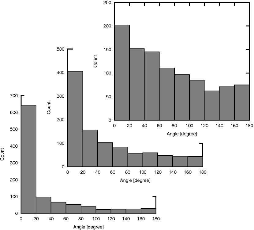
Figure 6: Distributions of the projected spin - orbit angle found in Monte Carlo simulations as described in the text, for three values of the maximum of the log-flat distribution of the semi-major axis of the binary. Top right : $a_{\rm max}=10^{3}$ AU. Middle : $a_{\rm max}=10^{3.75}$ AU. Bottom left : $a_{\rm max}=10^{4.5}$ AU.

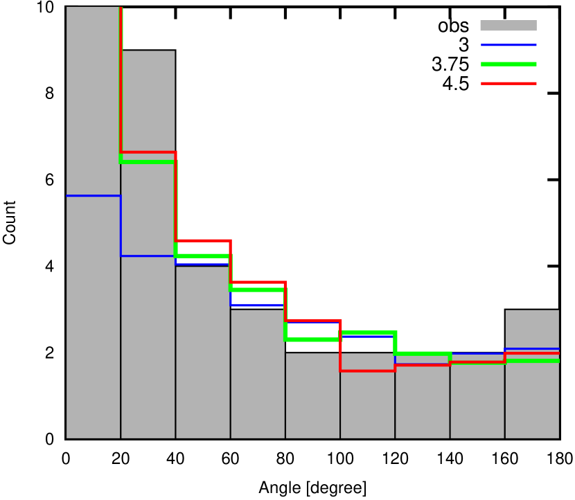
Figure 7: Distributions produced by the Monte Carlo simulations, normalised to $18$ cases with $\beta>40^{\circ}$. Thin blue : $a_{\rm max}=10^{3}$ AU. Thick green : $a_{\rm max}=10^{3.75}$ AU. Red : $a_{\rm max}=10^{4.5}$ AU. Background histogram : observations.

The choices of input parameters employed in the simulations are essentially naive estimates, predominantly guided by observational surveys. The observed agreement between the data and the model is thus compelling. However, with a considerable number of marginally constrained (and in some cases poorly understood) values at hand, it would not come as a surprise if the utilised model admitted significant variability in the distributions it could produce. Although a complete search of the parameter space is well beyond the scope of this study, it is noteworthy (as already alluded to above) that the model appears to be most sensitive to the orbital distribution of binary companions. While the median widest allowed binary orbit ($10^{3.75}\simeq 5\,600$ AU) in the simulation was motivated by the observational study of Kraus et al. (2011), if we reduce this range to $10^{3\,}$AU, the enhancement near $\beta=0$ in Figure 6 disappears entirely. On the contrary, if the range is extended to $10^{4.5\,}$AU, the enhancement near aligned orbits grows by almost a factor of $\sim 2$, although in both cases the shape of the PDF in the significantly misaligned region remains unchanged. The physical reason behind this is not exceedingly difficult to understand. As binary orbits get wider, the free precession (i.e., torquing) frequency of the disk decreases. This allows stars to adiabatically trail their disks for extended periods of time (Batygin, 2012). In turn, this means that by the time the secular resonance encounter between the stellar spin-axis precession rate and the disk precession rate happens, the disk mass is systematically lower, leading to smaller excitation of misalignment.

Ideally, one would like to examine the sensitivity of the model to the assumed parameters in greater detail, although for such an activity to be meaningful, the underlying physics (particularly in the case of pre-main-sequence rotational evolution) must await some clarification. Therefore, we leave this exercise for a later study.

3.2 Other mechanisms

3.2.1 Perturbations to the planetary orbit

A few processes of formation of hot Jupiters have been proposed by several authors, who provide the expected distribution of the final inclination of the hot Jupiter with respect to its initial orbital plane. As already argued in Section 2, this angle should be $\Psi$ in the end. We have collected these data from the papers, and derived the expected distribution of the projected spin-orbit angle $\beta$. We refer the reader to the original papers for a detailed explanation of how the distributions of $\Psi$ were derived by the authors. The data is originally in the form of a histogram $(\alpha_{i},N_{i})$, where $\alpha_{i}$ is the angle at the centre of the bin, and $N_{i}$ the number of planets with $\Psi$ in this bin. From this, we constructed $f=\sum_{i}f(\beta|\Psi=\alpha_{i})N_{i}$, the distribution of $\beta$. We then bin $f$ using the same bins as in the original histogram. We checked that spreading the $N_{i}$ planets among angles different from $\alpha_{i}$ in the bin does not change the final histogram of $\beta$ significantly.

The results are shown in Figure 8. The red line with + symbols labelled F.T. 2007 represents the distribution of $\beta$ expected in the Fabrycky & Tremaine (2007) mechanism of Kozai cycles with tidal friction (their Fig. 10b providing $\Psi$ in bins of $10^{\circ}$). The blue line with stars labelled N.I.B.2008 corresponds to the distribution found by Nagasawa et al. (2008) in their model of planet-planet scattering, tidal circularisation, and Kozai mechanism ; the data is taken from their Figure 11c, which shows the histogram of $\Psi$ of formed close-in planets in all simulations, with bins of $0.1$ rad. The green line with circles labelled B.N.2012 corresponds to the distribution found by Beaugé & Nesvorný (2012) in their model of multi-planet scattering, in the case of three planets after 1 Gyrs of evolution (their fig. 16). All the distributions of $\beta$ have been normalised to have $18$ cases with $\beta>40^{\circ}$, for an easier comparison.

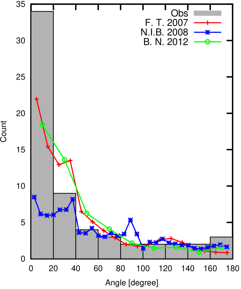
Figure 8: Distribution of $\beta$ expected from several mechanisms of forming hot Jupiters. Background histogram : observations.

The agreement between the curves and the histogram beyond $40^{\circ}$ is in general satisfactory. Based on the small number of planets observed in each bin, it seems impossible to exclude one or the other mechanism at present. However, none of these processes can individually account for the sharp peak at $\beta<20^{\circ}$. To this end, Beaugé & Nesvorný point out that “it is possible that the population of hot Jupiters with $\beta<20^{\circ}$ have a different origin”.

It should be noted, however, that Beaugé & Nesvorný (2012) had studied other scenarios, varying the inital number of planets, and the final age of the systems. Four different cases are shown in their paper, giving four different distributions. In particular, we have checked that the case with four planets, after 3 Gyr of evolution, once normalised to the $\beta>40^{\circ}$ cases, would give an excess of aligned hot Jupiters compared to the observations. Thus, one can not exclude that a combination of all the distributions matches the observations. We found that their four published distributions give an excess of planets in the $20^{\circ}<\beta<60^{\circ}$ range, but this concerns only four cases. Actually, the observations do sample the parameter space (in age and unknown initial conditions), so making a combination would be appropriate.

3.2.2 Perturbations to the stellar apparent spin

Along a completely different line of thought, Rogers et al. (2012, 2013) have proposed the misalignments to arise from the modulation of the outer layers of the host stars by interior gravity waves, rather than relics left behind by the dominant transport mechanism.

Cébron et al. (2011, 2013) also suggest that the excitation of the elliptical instability in the star by the tides raised by the planet could give an apparent tilted rotation axis. Even the total spin of the star could change direction, if the coupling with the planet is efficient. This will also lead to misalignment between a star and its hot Jupiter.

In order to assess the viability of these intriguing ideas, an expected distribution of spin-orbit angles should be generated within the framework of these models, and compared against the observed distribution via a treatment such as that presented in this work.

4 Discussion and conclusion

In this paper, we provide a simple derivation of the probability density function of the projected spin - orbit angle $\beta$, for fixed real spin - orbit angle $\Psi$. This allows us to link models (that produce distributions of $\Psi$) to observations (that measure $\beta$).

Firstly, our geometric description shows that only positive values for $\beta$ and $\Psi$ are sensible. These angles are between $0$ and $180^{\circ}$, where $\Psi=0$ corresponds to prograde aligned orbits, and $\Psi=180^{\circ}$ to retrograde aligned orbits. In particular, the notation $\lambda=-\beta$ often found in the litterature is irrelevant.

Second, we find that the observed distribution of $\beta$ presents a significant excess of quasi-aligned hot Jupiters ($\beta<20^{\circ}$) compared to the one expected from most models. This suggests that the scattering models and the Kozai cycle tidal friction models can not be solely responsible for the production of hot Jupiters. In previous studies (see Winn et al., 2010; Albrecht et al., 2012), the excess of nearly-aligned hot Jupiters has been attributed to tidal re-alignment of the star. However, Rogers & Lin (2013) recently pointed out that tidal re-alignment preferentially leads to prograde aligned, retrograde aligned, or orthogonal spin-orbit angles, in some contradiction with the observed distribution (Lai, 2012).

Third, in the simplest variant of the disk-torquing model, the over-representation of quasi-aligned planets is also not reproduced if the binaries responsible for the excitation of orbital obliquity have orbital semi-major axes smaller than $\sim 10^{3}$ AU. However, within the framework of the picture envisioned by Batygin & Adams (2013), alternative explanations are possible. These include adiabatic trailing of the host star, and early stripping or non-existance of the binary companion. In fact, the fraction of aligned disks increases dramatically with the maximum semi-major axes of the exciting binaries, $a_{\rm max}$. To this end, it is also worth noting that the wide binary fraction in star formation environments is a strong, growing function of primary stellar mass Kraus et al. (2011). Thus, a thorough investigation of the mass-dependence of the disk-torquing mechanism appears worthwhile.

On the other hand, the expected distribution of $\beta$ for $\beta>40^{\circ}$ in the disk-torquing model hardly depends on $a_{\rm max}$, and is in very good agreement with the observations. Although other parameters, poorly constrained, can have an influence on the distribution of $\Psi$ and $\beta$ in the disk-torquing mechanism, we can conclude that the presently observed distribution of the spin - orbit angles is compatible with most hot Jupiters having been transported by smooth migration inside a proto-planetary disk, possibly torqued by a companion.

Acknowledgments

K.B. acknowledges the generous support from the ITC Prize Postdoctoral Fellowship at the Institute for Theory and Computation, Harvard-Smithsonian Center for Astrophysics. This research has made use of the Exoplanet Orbit Database and the Exoplanet Data Explorer at exoplanets.org (Wright et al., 2011). We thank the referee C. Beaugé, as well as D. Nesvorny, for comments and suggestions that led to improvement of this article. We further thank S. Tremaine for having pointed out a mistake (now corrected) in our section 2.4.

References

- Affer et al. (2013) Affer, L., Micela, G., Favata, F., Flaccomio, E., & Bouvier, J. 2013, MNRAS, 430, 1433
- Albrecht et al. (2012) Albrecht, S., Winn, J. N., Johnson, J. A., et al. 2012, ApJ, 757, 18
- Anderson et al. (2013) Anderson, K. R., Adams, F. C., & Calvet, N. 2013, ApJ, 774, 9
- Batygin (2012) Batygin, K. 2012, Nature, 491, 418
- Batygin & Adams (2013) Batygin, K. & Adams, F. C. 2013, ArXiv e-prints
- Beaugé & Nesvorný (2012) Beaugé, C. & Nesvorný, D. 2012, ApJ, 751, 119
- Cébron et al. (2013) Cébron, D., Bars, M. L., Gal, P. L., et al. 2013, Icarus, 226, 1642
- Cébron et al. (2011) Cébron, D., Moutou, C., Le Bars, M., Le Gal, P., & Farès, R. 2011, in European Physical Journal Web of Conferences, Vol. 11, European Physical Journal Web of Conferences, 3003
- Chiang & Laughlin (2013) Chiang, E. & Laughlin, G. 2013, MNRAS, 431, 3444
- Crida & Morbidelli (2007) Crida, A. & Morbidelli, A. 2007, MNRAS, 377, 1324
- Cumming (2011) Cumming, A. 2011, Statistical Distribution of Exoplanets, ed. S. Seager, 191–214
- Dawson et al. (2012) Dawson, R. I., Murray-Clay, R. A., & Johnson, J. A. 2012, ArXiv e-prints
- Fabrycky & Tremaine (2007) Fabrycky, D. & Tremaine, S. 2007, ApJ, 669, 1298
- Fabrycky & Winn (2009) Fabrycky, D. C. & Winn, J. N. 2009, ApJ, 696, 1230
- Ford & Rasio (2008) Ford, E. B. & Rasio, F. A. 2008, ApJ, 686, 621
- Gallet & Bouvier (2013) Gallet, F. & Bouvier, J. 2013, A&A, 556, A36
- Ghez et al. (1993) Ghez, A. M., Neugebauer, G., & Matthews, K. 1993, AJ, 106, 2005
- Gregory et al. (2010) Gregory, S. G., Jardine, M., Gray, C. G., & Donati, J.-F. 2010, Reports on Progress in Physics, 73, 126901
- Hartmann (2008) Hartmann, L. 2008, Accretion Processes in Star Formation
- Herbst et al. (2007) Herbst, W., Eislöffel, J., Mundt, R., & Scholz, A. 2007, Protostars and Planets V, 297
- Herczeg & Hillenbrand (2008) Herczeg, G. J. & Hillenbrand, L. A. 2008, ApJ, 681, 594
- Hillenbrand (2008) Hillenbrand, L. A. 2008, Physica Scripta Volume T, 130, 014024
- Hirano et al. (2012) Hirano, T., Sanchis-Ojeda, R., Takeda, Y., et al. 2012, ApJ, 756, 66
- Huber et al. (2013) Huber, D., Carter, J. A., Barbieri, M., et al. 2013, Science, 342, 331
- Koenigl (1991) Koenigl, A. 1991, ApJ, 370, L39
- Kraus et al. (2011) Kraus, A. L., Ireland, M. J., Martinache, F., & Hillenbrand, L. A. 2011, ApJ, 731, 8
- Kraus et al. (2008) Kraus, A. L., Ireland, M. J., Martinache, F., & Lloyd, J. P. 2008, ApJ, 679, 762
- Lada & Lada (2003) Lada, C. J. & Lada, E. A. 2003, ARA&A, 41, 57
- Lai (2012) Lai, D. 2012, MNRAS, 423, 486
- Levison et al. (2008) Levison, H. F., Morbidelli, A., Van Laerhoven, C., Gomes, R., & Tsiganis, K. 2008, Icarus, 196, 258
- Lin et al. (1996) Lin, D. N. C., Bodenheimer, P., & Richardson, D. C. 1996, Nature, 380, 606
- Lin & Papaloizou (1986) Lin, D. N. C. & Papaloizou, J. 1986, ApJ, 309, 846
- Littlefair et al. (2010) Littlefair, S. P., Naylor, T., Mayne, N. J., Saunders, E. S., & Jeffries, R. D. 2010, MNRAS, 403, 545
- Mac Laughlin (1924) Mac Laughlin, D. B. 1924, ApJ, 60, 22
- Malmberg et al. (2007) Malmberg, D., de Angeli, F., Davies, M. B., et al. 2007, MNRAS, 378, 1207
- Matt & Pudritz (2005a) Matt, S. & Pudritz, R. E. 2005a, ApJ, 632, L135
- Matt & Pudritz (2005b) Matt, S. & Pudritz, R. E. 2005b, MNRAS, 356, 167
- Nagasawa et al. (2008) Nagasawa, M., Ida, S., & Bessho, T. 2008, ApJ, 678, 498
- Naoz et al. (2011) Naoz, S., Farr, W. M., Lithwick, Y., Rasio, F. A., & Teyssandier, J. 2011, Nature, 473, 187
- Papaloizou et al. (2007) Papaloizou, J. C. B., Nelson, R. P., Kley, W., Masset, F. S., & Artymowicz, P. 2007, in Protostars and Planets V, 655–668
- Rasio & Ford (1996) Rasio, F. A. & Ford, E. B. 1996, Science, 274, 954
- Rogers & Lin (2013) Rogers, T. M. & Lin, D. N. C. 2013, ApJ, 769, L10
- Rogers et al. (2012) Rogers, T. M., Lin, D. N. C., & Lau, H. H. B. 2012, ApJ, 758, L6
- Rogers et al. (2013) Rogers, T. M., Lin, D. N. C., McElwaine, J. N., & Lau, H. H. B. 2013, ApJ, 772, 21
- Shu et al. (1994) Shu, F., Najita, J., Ostriker, E., et al. 1994, ApJ, 429, 781
- Triaud et al. (2010) Triaud, A. H. M. J., Collier Cameron, A., Queloz, D., et al. 2010, A&A, 524, A25
- Winn et al. (2010) Winn, J. N., Fabrycky, D., Albrecht, S., & Johnson, J. A. 2010, ApJ, 718, L145
- Winn et al. (2007) Winn, J. N., Johnson, J. A., Peek, K. M. G., et al. 2007, ApJ, 665, L167
- Wright et al. (2011) Wright, J. T., Fakhouri, O., Marcy, G. W., et al. 2011, PASP, 123, 412
- Wu & Murray (2003) Wu, Y. & Murray, N. 2003, ApJ, 589, 605