Quantifying the nonlinearity of a quantum oscillator

Abstract

We address the quantification of nonlinearity for quantum oscillators and introduce two measures based on the properties of the ground state rather than on the form of the potential itself. The first measure is a fidelity-based one, and corresponds to the renormalized Bures distance between the ground state of the considered oscillator and the ground state of a reference harmonic oscillator. Then, in order to avoid the introduction of this auxiliary oscillator, we introduce a different measure based on the non-Gaussianity (nG) of the ground state. The two measures are evaluated for a sample of significant nonlinear potentials and their properties are discussed in some detail. We show that the two measures are monotone functions of each other in most cases, and this suggests that the nG-based measure is a suitable choice to capture the anharmonic nature of a quantum oscillator, and to quantify its nonlinearity independently on the specific features of the potential. We also provide examples of potentials where the Bures measure cannot be defined, due to the lack of a proper reference harmonic potential, while the nG-based measure properly quantify their nonlinear features. Our results may have implications in experimental applications where access to the effective potential is limited, e.g., in quantum control, and protocols rely on information about the ground or thermal state.

I Introduction

Oscillators represent one of the main conceptual and technical tools in physics. At a quantum level, oscillators capture, e.g., the physics of light trapped in a cavity, the nature of molecule bonding, and the behavior of optomechanical oscillators, cantilevers or springs. As a matter of fact, any bounded quantum system may be always described as a quantum harmonic oscillator (QHO) after a suitable approximation. At the same time, nonlinear features are relevant in many fields of physics and they can be exploited for several applications nlrv ; luk94 . As for example, nonlinearity has been recently exploited in optomechanical systems to generate single-photon states and more general non-Gaussian states nnk11 . Nonlinear oscillators attracted attention also from a purely mathematical point of view, and may have potential applications in different areas also outside physical sciences.

Quantum technology in continuous-variable systems has been initially developed with Gaussian states revg1 ; revg2 ; revg3 ; revg4 . More recently, however, the use of non-Gaussian states and operations ng1 ; ng2 ; ng3 ; ng4 has emerged as a resource for enhancing several processes, as entanglement distillation nGDist1 ; nGDist2 ; nGDist3 , quantum estimation geoNG , and quantum error correction nGEC . In this framework, nonlinear oscillators may be useful since their ground states (GSs), as well as states at thermal equilibrium, are necessarily non-Gaussian. In the realm of discrete variables, nonlinear oscillators allow to engineer effective two-level systems, due to their varying spacing of its energy levels in contrast to uniform (harmonic) spacing. In fact, strategies to generate entanglement with these effective qubits have been already proposed owen .

The above arguments suggest that nonlinearity may represent a resource for quantum information and control. In order to investigate whether this is indeed the case, one needs to quantify the degree of nonlinearity of a given system, i.e. to introduce a measure for the nonlinear character of a quantum oscillator. On a more fundamental perspective, it would be of interest to have a measure of quantum nonlinearity in order to investigate quantitatively the connection between the rate of decoherence of an open quantum system and the anharmonic features of the potential Vie11 .

”What is the nonlinearity of an oscillator?” is a seemingly simple question, which however is not immediate to address in the quantum case and, in turn, did not receive a general answer so far. Our approach to the problem is to focus on the properties of the oscillators’ ground state rather than on the specific features of the potential itself. Indeed, it would be desirable to define a measure that assesses the physical effects of the nonlinearity, rather than the dependence on the parameters that appear in the expression of the potentials. In addition, the potential functions are, in general, not integrable functions on the real axis and this, loosely speaking, prevents any attempt to introduce a nonlinearity measure based on any distance function between potentials. We thus shift our attention from the potential to the ground state associated to that potential and compare their properties to the ground state of the harmonic oscillator.

In particular, we focus on the Gaussian character of the harmonic oscillator GS and introduce a nonlinearity measure based on the non-Gaussianity of the GS. We analyze in some detail the properties of this measure and compare its behavior with that of another possible choice, i.e. the Bures distance between the potential’s GS and its QHO counterpart. Although the Bures-based nonlinearity measure $\eta_{\scriptscriptstyle B}\left[\hbox{V}\right]$ somehow represents a “natural” choice, it requires the introduction of a reference harmonic oscillator, i.e. the knowledge of the potential function at least in the vicinity of its minimum. On the contrary, the non-Gaussianity-based (nG-based) measure $\eta_{\scriptscriptstyle N\!G}\left[\hbox{V}\right]$ only requires the knowledge of the GS, and thus it may represent a more convenient choice for experimental applications. As we will see, the two measures are monotone functions of each other in most cases, and this suggests that the nG-based measure is a convenient choice to capture the anharmonic nature of quantum oscillators and to quantify their nonlinearity in a robust way, e. g., independently on the specific features of the potential. In addition, we will also provide examples of potentials where the Bures measure cannot be defined, due to the lack of a proper reference harmonic potential, while the nG-based measure properly quantifies their nonlinear features.

The rest of the paper is structured as follows: In the next section we review few facts about quantum harmonic oscillators, in order to establish notation, and introduce the two nonlinearity measures, also discussing their general properties. In section III we present results for a choice of significant nonlinear potentials and discuss their implications. Section IV closes the paper with some concluding remarks.

II Nonlinearity of a quantum oscillator

The potential of the quantum harmonic oscillator, $V_{\scriptscriptstyle H}(x)=\frac{1}{2}m\omega^{2}x^{2}$ is fully characterized by its frequency, provided that the mass of the oscillator is normalized to unity, $m=1$. The Hamiltonian of the QHO describes its energy, and is given by $H=\frac{1}{2}p^{2}+\frac{1}{2}\omega^{2}x^{2}$ where $p$ and $x$ are the momentum and position operators. One can introduce the ladder operators, $a$ and $a^{\dagger}$, for which $\left[a,a^{\dagger}\right]=\mathbb{I}$, so that the Hamiltonian can be rewritten as $H=\omega\left(a^{\dagger}a+\frac{1}{2}\right)$, with $a^{\dagger}a=\hat{N}$ representing the number operator. The energy spectrum is given by $E_{n}=\omega\left(n+\frac{1}{2}\right)$ with $n=\{0,1,2,...\}$. It is lower bounded, discrete, infinite, and equally spaced. By projecting the eigenstates onto the position basis, one obtains the $n$-th eigenfunction in terms of the Hermite polynomial, ${\mathcal{H}}_{n}\left(z\right)$. As $\mathcal{H}_{0}(x)=1$, the GS of the QHO is described by the Gaussian wavefunction,

$$\psi_{\scriptscriptstyle H}(x)=\langle x|0\rangle_{\scriptscriptstyle H}=\left(\frac{\omega}{\pi}\right)^{\frac{1}{4}}e^{-\frac{1}{2}\omega x^{2}}\,.$$ (1)

In order to quantify the nonlinearity of a quantum oscillator we compare the GS of the considered potential with the GS of the harmonic oscillator.

The first measure that we put forward involves the comparison in terms of fidelity. The general expression for the fidelity between two quantum states, $\rho$ and $\tau$, is given by $F[\rho,\tau]=\hbox{Tr}\left[\sqrt{\sqrt{\tau}\rho\sqrt{\tau}}\right]^{2}$. For pure states $\rho=|\psi\rangle\langle\psi|$ and $\tau=|\phi\rangle\langle\phi|$, the formula reduces to the overlap $F[\rho,\tau]=|\langle\phi|\psi\rangle|^{2}$. The Bures distance is given by

$$D_{\text{B}}[\rho,\tau]=\sqrt{2\left(1-\sqrt{F[\rho,\tau]}\right)}\,.$$ (2)

Given a potential $V(x)$ leading to an oscillatory behavior, we define the nonlinearity measure $\eta_{\scriptscriptstyle B}\left[\hbox{V}\right]$ as the renormalized Bures distance between the GS $|0\rangle_{\scriptscriptstyle V}$ of the quantum oscillator under consideration and the GS $|0\rangle_{\scriptscriptstyle H}$ of the corresponding harmonic oscillator

$$\eta_{\scriptscriptstyle B}\left[\hbox{V}\right]=\frac{1}{\sqrt{2}}\,D_{\scriptscriptstyle B}\left[|0\rangle_{\scriptscriptstyle V},|0\rangle_{\scriptscriptstyle H}\right]\,.$$ (3)

Since the two GSs are pure states then $\eta_{\scriptscriptstyle B}\left[\hbox{V}\right]$ may be written as

$$\eta_{\scriptscriptstyle B}\left[\hbox{V}\right]=\sqrt{1-|{}_{\scriptscriptstyle H}\langle 0|0\rangle_{\scriptscriptstyle V}|}\,.$$ (4)

As it is apparent from its very definition, this measure of nonlinearity depends upon the choice of a corresponding reference harmonic oscillator. By this we mean the harmonic oscillator with a frequency $\omega_{\scriptscriptstyle R}$ that approximates the nonlinear potential, for small displacement, i.e. in the vicinity of its minimum $V(x)\simeq\frac{1}{2}\omega_{\scriptscriptstyle R}^{2}x^{2}$ (assuming a reference system centered at the potential minimum). Here $\omega_{\scriptscriptstyle R}$ is a function of the nonlinear parameters appearing in the functional form of the potential $V(x)$, i.e. $\omega_{\scriptscriptstyle R}=\omega_{\scriptscriptstyle R}\left(\alpha_{1},\alpha_{2},...\right)$. This is a quite natural choice for the reference oscillator. However, depending on the potential under investigation, the determination of this frequency may be problematic or even misleading.

This issue leads us to introduce a different measure, $\eta_{\scriptscriptstyle N\!G}[V]$, which does not depend on the choice of a reference potential. In fact, given a potential $\hbox{V}(x)$, an alternative definition for a nonlinearity measure $\eta_{\scriptscriptstyle N\!G}\left[\hbox{V}\right]$, may be given in terms of the non-Gaussianity of the corresponding GS, i.e.

$$\eta_{\scriptscriptstyle N\!G}\left[\hbox{V}\right]=\delta_{\scriptscriptstyle N\!G}\left[|0\rangle_{\scriptscriptstyle V}{}_{\scriptscriptstyle V}\langle 0|\right]$$ (5)

where $\delta_{\scriptscriptstyle N\!G}[\varrho]$ is the non-Gaussianity measure introduced in ng2 ; ng3 , built on the quantum relative entropy of the state and a reference Gaussian state, with the procedure hereby reviewed. Given two quantum states $\rho$ and $\tau$, the quantum relative entropy (QRE) is defined as

$$S\left(\rho||\tau\right)=\text{Tr}\left[\rho\right(\ln\rho-\ln\tau\left)\right]\,.$$ (6)

Despite not being strictly a distance in the mathematical sense (it is not symmetric and does not obey a triangle inequality), the QRE is always non-negative and in particular one has $S(\rho||\tau)=0$ iff $\rho=\tau$. Moreover, it has a nice operational interpretation in terms of distinguishability of quantum states: given two quantum states $\rho$ and $\tau$, the probability $P_{N}$ that the state $\tau$ is confused with $\rho$ after $N$ measurements is $P_{N}=\exp\{-NS\left(\rho||\tau,\right)\}$, as $N\rightarrow\infty$. This further supports the view of the QRE as a distance-like quantity between quantum states in the Hilbert space. Among its properties, we mention that the QRE is invariant under unitary operations and not-increasing under generic quantum maps. The QRE-based measure of nG is defined as ng2 ; ng3

$$\delta{\scriptscriptstyle N\!G}[\rho]=S\left(\rho||\tau_{\scriptscriptstyle G}\right)$$ (7)

where $\tau_{\scriptscriptstyle G}$ is the reference Gaussian state of $\rho$, i.e. a Gaussian state with the same covariance matrix of the state $\rho$ (see Appendix A). For single-mode states we have

$$\delta_{\scriptscriptstyle N\!G}[\rho]=S(\tau_{\scriptscriptstyle G})-S(\rho)=h(\sqrt{\hbox{det}[\sigma}])-S(\rho)$$ (8)

where $h(x)=(x+\frac{1}{2})\ln(x+\frac{1}{2})-(x-\frac{1}{2})\ln(x-\frac{1}{2})$ and $S(\rho)=-\hbox{Tr}\left[\rho\,\ln\rho\right]$ is the Von Neumann entropy of the state. For pure states, $S(\rho)=0$, and thus

$$\delta_{\scriptscriptstyle N\!G}[|\psi\rangle\langle\psi|]=h\left(\sqrt{\hbox{det}[\sigma]}\right)\,,$$ (9)

where $\sigma$ is the covariance matrix of the GS, built using the first moments of the canonical operators. The crucial point here is that the definition of $\eta_{\scriptscriptstyle N\!G}$ requires the determination of a reference Gaussian state for the GS of $V(x)$ rather than a reference harmonic potential for $V(x)$ itself. Therefore, whereas the calculation of $\eta_{\scriptscriptstyle B}$ requires the knowledge of the behavior of the potential near its minimum, the nonlinearity measure $\eta_{\scriptscriptstyle N\!G}$ is independent on the specific features of the potential. This property is particularly relevant for possible experimental applications of these measures: the GS wavefunction of a given nonlinear potential can be indeed tomographically estimated gentomo and, as a consequence, the measure $\eta_{\scriptscriptstyle N\!G}$ can be directly evaluated without any a priori information on the potential. In addition the measure $\eta_{\scriptscriptstyle N\!G}$ inherits an important property from the non-Gaussianity measure $\delta_{\scriptscriptstyle N\!G}$, which helps in justifying its use for quantifying nonlinearity from a more mathematical and fundamental point of view. As it is proved in ng2 , $\delta_{\scriptscriptstyle N\!G}$ is invariant under symplectic transformations, i.e. transformation induced by any Hamiltonian which is quadratic or linear in the field operators (or in the canonical coordinates). It is clear then that its property induces an expected and more than reasonable hierarchy between Hamiltonians by means of the measure $\eta_{\scriptscriptstyle N\!G}$, assigning the same amount of nonlinearity for all the Hamiltonians which are related by a symplectic transformation, e.g. oscillators that are simply displaced one from each other, rotated in phase-space, or even squeezed.

II.1 Properties of the nonlinearity measures

Before presenting some examples illustrating the behavior of $\eta_{\scriptscriptstyle N\!G}$ and $\eta_{\scriptscriptstyle B}$ for specific nonlinear potentials, let us describe some general properties of the nonlinearity measures we have just introduced. Both measures are zero for a harmonic potential, whereas they may lead to a different definition of maximally nonlinear potential.

The Bures-based nonlinearity is a bounded function, $0\leq\eta_{\scriptscriptstyle B}\leq 1$. The maximum is achieved for potentials which have a GS orthogonal to that of the corresponding harmonic oscillator, e.g., Fock number states or any other state residing in the subspace orthogonal to the “harmonic vacuum”. On the other hand, the nG-based nonlinearity $\eta_{\scriptscriptstyle N\!G}\in[0,\infty)$ is an unbounded function. A renormalized quantity in $[0,1]$ may be obtained at any fixed value of energy upon normalizing $\eta_{\scriptscriptstyle N\!G}$ to the non-Gaussianity of the maximally non-Gaussian state at that value of the energy, e.g., Fock number states. The maximum is thus achieved for a potential which has a GS equal to a Fock state of the harmonic oscillator or to some specific superpositions of them ng3 .

In order to gain some more insight into the properties of the two measures let us consider a one-dimensional oscillatory system, whose harmonic behavior is perturbed by an anharmonic term in the potential, i.e.

$$V(x)=\frac{1}{2}\,\omega^{2}x^{2}+\epsilon\,U(x)\,.$$

According to standard perturbation theory for static Hamiltonians the ground state of the system may be approximated by

$$|0\rangle_{\scriptscriptstyle V} =|0\rangle_{\scriptscriptstyle H}-\epsilon\sum_{k\neq 0}\frac{U_{k0}}{k}|k\rangle_{\scriptscriptstyle H}$$ (10)

$$\simeq N^{-\frac{1}{2}}\left(|0\rangle_{\scriptscriptstyle H}+\alpha_{1}|1\rangle_{\scriptscriptstyle H}+\alpha_{2}|2\rangle_{\scriptscriptstyle H}\right)\,,$$

where $N=1+\alpha_{1}^{2}+\alpha_{2}^{2}$, $\alpha_{k}=-\epsilon U_{k0}/k$ and $U_{k0}={}_{\scriptscriptstyle H}\langle k|U|0\rangle_{\scriptscriptstyle H}$, $k=1,2$. We retained the first two terms in the perturbation expansion in order to describe situations where we have some symmetries in the potential. Indeed, since the harmonic ground state has an even wavefunction, an even anharmonic perturbation $U(x)$ would lead to $U_{10}=0$, whereas for an odd one we would have $U_{20}=0$ (of course, a purely odd perturbation is not allowed, since it would make the whole Hamiltonian unbounded from below). Upon expanding the perturbing potential to the fourth order, i.e.

$$\epsilon U(x)\simeq\epsilon_{3}x^{3}+\epsilon_{4}x^{4}\,,$$

we may write

$$\alpha_{1} =-\epsilon_{3}\,{}_{\scriptscriptstyle H}\langle 1|x^{3}|0\rangle_{\scriptscriptstyle H}=-\frac{3\epsilon_{3}}{(2\omega)^{\frac{3}{2}}}$$ (11)

$$\alpha_{2} =-\frac{1}{2}\epsilon_{4}\,{}_{\scriptscriptstyle H}\langle 2|x^{4}|0\rangle_{\scriptscriptstyle H}=-\frac{1}{2}\epsilon_{4}\frac{3}{\sqrt{2}}\frac{1}{\omega^{2}}\,.$$

Within these assumptions, the nonlinearity measure $\eta_{\scriptscriptstyle B}$ can be evaluated in a straightforward way using Eqs. (4), leading to

$$\eta_{\scriptscriptstyle B}[V]=\sqrt{1-N^{-\frac{1}{2}}}\,.$$

The nonlinearity measure $\eta_{\scriptscriptstyle N\!G}[V]$ is obtained straightforwardly by noticing that no correlations are present in the GS $|0\rangle_{\scriptscriptstyle V}$, such that $\det[\sigma]=\overline{\Delta q^{2}}\,\overline{\Delta p^{2}}$ is given by the uncertainty product of the canonical operators, where

$$\overline{\Delta q^{2}} =\frac{1}{2N^{2}}\Big{[}3\alpha_{1}^{4}-6\sqrt{2}\alpha_{1}^{2}\alpha_{2}$$

$$\qquad\qquad\;\;\quad+(1+\alpha_{2}^{2})(1+2\sqrt{2}\alpha_{2}+5\alpha_{2}^{2})\Big{]}\,,$$

$$\overline{\Delta p^{2}} =\frac{3}{2}-\frac{1}{N}\left(1+\sqrt{2}\alpha_{2}-\alpha_{2}^{2}\right)\,.$$ (12)

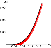
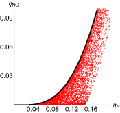
Figure 1: Nonlinearity measures for a weakly perturbed harmonic potential. In the left panel we show $\eta_{\scriptscriptstyle N\!G}[V]$ as a function of $\eta_{\scriptscriptstyle B}[V]$ for random values of $\epsilon_{3}\in[-0.1,0.1]$ and $\epsilon_{4}\in[-0.25,0.25]$. The right panel shows the corresponding values for $\epsilon_{3}\in[-0.2,0.2]$, $\epsilon_{4}\in[-0.25,0.25]$. The solid black line in both plots is the function $\eta_{\scriptscriptstyle N\!G}(\eta_{\scriptscriptstyle B})$ of Eq. (13).

If the nonlinearity is induced by an anharmonic potential that is an even function at lowest orders, i.e. corresponds to $\epsilon_{3}=0$, then we have $\alpha_{1}=0$ and the two measures are monotone of each other, and thus equivalent in assessing the nonlinearity. More precisely, upon inserting Eq. (11) in the expressions of $\eta_{\scriptscriptstyle B}$ and $\eta_{\scriptscriptstyle N\!G}$, we have

$$\eta_{\scriptscriptstyle N\!G}=h\left(\frac{1}{2}\sqrt{1+24\eta_{\scriptscriptstyle B}^{2}(\eta_{\scriptscriptstyle B}^{2}-2)}\right)\,.$$ (13)

On the other hand, if the anharmonic potential contains odd terms, then monotonicity is no longer ensured and should be checked for each specific case. This behavior is illustrated in Fig. 1 where we show parametric plots of $\eta_{\scriptscriptstyle N\!G}$ as a function of $\eta_{\scriptscriptstyle B}$ for potentials corresponding to random values of the parameters $\epsilon_{3}$ and $\epsilon_{4}$. In both panels the solid black curve is the function $\eta_{\scriptscriptstyle N\!G}(\eta_{\scriptscriptstyle B})$ reported in Eq. (13). In the left panel, the red points correspond to random values of $\epsilon_{3}\in[-0.1,0.1]$ and $\epsilon_{4}\in[-0.25,0.25]$, whereas in the right panel we show the corresponding values of $\epsilon_{3}\in[-0.2,0.2]$ and $\epsilon_{4}\in[-0.25,0.25]$.

The general perturbative expansion reported above illustrates that a potential function may deviate from the harmonic behavior in many different ways and ”directions” since, loosely speaking, the space of potential functions is infinite dimensional (and this is true even restricting attention to the ring of polynomials). As a consequence, one would in principle expect that the nonlinearity of an oscillator needs a set of parameters to be characterized. On the other hand, as we will see in the next Section, we prove that for a set of relevant potentials our measure is indeed capturing and quantifying the intuitive notion of nonlinearity, including also cases where the nonlinearity is strong.

III Examples and discussion

In this section we evaluate the nonlinearity of some quantum oscillators subject to potentials chosen on the basis of their relevance, properties, and analytic solvability. We employ the results to compare the behavior of the two measures, and to validate the use of $\eta_{\scriptscriptstyle N\!G}$. We consider only position-dependent potentials $V(x)$, and confine our investigation to the one-dimensional case, where, assuming $m=1$ and $\hbar=1$, the Schrödinger equation reads

$$\left[-\frac{1}{2}\frac{d^{2}}{dx^{2}}+V(x)\right]\phi(x)=E\,\phi(x)\,.$$ (14)

In the following, we are going to address in some detail the nonlinearity of the Morse (M) potential mor29 , $V_{\scriptscriptstyle M}(x)$, the modified Pöschl-Teller (MPT) potential nie78 , $V_{\scriptscriptstyle P}(x)$, the modified isotonic oscillator (MIO) potential car08 , $V_{\scriptscriptstyle T}(x)$, and the Fellows-Smith supersymmetric partner of the harmonic oscillator fs11 $V_{\scriptscriptstyle F}(x)$. These potentials describe a wide range of different physical systems, with striking different physical properties. A common feature, though, is that the eigenfunctions depend explicitly on a parameter that couples the range of the potential and the depth of the well. For the Morse and the MPT potential, this parameter sets also the number of bound states.

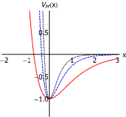
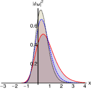
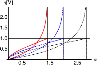
Figure 2: The Morse potential. In the upper left panel we show $V_{\scriptscriptstyle M}(x)$ for $\alpha=1$ (solid red), $\alpha=2$ (dashed blue), $\alpha=3$ (dotted black) and for a fixed depth parameter $D=1$. In the upper right panel we show the corresponding GS probability densities, $|\phi_{\scriptscriptstyle M}|^{2}(x)$. In the lower panel we show the nonlinearity measures $\eta_{\scriptscriptstyle N\!G}\left[\text{V}\right]$ and $\eta_{\scriptscriptstyle B}\left[\text{V}\right]$ as a functions of $\alpha$ for different values of $D$. We have $D=0.25$ (solid red), $D=0.5$ (dashed blue), $D=1$ (dotted black). The vertical black lines are placed in correspondence of the limiting values of $\alpha$.

III.1 The Morse potential

The Morse potential was first suggested by Morse mor29 as an anharmonic potential to describe covalent molecular bonding. It is an asymmetric potential and its expression reads as follows

$$V_{\scriptscriptstyle M}(x)=D(e^{-2\alpha x}-2e^{-\alpha x})\,,$$ (15)

where the coordinate $x$ corresponds to the distance from the minimum of the potential. The coefficient $D>0$ represents the bond dissociation energy, whereas the parameter $\alpha$ controls the width and skewness of the well. Indeed, the eigenvalues of the Morse potential matches very well the experimental spectral lines for the vibration of the nuclei in diatomic molecules. The harmonic limit at fixed $D$ is achieved for $\alpha\rightarrow 0$, whereas the reference harmonic potential corresponds to a frequency $\omega_{\scriptscriptstyle R}=\sqrt{2D}\alpha$. The form of the potential is illustrated in Fig. 2 for different values of $\alpha$. The number of bound states is finite, and is given by the integer part of $N=-\frac{1}{2}+\sqrt{2D}/\alpha$. We thus have the constraint $\alpha<2\sqrt{2D}$ on the parameters in order to have at a least one bound state. For vanishing $D$ or for $\alpha$ approaching $2\sqrt{2D}$ there is just one bound state, the GS. The GS wavefunction is given by

$$\phi_{\scriptscriptstyle M}(x)= \sqrt{2}(2N+1)^{N}\sqrt{\frac{N\alpha}{2N!}}e^{-\alpha xN-(N+\tfrac{1}{2})e^{-\alpha x}}$$ (16)

and corresponds to a bound state with energy $E_{\scriptscriptstyle M}=-\frac{1}{2}\alpha N^{2}$.

After looking at the shape of the potential in Fig. 2, one would expect that the nonlinearity vanishes for $\alpha\rightarrow 0$, and increases with $\alpha$ at any fixed value of $D$. Indeed, this intuitive behavior is captured by both measures, $\eta_{\scriptscriptstyle N\!G}\left[\hbox{V}\right]$ and $\eta_{\scriptscriptstyle B}\left[\hbox{V}\right]$, as they grow continuously and smoothly from zero to the maximum value of $\alpha$ for which the condition on the existence of bound states is fulfilled. The nG-based nonlinearity $\eta_{\scriptscriptstyle N\!G}[V]$ diverges as $\eta_{\scriptscriptstyle N\!G}[V]\simeq 1+\frac{1}{4}\log(D/4)+\frac{1}{2}\log(\alpha-2\sqrt{2D})$ for $\alpha$ approaching $2\sqrt{2D}$ and vanishes as $\eta_{\scriptscriptstyle N\!G}[V]\simeq y(1-\log y)$, where $y=\alpha/16\sqrt{2D}$, for vanishing $\alpha$. At fixed value of $\alpha$ both measures of nonlinearity decrease with increasing $D$, a behavior that correctly captures the shape of the potential (which indeed appears more harmonic when becoming deeper at fixed width).

III.2 The modified Pöschl-Teller potential

The modified Pöschl-Teller potential (MPT) describes several types of diatomic molecules bonding. It also appears in the solitary wave solutions of the Konteweg-de Vries equation, and finds application in the analysis of confined systems as quantum dots and quantum wells. The modified Pöschl-Teller potential nie78 is an even function, given by

$$V_{\scriptscriptstyle P}(x)=-\frac{D}{\cosh^{2}(\alpha x)}\,,$$ (17)

where $D>0$ is the potential depth and $\alpha$ is connected to the range of the potential. As it will be apparent in the following, it is convenient to reparametrize the potential expressing the depth parameter as $D=\frac{1}{2}\alpha^{2}s(1+s)$, where

$$s=\frac{1}{2}(-1+\sqrt{1+8D/\alpha^{2}})>0\,.$$

The harmonic limit for any fixed value of $D$ is obtained for $\alpha\rightarrow 0$, whereas the reference harmonic potential corresponds to a frequency $\omega_{\scriptscriptstyle R}=\sqrt{2D}\alpha=\sqrt{s(s+1)}\alpha^{2}$. The form of the potential is illustrated in the upper left panel of Fig. 3, where $V_{\scriptscriptstyle P}(x)$ is shown for $D=1$ and different values of $\alpha$. The MPT potential is an even function and thus, according to the arguments of the previous Section, we expect the two measures to be monotone functions of each other, at least for small values of $\alpha$. The wavefunction of the ground state is given by

$$\phi{\scriptscriptstyle P}(x)=\frac{1}{\pi^{\frac{1}{4}}}\sqrt{\frac{\alpha\,\Gamma[\frac{1}{2}+s]}{\Gamma[s]}}\frac{1}{\cosh^{s}(\alpha x)}\,,$$ (18)

where $\Gamma[x]$ denotes the Gamma function, and correspond to a bound state with energy $E_{\scriptscriptstyle P}=-\frac{1}{2}\alpha^{2}s^{2}$. The corresponding probability density $|\phi_{\scriptscriptstyle P}(x)|^{2}$ is shown in the upper right panel of Fig. 3 for different values of $\alpha$.

In the lower panel of Fig. 3 we show the two nonlinearity measures as functions of $\alpha$, for $D=1/2$ (red solid line), $D=1$ (blue dashed), $D=3$ (black dotted). Both measures increase monotonically with $\alpha$ and decrease with $D$. The two measures are anyway monotone of each other independently on the value of $D$. This is illustrated in the inset of the lower panel, where we show a parametric plot of $\eta_{\scriptscriptstyle B}$ as a function of $\eta_{\scriptscriptstyle N\!G}$. The plot has been obtained by varying $\alpha$ at fixed values of $D$ (the same values used above). As it is apparent from the plot, the three curves superimpose each other.

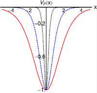
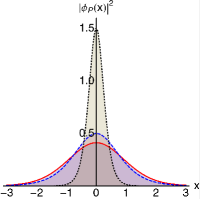
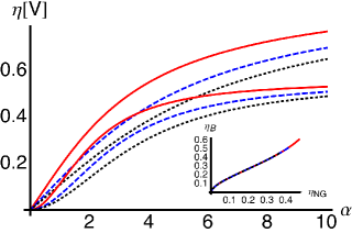
Figure 3: The modified Pöschl-Teller potential. The upper panels show the MPT potential $V_{\scriptscriptstyle P}(x)$ and the corresponding ground state probability density $|\phi_{\scriptscriptstyle P}(x)|^{2}$ for $\alpha=1/2$ (solid red lines), $\alpha=1$ (blue dashed) and $\alpha=3$ (black dotted) and a fixed potential depth $D=1$. In the lower panel we show the nonlinearity measures $\eta_{\scriptscriptstyle B}[V_{\scriptscriptstyle P}]$ and $\eta_{\scriptscriptstyle N\!G}[V_{\scriptscriptstyle P}]$ as a function of $\alpha$ for $D=1$ (red solid line), $D=2$ (blue dashed), $D=3$ (black dotted). The inset is a parametric plot of $\eta_{\scriptscriptstyle B}$ as a function of $\eta_{\scriptscriptstyle N\!G}$, showing that the two measures are monotone functions of each other, independently on the value of $D$.

III.3 The modified isotonic potential

The so-called isotonic oscillator is a quantum system subjected to a potential of the form $V(x)\propto\omega^{2}x^{2}+g/x^{2}$ with $g>0$. Roughly speaking, the potential is aimed to describe harmonic oscillators in the presence of a barrier. The isotonic oscillator has an equally spaced spectrum and it is exactly solvable. The potential of the so-called modified isotonic oscillator (MIO) car08 ; yes11 is given by

$$V_{\scriptscriptstyle T}(x)=\frac{1}{2}\left[x^{2}+4\frac{(a+2)(ax^{2}-1)}{a(ax^{2}+1)^{2}}\right]\qquad a>0\,.$$ (19)

The MIO class describes a family of oscillators which interpolate between the harmonic and the isotonic oscillator, and represents a good testbed for a measure of nonlinearity. We have $V_{\scriptscriptstyle T}(x)\simeq-D+\frac{1}{2}\omega_{\scriptscriptstyle R}^{2}x^{2}$ for small values of $x$, where the depth of the potential is given by $D=2(a+2)/a$ and the reference frequency by $\omega_{\scriptscriptstyle R}=\sqrt{25+12a}$, whereas for large $x$ the potential approaches $V_{\scriptscriptstyle T}(x)\simeq\frac{1}{2}x^{2}+D/(ax^{2})$. The form of the potential for different values of $a$ is shown in the left panel of Fig. 4. The ground state has energy $E_{\scriptscriptstyle T}=\frac{1}{2}-\frac{4}{a}$ and the corresponding wavefunction is given by

$$\phi_{\scriptscriptstyle T}(x)=\frac{1}{\pi^{\frac{1}{4}}\sqrt{\Phi(\frac{4}{a},\frac{1}{2}+\frac{4}{a};\frac{1}{a})}}\,e^{-\frac{1}{2}x^{2}}\left(\frac{1}{a}+x^{2}\right)^{-\frac{2}{a}}\,,$$

where $\Phi(a,b;z)$ is the confluent hypergeometric function. As the form of the potential may suggest, oscillators subjected to MIO potentials have the ground state detached from the rest of the eigenstates, which are equally spaced in energy. The GS probability densities, $|\phi_{\scriptscriptstyle T}|^{2}(x)$ is shown in the upper right panel of Fig. 4.

We have evaluated the nonlinearity measures as a function of the parameter $a$ and the results are reported in the lower panel of Fig. 4. As it is apparent from the plot, the two measures are monotone of each other, and may be used equivalently, as far as the value of $a$ is not too large. For increasing $a$ the Bures measure continue to grow whereas $\eta_{\scriptscriptstyle N\!G}$ has a maximum and then starts to decrease, thus no longer representing a suitable quantity to assess the nonlinear features of $V_{\scriptscriptstyle T}$. This behavior is due to the peculiar structure of the eigenstates: Indeed the ground state of the system, though departing from that of the harmonic reference, is becoming more and more Gaussian, thus resembling that of a harmonic oscillator (not the reference one). In fact, the nonlinear features of the potential are encoded in the rest of the eigenstates. In order to capture the nonlinear features of this kind of potentials, we have to use $\eta_{\scriptscriptstyle B}$ or to look at the non-Gaussian properties of states at thermal equilibrium, which account for the whole spectrum.

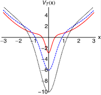
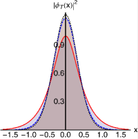
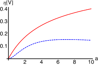
Figure 4: The modified isotonic potential. The upper left panel shows the MIO potential $V_{\scriptscriptstyle T}(x)$ for different values of the parameter: $a=5$ (solid red), $a=1$ (blue dashed) and $a=\frac{1}{2}$ (black dotted). The upper right panel shows the probability density $|\phi_{\scriptscriptstyle T}(x)|^{2}$ of the corresponding GS wavefunctions. In the lower panel we show the nonlinearity measures $\eta_{\scriptscriptstyle B}\left[\text{V}\right]$ (solid red line) and $\eta_{\scriptscriptstyle N\!G}\left[\text{V}\right]$ (dashed blue) as a function of $a$.

III.4 The Fellows-Smith potential

We end this Section by considering a set of nonlinear oscillators corresponding to a class of potentials which have no clear harmonic reference, such that the Bures measure of nonlinearity cannot be properly defined. These correspond to a class of supersimmetric partners of the harmonic potential, given by fs11

$$V_{\scriptscriptstyle F}(x) =-2p+\frac{1}{2}x^{2}+4\,(1+p)\,x^{2}\frac{\Phi(\frac{3+p}{2},\frac{3}{2};x^{2})}{\Phi(\frac{1+p}{2},\frac{1}{2};x^{2})^{2}}$$

$$\times \left[(1+p)\,\Phi(\frac{3+p}{2},\frac{3}{2};x^{2})-\Phi(\frac{1+p}{2},\frac{1}{2};x^{2})\right]\,,$$ (20)

where $\Phi(a,b;z)$ is the confluent hypergeometric function and $p\in(-1,0]$. The potentials show a single well structure for $p\in[p_{+},0]$, a double well structure for $p\in[p_{-},p_{+}]$ and a triple one for $p\in[-1,p_{-}]$, where $p_{\pm}=-\frac{1}{2}\pm\frac{\sqrt{2}}{4}$. The behavior of $V_{\scriptscriptstyle F}(x)$ in the different regions is illustrated in the upper left panel of Fig. 5, where we show the potentials for $p=-\frac{1}{10},-\frac{3}{5},-\frac{9}{10}$ respectively. The corresponding probability distributions of the ground state $|\phi_{\scriptscriptstyle F}(x)|^{2}$ are shown in the upper right panel of the same figure. The wave function of the ground state is given by

$$\phi_{\scriptscriptstyle F}(x)=\frac{1}{\pi^{\frac{1}{4}}}\,\sqrt{\frac{2^{p}}{\Gamma[1+p]}}\,\frac{\Gamma[1+\frac{p}{2}]\,e^{\frac{1}{2}x^{2}}}{\Phi(\frac{1+p}{2},\frac{1}{2};x^{2})}\,,$$

and corresponds to the eigenvalue $E_{\scriptscriptstyle F}=\frac{1}{2}-p$.

As it is apparent from the plot and from the structure of the potential, it is possible to define a proper reference harmonic oscillator only for $p\in[p_{+},0]$: in this case we have $\omega_{\scriptscriptstyle R}=\sqrt{1+8p(1+p)}$, which is vanishing for $p\rightarrow p_{\pm}$. For $p\in[p_{-},p_{+}]$ there is no such option, unless one breaks the symmetry of the potential and arbitrarily choose one of the two minima to define a reference harmonic oscillator. In the third region, $p\in(-1,p_{-}]$, the potential shows again a mininum at $x=0$. However, using this feature to define the reference harmonic potential is obviously misleading, since it ignores the main features of the potential.

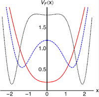
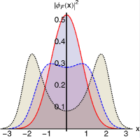
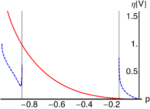
Figure 5: The Fellows-Smith potential. The upper left panel shows $V_{\scriptscriptstyle F}(x)$ for different values of the parameter: $p=-\frac{1}{10}$ (solid red), $p=-\frac{2}{5}$ (blue dashed) and $p=-\frac{9}{10}$ (black dotted). The upper right panel shows the probability density $|\phi_{\scriptscriptstyle F}(x)|^{2}$ of the corresponding GS wavefunctions. In the lower panel we show the nonlinearity measure $\eta_{\scriptscriptstyle N\!G}\left[\text{V}\right]$ (solid red line) as a function of $p$, together with the measure $\eta_{\scriptscriptstyle B}\left[\text{V}\right]$ (dashed blue) in the regions where it can be evaluated. The vertical black lines denote the values $p=p_{\pm}$.

We have evaluated the nonlinearity measure $\eta_{\scriptscriptstyle N\!G}$ for $p\in(-1,0]$ and the Bures one $\eta_{\scriptscriptstyle B}$ where it is possible. Results are shown in the lower panel of Fig. 5, where the solid red line and the blue dashed one denote respectively $\eta_{\scriptscriptstyle N\!G}$ and $\eta_{\scriptscriptstyle B}$. As it is apparent from the plot, $\eta_{\scriptscriptstyle N\!G}$ monotonically decreases with $p$, thus properly capturing the nonlinear behavior of the $V_{\scriptscriptstyle F}$ potential. Besides, the two measures are monotone of each other for $p\in[p_{+},0]$, where the Bures measures may be properly defined. The plot also makes apparent that despite $\eta_{\scriptscriptstyle B}$ may be calculated also for $p\in(-1,p_{-}]$, its behavior is not consistent with the behavior at smaller values of $p$, thus failing to provide a quantitative assessment of nonlinearity. In particular, $\delta_{\scriptscriptstyle B}\rightarrow 1$ for $p\rightarrow p_{-}$, then, as $p$ decreases, it shows a minimum and then starts to increase for $p$ that decreases to $p=-1$.

IV Conclusions

Quantum oscillators with nonlinear behavior induced by anharmonic potentials have attracted interest in different fields, as they play a relevant role for fundamental and practical purposes. In particular, they have recently received attention as a possible resource for quantum technology and information processing. As a consequence, it would be useful to have a suitable measures of nonlinearity to better characterize these potentials and to better assess their performances in those fields. In this paper, we have addressed the quantification of nonlinearity for quantum oscillators, and have introduced two measures of nonlinearity based on the properties of the ground state of the potential, rather than on the form of the potential itself. The first measure accounts for the Bures distance between the potential GS and that of a reference harmonic potential. It is a natural choice for a measure of nonlinearity, however it requires the knowledge of the potential near its minimum. We have thus suggested a different measure, based on the non-Gaussian properties of the potential GS, which may be calculated using only information about the GS itself.

The two measures have been analyzed and compared, both in terms of their general properties and by evaluating them for some significant anharmonic potentials. Our results show that the nG-based measure has some merits which makes it a good choice for the purpose of assessing nonlinearity. In fact, while it captures the nonlinear features of oscillators as the Bures measures in most cases (e.g., for any anharmonic potential which is an even function at lowest orders) it has a clear advantage from a computational and experimental point of view: it does not require the determination of a reference frequency and thus it does not need any a priori information on the corresponding potential to be calculated. The only ingredient needed to evaluate $\eta_{\scriptscriptstyle N\!G}$ is the GS wavefunction, a task that can be pursued by tomographic reconstruction independently on the specific features of the potential. In addition, we have seen examples of potentials where the Bures measure cannot be defined, due to the lack of a proper reference harmonic potential, whereas the nG-based properly quantify the nonlinear features of the oscillator behavior. Moreover, from a more fundamental point of view, the validity of the measure $\eta_{\scriptscriptstyle N\!G}$ is strengthened by the fact that the same amount of non-linearity is assigned to non-linear Hamiltonians which are related by symplectic transformation in phase-space (displacement, phase-rotation and squeezing), inducing a reasonable and expected hierarchy.

Overall, we have addressed the general issue of assessing the nonlinearity of a quantum potential, highlighted the current limits, and nevertheless individuated a consistent method to quantify the nonlinearity based on non-Gaussianity of the potential’s ground state. In order to fully validate the measure(s) here proposed we would have needed an already established way to compare nonlinear potentials and assess their diversity. Then we could have tried to prove some form of continuity of our measure(s) with respect this quantity .Not having a measure or a set of criteria of this kind is among the motivations of our work while being able to summarize the nonlinear character by a single quantity is the main result.

Finally, we notice that our results could be exploited in any experiments, e.g., on quantum control, where either by technological of fundamental issues, information on the confining potential in inaccessible or limited. Our approach may be generalized and refined by taking into account the non-Gaussian features of the Gibbs thermal states of the nonlinear oscillators, rather than the sole GS.

Appendix A Gaussian states

The density operator of a single-mode continuous-variable state $\rho$ can be fully represented by its characteristic function,

$$\chi[\rho](\mathbf{\lambda})=\hbox{Tr}[\rho D(\lambda)],$$ (21)

where $\lambda$ is a complex number and $D(\lambda)$ is the displacement operator $D(\lambda)=e^{\lambda a^{\dagger}-\lambda^{*}a}$. Equivalently, we may describe the quantum state using its Wigner function, which is the Fourier transform of the characteristic function

$$W[\rho](z)=\int\frac{\hbox{d}\lambda^{2}}{\pi^{2}}\,e^{\lambda^{*}z-\lambda z^{*}}\,\chi[\rho](\lambda)\,.$$ (22)

A quantum state is said to be Gaussian if its characteristic function (and thus also the Wigner function) is Gaussian. Before writing the expression explicitly, we must introduce the vector of mean values $\bar{X}$ and the covariance matrix $\sigma$, with elements

$$\bar{X}_{k} =\langle R_{k}\rangle$$

$$\sigma_{jk} =\frac{1}{2}\langle\{R_{j},R_{k}\}\rangle-\langle R_{j}\rangle\langle R_{k}\rangle\,,$$ (23)

where $R=(x,p)$, $\{A,B\}=AB+BA$, and $\langle A\rangle=\hbox{Tr}\left[\rho A\right]$. The Wigner function of a Gaussian state $\rho_{G}$ is equal to

$$W[\rho_{G}](X)=\frac{1}{2\pi\sqrt{\hbox{det}[\sigma]}}\hbox{exp}\left[-\frac{1}{2}(X-\bar{X})^{T}\sigma^{-1}(X-\bar{X})\right]$$ (24)

where $X=(\hbox{Re}\,z,\hbox{Im}\,z)$. Gibbs thermal states and ground states of Hamiltonians that are at most bilinear in the mode operators are Gaussian states, the harmonic oscillator being a paradigmatic example.

References

- (1) J. K. Bhattacharjee, A. K. Mallik, S.Chakraborty, Ind. J. Phys. 81, 1115 (2007).
- (2) V. Perinova, A. Luks, Progr. Opt. 33, 129 (1994).
- (3) A. Nunnenkamp, Phys. Rev. Lett. 107, 063602 (2011).
- (4) J. Eisert, M. B. Plenio, Int. J. Quant. Inf. 1, 479 (2003).
- (5) A. Ferraro, S. Olivares and M. G. A. Paris, Gaussian States in Quantum Information, (Bibliopolis, Napoli, 2005).
- (6) S. Olivares, Eur. Phys. J. ST 203, 3 (2012).
- (7) C. Weedbrook, S. Pirandola, R. Garcia-Patron, N. J. Cerf, T. C. Ralph, J. H. Shapiro, S. Lloyd, Rev. Mod. Phys. 84, 621 (2012).
- (8) M. G. Genoni, M. G. A. Paris, K. Banaszek, Phys. Rev. A 76 , 042327 (2007).
- (9) M. G. Genoni, M. G. A. Paris, K. Banaszek, Phys. Rev. A 78 , 060303(R) (2008).
- (10) M. G. Genoni, M. G. A. Paris, Phys. Rev. A 82, 052341 (2010).
- (11) P. Marian, T. A. Marian, Phys. Rev. A 88, 012322 (2013).
- (12) J. Eisert, S. Scheel, and M. B. Plenio, Phys. Rev. Lett. 89, 137903 (2002).
- (13) G. Giedke and J. I. Cirac, Phys. Rev. A 66, 032316 (2002).
- (14) J. Fiurasek, Phys. Rev. Lett. 89, 137904 (2002).
- (15) M. G. Genoni, P. Giorda, M. G. A. Paris J. Phys. A 44, 152001 (2011).
- (16) J. Niset, J. Fiurasek and N. J. Cerf, Phys. Rev. Lett. 102, 120501 (2009).
- (17) E. T. Owen, M. C. Dean, and C. H. W. Barnes, Phys. Rev. A 85, 022319 (2012).
- (18) C. Vierheilig, F. Bercioux, M. Grifoni, Phys. Rev. A 83, 012106 (2011).
- (19) G. M. D’Ariano, L. Maccone, M. G. A. Paris, J. Phys. A, 34, 93 (2001).
- (20) P. M. Morse, Phys. Rev. 34, 57 (1929).
- (21) M. N. Nieto, Phys. Rev. A 17, 1273 (1978).
- (22) J. F. Cariñena, A. M. Perelomov, M. F. Rañada, M. Santander J. Phys. A 41, 085301 (2008)
- (23) Ö. Yesiltas, J. Phys. A 44, 305305 (2011).
- (24) J. M. Fellows, R. A. Smith, J. Phys. A 44, 335302 (2011).