Anytime Control using Input Sequences with Markovian Processor Availability

Abstract

We study an anytime control algorithm for situations where the processing resources available for control are time-varying in an a priori unknown fashion. Thus, at times, processing resources are insufficient to calculate control inputs. To address this issue, the algorithm calculates sequences of tentative future control inputs whenever possible, which are then buffered for possible future use. We assume that the processor availability is correlated so that the number of control inputs calculated at any time step is described by a Markov chain. Using a Lyapunov function based approach we derive sufficient conditions for stochastic stability of the closed loop.

I Introduction

Recently, many works have appeared that consider the impact of limited or time-varying processing power on control algorithms. Such problems arise naturally in cyberphysical and embedded systems where the control algorithm may be just one of many tasks being executed by the processor. Thus, McGovern and Feron [10, 11] considered the question of bounding the processing time that is required to solve the optimization problem in model predictive control to a specified accuracy. Henriksson et al [5, 6] studied the trade-off inherent in solving the optimization problem exactly (thus, obtaining the control input sequence more precisely) and in solving the problem more often. Event-triggered and self-triggered control, and online sampling, e.g., [17, 19, 18, 2] have also been proposed as a means to ensure less demand on the processor on average by calculating the control input on demand in a non-periodic fashion.

In this note, we are interested in anytime control algorithms. Such algorithms calculate a coarse control input even with limited processing resources. As more processing resources become available, the input is refined. The process can be terminated at any time by the processor. The quality of control input is thus time-varying, but no control input is obtained only rarely. Various anytime algorithms for linear processors and controllers have been proposed in the literature [1, 3, 4]. For non-linear plants, we recently proposed anytime algorithms based on computing sequences of potential (tentative) future control values [15]. At the instances when more processing power is available, a longer sequence is calculated. This provides a buffer against the time steps when the processor power is not enough to calculate an input. Since the control values in the sequence are calculated by reutilising already computed values, the algorithm does not assume a priori knowledge of processor availability.

However, with the exception of [3] and [15], the analysis in these works largely considered the processor availability to be described by an independent and identically distributed sequence. In particular, [15] had a brief discussion when the processor availability sequence is described by a (hidden) Markov chain; the memory arose through the concept of ‘processor states’ which are not directly related to how many control values can be calculated. In the current work, we replace this model by a more direct one, where the processor availability for the control task, and hence the number of tentative control values that can be calculated at each time step, forms a Markov Chain. More importantly, we provide a new analysis technique, that at least for a class of models, is less conservative than the technique in [15]. Intuitively, the proposed technique considers the ‘average’ case of processor availability to analyze a random-time drift condition, as compared to the ‘worst case’ analysis in [15]. Sufficient conditions for stochastic stability with and without the anytime control algorithm are provided and compared with the conditions in [15]. We also analyze the robustness of these conditions with respect to presence of process noise. A preliminary version of parts of the present manuscript can be found in [14].

The paper is organized as follows: In Section II, we present the control design problem studied. In Section III, we revise the anytime algorithm of[15] to be studied. Section IV presents a novel model for analyzing the resulting closed loop when the processor availability is Markovian. Section V presents the stability analysis with this model. Section VI compares our results with those in[15]. Section VII provides robust stability analysis in the presence of process noise. Numerical simulations are documented in Section VIII. Section IX draws conclusions.

Notation

We write $\mathbb{N}$ for $\{1,2,3,\ldots\}$, $\mathbb{N}_{0}$ for $\mathbb{N}\cup\{0\}$ and $\mathbb{N}_{n}^{m}=\{n,n+1,\ldots,m\},$ for given integers $n\leq m$. $\mathbb{R}$ are the real numbers and $\mathbb{R}_{\geq 0}$ the nonnegative real numbers. The $p\times p$ identity matrix is denoted by $I_{p}$ and the $p\times q$ matrix of all ones is denoted by $I_{p\times q}$, whereas $0_{p}=0I_{p}$ and $\mathbf{0}_{p}$ is the all-zeroes (column) vector in $\mathbb{R}^{p}$. The notation $\{x\}_{\mathcal{K}}$ stands for $\{x(k)\;\colon k\in\mathcal{K}\}$. We adopt the convention $\sum_{k=\ell_{1}}^{\ell_{2}}a_{k}=0$ if $\ell_{1}>\ell_{2}$ and irrespective of $a_{k}\in\mathbb{R}$. The superscript ^T refers to transpose. The Euclidean norm of a vector $x$ is denoted by $|x|=\sqrt{x^{T}x}$. A function $\varphi\colon\mathbb{R}_{\geq 0}\to\mathbb{R}_{\geq 0}$ is of class-$\mathscr{K}_{\infty}$ ($\varphi\in\mathscr{K}_{\infty}$), if it is continuous, zero at zero, strictly increasing, and unbounded. The probability of event $\Omega$ is $\mathbf{Pr}\{\Omega\}$ and the conditional probability of $\Omega$ given $\Gamma$ is $\mathbf{Pr}\{\Omega\,|\,\Gamma\}$. The expected value of $\nu$ given $\Gamma$, is denoted by $\mathbf{E}\{\nu\,|\,\Gamma\}$; for the unconditional expectation we write $\mathbf{E}\{\nu\}$. An $m\times n$ matrix $M$ whose $(i,j)$-th element is $m_{ij}$ is denoted by $M=\left[m_{ij}\right]_{m\times n}$.

II Control with Random Processor Availability

Consider a discrete-time non-linear plant that evolves as

$$x(k+1)=f(x(k),u(k)),\quad k\in\mathbb{N}_{0},$$ (1)

where the state $x(.)\in\mathbb{R}^{n}$ and the control input $u(.)\in\mathbb{R}^{p}.$ We assume that the origin is an equilibrium point of the plant, so that $f(\mathbf{0}_{n},\mathbf{0}_{p})=\mathbf{0}_{n}$. The initial state $x(0)$ is arbitrary. Given the stochastic processor availability model that we assume (as described below), the plant can evolve in open loop for arbitrarily long times. For general non-linear plants, the state may thus assume a value such that no possible control sequence can stabilize the process. To prevent this eventuality, we assume that (1) is globally controllable via state feedback.

Assumption 1

There exist functions $V\colon\mathbb{R}^{n}\to\mathbb{R}_{\geq 0}$, $\varphi_{1},\varphi_{2}\in\mathscr{K}_{\infty}$, a constant $\rho\in[0,1)$, and a control policy $\kappa\colon\mathbb{R}^{n}\to\mathbb{R}^{p}$, such that for all $x\in\mathbb{R}^{n},$

$$\begin{split}\varphi_{1}(|x|)\leq V(x)&\leq\varphi_{2}(|x|),\\ V(f(x,\kappa(x)))&\leq\rho V(x).\end{split}$$ (2)

If the plant (1) is considered to be obtained by sampling a continuous-time plant, it is generally assumed that the control calculation can be completed within a fixed (and small) time-delay, say $\delta\in(0,T_{s})$. However, in networked and embedded systems, the processing resources (e.g., processor execution times) for control may vary, and, at times, be insufficient to generate a control input within the prescribed timeout $\delta$. This can lead to instances where the plant evolves uncontrolled, even though there was an excess of processing resource availability (beyond what is required to calculate a single control input) at other time instants. The anytime control algorithm we propose makes better use of this excess availability to safeguard against the time steps at which the processing resource was not available at all.

Before describing the anytime algorithm, we discuss a baseline algorithm that arises from a direct implementation of the control policy $\kappa$ used in Assumption 1. In this algorithm, the plant input which is applied during the interval $[kT_{s}+\delta,(k+1)T_{s}+\delta)$ is given by

$$u(k)=\begin{cases}\kappa(x(k))&\text{if sufficient computational resources to evaluate $\kappa(x(k))$ are available}\\ &\text{between times $kT_{s}$ and $kT_{s}+\delta$,}\\ \mathbf{0}_{p}&\text{otherwise.}\end{cases}$$ (3)

We shall assume that the controller requires processor time to carry out mathematical computations. However, simple operations at a bit level, such as writing data into buffers, shifting buffer contents and setting values to zero do not require processor time. Similarly, input-output operations, i.e., A/D and D/A conversion are triggered by external asynchronous loops with a real-time clock and do not require that the processor be available for control. As in regular discrete-time control, these external loops ensure that state measurements are available at the instants $\{kT_{s}\}_{k\in\mathbb{N}_{0}}$ and that the controller outputs (if available) are passed on to the plant actuators at times $\{kT_{s}+\delta\}_{k\in\mathbb{N}_{0}}$, where $\delta$ is fixed.

III Sequence-based Anytime Control Algorithm

We use the same anytime control algorithm as proposed in [15] that calculates and buffers a sequence of tentative future plant inputs at time intervals when the controller is provided with more processing resources than are needed to evaluate the current control input. Denote the buffer states via $\{b\}_{\mathbb{N}_{0}}$, where

$$b(k)=\left[\begin{array}[]{lcr}b_{1}^{T}(k)&\cdots&b_{\Lambda}^{T}(k)\end{array}\right]^{T}\in\mathbb{R}^{\Lambda p},\quad k\in\mathbb{N}_{0},$$

for a given value $\Lambda\in\{2,3,\dots\}$ and where each $b_{j}(k)\in\mathbb{R}^{p}$, $j\in\mathbb{N}_{1}^{\Lambda}$. Also define a shift matrix

$$S\triangleq\begin{bmatrix}0_{p}&I_{p}&0_{p}&{1}&0_{p}\\ \vdots&\ddots&\ddots&\ddots&\vdots\\ 0_{p}&\dots&0_{p}&I_{p}&0_{p}\\ 0_{p}&{2}&0_{p}&I_{p}\\ 0_{p}&{3}&0_{p}\end{bmatrix}\in\mathbb{R}^{\Lambda p\times\Lambda p}.$$

Fig. 1 presents the algorithm, which we denote by A₁.

 

Step 1

: At time $t=0$,

set $b(-1)\leftarrow\mathbf{0}_{\Lambda p}$, $k\leftarrow 0$;

Step 2

: if $t\geq kT_{s}$, then

input $x(k)$;

set $\chi\leftarrow x(k)$, $j\leftarrow 1$, $b(k)\leftarrow Sb(k-1)$;

end

Step 3

: while “sufficient processor time is available” and time $t<(k+1)T_{s}$ and $j\leq\Lambda$,

evaluate $u_{j}(k)=\kappa(\chi)$;

if $j=1$, then

output $u_{1}(k)$;

set $b(k)\leftarrow\mathbf{0}_{\Lambda p}$;

end

set $b_{j}(k)\leftarrow u_{j}(k)$;

if “sufficient processor time is not available” or $t\geq(k+1)T_{s}$, then

goto Step 5;

end

set $\chi\leftarrow f(\chi,u_{j}(k))$, $j\leftarrow j+1$;

end

Step 4

: if $j=1$, then

output $b_{1}(k)$;

end

Step 5

: set $k\leftarrow k+1$ and goto Step 2;

 

Figure 1: Anytime algorithm A₁, adapted from [15].

Note that the algorithm essentially amounts to a dynamic state feedback policy with internal state variable $b(k)$. Denote by $N(k)\in\mathbb{N}_{0}^{\Lambda}$ the total number of iterations of the while-loop in Step 3 which are carried out during the interval $t\in(kT_{s},(k+1)T_{s})$. This yields:

$$b(k)=\begin{cases}Sb(k-1)&\text{if $N(k)=0$,}\\ \begin{bmatrix}\vec{u}(k)^{T}&(\mathbf{0}_{(\Lambda-N(k))p})^{T}\end{bmatrix}^{T}&\text{if $N(k)\geq 1$,}\end{cases}$$ (4)

where

$$\vec{u}(k)=\begin{bmatrix}u_{1}(k)\\ u_{2}(k)\\ \vdots\\ u_{N(k)}(k)\end{bmatrix}\in\mathbb{R}^{N(k)\cdot p}.$$

The outcomes of the process $\{N\}_{\mathbb{N}_{0}}$ affect the resultant closed loop performance since they determine how many values which stem from the tentative control sequences $\{\vec{u}(k-\ell)\}$, $\ell\in\mathbb{N}_{0}$ are contained in the buffer state $b(k)$. We refer to this quantity as the effective buffer length (at time $k\in\mathbb{N}_{0}$), denote it as $\lambda(k)\in\mathbb{N}_{0}^{\Lambda}$ and note that with initial state $\lambda(-1)=0,$

$$\lambda(k)=\begin{cases}N(k)&\text{if $N(k)\geq 1$},\\ \max(\lambda(k-1)-1,0)&\text{if $N(k)=0$}.\end{cases}$$ (5)

Example III.1

Suppose that $\Lambda=4$ and that the processor availability is such that $N(0)=4$, $N(1)=0$, $N(2)=1$, $N(3)=2$. When using the anytime algorithm A₁, the buffer state at times $k\in\{0,1,2,3\}$ becomes:

$$\{b(0),b(1),b(2),b(3)\}=\left\{\begin{bmatrix}{u_{0}(0)}\\ u_{1}(0)\\ u_{2}(0)\\ u_{3}(0)\end{bmatrix}\!,\begin{bmatrix}{u_{1}(0)}\\ u_{2}(0)\\ u_{3}(0)\\ \mathbf{0}_{p}\end{bmatrix}\!,\begin{bmatrix}{u_{0}(2)}\\ \mathbf{0}_{p}\\ \mathbf{0}_{p}\\ \mathbf{0}_{p}\end{bmatrix}\!,\begin{bmatrix}{u_{0}(3)}\\ u_{1}(3)\\ \mathbf{0}_{p}\\ \mathbf{0}_{p}\end{bmatrix}\right\}$$

which gives $\lambda(0)=4$, $\lambda(1)=3$, $\lambda(2)=1$, $\lambda(3)=2$, and the plant inputs $u(0)=u_{0}(0)$, $u(1)=u_{1}(0)$, $u(2)=u_{0}(2)$, and $u(3)=u_{0}(3)$. On the other hand, if the baseline-algorithm in (3) is used, then $u(0)=\kappa(x(0))$, $u(1)=\mathbf{0}_{p}$, $u(2)=\kappa(x(2))$ and $u(3)=\kappa(x(3))\}$, i.e., at time $k=1$ the plant input is set to zero. This suggests that Algorithm A₁ will outperform the baseline algorithm. $\square$

IV Markov Chain Model and Analysis

In[15] we studied Algorithm A₁ under the assumption that $\{N\}_{\mathbb{N}_{0}}$ is governed by an underlying correlated processor state process. In this work, we examine an alternative model wherein $\{N\}_{\mathbb{N}_{0}}$ is directly described by a finite Markov Chain [9]. As we shall see in Section VI, the current model enables us to develop sufficient conditions for stability, which are less conservative than those in[15].

Assumption 2

The process $\{N\}_{\mathbb{N}_{0}}$ is a homogeneous Markov Chain with initial state $N(0)=0$ and an irreducible and aperiodic transition probability matrix $\mathcal{Q}=[q_{ij}]_{\mathbb{N}_{0}^{\Lambda}\times\mathbb{N}_{0}^{\Lambda}}$ where

$$q_{ij}=\mathbf{Pr}\{N(k+1)=j\,|\,N(k)=i\},\quad i,j\in\mathbb{N}_{0}^{\Lambda}.$$ (6)

The above model allows for correlations in processor availability. Fig. 2 depicts the transition graph for $\{N\}_{\mathbb{N}_{0}}$ resulting from (6) for the case where $\Lambda=2$.

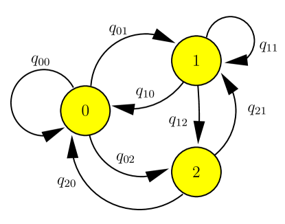
Figure 2: Transition graph of $N$ for $\Lambda=2$.

IV-A Defining an aggregated process

We will analyze the anytime control system through the aggregated process $\{Z\}_{\mathbb{N}_{0}}$, where each

$$Z(k)\triangleq(N(k),\lambda(k)),\quad k\in\mathbb{N}_{0}$$

belongs to the set $\mathbb{S}\triangleq\{s_{0},s_{1},\dots,s_{2\Lambda-1}\}$, having elements $s_{i}=(i,i),\forall i\in\mathbb{N}_{0}^{\Lambda}$ and $s_{\Lambda+j}=(0,j),\forall j\in\mathbb{N}_{1}^{\Lambda-1}.$ Clearly the outcomes of $\{N\}_{\mathbb{N}_{0}}$ determine the trajectory of $\{Z\}_{\mathbb{N}_{0}}$ and thereby determine whether the buffer contains calculated control values or not. An important property is that, if Assumption 2 holds, then $\{Z\}_{\mathbb{N}_{0}}$ is a Markov Chain. The transition probabilities

$$p_{ij}=\mathbf{Pr}\{Z(k+1)=s_{j}\,|\,Z(k)=s_{i}\},\quad(s_{i},s_{j})\in\mathbb{S}\times\mathbb{S}$$

and the associated transition matrix $\mathcal{P}=[p_{ij}],{i,j\in\mathbb{N}_{0}^{2\Lambda-1}},$ are determined by the transition probabilities of $\{N\}_{\mathbb{N}_{0}}$ as detailed in the following lemma:

Lemma IV.1

Suppose that Assumption 2 holds, then

$$\begin{split}&p_{00}=q_{00},\;p_{10}=q_{10},\;p_{(\Lambda+1)0}=q_{00},\\ &p_{ij}=q_{ij},\quad\forall(i,j)\in\mathbb{N}_{0}^{\Lambda}\times\mathbb{N}_{1}^{\Lambda},\\ &p_{(j+1)(\Lambda+j)}=q_{(j+1)0},\quad\forall j\in\mathbb{N}_{1}^{\Lambda-1},\\ &p_{(\Lambda+m)(\Lambda+m-1)}=q_{00},\quad\forall m\in\mathbb{N}_{2}^{\Lambda-1},\\ &p_{(\Lambda+k)l}=q_{0l},\quad\forall(k,l)\in\mathbb{N}_{1}^{\Lambda-1}\times\mathbb{N}_{1}^{\Lambda}.\end{split}$$ (7)

All other transition probabilities in $\mathcal{P}$ are identically zero.

Proof:

See Appendix A. ∎

Example IV.1

Suppose that $\Lambda=3$. Then $\mathbb{S}=\{s_{0},\dots,s_{5}\}$, where $s_{0}=(0,0)$, $s_{1}=(1,1)$, $s_{2}=(2,2)$, $s_{3}=(3,3)$, $s_{4}=(0,1)$, and $s_{5}=(0,2)$. The result (7) then gives:

$$\mathcal{P}=\begin{bmatrix}q_{00}&q_{01}&q_{02}&q_{03}&0&0\\ q_{10}&q_{11}&q_{12}&q_{13}&0&0\\ 0&q_{21}&q_{22}&q_{23}&q_{20}&0\\ 0&q_{31}&q_{32}&q_{33}&0&q_{30}\\ q_{00}&q_{01}&q_{02}&q_{03}&0&0\\ 0&q_{01}&q_{02}&q_{03}&q_{00}&0\end{bmatrix}.$$

IV-B Distribution of the first return time

Denote the times when $b(k)$ runs out of calculated control values, i.e., when $Z(k)=s_{0}=(0,0)$ (equivalently, $\lambda(k)=0$), via $\mathcal{K}=\{k_{i}\}_{i\in\mathbb{N}_{0}}$, where $k_{0}=0$ (from Assumption 2) and

$$k_{i+1}=\inf\big{\{}k\in\mathbb{N}\colon k>k_{i},\quad Z(k)=s_{0}\big{\}},i\in\mathbb{N}_{0}.$$

We also describe the amount of time steps between consecutive elements of $\mathcal{K}$ via $\Delta_{i}\in\mathbb{N}$, where:

$$\Delta_{i}\triangleq k_{i+1}-k_{i},\quad\forall(k_{i+1},k_{i})\in\mathcal{K}\times\mathcal{K}.$$

Thus, the process $\{\Delta_{i}\}_{i\in\mathbb{N}_{0}}$ corresponds to the first return time of state $s_{0}$ and is therefore i.i.d. (see, e.g., [9]). Now the transition matrix of $\{Z\}_{\mathbb{N}_{0}}$ can be partitioned according to (see (7))

$$\begin{split}\mathcal{P}&=\begin{bmatrix}q_{00}&\theta^{T}\\ \mu&\overline{\mathcal{P}}\end{bmatrix},\quad\theta^{T}=\begin{bmatrix}q_{01}&\dots&q_{0\Lambda}&(\mathbf{0}_{\Lambda-1})^{T}\end{bmatrix},\quad\overline{\mathcal{P}}=[p_{ij}],\quad i,j\in\mathbb{N}_{1}^{2\Lambda-1}\\ \mu^{T}&=\begin{cases}\begin{bmatrix}q_{10}&(\mathbf{0}_{\Lambda-1})^{T}&q_{00}&(\mathbf{0}_{\Lambda-2})^{T}\end{bmatrix},&\text{if $\Lambda>2$}\vspace{1mm}\\ \begin{bmatrix}q_{10}&0&q_{00}\end{bmatrix},&\text{if $\Lambda=2$.}\end{cases}\end{split}$$ (8)

Lemma IV.2 as proven in Appendix B characterizes the distribution of $\{\Delta_{i}\}$.

Lemma IV.2

Suppose that Assumption 2 holds and consider $\theta$, $\mu$ and $\overline{\mathcal{P}}$ as defined in (8). Then

$$\mathbf{Pr}\{\Delta_{i}=j\}=\begin{cases}q_{00}&\text{if $j=1$,}\\ \theta^{T}(\overline{\mathcal{P}})^{j-2}\mu&\text{if $j\geq 2$.}\end{cases}$$ (9)

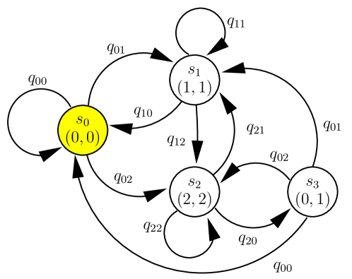
Figure 3: Transition graph of $Z=(N,\lambda)$ for $\Lambda=2$.

Example IV.2

For $\Lambda=2$, (7) provides the transition matrix

$$\mathcal{P}=\begin{bmatrix}p_{00}&p_{01}&p_{02}&p_{03}\\ p_{10}&p_{11}&p_{12}&p_{13}\\ p_{20}&p_{21}&p_{22}&p_{23}\\ p_{30}&p_{31}&p_{32}&p_{33}\end{bmatrix}=\begin{bmatrix}q_{00}&q_{01}&q_{02}&0\\ q_{10}&q_{11}&q_{12}&0\\ 0&q_{21}&q_{22}&q_{20}\\ q_{00}&q_{01}&q_{02}&0\end{bmatrix}.$$

Thus, for all $j\geq 2$, the result in (9) amounts to:

$$\mathbf{Pr}\{\Delta_{i}=j\}=\begin{bmatrix}q_{01}&q_{02}&0\end{bmatrix}\begin{bmatrix}q_{11}&q_{12}&0\\ q_{21}&q_{22}&q_{20}\\ q_{01}&q_{02}&0\end{bmatrix}^{j-2}\begin{bmatrix}q_{10}\\ 0\\ q_{00}\end{bmatrix}.$$

Particular cases of the above can be visualized by inspecting the graph in Fig. 3 as follows: The first return times $\{\Delta_{i}\}$ correspond to cycles in which $s_{0}=(0,0)$ is the starting and ending vertex, but not otherwise contained along the path. Thus, for $\Delta_{i}=2$, we have a unique cycle. It has vertices $\{s_{0},s_{1},s_{0}\}$, which gives $\mathbf{Pr}\{\Delta_{i}=2\}=q_{01}q_{10}$. For $\Delta_{i}=3$ there are three cycles, namely $\{s_{0},s_{1},s_{1},s_{0}\}$, $\{s_{0},s_{2},s_{1},s_{0}\}$, and $\{s_{0},s_{2},s_{3},s_{0}\}$. Consequently, we have $\mathbf{Pr}\{\Delta_{i}=3\}=q_{01}q_{11}q_{10}+q_{02}q_{21}q_{10}+q_{02}q_{20}q_{00}$. $\square$

V Stability Analysis

Since the processor availability is stochastic, the controller is random, see (3) and (4). In particular, if $N(k)=0$ then the plant evolves in open-loop at time $k$ (possibly using tentative plant inputs calculated at previous time-steps); if $\lambda(k)=0$, then the plant input is set to zero at that time.

Various stability notions for stochastic systems have been studied in the literature; see, e.g., [7, 8]. We focus on the following:

Definition 1

A dynamical system with state trajectory $\{x\}_{\mathbb{N}_{0}}$ is stochastically stable, if for some $\varphi\in\mathscr{K}_{\infty}$, the expected value $\sum_{k={0}}^{\infty}\mathbf{E}\big{\{}\varphi(|x(k)|)\big{\}}<\infty.$ $\square$

Assumption 3 stated below, bounds the rate of increase of $V$ in (2), when (1) is run with zero input. It also imposes a (mild) restriction on the distribution of the initial plant state.

Assumption 3

There exists $\alpha\in\mathbb{R}_{\geq 0}$ such that

$$V({f}(x,\mathbf{0}_{p}))\leq\alpha V(x),\quad\forall x\in\mathbb{R}^{n},$$ (10)

and $\mathbf{E}\big{\{}\varphi_{2}(|x(0)|)\big{\}}<\infty$, where $\varphi_{2}\in\mathscr{K}_{\infty}$ is as in (2). $\square$

It is worth noting that, since we allow for $\alpha>1$, Assumption 3 does not require that the open-loop system $x(k+1)={f}(x(k),\mathbf{0}_{p})$ be globally asymptotically stable. Further discussion on potential conservatism imposed by these assumptions can be found in Section IV-A of [15].

V-A Stability with Algorithm A₁

To study stochastic stability when Algorithm $\textsc{A}_{1}$ is used, we will focus on the random instances where the buffer runs out of control inputs.

Lemma V.1

With Algorithm A₁, the plant state sequence at the time steps $k_{i}\in\mathcal{K}$, namely $\{x\}_{\mathcal{K}}$, is Markovian. $\square$

Proof:

It follows from the definition of $k_{i}$ that $\forall k_{i}\in\mathcal{K}$ we have $u(k_{i})=\mathbf{0}_{p},$ $b(k_{i})=\mathbf{0}_{\Lambda p}$, $\lambda(k_{i})=N(k_{i})=0$. Thus, the plant state at time $k_{i+1}$ depends only on $x(k_{i})$ and $\{N(k_{i}+1),N(k_{i}+2),\dots,N(k_{i+1}-1)\}$. The result follows from the Markovian property of $\{N\}_{\mathbb{N}_{0}}$. ∎

Based on the results of Section IV and Lemma V.1, stochastic stability of the control system can be analyzed by using a stochastic Lyapunov function approach as follows:

Lemma V.2

Suppose that Assumptions 1 to 3 hold and consider $k_{0},k_{1}\in\mathcal{K}$. We then have

$$\mathbf{E}\big{\{}V(x({k_{1}}))\,\big{|}\,x(k_{0})=\chi\big{\}}\\ \leq\Omega V(\chi),\quad\forall\chi\in\mathbb{R}^{n},$$ (11)

where

$$\Omega\triangleq\alpha\sum_{j\in\mathbb{N}}\mathbf{Pr}\{\Delta_{i}=j\}\rho^{j-1}.$$ (12)

Proof:

By Lemma V.1 and Assumptions 1 and 3, we have

$$\begin{split}V(x(k_{0}+1))&\leq\alpha V(x(k_{0})),\\ V(x(k+1))&\leq\rho V(x(k)),\quad\forall k\not\in\mathcal{K}.\end{split}$$ (13)

Thus, $\mathbf{E}\big{\{}V(x({k_{1}}))\,\big{|}\,x(k_{0})=\chi,\Delta_{0}=j\big{\}}\leq\alpha\rho^{j-1}V(\chi)$, for all $\chi\in\mathbb{R}^{n}$. The result (11) follows by using the law of total expectation and the fact that $\{\Delta_{i}\}$ is i.i.d. ∎

Although Lemma V.2 considers only the instants $k_{0}$ and $k_{1}$, the bound in (11) can be used to conclude about stochastic stability for all $k\in\mathbb{N}_{0}$

Theorem V.3

Suppose that Assumptions 1–3 hold and that $\Omega<1$. Then the plant state trajectory when controlled with Algorithm A₁ is stochastically stable with the bound:

$$\sum_{k={0}}^{\infty}\mathbf{E}\big{\{}\varphi_{1}(|x(k)|)\big{\}}<\frac{1+\alpha-\rho}{(1-\Omega)(1-\rho)}\mathbf{E}\big{\{}\varphi_{2}(|x(0)|)\big{\}}.$$

Proof:

From (2) and Lemmas V.1 and V.2, it follows that if $\Omega<1$, then $V(x({k_{i}}))$ is a stochastic Lyapunov function for $\{x\}_{\mathcal{K}}$. Therefore, [8, Chapter 8.4.2, Theorem 2] implies exponential stability at instants $k_{i}\in\mathcal{K}$, i.e., for all $(i,\chi_{0})\in\mathbb{N}_{0}\times\mathbb{R}^{n}$,

$$\mathbf{E}\{V(x({k_{i}}))\,|\,x(k_{0})=\chi_{0}\}\leq\Omega^{i}V(\chi_{0}).$$

For the time steps $k\in\mathbb{N}\,\backslash\,\mathcal{K}$, i.e., where calculated control values are applied, (13) gives

$$\begin{split}\mathbf{E}&\Bigg{\{}\sum_{k=k_{i}}^{k_{i+1}-1}V(x({k}))\,\bigg{|}\,x(k_{i})=\chi_{i},\Delta_{i}=j\geq 2\Bigg{\}}\leq\Bigg{(}1+\alpha\sum_{l=0}^{j-2}\rho^{l}\Bigg{)}V(\chi_{i})\leq\bigg{(}1+\frac{\alpha}{1-\rho}\bigg{)}V(\chi_{i}).\end{split}$$

The latter bound holds for all $j\geq 2$. Now, using the law of total expectation, we obtain

$$\mathbf{E}\Bigg{\{}\sum_{k=k_{i}}^{k_{i+1}-1}V(x({k}))\,\bigg{|}\,x(k_{i})=\chi_{i}\Bigg{\}}\leq\frac{1+\alpha-\rho}{1-\rho}V(\chi_{i}).$$

Taking conditional expectation $\mathbf{E}\{\,\cdot\,|\,x(k_{0})=\chi_{0}\}$ on both sides, defining $\beta\triangleq(1+\alpha-\rho)/(1-\rho)$ and using the Markovian property of $\{x\}_{\mathcal{K}}$ yields

$$\begin{split}&\mathbf{E}\Bigg{\{}\mathbf{E}\Bigg{\{}\sum_{k=k_{i}}^{k_{i+1}-1}V(x({k}))\,\bigg{|}\,x(k_{i})=\chi_{i}\Bigg{\}}\,\Bigg{|}\,x(k_{0})=\chi_{0}\Bigg{\}}\\ &=\mathbf{E}\Bigg{\{}\sum_{k=k_{i}}^{k_{i+1}-1}V(x({k}))\,\bigg{|}\,x(k_{0})=\chi_{0}\Bigg{\}}\leq\beta\mathbf{E}\big{\{}V(x({k_{i}}))\,\big{|}\,x(k_{0})=\chi_{0}\big{\}}\leq\beta\Omega^{i}V(\chi_{0}).\end{split}$$

Thus,

$$\mathbf{E}\Bigg{\{}\sum_{k={k_{0}}}^{k_{j+1}-1}V(x({k}))\,\bigg{|}x(k_{0})=\chi_{0}\Bigg{\}}\leq\beta\sum_{i=0}^{j}\Omega^{i}V(\chi_{0}).$$

Now let $k_{j+1}\to\infty$ and recall that $k_{0}=0$ to obtain

$$\sum_{k=0}^{\infty}\mathbf{E}\big{\{}V(x(k))\,\big{|}\,x(0)=\chi_{0}\big{\}}\leq\frac{\beta}{1-\Omega}V(\chi_{0}).$$

The result now follows by using (2), Assumption 3 and taking expectation with respect to the distribution of $x(0)$. ∎

Theorem V.3 establishes sufficient conditions for stochastic stability of the control loop when Algorithm A₁ is used and processor availability is Markovian. The quantity $\Omega$ involves the contraction factor of the baseline controller $\kappa$, see (2), the bound on the rate of increase of $V$ when the plant input is zero, see (10), and the distribution of $\{\Delta_{i}\}$, $i\in\mathbb{N}_{0}$ which was characterised in Lemma IV.2. In Section VI, we will relate Theorem V.3 to the relevant result in [15]. Before doing so, we will first investigate the baseline algorithm.

V-B Stability with the Baseline Algorithm

Sufficient conditions for stochastic stability when the baseline algorithm in (3) is used can be established by proceeding in a similar manner as was done for Algorithm A₁. Here, we note that the baseline controller is characterised via:

$$u(k)=\begin{cases}\kappa(x(k))&\text{if $N(k)\in\mathbb{N}_{1}^{\Lambda}$,}\\ \mathbf{0}_{p}&\text{if $N(k)=0$}.\end{cases}$$ (14)

Denote the time steps where $N(k)=0$ as $\mathcal{T}=\{t_{i}\}$ where

$$t_{i+1}=\inf\big{\{}k\in\mathbb{N}\colon k>t_{i},\quad N(k)=0\big{\}},i\in\mathbb{N}_{0},$$

with $t_{0}=0$. Further, we introduce the process $\{\tau_{i}\}_{i\in\mathbb{N}_{0}}$ consisting of the times between consecutive elements of $\mathcal{T}$ via the relation

$$\tau_{i}=t_{i+1}-t_{i}\in\mathbb{N},\quad(t_{i},t_{i+1})\in\mathcal{T}\times\mathcal{T}.$$

Thus, $\{\tau_{i}\}_{i\in\mathbb{N}_{0}}$ are the first return times to state $0$ of the Markov Chain $\{N\}_{\mathbb{N}_{0}}$, and are therefore i.i.d. Fig. 2 can be used to visualize $\{\tau_{i}\}_{i\in\mathbb{N}_{0}}$ for the case $\Lambda=2$. This should be contrasted with how $\{\Delta_{i}\}_{i\in\mathbb{N}_{0}}$ is illustrated in Fig. 3.

By adapting the proof of Lemma IV.2, we can characterize the distribution of $\{\tau_{i}\}_{i\in\mathbb{N}_{0}}$ as follows:

Lemma V.4

Suppose that Assumption 2 holds. Then, $\mathbf{Pr}\{\tau_{i}=1\}=q_{00}$ and, for $j\geq 2$,

$$\mathbf{Pr}\{\tau_{i}=j\}=\begin{bmatrix}q_{01}&\dots&q_{0\Lambda}\end{bmatrix}\begin{bmatrix}q_{11}&\dots&q_{1\Lambda}\\ \vdots&\ddots&\vdots\\ q_{\Lambda 1}&\dots&q_{\Lambda\Lambda}\end{bmatrix}^{j-2}\begin{bmatrix}q_{10}\\ \vdots\\ q_{\Lambda 0}\end{bmatrix}\!.$$

Theorem V.5

Suppose that Assumptions 1–3 hold and that the baseline algorithm in (14) is used. If

$$\Theta\triangleq\alpha\sum_{j\in\mathbb{N}}\mathbf{Pr}\{\tau_{i}=j\}\rho^{j-1}<1,$$ (15)

then the control loop is stochastically stable. In particular,

$$\sum_{k={0}}^{\infty}\mathbf{E}\big{\{}\varphi_{1}(|x(k)|)\big{\}}<\frac{1+\alpha-\rho}{(1-\Theta)(1-\rho)}\mathbf{E}\big{\{}\varphi_{2}(|x(0)|)\big{\}}.$$

Proof:

By adapting the above ideas, it can be shown that $V(x(t_{i}))$ is a stochastic Lyapunov function for the Markov process $\{x\}_{\mathcal{T}}$. The remainder of the proof then parallels that of Theorem V.3, but using $\{\tau_{i}\}_{i\in\mathbb{N}_{0}}$ instead of $\{\Delta_{i}\}_{i\in\mathbb{N}_{0}}$. ∎

Example V.1

With $\Lambda=2$, Lemma V.4 gives that

$$\mathbf{Pr}\{\tau_{i}=j\}=\begin{cases}q_{00}&\text{if $j=1$,}\\ q_{01}q_{11}^{j-2}q_{10}&\text{if $j\geq 2$.}\end{cases}$$

in which case the sufficient condition (15) reduces to

$$\begin{split}\Theta&=\alpha q_{00}+(1-q_{00})(1-q_{11})\alpha\rho\sum_{j\geq 2}q_{11}^{j-2}\rho^{j-2}=\alpha q_{00}+\alpha\rho\frac{(1-q_{00})(1-q_{11})}{1-\rho q_{11}}\\ &=\frac{\alpha q_{00}(1-\rho q_{11})+\alpha\rho(1-q_{00})(1-q_{11})}{1-\rho q_{11}}=\frac{\alpha q_{00}(1-\rho q_{11})+\alpha\rho(1-q_{00})(1-q_{11})}{1-\rho q_{11}}<1.\end{split}$$

VI Relationship to Previous Stability Results

In Section VII of[15] we examined Algorithm A₁ using a model for the processor availability that allows for correlations in $\{N\}_{\mathbb{N}_{0}}$, by introducing a processor state process $\{g\}_{\mathbb{N}_{0}}$ with values in $\mathbb{N}_{1}^{G}$, $G\in\mathbb{N}.$ The process is described by an irreducible aperiodic Markov Chain with transition matrix $Q^{\prime}=\left[q^{\prime}_{ij}\right]_{G\times G}$ with

$$q^{\prime}_{ij}=\mathbf{Pr}\{g(k+1)=j\,|\,g(k)=i\}.$$

The realizations of $\{g\}_{\mathbb{N}_{0}}$ determine $\{N\}_{\mathbb{N}_{0}}$ as per

$$\begin{split}\mathbf{Pr}&\{N(k)=l\,|\,g(k)=\varsigma\}=p^{\prime}_{l|\varsigma},\quad\forall(l,\varsigma)\in\mathbb{N}_{0}^{\Lambda}\times\mathbb{N}_{1}^{G},\end{split}$$ (16)

with given probabilities $p^{\prime}_{l|\varsigma}$. Clearly, our model in Assumption 2 can be described using this structure by setting the processor state to satisfy $g(k)=N(k)+1,\forall k\in\mathbb{N}_{0},$ in which case $G=\Lambda+1$, and $p^{\prime}_{l|\varsigma}=1$ if $\varsigma=l+1$ and is 0 otherwise. In particular, we have $p^{\prime}_{0|\varsigma}\in\{0,1\}$ with $p^{\prime}_{0|\varsigma}=1$ if and only if $\varsigma=1$. Note that $Q^{\prime}=\mathcal{Q}$ since

$$q^{\prime}_{ij}=\mathbf{Pr}\{g(k+1)=j\,|\,g(k)=i\}=\mathbf{Pr}\{N(k+1)+1=j\,|\,N(k)+1=i\}=q_{i-1,j-1}.$$

VI-A The Baseline Algorithm

Given the above, for the model in Assumption 2, Theorem 4 of [15] establishes that if $\alpha<1$, then the closed loop system when using the baseline algorithm is stochastically stable. This is in contrast to the results in our current work, which also allow for $\alpha>1$. Thus, Theorem V.5 provides a sufficient condition which can also be used for open-loop unstable plant models. This follows directly from Lemma V.4 and by the fact that $\rho\in[0,1)$, so that

$$\sum_{j\in\mathbb{N}}\mathbf{Pr}\{\tau_{i}=j\}\rho^{j-1}=q_{00}+\sum_{j=2}^{\infty}\mathbf{Pr}\{\tau_{i}=j\}\rho^{j-1}\leq q_{00}+\rho\sum_{j\geq 2}\mathbf{Pr}\{\tau_{i}=j\}=q_{00}+\rho(1-q_{00})<1.$$

VI-B The Anytime Algorithm

Application of Theorem 5 of[15] to our present model gives the following sufficient condition for stochastic stability, that is proven in Appendix C.

Corollary VI.1

Let Assumptions 1–3 hold. Suppose that $\alpha q_{00}<1$ and that $\Upsilon_{\varsigma}<1,\forall\varsigma\in\mathbb{N}_{2}^{\Lambda+1},$ where

$$\Upsilon_{\varsigma}\triangleq\frac{q_{(\varsigma-1)0}(1-q_{00})}{1-q_{00}\rho}\Bigg{(}\frac{(\alpha-\rho)}{1-q_{00}\alpha}q_{00}^{\varsigma-2}\rho^{\varsigma-1}+\rho^{2}\Bigg{)}+\rho(1-q_{(\varsigma-1)0}).$$ (17)

Then the plant state trajectory when controlled with Algorithm A₁ is stochastically stable. $\square$

In general, comparing the above sufficient condition with the one presented in Theorem V.3 is difficult. To elucidate the situation, in the remainder of this section we will focus on processor availability models where all transition probabilities are equal, i.e.,

$$q_{ij}=1/(\Lambda+1),\quad\forall i,j\in\mathbb{N}_{0}^{\Lambda}.$$ (18)

For this class of models, the result in (9) can be written as:

$$\mathbf{Pr}\{\Delta_{i}=j\}=(1/(\Lambda+1))^{j}\sum_{k=1}^{\Lambda}\sum_{l=1}^{\Lambda}v_{kl}\lambda_{k}^{j-2},\quad j\geq 2,$$ (19)

where $\{\lambda_{k}\}$, $k\in\mathbb{N}_{1}^{\Lambda}$, are the non-zero eigenvalues of $\underline{\mathcal{P}}\triangleq(1/(\Lambda+1))^{2-j}\overline{P}$, $\{v_{k}\}$ are the corresponding eigenvectors such that $\mu^{T}v_{k}\neq 0$, and $v_{kl}$ denotes the $l$-th element of $v_{k}$. Expressions (12) and (19) yield

$$\begin{split}\Omega&=(\alpha/(\Lambda+1))+\alpha\rho\sum_{j\geq 2}(1/(\Lambda+1))^{j}\sum_{k=1}^{\Lambda}\sum_{l=1}^{\Lambda}v_{kl}(\lambda_{k}\rho)^{j-2}=(\alpha/(\Lambda+1))\bar{f}_{\Lambda}(\rho),\end{split}$$

where

$$\bar{f}_{\Lambda}(\rho)\triangleq 1+\frac{\rho}{\Lambda+1}\Bigg{(}\sum_{k=1}^{\Lambda}\frac{1}{1-\lambda_{k}\rho/(\Lambda+1)}\sum_{l=1}^{\Lambda}v_{kl}\Bigg{)}=1+\rho\sum_{k=1}^{\Lambda}\frac{\lambda_{k}v_{k1}}{\Lambda+1-\lambda_{k}\rho}.$$

Therefore, $\alpha\leq({\Lambda+1})/{\bar{f}_{\Lambda}(\rho)}\Leftrightarrow\Omega\leq 1$.

On the other hand, with $q_{00}\alpha<1$, (17) yields

$$\begin{split}\Upsilon_{2}&=\frac{\rho q_{10}(1-q_{00})}{1-q_{00}\rho}\Bigg{(}\frac{(\alpha-\rho)}{1-q_{00}\alpha}+\rho\Bigg{)}+\rho(1-q_{10})=\rho+\frac{\rho(\alpha-1)q_{10}}{1-q_{00}\alpha}=\frac{\rho\Lambda}{\Lambda+1-\alpha},\quad\forall\Lambda\geq 2.\end{split}$$

Thus $\alpha\leq\Lambda+1-\Lambda\rho\Leftrightarrow\Upsilon_{2}\leq 1$. Recalling that $\alpha q_{00}<1$, $q_{ij}=1/(\Lambda+1),~{}\forall i,j\in\mathbb{N}_{0}^{\Lambda}$ and $\rho<1$, it follows that $\Upsilon_{2}\geq\Upsilon_{\varsigma}$, for all $\varsigma\in\mathbb{N}_{2}^{\Lambda+1}$.

The above analysis leads to the following characterization on cases where the stability condition developed in this work is less conservative than the one presented in [15].

Corollary VI.2

Consider a processor availability model of the form (18) and suppose that $\alpha<\Lambda+1$. If

$${\bar{f}_{\Lambda}(\rho)}(\Lambda+1-\Lambda\rho)<\Lambda+1,$$

then the sufficient condition for stability in Theorem 5 of[15] is more conservative than the one derived in Theorem V.3 of the present work. $\square$

Additional comparisons are provided in Section VIII.

Example VI.1

For $\Lambda=2$, the result in (9) amounts to:

$$\mathbf{Pr}\{\Delta_{i}=j\}=(1/3)^{j}\begin{bmatrix}1&1&0\end{bmatrix}\begin{bmatrix}1&1&0\\ 1&1&1\\ 1&1&0\end{bmatrix}^{j-2}\begin{bmatrix}1\\ 0\\ 1\end{bmatrix},\quad j\geq 2.$$ (20)

By decomposing $[1\;0\;1]^{T}$ into the eigenvectors of the matrix above, we obtain

$$\begin{split}&\begin{bmatrix}1&1&0\end{bmatrix}\begin{bmatrix}1&1&0\\ 1&1&1\\ 1&1&0\end{bmatrix}^{j-2}\begin{bmatrix}1\\ 0\\ 1\end{bmatrix}=\begin{bmatrix}1&1&0\end{bmatrix}\begin{bmatrix}1&1&0\\ 1&1&1\\ 1&1&0\end{bmatrix}^{j-2}\left(\begin{bmatrix}1/2\\ \sqrt{2}/2\\ 1/2\end{bmatrix}+\begin{bmatrix}1/2\\ -\sqrt{2}/2\\ 1/2\end{bmatrix}\right)\\ &=\begin{bmatrix}1&1&0\end{bmatrix}(1+\sqrt{2})^{j-2}\begin{bmatrix}1/2\\ \sqrt{2}/2\\ 1/2\end{bmatrix}+\begin{bmatrix}1&1&0\end{bmatrix}(1-\sqrt{2})^{j-2}\begin{bmatrix}1/2\\ -\sqrt{2}/2\\ 1/2\end{bmatrix},\end{split}$$

so that

$$\mathbf{Pr}\{\Delta_{i}=j\}=(1/3)^{j}\frac{(1+\sqrt{2})^{j-1}+(1-\sqrt{2})^{j-1}}{2},\quad j\geq 2.$$ (21)

Thus (and after some algebraic manipulations), (12) yields

$$\begin{split}\Omega&=(\alpha/3)+\frac{\alpha}{2}\sum_{j\geq 2}(1/3)^{j}(1+\sqrt{2})^{j-1}\rho^{j-1}+\frac{\alpha}{2}\sum_{j\geq 2}(1/3)^{j}(1-\sqrt{2})^{j-1}\rho^{j-1}=(\alpha/3)\bar{f}_{2}(\rho).\end{split}$$ (22)

where

$$\bar{f}_{2}(\rho)\triangleq 1+(\rho/2)\Bigg{(}\frac{(1+\sqrt{2})(3-\rho(1-\sqrt{2}))+(1-\sqrt{2})(3-\rho(1+\sqrt{2}))}{(3-\rho(1+\sqrt{2}))(3-\rho(1-\sqrt{2}))}\Bigg{)}=\frac{3(3-\rho)}{9-6\rho-\rho^{2}}.$$ (23)

Using Corollary VI.2 and by noting that

$$(3-2\rho)\bar{f}_{2}(\rho)\leq 3\Longleftrightarrow\rho(1-\rho)\geq 0,$$ (24)

we conclude that the upper bound on $\alpha$ permited in Theorem 5 of [15] is smaller than the one allowed in the present work. $\square$

VII Robustness To Process Noise

Our presentation so far assumed no process noise in (1). A natural question is if the quality of future inputs, and hence the performance of the algorithm, degrades if process noise is present. We now consider the case where the system model is given by

$$x(k+1)=f(x(k),u(k),w(k)),$$ (25)

where $w(k)\in\mathbb{R}^{n}$ is a white noise process, assumed independent of the other random variables in the system. For simplicity we shall assume uniform continuity and bounds as follows:

Assumption 4

There exist $\lambda_{x},\lambda_{u},\lambda_{w},\lambda_{V},\lambda_{\kappa},\rho,\beta,\alpha,\eta\in\mathbb{R}_{\geq 0}$ such that, $\forall x,z,w\in\mathbb{R}^{n}$ and $\forall u,v\in\mathbb{R}^{p}$ the following are satisfied:

$$\begin{split}|f(x,u,w)-f(z,v,\mathbf{0}_{n})|&\leq\lambda_{x}|x-z|+\lambda_{u}|u-v|+\lambda_{w}|w|,\\ |V(x)-V(z)|&\leq\lambda_{V}|x-z|,\\ |\kappa(x)-\kappa(z)|&\leq\lambda_{\kappa}|x-z|,\end{split}$$ (26)

$$\begin{split}V(f(x,\kappa(x),w))&\leq\rho V(x)+\beta|w|,\\ V(f(x,\mathbf{0}_{p},w))&\leq\alpha V(x)+\eta|w|.\end{split}$$ (27)

The following result shows that the condition $\Omega<1$, used in Theorem V.3, plays an important role also in the present robustness analysis. As in related results on stochastic stability with unbounded dropouts and disturbances (see, e.g., [16]), the property established is weaker than that of Theorem V.3.

Theorem VII.1

Suppose that Assumptions 1–4 hold, that $\mathbf{E}\{|w(k)|\}<\infty$ and that $\Omega<1$. Then the plant state trajectory when controlled with Algorithm A₁ satisfies $\mathbf{E}\{\varphi_{1}(|x(k)|)\}<\infty$, $\forall k\in\mathbb{N}_{0}.$ $\square$

VIII Case Studies

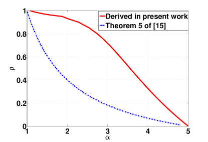
Figure 4: Boundaries of stability regions for the example considered.

We consider a processor availability model with $\Lambda=5$ and the transition probability matrix $\mathcal{Q}$ with $q_{00}=0.2,~{}q_{0j}=0.16,~{}\forall j\in\mathbb{N}_{1}^{\Lambda},~{}q_{10}=0.9,~{}q_{11}=q_{12}=0.05,~{}q_{21}=0.1,~{}q_{2j}=0.225,~{}\forall j\in\mathbb{N}_{2}^{\Lambda},~{}q_{ij}=0.25,~{}\forall i\in\mathbb{N}_{3}^{\Lambda},~{}\forall j\in\mathbb{N}_{2}^{\Lambda}$. All other transition probabilities are identically zero:

$$\mathcal{Q}=\begin{bmatrix}0.2&0.16&0.16&0.16&0.16&0.16\\ 0.9&0.05&0.05&0&0&0\\ 0&0.1&0.225&0.225&0.225&0.225\\ 0&0&0.25&0.25&0.25&0.25\\ 0&0&0.25&0.25&0.25&0.25\\ 0&0&0.25&0.25&0.25&0.25\end{bmatrix}.$$

Intuitively, since the sufficient condition for stability in Corollary VI.1 is based on a worst case analysis, whereas the condition in Theorem V.3 is not, the latter result can be expected to be less conservative than the former. This conjecture was verified in Example VI.1 and is further illustrated in Fig. 4 that characterizes the stability region boundaries in terms of $\alpha$ and $\rho$. The stable region (area under the curve) as derived from the condition given in Theorem V.3 is larger than the one derived from Corollary VI.1 (which embodies Theorem 5 of [15]).

Figure 5: Empirical cost when controlling (28) with the anytime algorithm and with the baseline algorithm (14), as a function of the parameter $\Lambda$, see (29). Also included is the ideal case with unlimited resources, where $u(k)=\kappa(x(k))$, for all $k\in\mathbb{N}$.

Next, consider a specific non-linear plant model of the form (1), where

$$x(k+1)=x(k)+0.01((x(k))^{3}+u(k)).$$ (28)

A control law satisfying Assumption 1 is given by $\kappa(x)=-x^{3}-x$, which is globally stabilizing with $V(x)=|x|$, $\varphi_{1}(|x|)=\varphi_{2}(|x|)=|x|$ and $\rho=0.99$, see [15]. Consider the following class of processor availability transition matrices:

$$\mathcal{Q}_{\Lambda}=\begin{bmatrix}0.4&0.6/\Lambda&0.6/\Lambda&\dots\\ 0.6/\Lambda&0.4&0.6/\Lambda&\dots\\ 0.6/\Lambda&0.6/\Lambda&0.4&\ddots\\ \vdots&\vdots&\ddots&\ddots\end{bmatrix}\in\mathbb{R}^{(\Lambda+1)\times(\Lambda+1)}.$$ (29)

In (29), $\Lambda\in\{1,2,\dots,7\}$ is a parameter which determines the support of $\{N\}_{\mathbb{N}_{0}}$ and also how likely the processor availability changes. We adopt as performance measure, the empirical cost

$$J=\frac{1}{50}\mathbf{E}\left\{\sum_{k=0}^{49}\left(0.2(x(k))^{2}+2(u(k))^{2}\right)\right\},$$

where expectation is taken with respect to the process $\{N\}_{\mathbb{N}_{0}}$. Fig. 5 illustrates the result obtained when using the anytime algorithm A₁ and also the baseline algorithm (14). The anytime control algorithm outperforms the baseline controller for all processor availability models considered. Fig. 5 also compares the performance with the one without computational uncertainty, i.e. $N(k)>0,~{}\forall k$. This comparison characterizes the degradation in performance due to fluctuating CPU time.

IX Conclusions

We analyzed an anytime control algorithm when the processor availability is described by a Markov Chain. The algorithm partially compensates for the effect of the processor not providing sufficient resources at some time steps. For general non-linear systems, we used stochastic Lyapunov methods to obtain sufficient conditions for stability. The results obtained complement those of our recent article [15]. In subsequent work, see[13], we have shown how to use the present analysis methodology for networked control systems with random delays and dropouts.

Appendix A Proof of Lemma IV.1

If Assumption 2 holds, the definition of $\mathbb{S}$, (5) and the Markovian property of $\{N\}_{\mathbb{N}_{0}}$ yield:

$$\begin{split}p_{00}&=\mathbf{Pr}\{Z(k+1)=s_{0}\,|\,Z(k)=s_{0}\}=\mathbf{Pr}\{N(k+1)=\lambda(k+1)=0\,|\,N(k)=\lambda(k)=0\}\\ &=\mathbf{Pr}\{N(k+1)=0\,|\,N(k)=0\}=q_{00}\\ p_{10}&=\mathbf{Pr}\{Z(k+1)=s_{0}\,|\,Z(k)=s_{1}\}=\mathbf{Pr}\{N(k+1)=\lambda(k+1)=0\,|\,N(k)=\lambda(k)=1\}\\ &=\mathbf{Pr}\{N(k+1)=0\,|\,N(k)=1\}=q_{10}\\ p_{(\Lambda+1)0}&=\mathbf{Pr}\{Z(k+1)=s_{0}\,|\,Z(k)=s_{\Lambda+1}\}=\mathbf{Pr}\{N(k+1)=\lambda(k+1)=0\,|\,N(k)=0,\lambda(k)=1\}\\ &=\mathbf{Pr}\{N(k+1)=0\,|\,N(k)=0\}=q_{00}.\end{split}$$

Similarly, for all $(i,j)\in\mathbb{N}_{0}^{\Lambda}\times\mathbb{N}_{1}^{\Lambda}$, one has

$$p_{ij}=\mathbf{Pr}\{Z(k+1)=s_{j}\,|\,Z(k)=s_{i}\}=\mathbf{Pr}\{N(k+1)=j\,|\,N(k)=i\}=q_{ij},$$

whereas, for all $j\in\mathbb{N}_{1}^{\Lambda-1}$, the transition probabilities satisfy

$$\begin{split}p_{(j+1)(\Lambda+j)}&=\mathbf{Pr}\{Z(k+1)=s_{\Lambda+j}\,|\,Z(k)=s_{j+1}\}=\mathbf{Pr}\{Z(k+1)=(0,j)\,|\,Z(k)=(j+1,j+1)\}\\ &=\mathbf{Pr}\{N(k+1)=0\,|\,N(k)=j+1\}=q_{(j+1)0}.\end{split}$$

Direct calculations also yield that for all $m\in\mathbb{N}_{2}^{\Lambda-1}$,

$$\begin{split}p&{}_{(\Lambda+m)(\Lambda+m-1)}=\mathbf{Pr}\{Z(k+1)=s_{\Lambda+m-1}\,|\,Z(k)=s_{\Lambda+m}\}\\ &=\mathbf{Pr}\{Z(k+1)=(0,m-1)\,|\,Z(k)=(0,m)\}=\mathbf{Pr}\{N(k+1)=0\,|\,N(k)=0\}=q_{00},\end{split}$$

and, for all $(k,l)\in\mathbb{N}_{1}^{\Lambda-1}\times\mathbb{N}_{1}^{\Lambda}$, it holds that $p_{(\Lambda+k)l}=\mathbf{Pr}\{Z(k+1)=s_{l}\,|\,Z(k)=s_{\Lambda+k}\}=\mathbf{Pr}\{Z(k+1)=(l,l)\,|\,Z(k)=(0,k)\}=\mathbf{Pr}\{N(k+1)=l\,|\,N(k)=0\}=q_{0l}.$ Due to (5), the other transitions will never occur.

Appendix B Proof of Lemma IV.2

The case $j=1$ is immediate, since $\mathbf{Pr}\{\Delta_{i}=1\}=\mathbf{Pr}\{Z(k+1)=(0,0)\,|\,Z(k)=(0,0)\}=\mathbf{Pr}\{N(k+1)=0\,|\,N(k)=0\}=q_{00}$. For $j\geq 2$, we proceed as follows: For all $s_{i}\in\mathbb{S}$, $i\not=0$, denote by $\nu_{i}$ the first passage time of the state $s_{i}$ to $s_{0}$. Thus, $\nu_{i}$ are random variables, with $\nu_{i}=j$ if the state $s_{0}$ is entered from $s_{i}$ for the first time in $j$ steps. Since only the states $s_{1}$ and $s_{\Lambda+1}$ can reach $s_{0}$ in one step, using (8),

$$\mathbf{Pr}\{\nu_{i}=1\}=p_{i0}=\begin{cases}q_{10},&\text{if $i=1$}\\ q_{00},&\text{if $i=\Lambda+1$}\\ 0,&\text{if $i\in\mathbb{N}_{2}^{\Lambda}\cup\mathbb{N}_{\Lambda+2}^{2\Lambda-1}$.}\end{cases}$$ (30)

For $j\geq 2$, paths from $s_{i}$ to $s_{0}$ go through intermediate states $s_{\ell}\not=s_{0}$, providing the recursions

$$\mathbf{Pr}\{\nu_{i}=j\}=\sum_{\ell=1}^{2\Lambda-1}p_{i\ell}\mathbf{Pr}\{\nu_{\ell}=j-1\},\quad\forall i\in\mathbb{N}_{1}^{2\Lambda-1},$$

which can be stated in matrix form via:

$$\begin{bmatrix}\mathbf{Pr}\{\nu_{1}=j\}\\ \vdots\\ \mathbf{Pr}\{\nu_{2\Lambda-1}=j\}\end{bmatrix}=\overline{\mathcal{P}}\begin{bmatrix}\mathbf{Pr}\{\nu_{1}=j-1\}\\ \vdots\\ \mathbf{Pr}\{\nu_{2\Lambda-1}=j-1\}\end{bmatrix}=\overline{\mathcal{P}}^{j-1}\begin{bmatrix}\mathbf{Pr}\{\nu_{1}=1\}\\ \vdots\\ \mathbf{Pr}\{\nu_{2\Lambda-1}=1\}\end{bmatrix}=\overline{\mathcal{P}}^{j-1}\mu,$$

which in view of (30) and (8), holds not only for $j\geq 2$ , but also for $j=1$. The result now follows by using (30) and the distribution of $\{\Delta_{i}\}$. The latter can be obtained from the distribution of $\nu_{i}$ by considering the transitions from $s_{0}$ to nodes other than itself (see (8)):

$$\mathbf{Pr}\{\Delta_{i}=j\}=\sum_{\ell=1}^{2\Lambda-1}p_{0\ell}\mathbf{Pr}\{\nu_{\ell}=j-1\}=\sum_{\ell=1}^{\Lambda}q_{0\ell}\mathbf{Pr}\{\nu_{\ell}=j-1\}.$$

Appendix C Proof of Corollary VI.1

For the situation of interest, the term $\Upsilon_{\varsigma}$ introduced in Lemma 4 of[15] can be written as:

$$\begin{split}\Upsilon_{\varsigma}&=\bar{q}_{\varsigma}\big{(}I-\rho\bar{Q}\big{)}^{-1}\,\bigg{(}\rho I+(\alpha-\rho)\big{(}I-\alpha\bar{Q}\big{)}^{-1}\sum_{l=1}^{\Lambda}p_{l|\varsigma}(\rho\bar{Q})^{l}\bigg{)}\bar{p}\\ \end{split}$$ (31)

for all $\varsigma\in\{2,3,\dots,\Lambda+1\}$ and where

$$\begin{split}\bar{q}_{\varsigma}&=\begin{bmatrix}q_{(\varsigma-1)0}&q_{(\varsigma-1)1}&\dots&q_{(\varsigma-1)\Lambda}\end{bmatrix},\quad\bar{Q}=\begin{bmatrix}q_{00}&q_{01}&\dots&q_{0\Lambda}\\ 0&0&\dots&0\\ \vdots&\vdots&\ddots&\vdots\\ 0&0&\dots&0\end{bmatrix}\!,\;\bar{p}=\begin{bmatrix}0\\ 1\\ \vdots\\ 1\end{bmatrix}\end{split}$$

Direct calculations lead to $\bar{Q}^{l}=(q_{00})^{l-1}\bar{Q}$, for all $l\in\mathbb{N}$ and (31) is then condensed into

$$\begin{split}\Upsilon_{\varsigma}&=\bar{q}_{\varsigma}\big{(}I-\rho\bar{Q}\big{)}^{-1}\Big{(}\rho I+\rho^{\varsigma-1}(q_{00})^{\varsigma-2}(\alpha-\rho)\big{(}I-\alpha\bar{Q}\big{)}^{-1}\bar{Q}\Big{)}\bar{p}\\ &=\frac{1}{1-q_{00}\rho}\Bigg{(}\frac{(\alpha-\rho)}{1-q_{00}\alpha}q_{00}^{\varsigma-2}\rho^{\varsigma-1}+\rho^{2}\Bigg{)}\sum_{l=1}^{\Lambda}q_{(\varsigma-1)0}q_{0l}+\rho\sum_{l=1}^{\Lambda}q_{(\varsigma-1)l},\end{split}$$

which proves the result.

Appendix D Proof of Theorem VII.1

To establish this result, we first extend Lemma V.2 to the perturbed plant case (25). Clearly, for $\Delta_{0}\geq 1$ (and setting $k_{0}=0$, $x(0)=x$, and using notation $\mathbf{E}_{x}\{\cdot\}=\mathbf{E}\{\cdot\,|\,x(0)=x\}$), we have $u(0)=\mathbf{0}_{p}$. Thus,

$$V(x(1))\leq\alpha V(x)+\eta|w(0)|,\quad\forall\Delta_{0}\geq 1$$

so that

$$\mathbf{E}_{x}\{V(x(1))\,|\,\Delta_{0}\geq 1\}\leq\alpha V(x)+W\Psi_{1}(0),$$

where $W\triangleq\mathbf{E}\{|w(k)|\}$ and $\Psi_{1}(0)=\eta$. Now for $\Delta_{0}\geq 2$, thus $u(1)=\kappa((x(1))$, using the above we obtain

$$V(x(2))\leq\rho V(x(1))+\beta|w(1)|\leq\rho\alpha V(x(0))+\rho\eta|w(0)|+\beta|w(1)|,\quad\forall\Delta_{0}\geq 2$$ (32)

yielding

$$\mathbf{E}_{x}\{V(x(2))\,|\,\Delta_{0}\geq 2\}\leq\alpha\rho V(x)+W\Psi_{2}(1),$$

with $\Psi_{2}(1)=\rho\eta+\beta$.

For $\Delta_{0}\geq 3$ analyzing $V(x(3))$ becomes more involved since $u(2)$ could have been calculated using $x(1)$ or $x(2)$:

$$u(2)\in\{\kappa(x(2)),\kappa(\bar{f}(x(1)))\}$$ (33)

where

$$\bar{f}(x)\triangleq f(x,\kappa(x),\mathbf{0}_{n}).$$ (34)

For notational convenience, we let $\bar{f}^{0}(x)\triangleq x$ and define the result of two repeated iterations of (34) as $\bar{f}^{2}(x)\triangleq f(\bar{f}(x),\kappa(\bar{f}(x)),\mathbf{0}_{n})$, and $\bar{f}^{k}(x)$ as the result of $k$ repeated iterations of (34). Interestingly, due to continuity, both cases in (33) are not that far away from $\kappa(x(2))$. In fact,

$$\begin{split}|u(2)-\kappa(x(2))|&\leq|\kappa(\bar{f}(x(1)))-\kappa(x(2))|\leq\lambda_{\kappa}|\bar{f}(x(1))-x(2)|\\ &=\lambda_{\kappa}|f(x(1),\kappa(x(1)),\mathbf{0}_{n})-f(x(1),\kappa(x(1)),w(1))|\leq\lambda_{\kappa}\lambda_{w}|w(1)|.\end{split}$$

Thus,

$$\begin{split}&|f(x(2),u(2),w(2))-f(x(2),\kappa(x(2)),w(2))|\\ &\leq|f(x(2),\kappa(\bar{f}(x(1))),w(2))-f(x(2),\kappa(x(2)),w(2))|\leq\lambda_{u}\lambda_{\kappa}\lambda_{w}|w(1)|\end{split}$$

which using (32) gives

$$\begin{split}V(x(3))&=V(f(x(2),\kappa(x(2)),w(2)))+V(x(3))-V(f(x(2),\kappa(x(2)),w(2)))\\ &\leq\rho V(x(2))+\beta|w(2)|+\lambda_{V}\lambda_{u}\lambda_{\kappa}\lambda_{w}|w(1)|\\ &\leq\alpha\rho^{2}V(x(0))+\rho^{2}\eta|w(0)|+\rho\beta|w(1)|+\beta|w(2)|+\lambda_{V}\lambda_{u}\lambda_{\kappa}\lambda_{w}|w(1)|,\quad\forall\Delta_{0}\geq 3\end{split}$$ (35)

and

$$\mathbf{E}_{x}\{V(x(3))\,|\,\Delta_{0}\geq 3\}\leq\alpha\rho^{2}V(x)+W\Psi_{3}(2)$$

with

$$\Psi_{3}(j)=\sum_{\ell=0}^{j}\psi_{3,\ell}\rho^{\ell},\quad\psi_{3,0}=\beta+\lambda_{V}\lambda_{u}\lambda_{\kappa}\lambda_{w},\;\psi_{3,1}=\beta,\;\psi_{3,2}=\eta,$$

To extend the above analyis to $V(x(4))$ for $\Delta_{0}\geq 4$, simply note that (for $\Lambda\geq 3$),

$$u(3)\in\big{\{}\kappa(x(3)),\kappa(\bar{f}(x(2))),\kappa\big{(}\bar{f}(\bar{f}(x(1)))\big{)}\big{\}},$$

thus,

$$|u(3)-\kappa(x(3))|\leq\max\big{\{}|\kappa(\bar{f}(x(2)))-\kappa(x(3))|,|\kappa(\bar{f}^{2}(x(1)))-\kappa(x(3))|\big{\}}$$

By examining both cases separately, an upper bound can be obtained. For example, for $u(3)=\kappa(\bar{f}^{2}(x(1)))$, we have

$$\begin{split}|\kappa(\bar{f}^{2}(x(1)))-\kappa(x(3))|&\leq\lambda_{\kappa}|\bar{f}^{2}(x(1))-x(3)|\\ &\leq\lambda_{\kappa}|f(\bar{f}(x(1)),\kappa(\bar{f}(x(1)),\mathbf{0}_{n})-f(x(2),\kappa(x(2)),w(2))|\\ &\leq\lambda_{\kappa}\bigg{[}(\lambda_{x}+\lambda_{u}\lambda_{\kappa})|\bar{f}(x(1)-x(2)|+\lambda_{w}|w(2)|\bigg{]}\\ &\leq\lambda_{\kappa}(\lambda_{x}+\lambda_{u}\lambda_{\kappa})\lambda_{w}|w(1)|+\lambda_{\kappa}\lambda_{w}|w(2)|.\end{split}$$

leading to

$$\begin{split}&|f(x(3),u(3),w(3))-f(x(3),\kappa(x(3)),w(3))|\\ &\leq|f(x(3),\kappa(\bar{f}^{2}(x(1))),w(3))-f(x(3),\kappa(x(3)),w(3))|\\ &\leq\lambda_{u}\bigg{[}\lambda_{\kappa}(\lambda_{x}+\lambda_{u}\lambda_{\kappa})\lambda_{w}|w(1)|+\lambda_{\kappa}\lambda_{w}|w(2)|\bigg{]}\end{split}$$

which gives (using (35))

$$\begin{split}V(x(4))&=V(f(x(3),\kappa(x(3)),w(3)))+V(x(4))-V(f(x(3),\kappa(x(3)),w(3)))\\ &\leq\rho V(x(3))+\beta|w(3)|+\lambda_{V}\lambda_{u}\bigg{[}\lambda_{\kappa}(\lambda_{x}+\lambda_{u}\lambda_{\kappa})\lambda_{w}|w(1)|+\lambda_{\kappa}\lambda_{w}|w(2)|\bigg{]}\\ &\leq\alpha\rho^{3}V(x(0))+\rho^{3}\eta|w(0)|+\bigg{(}\rho^{2}\beta+\rho\lambda_{V}\lambda_{u}\lambda_{\kappa}\lambda_{w}+\lambda_{V}\lambda_{u}\lambda_{\kappa}(\lambda_{x}+\lambda_{u}\lambda_{\kappa})\lambda_{w}\bigg{)}|w(1)|\\ &+(\rho\beta+\lambda_{V}\lambda_{u}\lambda_{\kappa}\lambda_{w})|w(2)|+\beta|w(3)|,\quad\forall\Delta_{0}\geq 4.\end{split}$$

For the case $u(3)=\kappa(\bar{f}(x(2)))$, a similar expression can be obtained, leading to a common upper-bound of the form:

$$\mathbf{E}_{x}\{V(x(4))\,|\,\Delta_{0}\geq 4\}\leq\alpha\rho^{3}V(x(0))+W\Psi_{4}(3),$$

where $\Psi_{4}(j)=\sum_{\ell=0}^{j}\psi_{4,\ell}\rho^{\ell}$, $j\leq 3$.

To continue the analysis presented above, for $\Delta_{0}\geq j,~{}j\geq 5$ (for $\Lambda\geq j-1$), we note that

$$u(j-1)\in\big{\{}\kappa(x(j-1)),\kappa(\bar{f}(x(j-2))),...,\kappa\big{(}\bar{f}^{l-1}(x(j-l))\big{)},~{}l=1,...,j-1\big{\}},$$

Following similar ideas, one obtains

$$\mathbf{E}_{x}\{V(x(j))\,|\,\Delta_{0}\geq j\}\leq\alpha\rho^{j-1}V(x(0))+W\Psi_{j}(j-1),$$ (36)

where $\Psi_{j}(j-1)=\sum_{\ell=0}^{j-1}\psi_{j,\ell}\rho^{\ell}$. Notice that, since the buffer length $\Lambda$ is bounded, the terms $\psi_{j,\ell},~{}\forall j\in\mathbb{N},~{}\ell\in\mathbb{N}_{0}^{j-1}$ are bounded.

The above analysis allows one to generalize Lemma V.2 to the case with i.i.d. disturbances. The law of total expectation, the fact that $\{\Delta_{i}\}$ is i.i.d., and expression (36) give

$$\mathbf{E}\big{\{}V(x({k_{1}}))\,\big{|}\,x(k_{0})=\chi\big{\}}\\ \leq\Omega V(\chi)+\Sigma,\quad\forall\chi\in\mathbb{R}^{n},$$ (37)

where

$$\Sigma\triangleq\sum_{j\in\mathbb{N}}\mathbf{Pr}\{\Delta_{i}=j\}W\Psi_{j}(j-1).$$

From (2) and (37) and since Lemma V.1 holds also in the perturbed case, it follows that if $\Omega<1$, then for all $(i,\chi_{0})\in\mathbb{N}_{0}\times\mathbb{R}^{n}$,

$$\mathbf{E}\{V(x({k_{i}}))\,|\,x(k_{0})=\chi_{0}\}\leq\Omega^{i}V(\chi_{0})+\big{(}\Omega^{i-1}+\Omega^{i-2}+...+\Omega+1\big{)}\Sigma.$$

For the time steps $k\in\mathbb{N}\,\backslash\,\mathcal{K}$, i.e., where calculated control values are applied, (36) and the law of total expectation yield

$$\mathbf{E}\Bigg{\{}\sum_{k=k_{i}}^{k_{i+1}-1}V(x({k}))\,\bigg{|}\,x(k_{i})=\chi_{i}\Bigg{\}}\leq\bigg{(}1+\frac{\alpha}{1-\rho}\bigg{)}V(\chi_{i})+W^{\prime},$$

where

$$W^{\prime}\triangleq\sum_{j\geq 2}\mathbf{Pr}\{\Delta_{i}=j\}W\Psi_{j}(j-2)<\infty,$$

with $\Psi_{j}(j-2)=\sum_{\ell=0}^{j-2}\psi_{j,\ell}\rho^{\ell}$. Taking conditional expectation $\mathbf{E}\{\,\cdot\,|\,x(k_{0})=\chi_{0}\}$ on both sides, defining $\beta\triangleq(1+\alpha-\rho)/(1-\rho)$ and using the Markovian property of $\{x\}_{\mathcal{K}}$ yields

$$\begin{split}&\mathbf{E}\Bigg{\{}\mathbf{E}\Bigg{\{}\sum_{k=k_{i}}^{k_{i+1}-1}V(x({k}))\,\bigg{|}\,x(k_{i})=\chi_{i}\Bigg{\}}\,\Bigg{|}\,x(k_{0})=\chi_{0}\Bigg{\}}=\mathbf{E}\Bigg{\{}\sum_{k=k_{i}}^{k_{i+1}-1}V(x({k}))\,\bigg{|}\,x(k_{0})=\chi_{0}\Bigg{\}}\\ &\leq\beta\mathbf{E}\big{\{}V(x({k_{i}}))\,\big{|}\,x(k_{0})=\chi_{0}\big{\}}+W^{\prime}\\ &\leq\beta\Omega^{i}V(\chi_{0})+\beta\bigg{(}\Omega^{i-1}+\Omega^{i-2}+...+\Omega+1\bigg{)}\Sigma+W^{\prime}\end{split}$$

Thus,

$$\mathbf{E}\Big{\{}V(x({k}))\,\big{|}\,x(k_{0})=\chi_{0}\Big{\}}\leq\beta\Omega V(\chi_{0})+\beta\bigg{(}\sum_{\ell=0}^{i-1}\Omega^{\ell}\bigg{)}\Sigma+W^{\prime},\quad\forall k\in\{k_{i},k_{i}+1\dots,k_{i+1}-1\}.$$

Now recall that $k_{0}=0$ and that

$$\bigcup_{i\in\mathbb{N}_{0}}\{k_{i},k_{i}+1\dots,k_{i+1}-1\}=\mathbb{N}_{0}.$$

The result now follows by using (2), Assumption 3 and taking expectation with respect to the distribution of $x(0)$.

References

• [1] R. Bhattacharya and G. J. Balas, “Anytime Control Algorithms: Model Reduction Approach,” AIAA Journal of Guidance, Control and Dynamics, 27(5), September-October 2004.
• [2] A. Cervin, M. Velasco, P. Marti, and A. Camacho, “Optimal On-Line Sampling Period Assignment: Theory and Experiments,” IEEE Transactions on Control Systems Technology, 18(5):1-9, June, 2010.
• [3] L. Greco, D. Fontanelli, and A. Bicchi, “Design and stability analysis for anytime control via stochastic scheduling,” IEEE Trans. Automat. Contr., vol. 56, pp. 571–585, Mar. 2011.
• [4] V. Gupta, “On a Control Algorithm for Time-varying Processor Availability,” Hybrid Systems, Control and Computation Conference (HSCC), April 2010.
• [5] D. Henriksson and J. Akesson, “Flexible Implementation of Model Predictive Control using Sub-optimal Solutions,” Internal Report No. TFRT-7610-SE, Dep. of Automatic Control, Lund University, 2004.
• [6] D. Henriksson, A. Cervin, J. Akesson and K. E. Arzen, “On Dynamic Real-Time Scheduling of Model Predictive Controllers,” In Proc. IEEE Conf. Decis. Contr., (Las Vegas, NV), Dec. 2002.
• [7] Y. Ji, H. J. Chizeck, X. Feng, and K. A. Loparo, “Stability and control of discrete-time jump linear systems,” Control Theory Advanced Technology, 7(2): 247-270, 1991.
• [8] H. J. Kushner, “Introduction to Stochastic Control,” Holt, Rinehart and Winston Inc., New York N.Y.
• [9] J. G. Kemeny and J. L. Snell, Finite Markov Chains. D. Van Nostrand Company, Inc, 1960.
• [10] L. K. McGovern and E. Feron, “Requirements and Hard Computational Bounds for Real-time Optimization in Safety Critical Control Systems,” IEEE Conference on Decision and Control (CDC 98), 1998.
• [11] L. K. McGovern and E. Feron, “Closed-loop Stability of Systems Driven by Real-Time Dynamic Optimization Algorithms,” IEEE Conference on Decision and Control (CDC 99), 1999.
• [12] J. Nilsson, B. Bernhardsson and B. Wittenmark, “Stochastic analysis and control of real-time systems with random time delays,” Automatica, vol. 34, no. 1, pp. 57–64, 1998.
• [13] D. E. Quevedo and I. Jurado, “Stability of sequence-based control with random delays and dropouts,” IEEE Trans. Automat. Contr., in press, DOI: 10.1109/TAC.2013.2286911.
• [14] D. E. Quevedo and V. Gupta, “Stability of sequence-based anytime control with Markovian processor availability,” in Proc. Austr. Contr. Conf., 2011.
• [15] D. E. Quevedo and V. Gupta, “Sequence-based anytime control,” IEEE Trans. Automat. Contr., 58(2), 377-390, February. 2013.
• [16] D. E. Quevedo and D. Nešić, “Robust stability of packetized predictive control of nonlinear systems with disturbances and Markovian packet losses,” Automatica, vol. 48, pp. 1803–1811, Aug. 2012.
• [17] P. Tabuada, “Event-triggered real-time scheduling of stabilizing control tasks,” IEEE Transactions on Automatic Control, 52(9), 1680-1685, September 2007.
• [18] M. Velasco, P. Marti, and E. Bini, “On Lyapunov Sampling for Event-driven Controllers,” IEEE CDC 2009.
• [19] X. Wang and M. D. Lemmon, “Self-triggered Feedback Control Systems with Finite-Gain L2 Stability,” IEEE Transactions on Automatic Control, 45(3):452-,2009.