A multi-band semiclassical model for surface hopping quantum dynamics

Abstract

In the paper we derive a semiclassical model for surface hopping allowing quantum dynamical non-adiabatic transition between different potential energy surfaces in which cases the classical Born-Oppenheimer approximation breaks down. The model is derived using the Wigner transform and Weyl quantization, and the central idea is to evolve the entire Wigner matrix rather than just the diagonal entries as was done previously in the adiabatic case. The off-diagonal entries of the Wigner matrix suitably describe the non-adiabatic transition, such as the Berry connection, for avoided crossings. We study the numerical approximation issues of the model, and then conduct numerical experiments to validate the model.

1 Introduction

In this paper we derive a semiclassical model based on the quantum phase-space description of the particle dynamics. We consider the nucleonic Schrödinger system:

$$\mathrm{i}\varepsilon\frac{\partial\psi^{\varepsilon}}{\partial t}(t,\boldsymbol{x}) =\hat{H}\psi^{\varepsilon}(t,x),\qquad\left(t,\boldsymbol{x}\right)\in\left(\mathbb{R}^{+},\mathbb{R}^{d}\right)$$ (1.1)

$$\psi^{\varepsilon}(0,\boldsymbol{x}) =\psi^{\varepsilon}_{0}(\boldsymbol{x})$$ (1.2)

with the self-adjoint Hamiltonian operator defined by:

$$\hat{H}=-\frac{\varepsilon^{2}}{2}\Delta_{\boldsymbol{x}}+\tilde{V}(\boldsymbol{x}).$$ (1.3)

Here, $\psi$ is a vector and $\tilde{V}(x)$ is a Hermitian matrix. $\varepsilon=\sqrt{\frac{m}{M}}$ is the mass ratio between electron and nuclei. This system arises from the Born-Oppenheimer approximation [5] of the $N-$body Schrödinger equation in which the nucleonic Schrödinger system (1.1) is solved along the electronic potential surfaces. We will focus on the two-energy system although our study can be extended to systems with more energy levels in a straightforward way. In the two-energy level case, the potential matrix reads as:

$$\begin{split}\tilde{V}(\boldsymbol{x})&=\frac{1}{2}\text{tr}\tilde{V}(\boldsymbol{x})+V=U(\boldsymbol{x})+\left(\begin{array}[]{cc}u(\boldsymbol{x})&v(\boldsymbol{x})\\ v^{\dagger}(\boldsymbol{x})&-u(\boldsymbol{x})\end{array}\right).\end{split}$$ (1.4)

For future references, we consider the unitary matrix $\Theta$

$$\Theta^{\dagger}(\boldsymbol{x})=\left[\chi_{+},\chi_{-}\right],$$ (1.5)

that diagonalizes the potential operator $V$. We have

$$V=\Theta^{\dagger}\Lambda_{V}\Theta,$$ (1.6)

where

$$\Lambda_{V}(\boldsymbol{x})=\mathrm{diag}\big{(}E(\boldsymbol{x}),\,-E(\boldsymbol{x})\big{)}=\mathrm{diag}\left(\sqrt{|u(\boldsymbol{x})|^{2}+|v(\boldsymbol{x})|^{2}},-\sqrt{|u(\boldsymbol{x})|^{2}+|v(\boldsymbol{x})|^{2}}\right),$$ (1.7)

and

$$\begin{split}\Theta&=\frac{1}{\sqrt{2\,\left(1+\frac{u(\boldsymbol{x})}{E(\boldsymbol{x})}\right)}}\left(\begin{array}[]{rr}\left(1+\frac{u(\boldsymbol{x})}{E(\boldsymbol{x})}\right)\frac{v^{\dagger}(\boldsymbol{x})}{|v(\boldsymbol{x})|}&\frac{|v(\boldsymbol{x})|}{E(\boldsymbol{x})}\\ -\frac{v^{\dagger}(\boldsymbol{x})}{E(\boldsymbol{x})}&1+\frac{u(\boldsymbol{x})}{E(\boldsymbol{x})}\end{array}\right).\end{split}$$ (1.8)

Obviously $\chi_{\pm}$ are the eigenvectors of $V$ corresponding to the eigenvalues $\pm E$ with $E(\boldsymbol{x})=\sqrt{|u(\boldsymbol{x})|^{2}+|v(\boldsymbol{x})|^{2}}$. Hereafter, we call the two eigenvalues the energy bands, and $\Delta{E}=2E$, the energy gap.

For $\Delta E=0$, the matrix $\Theta$ becomes singular (conical crossing). In this paper, we are interested in the cases where the energy gap is strictly positive and asymptotically small. In particular, we focus on the so called avoided crossing scaling where the minimum of the energy gap is of the order $\sqrt{\varepsilon}$.

We consider a few types of prototype potentials and analyze their influence on the non-adiabatic transitions process:

1D case:

$$u(x)=x,\quad v(x,\delta)\equiv\delta,\quad U(\boldsymbol{x})=0.$$ (1.9)

The eigenvalues are $\Lambda_{V}^{\pm}=\pm E=\pm\sqrt{x^{2}+\delta^{2}}$ and the avoided crossing point is $x=0$.

2D cases:

First example

$$u(\boldsymbol{x},\delta)=x,\quad v(\boldsymbol{x},\delta)=\sqrt{y^{2}+\delta^{2}},\quad U(\boldsymbol{x})=0.$$ (1.10)

Second example

$$u(\boldsymbol{x},\delta)=x,\quad v(\boldsymbol{x},\delta)=y+\mathrm{i}\delta,\quad U(\boldsymbol{x})=0.$$ (1.11)

Here, we denoted $\boldsymbol{x}=(x,y)$. In the 2D cases, the eigenvalues are given by $\Lambda_{V}^{\pm}=\pm E=\pm\sqrt{x^{2}+y^{2}+\delta^{2}}$, and the avoided crossing point is $(x,y)=(0,0)$.

We are interested in deriving a semiclassical approximation to the Schrödinger system (1.1) with avoided-crossings. One of the advantages of our method is that the computational cost is significantly reduced than solving directly the original Schrödinger system (1.1).

One of the difficulties in the derivation of the semiclassical expansion for a system with two or more energy levels, is the non-commutativity of the matrix $\tilde{V}$ with the Laplacian operator. In the case where $\Delta{E}$ is of order 1, the equation of motion can be well approximated by a fully diagonalized system – one classical Liouville equation for each energy level [30, 27, 13, 14, 15, 20, 1, 39, 41, 38]. This is the standard Born-Oppenheimer approximation. See reviews [12, 42]. However, when the eigenvalues are of $O(\sqrt{\varepsilon})$ away from each other, the classical Born-Oppenheimer approximation breaks down and the diagonalized system is no longer a good approximation of the full coupled system. In such case, around the crossing points, the particles could move from one band to another (the non-adiabatic phenomenon).

The study of the mathematical properties and the study of the physical systems where the energy band structure shows some crossing points dates back to Wigner and von Neumann [45]. It can be shown that the crossing set is of measure zero, while the influence is of order $1$, and it is this crossing phenomenon that is responsible of some chemical reactions [47, 49]. Due to its physical significance, this topic has been studied extensively in computational chemistry community. The first result on the transition rate is due to Landau and Zener [50], who gave a rough estimate on the transition probability. Afterwards, there is very rich literature investigating the different aspects of the problem, including theoretical studies and algorithm development. We here mention the two most well-known algorithms, both by Tully etc.: the surface hopping method based on applying Landau-Zener formula [43], and the fewest switches method [44], a Markov-Chain Monte-Carlo type method. Some criticisms have been also raised on the Landau-Zener formula, and we mention [3, 21].

On the mathematical side, in [16] Hagedorn firstly rigorously reexamined Zener’s idea. This was followed by a series of works [28, 27, 23, 19, 18, 40, 6], in which they also show that the jumping behavior could heavily depends on the types of crossings (see classification of crossings in [17]). The study of the non-adiabatic transition on the phase space was done in [8].

The surface hopping algorithms that use the Landau-Zener formula for evaluating the non-adiabatic transitions for conical crossings have seen recent mathematical interests [31, 25, 24, 9]. The main advantage of these surface hopping methods, compared to computing the original Schrödinger equation (1.1), is that they do not need to numerically resolve the $O(\varepsilon)$ wavelength. However, these methods cannot account for phase information at the crossing points, and thus ignore important physical phenomenon [4, 37]. The main result of this paper is to present a semiclassical model that includes the particle phase correction at the crossing points.

Our method is based on the Wigner transform [33] and the Weyl quantization [46, 22] procedure. In the adiabatic case, with $\varepsilon\to 0$ (classical limit), the Wigner transformation leads to a set of decoupled Liouville equations, each for one energy band [33, 10]. In this case, only the diagonal entries of the Wigner matrix that correspond to the projection onto the two eigenspaces of the underlying Hamiltonian are relevant. However, in the presence of a band crossing, one cannot ignore the off-diagonal terms. For this reason, our main idea in the paper is to find the semiclassical approximation for the entire Wigner matrix. This approach is similar to the derivation of the transport equation for graphene [35] and in semiconductors systems [36]. Our model is a coupled Liouville system for all entries of the Wigner matrix, where the off-diagonal terms prescribes the quantum transition between bands, and the two-bands correlations due to the Berry connections. We also discuss numerical approximation of this model utilizing a multi-physics domain decomposition idea proposed in [7]: away from the crossing points we solve the standard adiabatic Liouville equations, while in the crossing zones the new semiclassical system is solved, and the two systems are connected by interface conditions.

In section 2 we present the derivation of the new semiclassical model. We also produce a primitive analysis of the behavior of the solutions to the system. In section 3 we describe a coupling method that combines the new semiclassical model near the crossing points with the adiabatic system elsewhere in order to further reduce the computational cost. Numerical examples are shown afterwards.

2 The semiclassical formulation

In the following we describe the basics of the Wigner transform and the Weyl quantization. In subsections 2.2 and 2.3 we derive the mathematical model for the adiabatic and non-adiabatic cases respectively.

2.1 The Wigner transformation and Weyl quantization

The Wigner function is defined by

$$F^{\varepsilon}(\boldsymbol{x},\boldsymbol{p})=\frac{1}{(2\pi)^{d}}\int\,\rho^{\varepsilon}\left(\boldsymbol{x}-\frac{\varepsilon\boldsymbol{y}}{2},\boldsymbol{x}+\frac{\varepsilon\boldsymbol{y}}{2}\right)\,\mathrm{e}^{{\mathrm{i}}\boldsymbol{p}\cdot\boldsymbol{y}}\,\mathrm{d}\boldsymbol{y},$$ (2.1)

where $\rho^{\varepsilon}(\boldsymbol{x},\boldsymbol{x}^{\prime})=\psi^{\varepsilon}(\boldsymbol{x})\otimes\overline{\psi^{\varepsilon}}(\boldsymbol{x}^{\prime})$ is the density matrix, $\psi^{\varepsilon}$ is defined in (1.1), $\overline{\psi^{\varepsilon}}$ is the complex conjugate of $\psi^{\varepsilon}$. The Wigner function is defined in a quadratic manner, so it is insensitive to a constant phase shift.

The moments of the Wigner distribution function taken with respect to the momentum variable, provide the physical observables of the system. In particular, the position density and flux are given by

$$\rho^{\varepsilon}(\boldsymbol{x},t) =|\psi^{\varepsilon}|^{2}=\int_{\mathbb{R}^{d}}F^{\varepsilon}\mathrm{d}\boldsymbol{p},\quad J^{\varepsilon}(\boldsymbol{x},t) =\varepsilon\text{Im}\left(\bar{\psi}^{\varepsilon}\cdot\nabla_{\boldsymbol{x}}\psi^{\varepsilon}\right)=\int_{\mathbb{R}^{d}}\boldsymbol{p}F^{\varepsilon}\mathrm{d}\boldsymbol{p}.$$ (2.2)

The evolution of the Wigner function is governed by the Wigner equation

$$\partial_{t}{F^{\varepsilon}}+\boldsymbol{p}\cdot\nabla_{\boldsymbol{x}}{F^{\varepsilon}}+\Xi[U\mathbb{I}+V]F^{\varepsilon}=0,$$ (2.3)

where $\Xi[V]$ is defined as

$$\begin{split}\Xi[V]F^{\varepsilon}&=\frac{1}{(2\pi)^{d}}\int_{\mathbb{R}^{2d}}\,\frac{\mathrm{i}}{\varepsilon}\,\left[{V\left(\boldsymbol{x}-\frac{\varepsilon\boldsymbol{y}}{2}\right)F^{\varepsilon}(\boldsymbol{x},\boldsymbol{p}^{\prime})-F^{\varepsilon}(\boldsymbol{x},\boldsymbol{p}^{\prime})V\left(\boldsymbol{x}+\frac{\varepsilon\boldsymbol{y}}{2}\right)}\right]\mathrm{e}^{\mathrm{i}(\boldsymbol{p}^{\prime}-\boldsymbol{p})\cdot\boldsymbol{y}}\mathrm{d}\boldsymbol{p}^{\prime}\,\mathrm{d}\boldsymbol{y}.\end{split}$$

We note that $F$ and $V$ are matrices, and in general they do not commute.

A quantum mechanical operator can be univocally associated to a function $A(\boldsymbol{x},\boldsymbol{p})$ defined on the classical phase-space by the so called Weyl quantization [46, 34]. The following map is used

$$\mathcal{W}(A)[h](\boldsymbol{x})=\hat{A}[h](\boldsymbol{x})={\frac{1}{(2\pi\varepsilon)^{d}}}\int\int\,A\left(\frac{\boldsymbol{x}+\boldsymbol{y}}{2},\boldsymbol{p}\right)\,h(\boldsymbol{x},\boldsymbol{y})\,\mathrm{e}^{\frac{\mathrm{i}}{\varepsilon}(\boldsymbol{x}-\boldsymbol{y})\cdot\boldsymbol{p}}\,\mathrm{d}\boldsymbol{p}\,\mathrm{d}\boldsymbol{y}.$$ (2.4)

Here, $\hat{A}\equiv\mathcal{W}(A)$ is the Weyl quantum mechanical operator defined on the space of the smooth functions $h(\boldsymbol{x},\boldsymbol{y})\in\mathcal{S}(\mathbb{R}^{d}\times\mathbb{R}^{d})$. The function $A(\boldsymbol{x},\boldsymbol{p})$ denotes the symbol of $\hat{A}$. It is easy to verify that the Weyl quantization map is the inverse of the Wigner transform (the Weyl quantization procedure applied to the Wigner function $F^{\varepsilon}$ provides the density operator).

In particular, the Weyl quantization of the Hamiltonian is the Schrödinger operator. Namely,

$$A(\boldsymbol{x},\boldsymbol{p})=H(\boldsymbol{x},\boldsymbol{p})=\frac{\boldsymbol{p}^{2}}{2}+\tilde{V}(\boldsymbol{x})\quad\Rightarrow\quad\hat{A}=\hat{H}=-\frac{\varepsilon^{2}}{2}\Delta_{\boldsymbol{x}}+\tilde{V}(\boldsymbol{x}).$$ (2.5)

The use of the Wigner-Moyal formalism is eased by the definition of the Moyal product $\#$ as

$$A\#B:= \frac{1}{(2\pi)^{2d}}\int{}A\left(\boldsymbol{x}-\frac{\varepsilon}{2}\boldsymbol{\eta},\boldsymbol{p}+\frac{\varepsilon}{2}\boldsymbol{\mu}\right)B(\boldsymbol{x}^{\prime},\boldsymbol{p}^{\prime})e^{\mathrm{i}(\boldsymbol{x}-\boldsymbol{x}^{\prime})\cdot\boldsymbol{\mu}+\mathrm{i}(\boldsymbol{p}-\boldsymbol{p}^{\prime})\cdot\boldsymbol{\eta}}\mathrm{d}\boldsymbol{\mu}\mathrm{d}\boldsymbol{x}^{\prime}\mathrm{d}\boldsymbol{\eta}\mathrm{d}\boldsymbol{p}^{\prime}$$

$$= A\mathrm{e}^{\frac{\mathrm{i}\varepsilon}{2}\left(\overleftarrow{\nabla}_{\boldsymbol{x}}\cdot\overrightarrow{\nabla}_{\boldsymbol{p}}-\overleftarrow{\nabla}_{\boldsymbol{p}}\cdot\overrightarrow{\nabla}_{\boldsymbol{x}}\right)}B,$$ (2.6)

where the arrows indicate on which symbol the gradients act. An important property of the Moyal product is $\mathcal{W}(A\#B)=\mathcal{W}(A)\mathcal{W}(B)$. The #-product admits an $\varepsilon$-expansion. The $O(\varepsilon)$ term is the classical Poisson bracket $\{A,B\}=\nabla_{\boldsymbol{p}}A\cdot\nabla_{\boldsymbol{x}}B-\nabla_{\boldsymbol{x}}A\cdot\nabla_{\boldsymbol{p}}B$, and

$$A\#B=AB-\frac{\mathrm{i}\varepsilon}{2}\{A,B\}+{O}(\varepsilon^{2}).$$ (2.7)

2.2 The adiabatic case

The mathematical study of the semiclassical limit in the adaibatic case was carried out in [33, 10]. According to Theorem 6.1 in [10], outside the crossing set $S=\{\boldsymbol{x}:\,\lambda^{+}(\boldsymbol{x})=\lambda^{-}(\boldsymbol{x})\}$, the Wigner function can be obtained by the projection of the solution onto the eigenspaces of the Hamiltonian. Let $F^{0}(t,\boldsymbol{x},\boldsymbol{p})\doteq\lim_{\varepsilon\rightarrow 0}F(t,\boldsymbol{x},\boldsymbol{p})$, we have

$$F^{0}(t,\cdot) =\Pi_{+}F^{0}(t,\cdot)\Pi_{+}+\Pi_{-}F^{0}(t,\cdot)\Pi_{-}$$ (2.8a)

$$=f^{+}(t,\cdot)\Pi_{+}+f^{-}(t,\cdot)\Pi_{-},$$ (2.8b)

where

$$\Pi_{\pm}(\boldsymbol{x})=\chi^{\pm}(\boldsymbol{x})\otimes\chi^{\pm}(\boldsymbol{x})$$

and $f^{\pm}$ are the particle densities related to energy levels $\lambda^{\pm}(\boldsymbol{x},\boldsymbol{k})$

$$f^{\pm}=\mathrm{Tr}(\Pi_{\pm}F^{0}(t,\cdot)).$$ (2.9)

The distributions $f^{\pm}$ satisfy the classical Liouville equation:

$$\partial_{t}f^{\pm}+\nabla_{\boldsymbol{p}}\lambda^{\pm}\cdot\nabla_{\boldsymbol{x}}f^{\pm}-\nabla_{\boldsymbol{x}}\lambda^{\pm}\cdot\nabla_{\boldsymbol{p}}f^{\pm}=0,\quad t>0,\;\boldsymbol{x}\in\mathbb{R}^{d}\setminus{S},\;\boldsymbol{p}\in\mathbb{R}^{d},$$ (2.10a)

$$f^{\pm}(t=0,\boldsymbol{x},\boldsymbol{p})=\mathrm{Tr}(\Pi_{\pm}F^{0}(t=0,\boldsymbol{x},\boldsymbol{p})).$$ (2.10b)

2.3 Quantum transition in the non-adiabatic case

In the proximity of the crossing points, the Born-Oppenheimer approximation is no longer valid. By using the Wigner formalism, we derive a semiclassical model that is able to treat the quantum mechanical band transitions in the case where the separation between the upper and lower energy levels scales as $\sqrt{\varepsilon}$. In particular, the transitions between bands are captured by the off-diagonal terms of the Wigner matrix distribution. Our approach is alternative to the use of the Landau-Zener formula for the evaluation of the transition probability in correspondence to an avoided crossing and overcomes some of the difficulties that affect the Landau-Zener approach as argued in [21]. We follow the derivation presented in [35, 29].

Starting from the von Neumann equation, we have:

$$\mathrm{i}\varepsilon\frac{\partial\hat{F}^{\prime}}{\partial t} =\left[\hat{H}^{\prime},\hat{F}^{\prime}\right].$$ (2.11)

where we have defined

$$\hat{F}^{\prime}=\hat{\Theta}\,\hat{\rho}\,\hat{\Theta}^{\dagger},\quad\hat{H}^{\prime}=\hat{\Theta}\,\hat{H}\,\hat{\Theta}^{\dagger}.$$ (2.12)

Here, $\hat{\Theta}=\mathcal{W}[\Theta]$ and $\hat{\Theta}^{\dagger}$ are the Weyl quantization of $\Theta$ and $\Theta^{\dagger}$ respectively. In particular, $\hat{\Theta}\hat{V}\hat{\Theta}^{\dagger}=\hat{\Lambda}_{V}$.

Equation (2.11) is a diagonalized version of the von Neumann equation written on the Weyl operator formalism. To obtain an equivalent dynamical system defined on the quantum phase-space, we usd the inverse Weyl mapping:

$$\mathrm{i}\varepsilon\frac{\partial{F}^{\prime}}{\partial t}=\left[{H}^{\prime},{F}^{\prime}\right]_{\#},$$ (2.13)

where $\left[A,B\right]_{\#}=A\#B-B\#A$ is a commutator of the Moyal product (2.1), and $H^{\prime}$ and $F^{\prime}$ are symbols associated with $\hat{H^{\prime}}$ and $\hat{F^{\prime}}$ respectively:

$$H^{\prime}(\boldsymbol{x},\boldsymbol{p})=\Theta(\boldsymbol{x})\#H(\boldsymbol{x},\boldsymbol{p})\#\Theta(\boldsymbol{x})^{\dagger},\qquad F^{\prime}(\boldsymbol{x},\boldsymbol{p})=\Theta(\boldsymbol{x})\#F(\boldsymbol{x},\boldsymbol{p})\#\Theta(\boldsymbol{x})^{\dagger}.$$ (2.14)

By using (2.7), we expand the equation (2.13)

$$\mathrm{i}\varepsilon\frac{\partial{F}^{\prime}}{\partial t}= [\Lambda,F^{\prime}]-\frac{\mathrm{i}\varepsilon}{2}\{\Lambda,F\}+\frac{\mathrm{i}\varepsilon}{2}\{F,\Lambda\}+\mathrm{i}\varepsilon[\boldsymbol{p}\cdot\nabla_{\boldsymbol{x}}\Theta\,\Theta^{\dagger},F^{\prime}]\;+\;O(\varepsilon^{2})$$

$$\begin{split}=&[\Lambda,F^{\prime}]-\frac{\mathrm{i}\varepsilon}{2}[\nabla_{\boldsymbol{p}}\Lambda,\nabla_{\boldsymbol{x}}F]_{+}+\frac{\mathrm{i}\varepsilon}{2}[\nabla_{\boldsymbol{x}}\Lambda,\nabla_{\boldsymbol{p}}F]_{+}\\ &\quad\quad\quad+\,\mathrm{i}\varepsilon\,[\boldsymbol{p}\cdot\nabla_{\boldsymbol{x}}\Theta\,\Theta^{\dagger},F^{\prime}]\;+\;O(\varepsilon^{2}),\end{split}$$ (2.15)

with $[A,B]_{+}=AB+BA$. Keeping up to the second order in $\varepsilon$ (see Appendix for details):

$$H^{\prime}(\boldsymbol{x},\boldsymbol{p})=\Lambda(\boldsymbol{x},\boldsymbol{p})+\mathrm{i}\varepsilon\boldsymbol{p}\cdot\nabla_{\boldsymbol{x}}\Theta(\boldsymbol{x})\Theta^{\dagger}(\boldsymbol{x})+\frac{\varepsilon^{2}}{2}\nabla_{\boldsymbol{x}}\Theta(\boldsymbol{x})\cdot\nabla_{\boldsymbol{x}}\Theta^{\dagger}(\boldsymbol{x}).$$ (2.16)

By ignoring the $O(\varepsilon^{2})$ terms, the evolution equations then become (for details of the asymptotic derivation see Appendix)

$$\frac{\partial f^{+}}{\partial t} =-\boldsymbol{p}\cdot\nabla_{\boldsymbol{x}}f^{+}+\nabla_{\boldsymbol{x}}\big{(}U+E\big{)}\cdot\nabla_{\boldsymbol{p}}f^{+}+\bar{b}^{i}f^{i}+b^{i}\overline{f^{i}},$$ (2.17a)

$$\frac{\partial f^{-}}{\partial t} =-\boldsymbol{p}\cdot\nabla_{\boldsymbol{x}}f^{-}+\nabla_{\boldsymbol{x}}\big{(}U-E\big{)}\cdot\nabla_{\boldsymbol{p}}f^{-}-\bar{b}^{i}f^{i}-b^{i}\overline{f^{i}},$$ (2.17b)

$$\frac{\partial f^{i}}{\partial t} =-\boldsymbol{p}\cdot\nabla_{\boldsymbol{x}}f^{i}\,+\nabla_{\boldsymbol{x}}U\cdot\nabla_{\boldsymbol{p}}f^{i}+b^{i}(f^{-}-f^{+})+(b^{+}-b^{-})f^{i}+\frac{2E}{\mathrm{i}\varepsilon}f^{i},$$ (2.17c)

where we have denoted

$$F^{\prime} =\left(\begin{array}[]{cc}f^{+}&f^{i}\\ \bar{f}^{i}&f^{-}\end{array}\right),\quad\text{and}\quad\boldsymbol{p}\cdot\nabla_{\boldsymbol{x}}\Theta\,\Theta^{\dagger}=\left(\begin{array}[]{cc}b^{+}&b^{i}\\ -\bar{b}^{i}&b^{-}\end{array}\right).$$ (2.22)

In vector form (2.17) becomes:

$$\frac{\partial\boldsymbol{f}}{\partial t}+\boldsymbol{p}\cdot\nabla_{\boldsymbol{x}}\boldsymbol{f}-\nabla_{\boldsymbol{x}}A\cdot\nabla_{\boldsymbol{p}}\boldsymbol{f}=C\boldsymbol{f}+\frac{D}{\mathrm{i}\varepsilon}\boldsymbol{f}$$ (2.23a)

where:

$$\boldsymbol{f} =\left(f^{+},\,f^{-},\,f^{i},\,\overline{f^{i}}\right)^{T},$$ (2.23b)

$$A =\text{diag}\left(U+E,\,U-E,\,U,\,U\right),$$ (2.23c)

$$D =\text{diag}\left(0,\,0,\,2E,\,-2E\right),$$ (2.23d)

$$C =\left(\begin{array}[]{cccc}0&0&\overline{b^{i}}&b^{i}\\ 0&0&-\overline{b^{i}}&-b^{i}\\ -b^{i}&b^{i}&b^{+}-b^{-}&0\\ -\overline{b^{i}}&\overline{b^{i}}&0&b^{+}-b^{-}\end{array}\right).$$ (2.23i)

Here, $f^{\pm}$, both real, represent the projection coefficients onto the positive and negative energy bands. The function $f^{i}$ describes the transition between the two bands.

Specifically for the three examples in (1.9), (1.10) and (1.11), we have explicit formulae for $b^{s}$, $s\in\{\pm,i\}$:

For (1.9):

$b^{+}=b^{-}\equiv 0,\quad\text{and}\quad b^{i}=-\frac{p\delta}{2(x^{2}+\delta^{2})}$.

For (1.10):

denote $\boldsymbol{p}=(p,q)$, then

$$b^{+}=b^{-}\equiv 0,\quad b^{i}=\frac{1}{2(x^{2}+y^{2}+\delta^{2})}\left(\frac{qxy}{\sqrt{y^{2}+\delta^{2}}}-p\sqrt{y^{2}+\delta^{2}}\right).$$ (2.24)

For (1.11):

one has for $\boldsymbol{p}=(p,q)$, $E=\sqrt{x^{2}+y^{2}+\delta^{2}}$ and

$$\begin{split}b^{+}&=\frac{q\delta\left(E+x\right)}{2E^{3}}\mathrm{i}\;,\quad b^{-}=\frac{q\delta}{2E(E+x)}\mathrm{i}\;,\\ b^{i}&=\frac{1}{2(x^{2}+y^{2}+\delta^{2})}\left\{\left(\frac{qxy}{\sqrt{y^{2}+\delta^{2}}}-p\sqrt{y^{2}+\delta^{2}}\right)-\mathrm{i}q\delta\right\}.\end{split}$$ (2.25)

The system (2.23) is hyperbolic, $\Theta$ is unitary, $b^{\pm}$ are purely imaginary, and the matrix $C$ is skew Hermitian.

Remark 2.1.

According to the adiabatic theory [48, 35], when time $t$ is sufficiently small, the solution of the Schrödinger equation (1.1) can be written as

$$\psi^{\varepsilon}(t)=\psi_{+}(t)+\psi_{-}(t),$$

with $$\;\psi_{\pm}(t)=\mathrm{e}^{\mathrm{i}\gamma_{\pm}(t)}\exp\left(\mp\frac{\mathrm{i}}{\varepsilon}\int_{0}^{t}\mathrm{d}{t^{\prime}}E(\boldsymbol{x}(t^{\prime}))\right)\chi_{\pm}(\boldsymbol{x}(t)),$$ (2.26)

where $\boldsymbol{x}(t)$ is a semiclassical trajectory. For $t=0$, the initial state coincides with the eigenstate $\chi_{s}(\boldsymbol{x}(0))$ for $s\in\{+,-\}$. The second exponential in (2.1) is known as the dynamical phase factor, and $\gamma_{\pm}$ in the first exponential is the path integral of the Berry connection, i.e.

$$\gamma_{\pm}(t)=\mathrm{i}\int\,\dot{\boldsymbol{x}}(t)\cdot\big{(}\nabla_{\boldsymbol{x}}\chi_{\pm}(\boldsymbol{x}(t))\cdot\chi_{\pm}^{\dagger}(\boldsymbol{x}(t)\big{)}\,\mathrm{d}{t},$$ (2.27)

which is called the Berry phase. This term cancels out in the diagonal term of the density function $\psi_{+}^{\dagger}\psi_{+}$ and $\psi_{-}^{\dagger}\psi_{-}$. However for the off diagonal term $\psi_{-}^{\dagger}{\psi}_{+}$, we have

$$\begin{split}\psi_{-}^{\dagger}{\psi}_{+}(\boldsymbol{x}(t))=&\exp\left\{\mathrm{i}\left(\gamma_{+}(t)-\gamma_{-}(t)-\frac{2}{\varepsilon}\int_{0}^{t}\mathrm{d}{t^{\prime}}E(\boldsymbol{x}(t^{\prime}))\right)\right\}\chi_{-}^{\dagger}(\boldsymbol{x}(t))\chi_{+}(\boldsymbol{x}(t))\,.\end{split}$$ (2.28)

By evaluating the derivative of the Berry phase we have

$$\begin{split}&\mathrm{i}\frac{\mathrm{d}}{\mathrm{d}{t}}\left(\gamma_{+}(t)-\gamma_{-}(t)-\frac{2}{\varepsilon}\int_{0}^{t}\mathrm{d}{t^{\prime}}E(\boldsymbol{x}(t^{\prime}))\right)\\ =&-\dot{\boldsymbol{x}}(t)\cdot\big{(}\nabla_{\boldsymbol{x}}\chi_{+}\cdot\chi_{+}^{\dagger}-\nabla_{\boldsymbol{x}}\chi_{-}\cdot\chi_{-}^{\dagger}\big{)}-\frac{2\mathrm{i}}{\varepsilon}E(\boldsymbol{x}(t)).\end{split}$$ (2.29)

If we apply $\dot{\boldsymbol{x}}=\boldsymbol{p}$ where $\boldsymbol{p}$ is the momentum, then we get

$$\begin{split}&\mathrm{i}\frac{\mathrm{d}}{\mathrm{d}{t}}\left(\gamma_{+}(t)-\gamma_{-}(t)-\frac{2}{\varepsilon}\int_{0}^{t}\mathrm{d}{t^{\prime}}E(\boldsymbol{x}(t^{\prime}))\right)=\big{(}b^{+}(\boldsymbol{x}(t))-b^{-}(\boldsymbol{x}(t))\big{)}-\frac{2\mathrm{i}}{\varepsilon}E(\boldsymbol{x}(t))\,.\end{split}$$ (2.30)

Comparing with (2.17c), one can see that these are exactly the coefficients of the $f^{i}$ terms in (2.17c). This shows our model indeed captures the Berry phase in the inter-band transition processes.

3 A hybrid model by domain decomposition

The equation (2.17) is a hyperbolic system, with a transport part and a source term. Concerning the numerical treatment of Eq. (2.17) the major difficulties arise form the term $\frac{2E}{\mathrm{i}\varepsilon}$ in the equation for $f^{i}$. It introduces rapid oscillations in both space and time that demand high computational cost. In order to reduce the numerical complexity, we solve the semiclassical model (2.17) only in the proximity of the crossing zone. Away form the crossing points we neglect the band transitions and solve the adiabatic model

$$\frac{\partial f^{+}}{\partial t} = -\boldsymbol{p}\cdot\nabla_{\boldsymbol{x}}f^{+}+\nabla_{\boldsymbol{x}}\big{(}U+E\big{)}\cdot\nabla_{\boldsymbol{p}}f^{+},$$ (3.1a)

$$\frac{\partial f^{-}}{\partial t} = -\boldsymbol{p}\cdot\nabla_{\boldsymbol{x}}f^{-}+\nabla_{\boldsymbol{x}}\big{(}U-E\big{)}\cdot\nabla_{\boldsymbol{p}}f^{-}.$$ (3.1b)

A similar hybrid model was used in [7] for the Schrödinger equation with a periodic lattice potential.

As an example, consider the one-dimensional case with $p>0$ (so that in the $x$ space the wave packet moves from the left to the right). The other cases are treated similarly. We decompose the domain into the following two regions:

The adiabatic region:

$x<-C_{0}\sqrt{\varepsilon}$ and $x>C_{0}\sqrt{\varepsilon}$:
In this region, we use $o(1)$ coarse mesh, independent of $\varepsilon$ for the adiabatic Liouville system (3.1). $f^{i}$ is set to be zero. At $x=-C_{0}\sqrt{\varepsilon}$, no boundary condition is required, while at $x=C_{0}\sqrt{\varepsilon}$, we impose the inflow boundary condition that $f^{+}$ and $f^{-}$ are given by the solution inside the non-adiabatic region discussed below.

The non-adiabatic region:

$\left[-C_{0}\sqrt{\varepsilon},\quad C_{0}\sqrt{\varepsilon}\right]$:
In this region we use $o(\sqrt{\varepsilon})$ mesh and compute the full system (2.17). The system is hyperbolic, so the boundary condition only needs to be specified in the incoming direction. The incoming boundary data for $f^{i}$ is set to be zero. Since the region size is of $\mathcal{O}(\sqrt{\varepsilon})$, the total number of grid points along $x$-direction remain independent from $\varepsilon$.

In our simulation we choose $C_{0}=3$.

4 Numerical examples

In our numerical simulation, we use the hybrid model proposed in previous section. For the transport operator of the Liouville systems (both adiabatic and non-adiabatic cases), we use the standard second order upwind total-variation-diminishing (TVD) scheme with van Leer slope limiter [32]. The reference solutions are obtained by the direct computation of the Schrödinger equation (1.1) with the time-splitting spectral method described in [2]. In the examples presented in the next sections, we use the following initial data:

$$\psi^{\varepsilon}(t=0,\boldsymbol{x})=\psi^{\varepsilon}_{0}(\boldsymbol{x})=g^{\varepsilon}_{0}(\boldsymbol{x})\big{(}a^{+}\chi^{+}(\boldsymbol{x})+a^{-}\chi^{-}(\boldsymbol{x})\big{)},$$ (4.1)

where $g^{\varepsilon}_{0}$ is the $\varepsilon$-scaled Gaussian packet:

$$g^{\varepsilon}_{0}(\boldsymbol{x})=\left(\frac{A}{\pi}\right)^{d/4}\exp\left\{-\frac{A}{2}|\boldsymbol{x}-\boldsymbol{x_{0}}|^{2}+\frac{\mathrm{i}}{\varepsilon}\,\boldsymbol{p_{0}}\cdot(\boldsymbol{x}-\boldsymbol{x_{0}})\right\}.$$ (4.2)

Here, $a^{\pm}$ are constants and $\chi^{\pm}$ the eigenvectors of the operator $\hat{V}$ (see Eq. (1.4)). By using the definition of the Wigner transform (2.1) and (2.14), we obtain the initial condition for $F^{\prime}$. In the regime $\varepsilon\ll{1}$ we obtain

$$f^{+}(t=0,\boldsymbol{x},\boldsymbol{p}) ={(a^{+})^{2}}\left(\frac{A}{\pi^{2}\varepsilon}\right)^{d/2}\exp\left\{-A|\boldsymbol{x}-\boldsymbol{x_{0}}|^{2}-\frac{1}{\varepsilon}|\boldsymbol{p}-\boldsymbol{p_{0}}|^{2}\right\},$$ (4.3a)

$$f^{-}(t=0,\boldsymbol{x},\boldsymbol{p}) ={(a^{-})^{2}}\left(\frac{A}{\pi^{2}\varepsilon}\right)^{d/2}\exp\left\{-A|\boldsymbol{x}-\boldsymbol{x_{0}}|^{2}-\frac{1}{\varepsilon}|\boldsymbol{p}-\boldsymbol{p_{0}}|^{2}\right\},$$ (4.3b)

$$f^{i}(t=0,\boldsymbol{x},\boldsymbol{p}) =0.$$ (4.3c)

where, according to (2.23b) we have expressed the initial data in terms of the components of the vector $\boldsymbol{f}$. In particular, we note that in the limit $\varepsilon\to 0$, $f^{+}$ and $f^{-}$ become the classical Dirac measure $\delta(\boldsymbol{p}-\boldsymbol{p}_{0})$.

In our numerical experiments, the relevant physical observables are the particle density in the lower ($-$) and upper ($+$) bands. In order to compare the solution of our new model with the original Schrödinger equation, it is convenient to consider the expression of the particle density in the two formulations

$$\begin{cases}\rho^{\pm}_{schr}(t,\boldsymbol{x})&=|\Pi_{\pm}\psi^{\varepsilon}(t,\boldsymbol{x})|^{2},\quad\text{and}\quad P^{\pm}_{schr}=\int_{\mathbb{R}^{d}}\rho^{\pm}_{schr}(t,\boldsymbol{x})\,\mathrm{d}\boldsymbol{x},\\ \rho^{\pm}_{liou}(t,\boldsymbol{x})&=\int_{\mathbb{R}^{d}}f^{\pm}(t,\boldsymbol{x},\boldsymbol{k})\mathrm{d}\boldsymbol{k},\quad\text{and}\quad P^{\pm}_{liou}=\int_{\mathbb{R}^{d}}\rho^{\pm}_{liou}(t,\boldsymbol{x})\,\mathrm{d}\boldsymbol{x}.\end{cases}$$ (4.4)

The total density is given by  [11, 26]:

$$M_{schr}=\int_{\Omega_{x}}\big{(}\rho^{+}_{schr}(\boldsymbol{y})+\rho^{-}_{schr}(\boldsymbol{y})\big{)}\mathrm{d}\boldsymbol{y},\quad M_{liou}=\int_{\Omega_{x}}\big{(}\rho^{+}_{liou}(\boldsymbol{y})+\rho^{-}_{liou}(\boldsymbol{y})\big{)}\mathrm{d}\boldsymbol{y},$$ (4.5)

where $\Omega_{\boldsymbol{x}}=\left\{\boldsymbol{y}=(y_{1},\cdots,y_{d})\in\mathbb{R}^{d}\>\;:\;y_{i}\leq x_{i},\;i=1,\cdots,d\right\}$ for $\boldsymbol{x}=(x_{1},\cdots,x_{d})\in\mathbb{R}^{d}$, and $\Omega\subset\mathbb{R}^{d}$ is the computational domain, $|\Omega|$ is the measure of $\Omega$. In order to estimate the accuracy of our method, we define the following $L^{1}-$norm of the error

$$\text{Err}^{\varepsilon}=\frac{1}{|\Omega|}\int_{\Omega}\left|M_{schr}-M_{liou}\right|\mathrm{d}\boldsymbol{x},$$ (4.6)

4.1 One dimensional system

In our first example, we consider a one dimensional system. We choose $u$ and $v$ as

$$u(x)=x,\quad\text{and}\quad v(x)\equiv\delta=\frac{\sqrt{\varepsilon}}{4}.$$ (4.7)

The minimum of the energy gap is $2\delta$ ($x=0$). The initial data for the Schrödinger equation are given in (4.1)-(4.2) with $a^{+}=1$, $a^{-}=0$, $x_{0}=0.3125$, and $p_{0}=-1$ (pure state initial condition). For the Schrödinger equation we use a uniform grid for the space and the time variables with, respectively, $\Delta x=\varepsilon/32$ and $\Delta t=\varepsilon/32$. For the semiclassical Liouville system (2.17), the phase-space $(x,p)$ domain is discretized with a uniform mesh with $\Delta x=\Delta p=2^{-9}$ in the adiabatic region ($x<-3\sqrt{\varepsilon}\cup x>3\sqrt{\varepsilon}$), and $\Delta x=\Delta p=2^{-11}$ in the non-adiabatic region. The time step is chosen as $\Delta t=2^{-14}$.

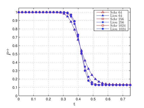
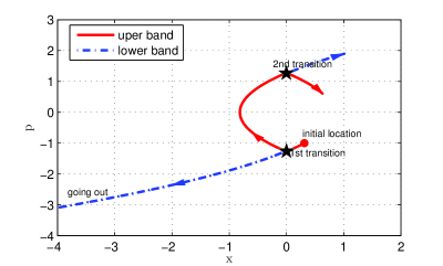
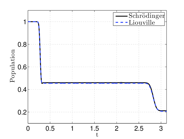
The evolution of the particle wave packets can be easily understood. The trajectories of the wave packets center-of-mass are illustrated in Figure 4.1. The Gaussian profile has a negative mean velocity and passes through the crossing point $x=0$ at around $t=0.25$. The Gaussian wave function splits into two parts. Around one half of the particles enter into the lower energy band, and the others stay in the upper band. The packet on the lower energy level is accelerated and leaves the simulation domain. The particles on the higher energy band are accelerated on the opposite direction, the momentum decreases and the wave packet is reflected around $x=-1$. At $t=2.75$, the wave passes through the crossing point for the second time, and undergoes another hopping process. In Figure 4.2 we show the evolution of $P^{+}$ with respect to time. As the wave packet passes through the crossing point twice, the mass gets transferred to another energy band twice, generating two jumps in $P^{+}$. The numerical results given by the semiclassical model shows good agreement with that of the Schrödingier equation.

Figure 4.1: The trajectories of wave packets: initially, the wave packet centers around the bullet point and starts moving towards the crossing point at $x=0$, marked as a star. It splits into two parts there: one of them, denoted by the dash-point line, keeps moving towards the left, while the other wave packet, the one that jumps up to the higher energy band, bounces back and hits the origin at $x=0$. Over there, it goes through the “second transition” and splits up into trajectories.

Figure 4.2: Time evolution of $P^{+}$ (4.4).

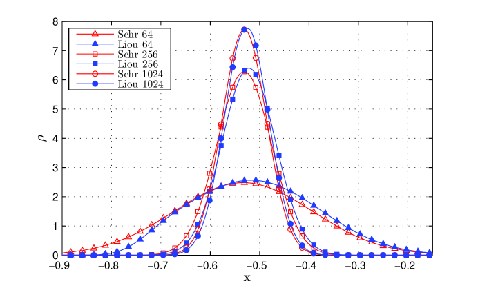
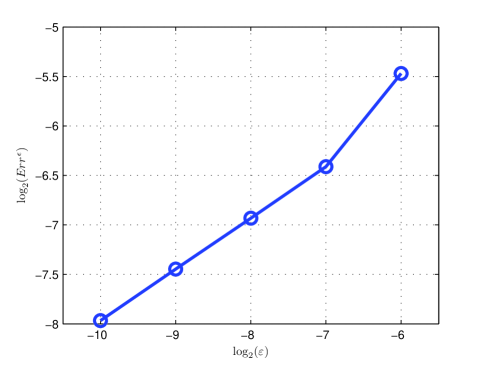
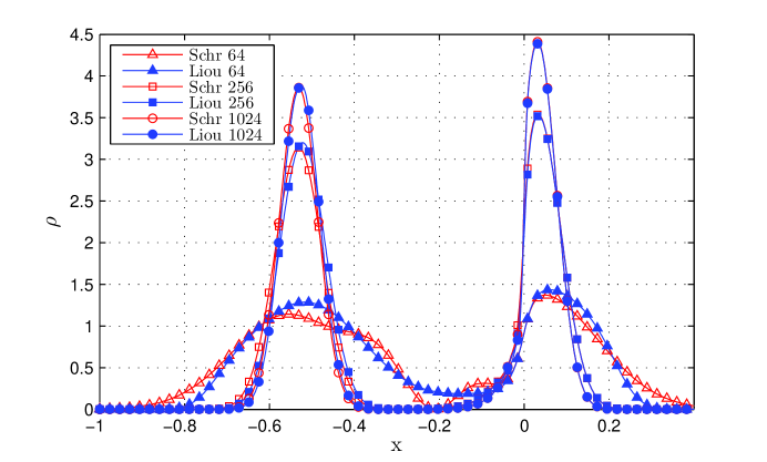
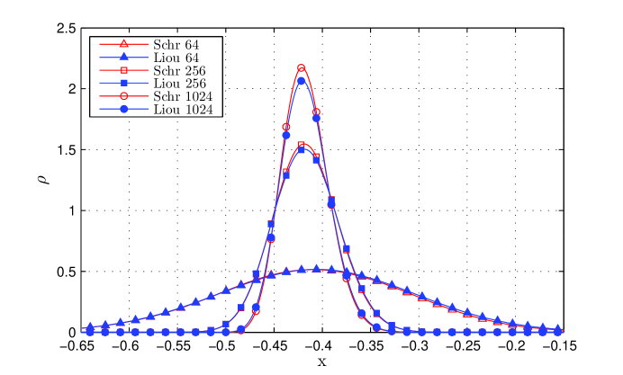
We compare the results of our model with that of the Schrödinger. In Figure 4.3 we compare the results $\rho^{\pm}$ given by the two systems at time $t=0.75$ ($a^{+}=1$, $a^{-}=0$, $x_{0}=0.5$, and $p_{0}=-1$). In Figure 4.4 we check the evolution of the population on the first band $P^{+}$ along the time. Figure 4.5 shows that the hybrid model error (4.6) decreases at the rate of $\mathcal{O}(\sqrt{\varepsilon})$ for $\delta=\mathcal{O}(\sqrt{\varepsilon})$. The simulations show a good agreement between the two system.

(a) $\rho^{+}_{schr/liou}$

(b) $\rho^{-}_{schr/liou}$

Figure 4.3: One dimensional system simulation: the density functions $\rho^{\pm}_{schr/liou}$ for different $\varepsilon$ at time $t=0.75$, $\delta=\sqrt{\varepsilon}/4$. The legend “Schr $n$” (or “Liou $n$”) represents the solution of the Schrödinger equation (or the hybrid model) with $\varepsilon=1/n$. Here, $a^{+}=1$, $a^{-}=0$, $x_{0}=0.5$, and $p_{0}=-1$.

Figure 4.4: One dimensional system simulation: time evolution of the population on the upper band $P^{+}_{schr/liou}$ with $\delta=\sqrt{\varepsilon}/4$. The legend “Schr $n$” (or “Liou $n$”) represents the solution of the Schödinger equation (or the hybrid model) with $\varepsilon=1/n$. Here, $a^{+}=1$, $a^{-}=0$, $x_{0}=0.5$, and $p_{0}=-1$.

Figure 4.5: One dimensional system simulation: $\text{Err}^{\varepsilon}$ (4.6) decreases with a rate of $O(\sqrt{\varepsilon})$. Here, $a^{+}=1$, $a^{-}=0$, $x_{0}=0.5$, $p_{0}=-1$, and $t=0.75$.

We consider now a different initial condition. The initial wave packet for the Schrödinger equation is now given by (4.1)-(4.2) with $a^{+}=a^{-}=1/\sqrt{2}$, $x_{0}=0.5$, and $p_{0}=-1$. This initial datum corresponds to a linear superposition of two Gaussian packets that belong to the upper and lower bands respectively.

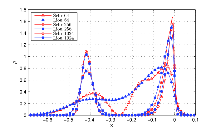
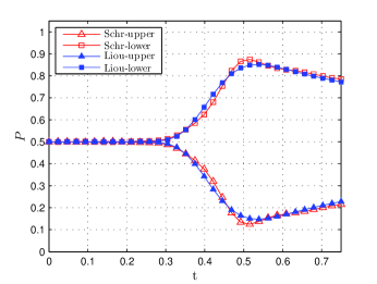
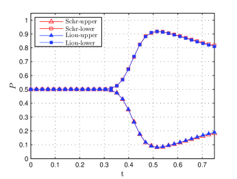
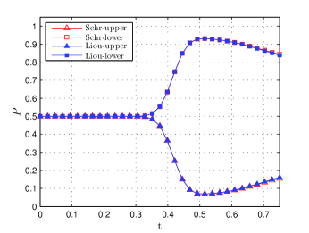
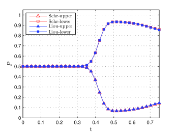
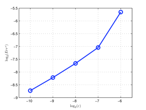
In Figure 4.6 we compare the numerical results of $\rho^{\pm}$ to the Schrödinger equation and those to (2.17) for $t=0.75$. In Figure 4.7, we show the evolution of the populations on the upper and lower bands $P^{\pm}$ with respect to time. We see that in the case of large $\varepsilon$ the semiclassical solution is not completely satisfactory. However it is able to capture the main structure of the quantum interference between the upper and the lower band waves. For small $\varepsilon$, the two wave packets are well-separated, the solution of the hybrid model is in good agreement with the Schrödinger solution. Figure 4.8 shows that the cumulative error decreases at the rate of $\mathcal{O}(\sqrt{\varepsilon})$.

(a) $\rho^{+}_{schr/liou}$

(b) $\rho^{-}_{schr/liou}$

Figure 4.6: One dimensional system simulation: the density functions $\rho^{\pm}_{schr/liou}$ for different $\varepsilon$ at time $t=0.75$, $\delta=\sqrt{\varepsilon}/4$. The legend “Schr $n$” (or “Liou $n$”) represents the solution of the Schödinger equation (or the hybrid model) with $\varepsilon=1/n$. Here, $a^{+}=a^{-}=1/\sqrt{2}$, $x_{0}=0.5$, and $p_{0}=-1$.

(a) $\varepsilon=2^{-6}$

(b) $\varepsilon=2^{-7}$

(c) $\varepsilon=2^{-8}$

(d) $\varepsilon=2^{-9}$

Figure 4.7: One dimensional system simulation: time evolution of the population on the upper and lower bands $P^{\pm}_{schr/liou}$ (4.4). $\delta=\sqrt{\varepsilon}/4$. The legend “Schr-upper” ( or “Schr-lower”) represents the population on upper (or lower) band given by the Schrödinger equation, “Liou-upper” ( or “Liou-lower”) represents the population on upper (or lower) band given by the hybrid model. Here, $a^{+}=a^{-}=1/\sqrt{2}$, $x_{0}=0.5$, and $p_{0}=-1$.

Figure 4.8: One dimensional system simulation: $\text{Err}^{\varepsilon}$ (4.6) as a function of $\varepsilon$ at $t=0.75$. Here, $a^{+}=a^{-}=1/\sqrt{2}$, $x_{0}=0.5$, and $p_{0}=-1$.

4.2 Two-dimensional system

In this example, we deal with the problem in 2D with a pure state initial data. We set $u$ and $v$ as

$$u(x)=x,\quad\text{and}\quad v(x)=\sqrt{y^{2}+\delta^{2}}.$$

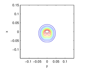
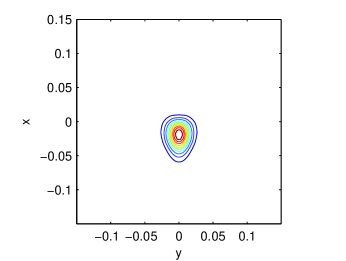
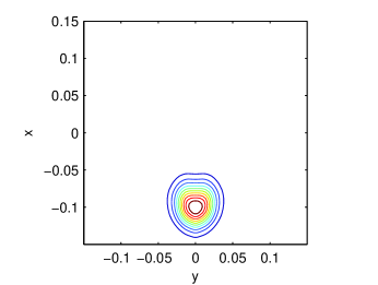
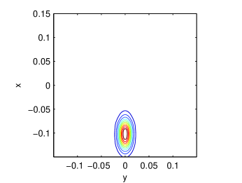
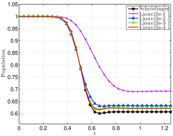
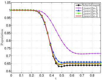
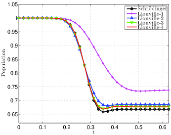
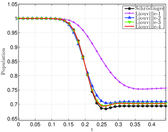
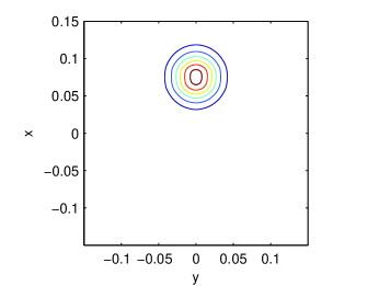
We choose $\delta=\sqrt{\varepsilon}/2$. The minimum of energy gap is $2\delta$ and is located at the origin of the axis. The initial data for the Schrödinger equation are given in (4.1)-(4.2) with $a^{+}=1$, $a^{-}=0$, $x_{0}=5\sqrt{\varepsilon}$, $y_{0}=0$, ${p_{0}}_{x}=-1$, and ${p_{0}}_{y}=0$. The Schrödinger equation is computed using the classical time-splitting spectral method, with $\Delta x=\Delta y=\varepsilon/8$ and $\Delta t=5\varepsilon^{\frac{3}{2}}$ and the hybrid model is computed with $\Delta x=\Delta p=h$ in the adiabatic regions and $\Delta x=\Delta p=h/2$ in the non-adiabatic region, where $h=O(\sqrt{\varepsilon})$. In Figure 4.9 we show the snapshots of the density contour computed by the semiclassical model, while in Figure 4.10 we compare the evolution of the population on the first band $P^{+}$ along the time given by the two systems. In Figure 4.9 we see that as time passes by, the density from the first band has some proportion jumping up to the second one. In Figure 4.10 we can clearly see that with resolved mesh the numerical solution to the semiclassical model agrees with that given by the Schrödinger equation.

(a) $t=0.0781$

(b) $t=0.1562$

(c) $t=0.2344$

Figure 4.9: Two dimensional system simulation: the time evolution of density contour computed by the hybrid model. The left/right column are for $\rho^{+}_{liou}$/ $\rho^{-}_{liou}$, the density on the upper/lower band (4.4). $\delta=\sqrt{\varepsilon}/2$ and $\varepsilon=2^{-10}$. One can see in (b) around time $t=0.1562$, the wave packet hits the crossing point and a portion of the mass jumps to the upper band.

(a) $\varepsilon=2^{-6}$

(b) $\varepsilon=2^{-7}$

(c) $\varepsilon=2^{-8}$

(d) $\varepsilon=2^{-9}$

Figure 4.10: Two dimensional system simulation: time evolution of the population on the upper band $P^{+}_{schr/liou}$ (4.4). $\delta=\sqrt{\varepsilon}/2$. The legend “Schrödinger” represents the solution of the Schrödinger equation, “Liouville-$j$” represents the solution of the hybrid model with $\Delta x=\Delta p=h$ in the adiabatic regions and $\Delta x=\Delta p=h/2$ in the non-adiabatic region, where $h=\sqrt{\varepsilon}/2^{j-1}$, and $j=1,2,3,4$.

5 Conclusion

In conclusion, we derived a semiclassical model for the non-adiabatic transition between different potential energy surfaces that goes beyond the classical Born-Oppenheimer approximation. By considering the complete Wigner matrix including the off-diagonal terms, our model is able to capture interesting physical phenomena such as the band-to-band transition, and the quantum correlation induced by the Berry connection. The hybrid model we proposed combines the classical adiabatic limit and the semiclassical model together to reduce the computational cost. The numerical simulations show that the hybrid model has a good agreement with the full quantum simulation.

Appendix: The Derivation of the Hamiltonian ${H^{\prime}}$

We give some details concerning the computation of the ${H}$’ of Eq. (2.16). From the definition of $\mathcal{H}$’ we have

$$H^{\prime} = \Theta(\boldsymbol{x})\#H(\boldsymbol{x},\boldsymbol{p})\#\Theta^{\dagger}(\boldsymbol{x})$$ (5.1)

$$= \Theta(\boldsymbol{x})\#\big{(}U(\boldsymbol{x})\mathbb{I}+V(\boldsymbol{x})\big{)}\#\Theta^{\dagger}(\boldsymbol{x})+\Theta(\boldsymbol{x})\#\left(\frac{\boldsymbol{p}^{2}}{2}\mathbb{I}\right)\#\Theta^{\dagger}(\boldsymbol{x})$$

$$= \mathrm{diag}\left\{U+E,\,U-E\right\}\,+\,\Theta(\boldsymbol{x})\#\left(\frac{\boldsymbol{p}^{2}}{2}\mathbb{I}\right)\#\Theta^{\dagger}(\boldsymbol{x})$$

$$= \Lambda(\boldsymbol{x},\boldsymbol{p})+\mathrm{i}\varepsilon\boldsymbol{p}\cdot\nabla_{\boldsymbol{x}}\Theta(\boldsymbol{x})\Theta^{\dagger}(\boldsymbol{x})+\frac{\varepsilon^{2}}{2}\nabla_{\boldsymbol{x}}\Theta(\boldsymbol{x})\cdot\nabla_{\boldsymbol{x}}\Theta^{\dagger}(\boldsymbol{x}),$$

where $\Lambda=U(\boldsymbol{x})+\Lambda_{V}$ with $\Lambda_{V}$ defined in (1.7) and we used the first order expansion of the Moyal product

$$A\#B = \sum_{n}\frac{1}{n!}\left(\frac{\mathrm{i}\varepsilon}{2}\right)^{n}A\left(\overleftarrow{\nabla_{\boldsymbol{x}}}\cdot\overrightarrow{\nabla_{\boldsymbol{p}}}-\overleftarrow{\nabla_{\boldsymbol{p}}}\cdot\overrightarrow{\nabla_{\boldsymbol{x}}}\right)^{n}B$$

$$= AB+\frac{\mathrm{i}\varepsilon}{2}\left(\nabla_{\boldsymbol{x}}A\cdot\nabla_{\boldsymbol{p}}B-\nabla_{\boldsymbol{p}}A\cdot\nabla_{\boldsymbol{x}}B\right)+o(\varepsilon).$$

In particular, we used

$$\Theta(\boldsymbol{x})\#\left(\frac{\boldsymbol{p}^{2}}{2}\mathbb{I}\right) = \frac{\boldsymbol{p}^{2}}{2}\Theta+\frac{\mathrm{i}\varepsilon}{2}\boldsymbol{p}\cdot\nabla_{\boldsymbol{x}}\Theta+\frac{1}{2}\left(\frac{\mathrm{i}\varepsilon}{2}\right)^{2}\Theta\left(\overleftarrow{\nabla_{\boldsymbol{x}}}\cdot\overrightarrow{\nabla_{\boldsymbol{p}}}\right)^{2}\left(\frac{\boldsymbol{p}^{2}}{2}\mathbb{I}\right)+o(\varepsilon^{2})$$

$$= \frac{\boldsymbol{p}^{2}}{2}\Theta+\frac{\mathrm{i}\varepsilon}{2}\boldsymbol{p}\cdot\nabla_{\boldsymbol{x}}\Theta+\frac{1}{2}\left(\frac{\mathrm{i}\varepsilon}{2}\right)^{2}\Delta_{\boldsymbol{x}}\Theta+o(\varepsilon^{2}),]$$

and

$$\left(\frac{\boldsymbol{p}^{2}}{2}\Theta(\boldsymbol{x})\right)\#\Theta^{\dagger}(\boldsymbol{x}) = \frac{\boldsymbol{p}^{2}}{2}-\frac{\mathrm{i}\varepsilon}{2}\Theta\,(\boldsymbol{p}\cdot\nabla_{\boldsymbol{x}}\Theta^{\dagger})+\frac{1}{2}\left(\frac{\mathrm{i}\varepsilon}{2}\right)^{2}\Theta\,\Delta_{\boldsymbol{x}}\Theta^{\dagger},$$

$$\big{(}\boldsymbol{p}\cdot\nabla_{\boldsymbol{x}}\Theta(\boldsymbol{x})\big{)}\#\Theta^{\dagger}(\boldsymbol{x}) = \boldsymbol{p}\cdot\nabla_{\boldsymbol{x}}\Theta\,\Theta^{\dagger}-\frac{\mathrm{i}\varepsilon}{2}\nabla_{\boldsymbol{x}}\Theta\cdot\nabla_{\boldsymbol{x}}\Theta^{\dagger},$$

$$\Delta_{\boldsymbol{x}}\Theta(\boldsymbol{x})\#\Theta^{\dagger}(\boldsymbol{x}) = \Delta_{\boldsymbol{x}}\Theta\,\Theta^{\dagger},$$

$$\Theta(\boldsymbol{x})\,(\boldsymbol{p}\cdot\nabla_{\boldsymbol{x}}\Theta^{\dagger}(\boldsymbol{x})) = -(\boldsymbol{p}\cdot\nabla_{\boldsymbol{x}}\Theta)\,\Theta^{\dagger},$$

$$-2\nabla_{\boldsymbol{x}}\Theta(\boldsymbol{x})\cdot\nabla_{\boldsymbol{x}}\Theta^{\dagger}(\boldsymbol{x}) = \Theta\Delta_{\boldsymbol{x}}\Theta^{\dagger}+\Delta_{\boldsymbol{x}}\Theta\,\Theta^{\dagger}.$$

References

• [1] J. E. Avron and A. Elgart. Adiabatic theorem without a gap condition: Two-level system coupled to quantized radiation field. Physical Review A, 58(6):4300, 1998.
• [2] W. Bao, S. Jin, and P. A. Markowich. On time-splitting spectral approximations for the schrödinger equation in the semiclassical regime. Journal of Computational Physics, 175(2):487–524, January 2002.
• [3] D. R. Bates. Collisions involving the crossing of potential energy curves. Proceedings of the Royal Society of London. Series A, Mathematical and Physical Sciences, 257(1288):22–31, 1960.
• [4] A. Böhm, A. Mostafazadeh, H. Koizumi, Q. Niu, and J. Zwanziger. The geometric phase in quantum systems: foundations, mathematical concepts, and applications in molecular and condensed matter physics. Springer, 2003.
• [5] M. Born and R. Oppenheimer. Zur quantentheorie der molekeln [on the quantum theory of molecules]. Annalen der Physik (in German), 389(20):457–484, 1927.
• [6] R. Bourquin, V. Gradinaru, and G. A. Hagedorn. Non-adiabatic transitions near avoided crossings: theory and numerics. Journal of Mathematical Chemistry, 50(3):602–619, May 2011.
• [7] L. Chai, S. Jin, and Q. Li. Semi-classical models for the schrödinger equation with periodic potentials and band crossings. Kinetic and Related Models, 6(3):505–532, May 2013.
• [8] C. Fermanian Kammerer and C. Lasser. Wigner measures and codimension two crossings. Journal of Mathematical Physics, 44(2):507–557, 2003.
• [9] C. Fermanian-Kammerer and C. Lasser. Single switch surface hopping for molecular quantum dynamics. Journal of Mathematical Chemistry, 50(3):620–635, April 2011.
• [10] P. Gérard, P. A. Markowich, N. J. Mauser, and F. Poupaud. Homogenization limits and wigner transforms. Communications on Pure and Applied Mathematics, 50(4):323–379, 1997.
• [11] L. Gosse and P. A. Markowich. Multiphase semiclassical approximation of an electron in a one-dimensional crystalline lattice. Journal of Computational Physics, 197(2):387–417, July 2004.
• [12] G. A. Hagedorn and A. Joye. Mathematical analysis of born-oppenheimer approximations. In F. Gesztesy, P. Deift, C. Galvez, P. Perry, and W. Schlag, editors, Spectral Theory and Mathematical Physics, page 203, 2007.
• [13] G. A. Hagedorn. A time dependent born-oppenheimer approximation. Communications in Mathematical Physics, 77(1):1–19, 1980.
• [14] G. A. Hagedorn. High order corrections to the time-dependent born-oppenheimer approximation i: Smooth potentials. Annals of Mathematics, 124(3):pp. 571–590, 1986.
• [15] G. A. Hagedorn. High order corrections to the time-dependent born-oppenheimer approximation. II: coulomb systems. Communications in mathematical physics, 117(3):387–403, 1988.
• [16] G. A. Hagedorn. Proof of the Landau-Zener formula in an adiabatic limit with small eigenvalue gaps. Communications in mathematical physics, 136(3):433–449, 1991.
• [17] G. A. Hagedorn. Classification and normal forms for avoided crossings of quantum-mechanical energy levels. Journal of Physics A: Mathematical and General, 31(1):369–383, 1998.
• [18] G. A. Hagedorn and A. Joye. Landau-Zener transitions through small electronic eigenvalue gaps in the born-oppenheimer approximation. In Annales de l’Institut Henri Poincare-A Physique Theorique, volume 68, page 85, 1998.
• [19] G. A. Hagedorn and A. Joye. Molecular propagation through small avoided crossings of electron energy levels. Reviews in Mathematical Physics, 11(01):41–101, 1999.
• [20] G. A. Hagedorn and A. Joye. A time-dependent Born-Oppenheimer approximation with exponentially small error estimates. Communications in Mathematical Physics, 223(3):583–626, 2001.
• [21] M. F. Herman. Generalization of the geometric optical series approach for nonadiabatic scattering problems. The Journal of Chemical Physics, 76(6):2949, 1982.
• [22] L. Hörmander. The Weyl calculus of pseudo-differential operators. Communications on Pure and Applied Mathematics, 32(3):359–443, 1979.
• [23] V. Jakšić and J. Segert. On the Landau–Zener formula for two-level systems. Journal of Mathematical Physics, 34(7):2807, 1993.
• [24] S. Jin and P. Qi. A hybrid Schrödinger/Gaussian beam solver for quantum barriers and surface hopping. Kinetic and Related Models, 4(4):1097–1120, 2011.
• [25] S. Jin, P. Qi, and Z. Zhang. An Eulerian surface hopping method for the Schrödinger equation with conical crossings. Multiscale Modeling & Simulation, 9(1):258–281, January 2011.
• [26] S. Jin and D. Yin. Computational high frequency waves through curved interfaces via the Liouville equation and geometric theory of diffraction. Journal of Computational Physics, 227(12):6106–6139, June 2008.
• [27] A. Joye, H. Kunz, and C.-E. Pfister. Exponential decay and geometric aspect of transition probabilities in the adiabatic limit. Annals of Physics, 208(2):299 – 332, 1991.
• [28] A. Joye and C.-E. Pfister. Exponentially small adiabatic invariant for the Schrödinger equation. Communications in Mathematical Physics, 140(1):15–41, 1991.
• [29] R. Kapral and G. Ciccotti. Mixed quantum-classical dynamics. The Journal of Chemical Physics, 110(18):8919, 1999.
• [30] T. Kato. On the adiabatic theorem of quantum mechanics. Journal of the Physical Society of Japan, 5(6):435–439, November 1950.
• [31] C. Lasser, T. Swart, and S. Teufel. Construction and validation of a rigorous surface hopping algorithm for conical crossings. Communications in Mathematical Sciences, 5(4):789–814, 2007.
• [32] R. J. LeVeque. Numerical methods for conservation laws, volume 132. Springer, 1992.
• [33] P. Lions and T. Paul. Sur les mesures de Wigner. Rev. Mat. Iberoamericana, 9(3):553–618, 1993.
• [34] O. Morandi. Effective classical liouville-like evolution equation for the quantum phase-space dynamics. Journal of Physics A: Mathematical and Theoretical, 43(36):365302, 2010.
• [35] O. Morandi and F. Schürrer. Wigner model for quantum transport in graphene. Journal of Physics A: Mathematical and Theoretical, 44(26):265–301, July 2011.
• [36] O. Morandi. Multiband wigner-function formalism applied to the zener band transition in a semiconductor. Physical Review B, 80(2):024301, 2009.
• [37] O. Morandi and F. Schürrer. Wigner model for klein tunneling in graphene. Communications in Applied and Industrial Mathematics, 2(1), 2011.
• [38] G. Nenciu and V. Sordoni. Semiclassical limit for multistate Klein-Gordon systems: almost invariant subspaces, and scattering theory. Journal of Mathematical Physics, 45(9):3676–3696, 2004.
• [39] G. Panati, H. Spohn, and S. Teufel. Space-adiabatic perturbation theory in quantum dynamics. Physical Review Letters, 88(25):205405, June 2002.
• [40] V. Rousse. Landau-Zener transitions for eigenvalue avoided crossings in the adiabatic and Born-Oppenheimer approsimations. Asymptotic Analysis, 37(3):293–328, 2004.
• [41] H. Spohn and S. Teufel. Adiabatic decoupling and time-dependent Born-Oppenheimer theory. Communications in Mathematical Physics, 224(1):113–132, 2001.
• [42] S. Teufel. Adiabatic Perturbation Theory in Quantum Dynamics. Springer, 2003.
• [43] J. C. Tully. Trajectory surface hopping approach to nonadiabatic molecular collisions: The reaction of H+superscriptH\mathrm{H}^{+} with D2subscriptD2\mathrm{D}_{2}. The Journal of Chemical Physics, 55(2):562–572, 1971.
• [44] J. C. Tully. Molecular dynamics with electronic transitions. The Journal of Chemical Physics, 93(2):1061–1071, 1990.
• [45] J. von Neuman and E. Wigner. Uber merkwürdige diskrete eigenwerte. uber das verhalten von eigenwerten bei adiabatischen prozessen. Zhurnal Physik, 30:467–470, 1929.
• [46] H. Weyl. Quantenmechanik und gruppentheorie. Zeitschrift für Physik, 46(1-2):1–46, 1927.
• [47] G. A. Worth and L. S. Cederbaum. Beyond Born-Oppenhermer: molecular dynamics through a conical intersection. Annual Review of Physical Chemistry, 55(1):127–158, June 2004.
• [48] D. Xiao, M. Chang, and Q. Niu. Berry phase effects on electronic properties. Reviews of Modern Physics, 82(3):1959–2007, 2010.
• [49] D. R. Yarkony. Nonadiabatic quantum Chemistry-Past, present, and future. Chemical Reviews, 112(1):481–498, January 2012.
• [50] C. Zener. Non-adiabatic crossing of energy levels. Proceedings of the Royal Society of London. Series A, Containing Papers of a Mathematical and Physical Character, 137(833):696–702, 1932.