Holographic reconstruction of $f(G)$ Gravity for scale factors pertaining to Emergent, Logamediate and Intermediate scenarios

Abstract

In this paper, we reconstruct the holographic dark energy in the framework of $f(G)$ modified theory of gravity, where $G$ is Gauss-Bonnet invariant. In this context, we choose the infrared cut-off as Granda-Oliveros cut-off which is proportional to the Hubble parameter $H$ and its first derivative with respect to the cosmic time $t$. We reconstruct $f(G)$ model with the inclusion of HDE and three well-known forms of the scale factor $a(t)$, i.e. the emergent, the logamediate and the intermediate scale factors. The reconstructed model as well as equation of state parameter are discussed numerically with the help of graphical representation to explore the accelerated expansion of the universe. Moreover, the stability of the models incorporating all the scale factors is checked through squared speed of sound $v_{s}^{2}$.

I Introduction

It is established by cosmological observations (e.g. SNe Ia, CMB) that the present universe is undergoing a phase of accelerated expansion 24 ; 32 . The physical origin of this cosmic acceleration has continued to be a deep mystery till date. Two approaches have been adopted to explain this accelerated expansion. They are:

1. To introduce “dark energy” (DE) in the right-hand side of the Einstein equation in the framework of general relativity (recent reviews include 8 ; 9 ; 27 ; 1 );

2. To introduce “modified theory of gravity” by modifing the left-hand side of the Einstein equation (recent reviews include 22 ; 18 ; 21 ).

In an exhaustive review, Clifton et al. 7 has thoroughly discussed the motivations behind modified gravity theory. In Nojiri and Odintsov 19 , a detailed account of the advantages of the modified gravity has been presented. According to Nojiri and Odintsov 19 , some significant advantages of modified gravity theory are:

• Modified gravity provides the very natural gravitational alternative for dark energy;

• Modified gravity presents very natural unification of the early-time inflation and late-time acceleration;

• Modified gravity serves as the basis for unified explanation of dark energy and dark matter;

• Modified gravity describes the transition from deceleration to acceleration in the universe evolution.

The development in the study of black hole theory and string theory results the holographic principle 4 . The holographic principle “calls into question not only the fundamental status of field theory but the very notion of locality” 4 . The Holographic DE (HDE), based on the holographic principle, is one of the most studied models of DE 15 ; 11 ; 10 ; 12 . The present work is devoted to the holographic reconstruction of one kind of modified gravity theory, namely $f(G)$, via three choices to scale factor pertaining to emergent, logamediate and intermediate scenarios respectively. Thus, a three layered discussion would be presented in the subsequent portion of this Section. Firstly, we survey the choices of the scale factor. Choices of scale factors for the scenarios mentioned above are:

1. Emergent scenario 17 , where the scale factor has the form $a(t)=A\left(B+e^{nt}\right)^{\beta}$ with $A>0,~{}B>0,~{}n>0,~{}\beta>1$.

2. Intermediate scenario 2 ; 3 , where $a(t)=\exp\left[Bt^{\beta}\right]$ with $B>0,~{}0<\beta<1$.

3. Logamediate scenario 2 , where $a(t)=\exp\left[B(\ln t)^{\beta}\right]$ with $B>0,~{}\beta>1$.
   

Since reconstruction of a modified gravity is the basic purpose of the present work, we now review the current status of research in this direction. Reconstruction of DE has been addressed by a number of researchers. Important references in this direction include 26 ; 28 ; 6 ; 16 . Setare and Saridakis 30 considered the holographic and Gauss-Bonnet DE models separately to investigate the conditions under which these models can be simultaneously valid. This correspondence leads to accelerated expansion of the universe. The same authors 31 discussed the correspondence of HDE model with canonical, phantom and quintom models minimally coupled to gravity and observed consistent results about acceleration of the universe. Chattopadhyay and Pasqua 5 developed the correspondence between $f(T)$ gravity and HDE model and discussed the accelerated expansion of the universe. Jawad et al. 13 reconstructed the HDE model in context of $f(G)$ gravity with a power-law solution. They found analytical solution for $f(G)$ model in this scenario to discuss the EoS parameter, the stability analysis as well as energy conditions to explore the current expansion of the universe.

Motivated by these works, we have developed the reconstructed scenario of HDE model with $f(G)$ model for three different scale factors to represent a variety of models to discuss the accelerated expansion of the universe. We have just extended our works 5 ; 13 , reconstructing HDE model with GO cut-off in the frame of $f(G)$ modified theory of gravity for a variety of scale factors (i.e. the emergent, the logamediate and the intermediate one). We draw the numerically solution of the reconstructed scenario with the help of three different forms of scale factors. The paper is organized as follows: In the next section, we provide formalism of $f(G)$ gravity and HDE model. Section III is devoted to the brief discussion of scale factors. The reconstructed scenario via scale factors is given in section IV. The last section contains the concluding remarks.

II Brief overview of $f(G)$ gravity and HDE

In this Section, we will describe some important features of $f(G)$ gravity and establish a correspondence between $f(G)$ and HDE. For this purpose, we consider an action representing a special form of $f(G)$ gravity model which contains an Einstein gravity term with perfect fluid and an arbitrary function of Gauss-Bonnet term 25 . The action $S$ of this $f(G)$ modified gravity is given by

$$S=\int d^{4}x\sqrt{-g}\left[\frac{1}{2\kappa^{2}}R+f(G)+\mathcal{L}_{m}\right],$$ (1)

where $G=R^{2}-4R_{\mu\nu}R^{\mu\nu}+R_{\mu\nu\lambda\sigma}R^{\mu\nu\lambda\sigma}$ (with $R$ representing the Ricci scalar curvature, $R_{\mu\nu}$ is the Ricci curvature tensor and $R_{\mu\nu\lambda\sigma}$ denotes the Riemann curvature tensor), $\kappa^{2}=8\pi G_{N}$ (with $G_{N}$ being the gravitational constant), $g$ represents the determinant of the metric tensor $g_{\mu\nu}$ and $\mathcal{L}_{m}$ represents the Lagrangian of the matter present in the universe. The variation of $S$ with respect to the metric tensor $g_{\mu\nu}$ generates the field equations. For spatially flat FRW metric, the Ricci scalar curvature $R$ and the Gauss-Bonnet invariant $G$, take the following expressions respectively

$$R=6(\dot{H}+2H^{2}),\quad G=24H^{2}(\dot{H}+H^{2}),$$ (2)

where the upper dot represents the derivative with respect to the cosmic time $t$.

The first FRW equation (with $8\pi G_{N}=1)$ takes the form

$$H^{2}=\frac{1}{3}\left[Gf_{G}-f(G)-24\dot{G}H^{3}f_{GG}+\rho_{m}\right]=\frac{1}{3}\left(\rho_{G}+\rho_{m}\right),$$ (3)

where $f_{G}$ and $f_{GG}$ represents, respectively, the first and the second derivative of $f$ with respect to $G$, i.e. $f_{G}=\frac{df}{dG}$ and $f_{GG}=\frac{d^{2}f}{dG^{2}}$. Setare 29 has recently reconstructed $f(R)$ modified gravity from HDE with IR cutoff as event horizon. Here we discuss a reconstruction scheme of the above form of $f(G)$ gravity in HDE framework taking Granda-Oliveros cut-off. The HDE density is defined as 29

$$\rho_{\Lambda}=\frac{3}{L_{GO}^{2}},$$ (4)

where $L_{GO}$ represents the Granda-Oliveros cut-off, which is defined as

$$L_{GO}=\left(\lambda H^{2}+\delta\dot{H}\right)^{-\frac{1}{2}},$$ (5)

where $\lambda$ and $\delta$ are constants. The dimensionless DE density is obtained by dividing the energy density $\rho_{\Lambda}$ of DE with the critical energy density $\rho_{cr}=3H^{2}$, yields

$$\Omega_{\Lambda}=\frac{\rho_{\Lambda}}{\rho_{cr}}=\frac{c^{2}}{L_{GO}^{2}H^{2}}.$$ (6)

Moreover, we define the EoS parameter $\omega_{eff}$ is defined as:

$$\omega_{eff}=\frac{p_{eff}}{\rho_{eff}},$$ (7)

where

$$\rho_{eff} = \rho+\frac{1}{2\kappa^{2}}\left[-f\left(G\right)+24H^{2}\left(H^{2}+\dot{H}\right)f^{\prime}\left(G\right)\right],$$ (8)

$$p_{eff} = p+\frac{1}{2\kappa^{2}}\left\{f\left(G\right)-24H^{2}\left(H^{2}+\dot{H}\right)f^{\prime}\left(G\right)+(24)8H^{2}\left[6\dot{H}^{3}+6H\dot{H}\ddot{H}+24H^{2}\dot{H}^{2}\right.\right.$$

$$+ \left.\left.6H^{3}\ddot{H}+8H^{4}\dot{H}+H^{2}\dddot{H}\right]f^{\prime\prime}\left(G\right)+(24^{2})8H^{4}\left(2H^{2}+H\ddot{H}+4H^{2}\dot{H}\right)^{2}f^{\prime\prime\prime}\left(G\right)\right\}.$$

The prime denotes the derivative of the function with respect to $G$.

III Discussion on the various scale factors

Now we provide a glimpse on the main features of three scale factors considered (i.e. the emergent, the logamediate and the intermediate ones) and derive some related physical quantities from them to discuss the reconstructed scenario.

III.1 Emergent Scale Factor

The emergent scale factor is given by 17

$$a(t)=A\left[B+\exp(nt)\right]^{\beta},$$ (10)

where $A,~{}B,~{}n$ and $\beta$ are positive constants. The avoid any singularity, we have to take $B>0$ whereas $A$ should be greater than zero for the positivity of scale factor. For $a<0$ or $\beta<0$, the universe bears a big bang singularity, so for the expanding model $a>0$ or $\beta>0$. This kind of scale factor was recently used by Mukherjee et al. 17 and Paul and Ghose 23 . The Hubble parameter and the Gauss-Bonnet invariant $G$, taking into account the scale factor (10), are given, respectively, by

$$H=\frac{n\beta\exp(nt)}{B+\exp(nt)},\quad G=\frac{24n^{4}\beta^{3}\exp(3nt)\left[B+\beta\exp(nt)\right]}{\left[B+\exp(nt)\right]^{4}}.$$ (11)

III.2 Logamediate

The next scale factor considered is the logamediate one, which has the form 2 ; 3

$$a(t)=\exp\left[B(\ln t)^{\beta}\right],$$ (12)

where $B\beta>0$ and $\beta>1$. Barrow and Nunes 3 studied the logamediate inflation, where the scale factor expands just the logamediate scale factor expressed here. In this case, $H$ and $G$ take the form

$$H=\frac{B\beta\log\left(t\right)^{\beta-1}}{t},\quad G=\frac{24B^{3}\beta^{3}\log\left(t\right)^{3\beta-4}\left[B\beta\log\left(t\right)^{\beta}-\log\left(t\right)+\beta-1\right]}{t^{4}}.$$ (13)

III.3 Intermediate

The intermediate scale factor is given by 2

$$a(t)=\exp\left[Bt^{\beta}\right],$$ (14)

where $B>0$ and $0<\beta<1$. This kind of scale factor was used in the work of Khatua and Debnath 14 . In this case, the Hubble parameter $H$ is given by

$$H=B\beta t^{\beta-1}.$$ (15)

Moreover, $G$ can be written as

$$G=24B^{3}\beta^{3}t^{3\beta-4}\left(B\beta t^{\beta}+\beta-1\right)$$ (16)

IV Holographic reconstruction of $f(G)$ gravity

In this Section, we discuss the HDE reconstruction of $f(G)$ gravity with the help of three scale factors considered. In order to incorporate the correspondence, we equate the energy density $\rho_{G}$ of $f(G)$ gravity (given in Eq.(3)) and energy density $\rho_{\Lambda}$ of HDE model (given in Eq.(4)), which leads to the following differential equation 19 ; 20

$$24H^{3}\dot{G}^{-1}\ddot{f}(G)-(24H^{3}\dot{G}^{-2}\ddot{G}-G\dot{G}^{-1})\dot{f}(G)+f(G)=-3(\delta\dot{H}+\lambda H^{2}).$$ (17)

The search for analytical solution of this differential equation is very difficult. Thus, we prefer the numerical solutions of this equation for $f(G)$ to elaborate the behavior of EoS parameter and squared speed of sound $v_{s}^{2}$ in reconstructed scenario of HDE in the framework of $f(G)$ gravity.

IV.1 For Emergent Scale Factor

We plot the $f(G)$ model of gravity obtained numerically against the cosmic $t$ for the emergent scale factor taking three different values of $\beta$ (i.e. 1.2, 1.4 and 1.6) as shown in Figure 1. We also use the following values for the remaining constants of the scale factor: $A=2,~{}B=3.5,~{}n=4.5$ while $\lambda=1.5,~{}\delta=1$ for the new HDE model. Initially, the graph shows a negatively increasing behavior of $f(G)$ with respect to the cosmic time $t$. Afterwards, it converges to zero as the time passes for all considered values of $\beta$. Figure 2 represents the graph of the squared speed of sound $v_{s}^{2}$ against the cosmic time $t$ considering the same values of constants given above. For this quantity, we use the expression $v_{s}^{2}=\frac{\dot{p}_{eff}}{\dot{\rho}_{eff}}$ along with Eq. (17). It exhibits the positive behavior for new $f(G)$ HDE model for $\beta=1.2$ and $t>1.61$ corresponds to the stability of the model. For $\beta=1.4$ and $1.6$, $v^{2}_{s}$ initially has positive decreasing behavior leading to a stable model and it becomes negative with the passage of time. Thus, it shows a classically unstable model for the future epoch.

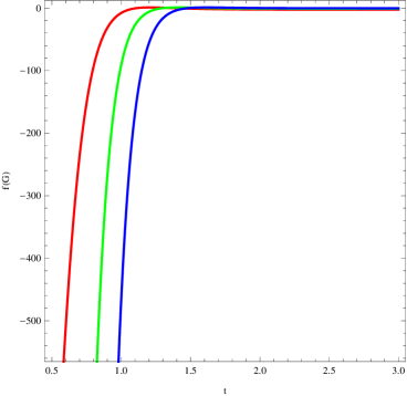
Figure 1: Plot of $f(G)$ versus $t$ for Emergent scale factor with $\beta=1.2$ (red), $\beta=1.4$ (green) and $\beta=1.6$ (blue).

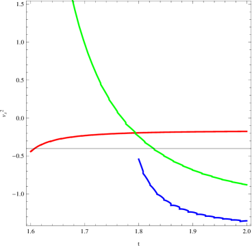
Figure 2: Plot of $v^{2}_{s}$ versus $t$ for Emergent scale factor with $\beta=1.2$ (red), $\beta=1.4$ (green) and $\beta=1.6$ (blue).

The plot of the effective EoS parameter $\omega_{eff}$ against the cosmic tine $t$ is given in Figure 3 with the help of Eq.(17). For $t=3.1$ and $\beta=1.2$, $\omega_{eff}$ crosses the phantom divide line $\omega_{eff}=-1$ from phantom to quintessence era of the expanding universe and becomes constant in the quintessence dominated universe $(-1<\omega_{eff}\leq-\frac{1}{3})$. It first expresses the matter dominated universe for $\beta=1.6$ and then it experiences decreasing behavior with the passage of time indicating the expanding universe with acceleration in quintessence era. For $\beta=1.4$, ir represents the same era of the universe. It is noted that the effective EoS parameter exhibits small oscillations for increasing $t$, however it does not affect the results corresponding to the parameter.

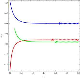
Figure 3: Plot of $\omega_{eff}$ versus $t$ for Emergent scale factor with $\beta=1.2$ (red), $\beta=1.4$ (green) and $\beta=1.6$ (blue).

IV.2 For Logamediate Scale Factor

We now consider the logamediate scale factor to discuss the evolution trajectories of the new $f(G)$ HDE model, the squared speed of sound $v_{s}^{2}$ and the effective EoS parameter $\omega_{eff}$ taking into account Eq.(17). Considering the same values of $\lambda$ and $\delta$ for the emergent case with $B=2$, we plot this scenario against cosmic time $t$ for three different values of $\beta$, i.e. $\beta=1.001,~{}1.002,~{}1.003$. For this purpose, we use Eqs.(13) and (17).

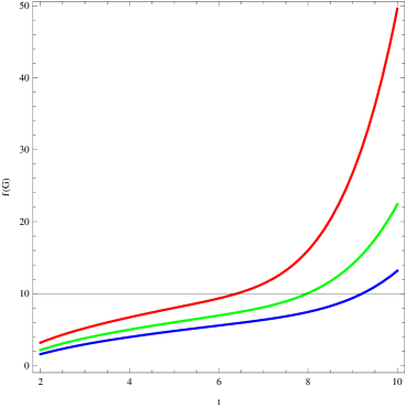
Figure 4: Plot of $f(G)$ versus $t$ for Logamediate scale factor with $\beta=1.001$ (red), $\beta=1.002$ (green) and $\beta=1.003$ (blue).

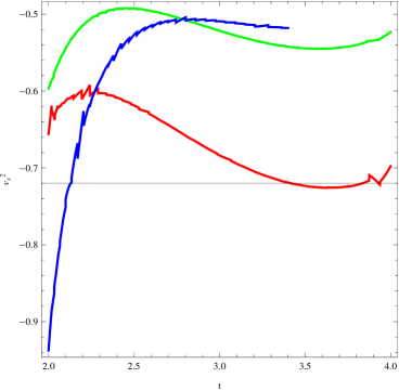
Figure 5: Plot of $v^{2}_{s}$ versus $t$ for Logamediate scale factor with $\beta=1.001$ (red), $\beta=1.002$ (green) and $\beta=1.003$ (blue).

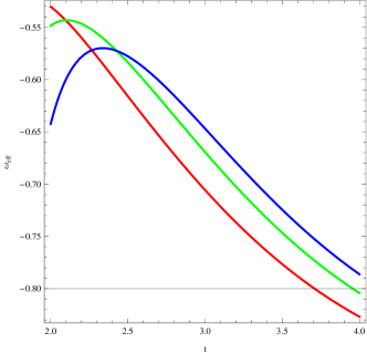
Figure 6: Plot of $\omega_{eff}$ versus $t$ for Logamediate scale factor with $\beta=1.001$ (red), $\beta=1.002$ (green) and $\beta=1.003$ (blue).

Figure 4 shows that the new $f(G)$ HDE model increases as the cosmic time $t$ increases. It carries the more steeper plot for the smaller values of $\beta$ and indicates the flatness for its higher values. Thus the model represents the increasing and positive behavior in the evolution of the universe. $v^{2}_{s}$ bears negative behavior against the cosmic time $t$ as shown in Figure 5. This implies instability of the model for all values of $\beta$ considered. Figure 6 represents the plot of $\omega_{eff}$ against the cosmic time $t$ for all the choices of $\beta$ considered here. It exhibits the quintessence region of the accelerated expansion of the universe.

IV.3 For Intermediate Scale Factor

By adopting the same procedure as for above scale factors, we discuss the same quantities for intermediate scale factor. Figures 7, 8 and 9 describe, respectively, the graphical behavior of new $f(G)$ HDE model, $v^{2}_{s}$ and $\omega_{eff}$ against the cosmic time $t$ using the scale factor considered here. We consider three different values of the parameter $\beta$, i.e. $\beta=0.04,~{}0.05,~{}0.06$ along with $B=0.5$ and same values of $\mu$ and $\lambda$ applied for the other scale factors. The graph of new $f(G)$ HDE model displays the positive and decreasing behavior with the passage of time for all values of $\beta$. In the evolving universe, this model with intermediate scale factor shows decaying behavior in the future epoch of the universe. The plot of squared speed of sound against cosmic time $t$ demonstrates the stability of the model for all values of $\beta$. However, the curve for $\beta=0.05$ may be examined as to come from instability to stable and maintain it for the future epoch while the other two curves stay always in stable region.

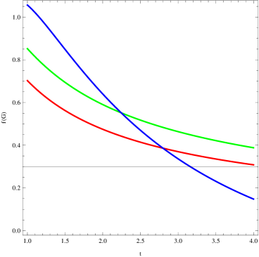
Figure 7: Plot of $f(G)$ versus $t$ for Intermediate scale factor with $\beta=0.04$ (red), $\beta=0.05$ (green) and $\beta=0.06$ (blue).

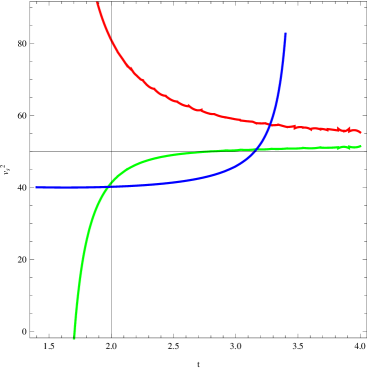
Figure 8: Plot of $v^{2}_{s}$ versus $t$ for Intermediate scale factor with $\beta=0.04$ (red), $\beta=0.05$ (green) and $\beta=0.06$ (blue).

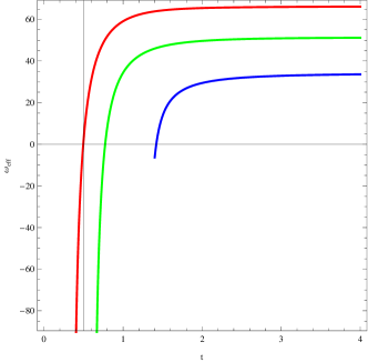
Figure 9: Plot of $\omega_{eff}$ versus $t$ for Intermediate scale factor with $\beta=0.04$ (red), $\beta=0.05$ (green) and $\beta=0.06$ (blue).

The EoS parameter bears negative behavior initially for a small value of $t$ but it increases and becomes positive. It shows the decelerating phase of the universe for the future epoch which is not compatible with the recent observations accelerating universe.

V Concluding remarks

The main aim of this work is an holographic reconstruction of $f(G)$ gravity taking as IR cut-off the recently proposed Granda-Oliveros cut-off, which is proportional to the sum of Hubble parameter and its first time derivative. We have taken here HDE with GO cut-off in order to check the more viable/workable model than already discussed reconstruction scenario. For this purpose, we have assumed three different models of the scale factor $a(t)$, i.e. the emergent, the logamediate and the intermediate one. The analytical solution of reconstructed model is a hard job, thus we have preferred to obtain numerical solutions with the help of graphs. We have constructed EoS parameter $\omega_{eff}$ as well as an analysis about stability of the model with these scale factors. The results of reconstructed scenario are as follows.

For the emergent scale factor, we have found that $f(G)$ converges to zero after a negatively increasing behavior for all values of the parameter $\beta$. Studying the squared speed of sound, it is observed that the reconstructed model is classically unstable for the future epoch for this kind of scale factor. The EoS parameter shows different behaviors according to the values of $\beta$. For $\beta=1.2$, $\omega_{eff}$ is able to cross the phantom divide line and it becomes constant in the quintessence dominated universe.

During the evolution of the universe, $f(G)$ has a positive and increasing behavior for the logamediate scale factor. The squared speed of the sound is always negative for all the values of the parameter $\beta$, implying an instability of the model for this kind of scale factor. The EoS parameter always stays in the quintessence region of the accelerated expansion of the universe for all values of the parameter $\beta$.

The graph of $f(G)$ has a positive and decreasing behavior as time passes for all values of $\beta$ incorporating the intermediate scale factor. The squared speed of the sound shows a general stability of the model for this scale factor, even if the case with $\beta=0.05$ needs particular attention since it passes from the instable to the stable region of the plot. The EoS parameter shows a decelerating phase of the universe which appears to be not compatible with recent cosmological observations.

Acknowledgment

The first author (AJ) wishes to thank the Higher Education Commission, Islamabad, Pakistan for its financial support through the Indigenous Ph.D. 5000 Fellowship Program Batch-VII. The third author (SC) wishes to acknowledge the financial support from Department of Science and Technology, Govt. of India under Project Grant no. SR/FTP/PS-167/2011.

References

- (1) Perlmutter, S. et al.: Astrophys. J. 517(1999)565.
- (2) Spergel, D.N. et al.: Astrophys. J. Suppl. 148(2003)175.
- (3) Bamba, K., Capozziello, S., Nojiri, S., Odintsov, S.D.: Astrophys Space Sci 342(2012)155.
- (4) Copeland, E.J., Sami, M., Tsujikawa, S.: Int. J. Mod. Phys. D 15(2006)1753.
- (5) Frieman, J.A., Turner, M.S., Huterer, D.: Annu. Rev. Astro. Astrophys. 46(2008)385.
- (6) Sami, M.: Curr. Sci. 97(2009)887.
- (7) Nojiri, S., Odintsov, S.D.: Phys. Lett. B 631(2005)1.
- (8) Nojiri, S., Odintsov, S.D.: Physics Reports 505(2011)59.
- (9) Olmo, G.J.: Int. J. Mod. Phys. D 20(2011)413.
- (10) Clifton, T., Ferreira, P.G., Padilla, A., Skordis, C.: Physics Reports 513(2012)1.
- (11) Nojiri, S., Odintsov, S.D.: Int. J. Geom. Meth. Mod. Phys. 4(2007)115.
- (12) Bousso, R.: Rev. Mod. Phys. 74(2002)825.
- (13) Hsu, S.D.H.: Phys. Lett. B 594(2004)13.
- (14) Huang, Q.G., Li, M.: J. Cosmol. Astropart. Phys. 8(2004)13.
- (15) Jamil, M. et al.: Int. J. Theor. Phys. (2011) 579.
- (16) Li, M.: Phys. Lett. B 603(2004)1.
- (17) Mukherjee, S., Paul, B.C., Dadhich, N.K., Maharaj, S.D., Beesham, A.: Class. Quantum Grav. 23(2006)6927.
- (18) Barrow, J.D., Liddle, A.R.: Phys. Rev. D 47(1993)5219.
- (19) Barrow, J.D., Nunes, N.J.: Phys. Rev. D 76(2007)043501.
- (20) Clarkson, C., Zunckel, C.,: Phys. Rev. Lett. 104(2010)211301.
- (21) Liu, X.M., Liu, W.B.: Astrophys. Space Sci. 334(2011)203.
- (22) Sahni, V., Starobinsky, A.: Int. J. Mod. Phys. D 15(2006)2105.
- (23) Seikel, M., Clarkson, C., Smith, M.: JCAP 06(2012)036.
- (24) Setare, M.R., Saridakis, E.N.: Phys. Lett. B 670(2008)1.
- (25) Setare, M.R., Saridakis, E.N.: Phys. Lett. B 668(2008)177.
- (26) Chattopadhyay, S., Pasqua, A.: Astrophys. Space Sci. 344(2013)269.
- (27) Jawad, A., Pasqua, A., Chattopadhyay, S.: Astrophys. Space Sci. 344(2013)489.
- (28) Rastkar, A.R., Setare, M.R., Darabi, F.: Astrophys. Space Sci. 337(2012)487.
- (29) Setare, M.R.: Int. J. Mod. Phys. D 12(2008)2219.
- (30) Paul, B.C., Ghose, S.: Gen. Relativ. Gravit.: 42(2010)795.
- (31) Khatua, P.B., Debnath, U.: Astrophys. Space Sci. 326(2010)53.
- (32) Nojiri, S., Odintsov, S.D.: J. Phys. Conf. Ser. 66(2007)012005.