Properties of Short-wavelength Oblique Alfvén and Slow Waves

Abstract

Linear properties of kinetic Alfvén waves (KAWs) and kinetic slow waves (KSWs) are studied in the framework of two-fluid magnetohydrodynamics. We obtain the wave dispersion relations that are valid in a wide range of the wave frequency $\omega$ and plasma-to-magnetic pressure ratio $\beta$. The KAW frequency can reach and exceed the ion cyclotron frequency at ion kinetic scales, whereas the KSW frequency remains sub-cyclotron. At $\beta\sim 1$, the plasma and magnetic pressure perturbations of both modes are in anti-phase, so that there is nearly no total pressure perturbations. However, these modes exhibit also several opposite properties. At high $\beta$, the electric polarization ratios of KAWs and KSWs are opposite at the ion gyroradius scale, where KAWs are polarized in sense of electron gyration (right-hand polarized) and KSWs are left-hand polarized. The magnetic helicity $\sigma\sim 1$ for KAWs and $\sigma\sim-1$ for KSWs, and the ion Alfvén ratio $R_{Ai}\ll 1$ for KAWs and $R_{Ai}\gg 1$ for KSWs. We also found transition wavenumbers where KAWs change their polarization from left- to right-hand. These new properties can be used to discriminate KAWs and KSWs when interpreting kinetic-scale electromagnetic fluctuations observed in various solar-terrestrial plasmas. This concerns, in particular, identification of modes responsible for kinetic-scale pressure-balanced fluctuations and turbulence in the solar wind.

1. Introduction

Kinetic Alfvén waves (KAWs) have been receiving recently much attention in connection to understanding turbulence at kinetic scales in the solar wind and the near-Earth space environment Chaston et al. (2008); Podesta (2013). KAWs can be generated by the MHD Alfvénic turbulence through an anisotropic cascade Howes et al. (2008); Bian et al. (2010); Zhao et al. (2013), or through non-local coupling of the MHD Alfvén waves Zhao et al. (2011, 2014). These processes provide a pathway for the turbulence to dissipate via KAWs’ damping Schekochihin et al. (2009). KAWs have been found in many in situ spacecraft measurements Chaston et al. (2008, 2009); Huang et al. (2012); Podesta (2013). Identification of KAWs is usually accomplished by analyzing characteristic wave parameters, such as the ratio of electric to magnetic perturbations Chaston et al. (2008, 2009), magnetic compressibility Podesta & TenBarge (2012), magnetic helicity Howes et al. (2010); Podesta et al. (2011); He et al. (2012), or the profile of wave dispersion Sahraoui et al. (2009, 2010); Roberts et al. (2013).

On the other hand, kinetic slow waves (KSWs) have been found indirectly by analyzing the compressible turbulent fluctuations in the solar wind turbulence Howes et al. (2012); Klein et al. (2012). KSWs have been used in the interpretation of recent observations of small-scale pressure balanced structures (PBSs) in the solar wind Yao et al. (2011, 2013), which exhibit an anti-correlation between the plasma and the magnetic pressure fluctuations. Since such small-scale PBSs can also be associated with KAWs, it is of great interest to investigate in more detail properties of the KAW and KSW modes at parallel and perpendicular kinetic scales, especially their differences.

Hollweg (1999) derived a two-fluid dispersion equation for KAWs and KSWs, and investigated properties of low-frequency KAWs, $\omega\ll\omega_{ci}$, where $\omega_{ci}$ is the ion cyclotron frequency. Another often made restricting assumption (see e.g. Shukla & Stenflo, 2000, and many others) was that the plasma beta $\beta\ll 1$ ($\beta$ is the plasma/magnetic pressure ratio). These restrictions make problematic the applicability of obtained result to the solar wind, where $\beta$ is often $\sim 1$ and the wave frequency $\omega$ that can approach and exceed $\omega_{ci}$ Huang et al. (2012); Sahraoui et al. (2012). For the quasi-perpendicular Alfvén waves with frequencies reaching and extending above $\omega/\omega_{ci}=1$, we will still use the same term KAW. The reason is that the wave dispersion and wave properties do not change much when the wave frequency crosses $\omega_{ci}$.

In the present study we relax two above restrictions and study KAWs and KSWs in a wide range of wave and plasma parameters. A two-fluid plasma model is used to simplify derivations of the wave dispersion and wave properties. The two-fluid plasma model has been proved to provide a good description for non-dissipative KAWs Hollweg (1999); Bellan (2013). We suggest that the kinetic-scale PBSs observed in the solar wind can be interpreted not only in terms of KSWs, but also in terms of KAWs, and hence both these modes can contribute to PBSs. A more detailed analysis using new mode properties we obtained in this paper is needed to reveal the dominant mode in every particular event.

In Section 2, we derive the dispersion relation of the waves for the two-fluid model. Sections 3 and 4 discuss the properties of KAWs and KSWs, respectively. A discussion and conclusion is given in Section 5. The detailed derivation of the general dispersion equation is presented in Appendix A, the wave polarization and correlation properties are given in Appendix B, and Appendix C gives the analytic expressions of the linear wave dispersion relations and the linear responses in the low-$\beta$ plasmas.

2. Dispersion relation and linear response

We shall start with the linear two-fluid equations

$$m_{\alpha}n_{0}\partial_{t}\mathbf{\delta v}_{\alpha} = n_{0}q_{\alpha}\left(\mathbf{\delta E}+\mathbf{\delta v}_{\alpha}\times\mathbf{B}_{0}\right)-\nabla P_{\alpha},$$ (1)

$$\partial_{t}\delta n_{\alpha} = -\nabla\cdot\left(n_{0}\mathbf{\delta v}_{\alpha}\right),$$ (2)

$$\nabla\times\delta\mathbf{B} = \mu_{0}\delta\mathbf{J}+\frac{1}{c^{2}}\partial_{t}\mathbf{\delta E},$$ (3)

$$\nabla\times\delta\mathbf{E} = -\partial_{t}\delta\mathbf{B},$$ (4)

where the subscript $\alpha=i,e$ represents ions and electrons, respectively, $m_{\alpha}$ is the mass, $q_{\alpha}$ is the charge, $P_{\alpha}=T_{\alpha}n_{\alpha}$ is the thermal plasma pressure, $T_{\alpha}$ is the temperature, $\mathbf{\delta v}_{\alpha}$ is the perturbed velocity, $\mathbf{B}_{0}=B_{0}\hat{\mathbf{e}}_{z}$ is the uniform external magnetic field, $\delta\mathbf{J}$ is the perturbed current density, $\delta\mathbf{E}$ and $\delta\mathbf{B}$ are the electric and magnetic field perturbations, respectively, $n_{\alpha}=n_{0}+\delta n_{\alpha}$, $n_{0}$ and $\delta n_{\alpha}$ are the background and perturbed number densities, respectively. We also assume $\omega_{pi}/\omega_{ci}\gg 1$, so that the displacement current in the Ampere’s law (3) can be neglected.

We consider all perturbed variables $\delta f$ in the form of plane waves, $\delta f\propto\delta f_{k}\mathbf{exp}(-i\omega t+i\mathbf{k}\cdot\mathbf{r})$, where $\omega$ is wave frequency and $\mathbf{k}$ is the wave vector. The waves are further assumed to propagate in the $(x,z)$ plane, that is, $\mathbf{k}=k_{\perp}\hat{\mathbf{e}}_{x}+k_{z}\hat{\mathbf{e}}_{z}$. The derivation of the general dispersion equation (A17) is given in Appendix A. Using corresponding approximations, the dispersion equation (A17) can be reduced to previously derived equations Shukla & Stenflo (2000); Zhao et al. (2010); Chen & Wu (2011). Note that the two-fluid MHD plasma theory has several limitations as compared to the kinetic plasma theory. Most importantly, the two-fluid MHD cannot describe kinetic wave-particle interactions, like Landau damping, transit-time damping, and cyclotron damping. Also, some wave modes, like ion Bernstein mode, can only be found in the kinetic theory. As a result, the highly oblique fast wave transforms into the ion Bernstein mode at $\omega>\omega_{ci}$ in the kinetic theory, whereas in the fluid theory it continuously extends from $\omega<\omega_{ci}$ to the electron cyclotron frequency $\omega\rightarrow\omega_{ce}$ (Sahraoui et al. 2012). As far as the highly oblique KAWs are concerned, the wave properties given by the two-fluid MHD are consistent nearly with those given by the kinetic theory (Sahraoui et al. 2012; Hunana et al. 2013). In particular, the KAW dispersion relation is nearly the same in two theories in the low-beta plasmas (Hunana et al. 2013). The frequency of the quasi-perpendicular slow mode also rises slowly as compared to the fast mode. Therefore, we focus on the quasi-perpendicular Alfvén and slow modes, but not the fast mode.

For quasi-perpendicular propagation, $k_{\perp}\gg k_{z}$, the cubic dispersion equation in $\omega^{2}$ (Equation (A17)) can be reduced to the quadratic equation for $\omega^{2}\ll k^{2}$$\left(V_{T}^{2}+V_{A}^{2}\right)$:

$$\omega^{4}\left[1+\lambda_{e}^{2}k_{\perp}^{2}+\lambda_{i}^{2}k_{z}^{2}+\left(1+\lambda_{e}^{2}k_{\perp}^{2}\right)^{2}\beta\right]$$

$$-\omega^{2}\left(1+2\beta+\rho^{2}k_{\perp}^{2}\right)V_{A}^{2}k_{z}^{2}+\beta V_{A}^{4}k_{z}^{4}=0,$$ (5)

which describes the dispersion relation of the Alfvén and slow waves, $\omega^{2}\sim V_{A}^{2}k_{z}^{2}$ and $\omega^{2}\sim V_{T}^{2}k_{z}^{2}$. Here $\beta=V_{T}^{2}/V_{A}^{2}$. The terms of the order $Q=m_{e}/m_{i}$ or smaller are neglected in Eq. (5). The straightforward solutions to this equation are

$$\omega^{2} = \frac{V_{A}^{2}k_{z}^{2}(1+2\beta+\rho^{2}k_{\perp}^{2})}{2\left(1+\lambda_{e}^{2}k_{\perp}^{2}+\lambda_{i}^{2}k_{z}^{2}+\left(1+\lambda_{e}^{2}k_{\perp}^{2}\right)^{2}\beta\right]}\times$$ (6)

$$\left[1\pm\sqrt{1-4\beta\frac{1+\lambda_{e}^{2}k_{\perp}^{2}+\lambda_{i}^{2}k_{z}^{2}+\left(1+\lambda_{e}^{2}k_{\perp}^{2}\right)^{2}\beta}{\left(1+2\beta+\rho^{2}k_{\perp}^{2}\right)^{2}}}\right],$$

where “+” stands for KAWs and “-” for KSWs. Dispersion relation derived by Hollweg (1999) is recovered from (6) in the low-frequency limit $\lambda_{i}^{2}k_{z}^{2}\ll 1$ (hence $\omega^{2}\ll\omega_{ci}^{2}$), and $\left(1+\lambda_{e}^{2}k_{\perp}^{2}\right)\left(1+\beta\right)\simeq 1+\beta+\lambda_{e}^{2}k_{\perp}^{2}$.

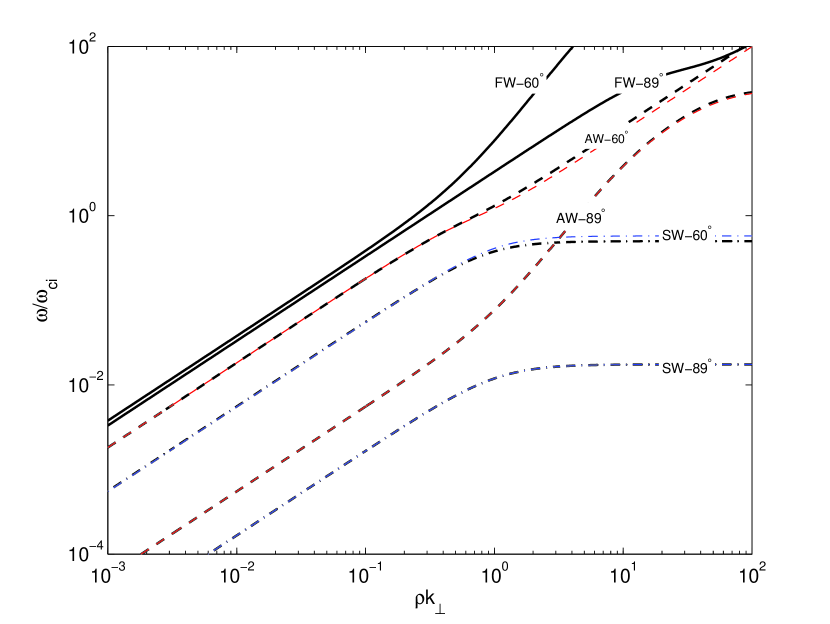
Figure 1.— Comparison of the dispersion relations (6) (thin dashed lines are for Alfvén waves; thin dot-dashed lines are for slow waves) with the wave modes obtained from the general dispersion equation (A17) (thick solid lines are for fast waves; thick dashed lines are for Alfvén waves; thick dot-dashed lines are for slow waves). The two propagation angles are $\theta=60^{\circ}$ and $89^{\circ}$, and $\beta=0.1$.

Figure 1 compares numerical solutions of the general dispersion equation (A17) and the dispersion relations (6) obtained for the quasi-perpendicular wave propagation. At such oblique propagation, the fast mode has significantly higher frequencies than the other two modes. The remaining KAW and KSW modes behave differently. Similarly to the fast mode, the KAW mode frequency increases monotonously with increasing wavenumber and exceeds the $\omega_{ci}$ at some wavelength close to the ion gyroradius. On the contrary, the KSW frequency slows down it increase above the ion gyroradius scale and never cross $\omega=\omega_{ci}$. From this figure one can see that the quasi-perpendicular dispersion relations (6) are also valid down to $\theta\sim 60^{\circ}$.

The physical quantities associated with the KAW and KSW dispersion relations can be easily obtained from Equations (A1)–(A6) and (A11)–(A15):

$$\delta\mathbf{B} = -i\frac{\omega_{ci}}{\omega}\Upsilon_{1}\delta B_{y}\hat{\mathbf{e}}_{x}+\delta B_{y}\hat{\mathbf{e}}_{y}+i\frac{k_{\perp}}{k_{z}}\frac{\omega_{ci}}{\omega}\Upsilon_{1}\delta B_{y}\hat{\mathbf{e}}_{z},$$ (7)

$$\delta\mathbf{E} = \frac{\omega}{k_{z}}\left(1+\lambda_{e}^{2}k^{2}+\Upsilon_{2}\frac{\widetilde{T}_{e}}{\widetilde{T}_{i}}\right)\widetilde{T}_{i}\delta B_{y}\hat{\mathbf{e}}_{x}+i\frac{\omega_{ci}}{k_{z}}\Upsilon_{1}\delta B_{y}\hat{\mathbf{e}}_{y}$$ (8)

$$+\frac{\omega}{k_{\perp}}\left(1+\lambda_{e}^{2}k^{2}+\Upsilon_{2}\frac{\widetilde{T}_{e}}{\widetilde{T}_{i}}-\frac{1}{\widetilde{T}_{i}}\right)\widetilde{T}_{i}\delta B_{y}\hat{\mathbf{e}}_{z},$$

$$\delta\mathbf{v}_{i} = i\frac{\omega_{ci}}{k_{z}}\left(\Upsilon_{2}-\frac{V_{A}^{2}k_{z}^{2}}{\omega^{2}}\right)\frac{\delta B_{y}}{B_{0}}\hat{\mathbf{e}}_{x}-\frac{V_{A}^{2}k_{z}}{\omega}\frac{\delta B_{y}}{B_{0}}\hat{\mathbf{e}}_{y}$$ (9)

$$+i\frac{\omega_{ci}}{k_{\perp}}\left(\Upsilon_{2}-1\right)\frac{\delta B_{y}}{B_{0}}\hat{\mathbf{e}}_{z},$$

$$\delta\mathbf{v}_{e} = i\frac{\omega_{ci}}{k_{z}}\left(\Upsilon_{2}-\frac{V_{A}^{2}k_{z}^{2}}{\omega^{2}}+\lambda_{i}^{2}k_{z}^{2}\right)\frac{\delta B_{y}}{B_{0}}\hat{\mathbf{e}}_{x}$$ (10)

$$-\frac{\omega}{k_{z}}\left(1+\lambda_{e}^{2}k^{2}-Q\frac{V_{A}^{2}k_{z}^{2}}{\omega^{2}}\right)\frac{\delta B_{y}}{B_{0}}\hat{\mathbf{e}}_{y}$$

$$+i\frac{\omega_{ci}}{k_{\perp}}\left(\Upsilon_{2}-\lambda_{i}^{2}k_{\perp}^{2}-1\right)\frac{\delta B_{y}}{B_{0}}\hat{\mathbf{e}}_{z},$$

where

$$\Upsilon_{1} = \left(1+\lambda_{e}^{2}k^{2}\right)\frac{\omega^{2}}{V_{A}^{2}k^{2}}-\frac{k_{z}^{2}}{k^{2}},$$

$$\Upsilon_{2} = \left(1+\lambda_{e}^{2}k^{2}\right)^{2}\frac{\omega^{2}}{V_{A}^{2}k^{2}}-\frac{k_{z}^{2}}{k^{2}}+\frac{V_{A}^{2}k_{z}^{2}}{\omega^{2}}-\lambda_{i}^{2}k_{z}^{2},$$

The number density and the parallel magnetic field are related by

$$\frac{\delta n}{n_{0}}=-\frac{1}{\beta}\frac{k^{2}}{k_{\perp}^{2}}\frac{1+\lambda_{e}^{2}k^{2}-\Upsilon_{2}}{1+\lambda_{e}^{2}k^{2}-V_{A}^{2}k_{z}^{2}/{\omega^{2}}}\frac{\delta B_{z}}{B_{0}}.$$ (11)

These relations (7)–(11) can be used in the diagnostics of experimentally observed wave phenomena.

3. KAW properties

KAWs behave differently in different $\beta$ regimes, namely, the inertial regime $\beta<m_{e}/m_{i}$, the kinetic regime $m_{e}/m_{i}<\beta<1$, and the high-$\beta$ regime $\beta\gtrsim 1$. Thus, we will investigate the KAW properties for the representative values $\beta=10^{-4}$, typical in the Earth’s ionosphere and the solar flare loops, $\beta=10^{-2}$, typical in the Earth’s magnetosphere and the solar corona, and $\beta=1$, typical in the solar wind at $\sim 1$AU.

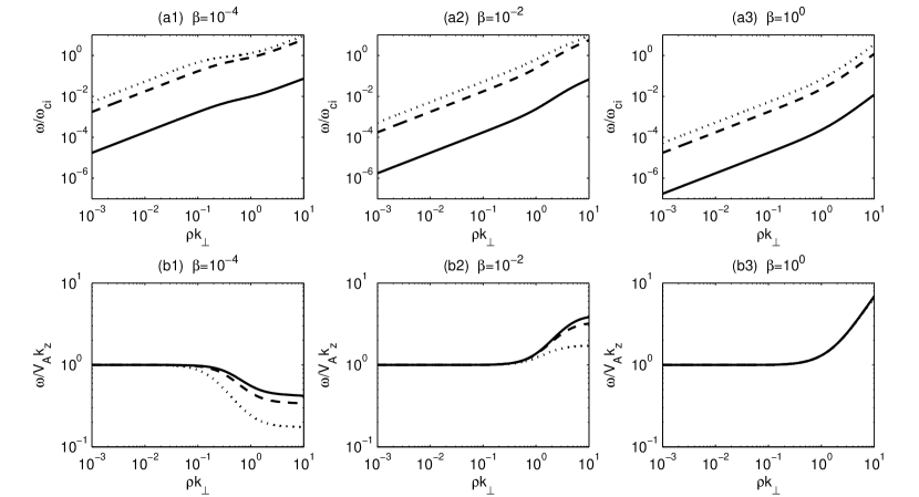
Figure 2.— Wave frequency of KAWs in three different $\beta$ regimes: inertial regime $\beta=10^{-4}$, kinetic regime $\beta=10^{-2}$, and high-$\beta$ regime $\beta=1$. The dotted, dashed, and solid lines represent the propagating angle $\theta=87^{\circ},89^{\circ}$, and $89^{\circ}.99$, respectively. (a) $\omega$ is normalized by $\omega_{ci}$; (b) $\omega$ normalized by $V_{A}k_{z}$. The equal electron and ion temperatures, $T_{e}=T_{i}$, is used here and following figures.

From Figure 2 one can see that the KAW frequency is larger than the ion-cyclotron frequency, $\omega\gtrsim\omega_{ci}$, when $k_{\perp}\rho=1$ and $\theta=87^{\circ}$ or $89^{\circ}$, but $\omega/\omega_{ci}<1$ for extremely oblique propagation, $\theta=89^{\circ}.99$. This is consistent with the result in Sahraoui et al. (2012) that $\omega/\omega_{ci}<1$ at all scales as the propagating angle $\theta>\theta_{\mathrm{crit}}=\mathrm{cos}^{-1}(Q)\simeq 89^{\circ}.97$.

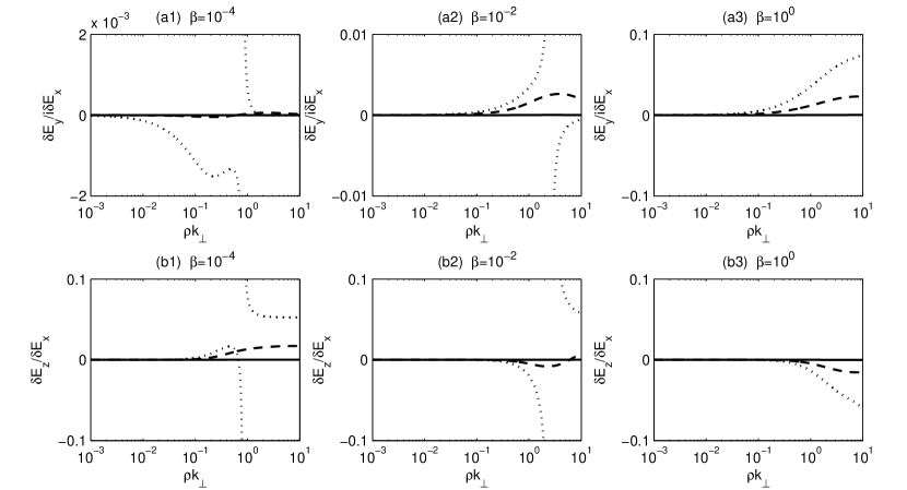
Figure 3.— Electric polarization ratios $\delta E_{y}/(i\delta E_{x})$ and $\delta E_{z}/\delta E_{x}$ for KAWs. The dotted, dashed, and solid lines represent the propagating angles $\theta=87^{\circ},$ $89^{\circ}$, and $89^{\circ}.99$, respectively.

Figure 3 presents the electric polarization of KAWs. The waves are polarized elliptically (almost linearly in low-$\beta$ plasmas), $P_{\delta E,\mathbf{B}_{0}}=\delta E_{y}/\left(i\delta E_{x}\right)<1$. At relatively small $\rho k_{\perp}$, the polarization parameter is positive, $P_{\delta E,\mathbf{B}_{0}}>0$, in the kinetic and high-$\beta$ regimes, which corresponds to the right-hand polarization, as was first shown by Gary (1986); Hollweg (1999). However, at larger $\rho k_{\perp}>1$ there are several transition points where $\delta E_{x}$ passes through zero and $\delta E_{y}/i\delta E_{x}$ and $\delta E_{z}/\delta E_{x}$ change their signs. These polarization reversals are discussed in more detail below.

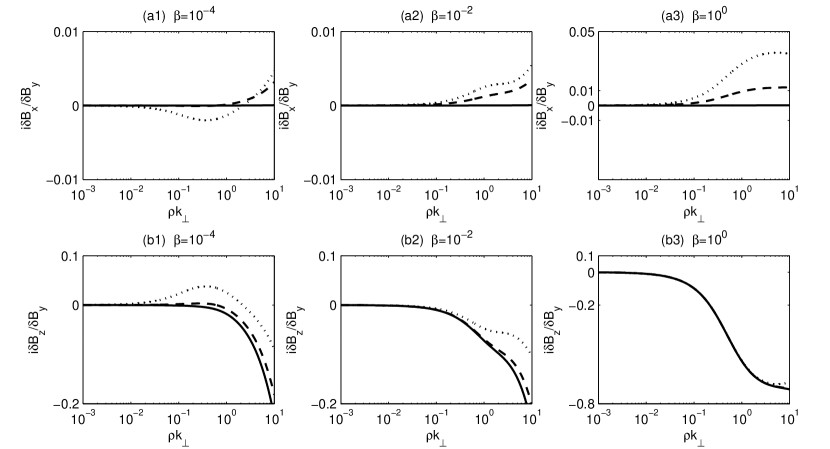
Figure 4.— Magnetic polarization ratios $i\delta B_{x}/\delta B_{y}$ and $i\delta B_{z}/\delta B_{y}$ for KAWs. The dotted, dashed, and solid lines represent the wave propagation angles $\theta=87^{\circ},$ $89^{\circ}$, and $89^{\circ}.99$, respectively.

Figures 4 and 5 show the magnetic polarization and the magnetic helicity $\sigma$ of KAWs. At the ion scale $\rho k_{\perp}\sim 1$ we observe quite small $i\delta B_{x}/\delta B_{y}\sim 0.01$, but the values of $i\delta B_{z}/\delta B_{y}$ are larger. For $\rho k_{\perp}\lesssim 1$ the KAW helicity is right-hand $(\sigma<0)$ in the inertial regime but becomes left-hand at larger $\beta$ (it also becomes left-hand in the inertial range at larger $\rho k_{\perp}$). 

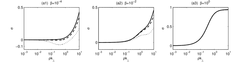
Figure 5.— Magnetic helicity $\sigma$ of KAWs. The dotted, dashed, and solid lines represent the propagation angles $\theta=87^{\circ},$ $89^{\circ}$, and $89^{\circ}.99$, respectively.

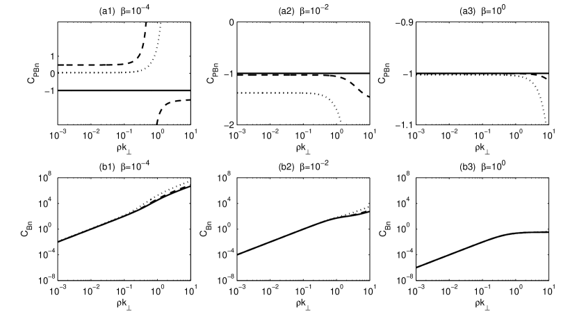
Figure 6.— Pressure correlation $C_{PBn}$ and compressibility $C_{Bn}$ of KAWs. The dotted, dashed, and solid lines represent the propagation angles $\theta=87^{\circ},$ $89^{\circ}$, and $89^{\circ}.99$, respectively.

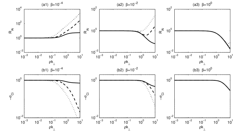
Figure 7.— Ion Alfvén ratio $R_{Ai}$ and cross helicity $\sigma_{Ci}$ of KAWs. The dotted, dashed, and solid lines represent the propagation angles $\theta=87^{\circ},89^{\circ}$, $89^{\circ}$, and $89^{\circ}.99$, respectively.

Figure 6 presents the plasma-magnetic pressure correlation $C_{PBn}=\frac{\gamma\left(T_{i}+T_{e}\right)\delta n}{\delta B_{z}B_{0}/\mu_{0}}$ and compressibility $C_{Bn}=\frac{\delta n^{2}/n_{0}^{2}}{\delta B^{2}/B_{0}^{2}}$ of KAWs. It is interesting to observe the pressure balance $C_{PBn}\simeq-1$ in the extremely oblique KAWs $(\theta=89^{\circ}.99)$ at arbitrary $\beta$. $C_{PBn}\simeq-1$ also holds for the arbitrary propagation angle in the high-$\beta$ plasmas. Note several transition points in the inertial regime where $C_{Bn}$ changes its sign, which occur when $k_{z}^{2}/k_{\perp}^{2}-\left(1+\lambda_{e}^{2}k_{\perp}^{2}\right)\beta=0$. $C_{Bn}$ nearly follows the approximate expression $C_{Bn}\simeq\rho^{2}k_{\perp}^{2}\left(1+\lambda_{e}^{2}k_{\perp}^{2}+\lambda_{i}^{2}k_{z}^{2}\right)/\beta\left({1+\rho^{2}k_{\perp}^{2}}\right)$ that is valid for the low $\beta$.

Figure 7 presents the ion Alfvén ratio $R_{Ai}$ and the ion cross helicity $\sigma_{Ci}$ of KAWs. $R_{Ai}$ and $\sigma_{Ci}$ can be rewritten as $R_{Ai}=\delta v_{i}^{2}/\delta v_{B}^{2}$ and $\sigma_{Ci}=2\left(\delta\mathbf{v}_{i}\cdot\delta\mathbf{v}_{B}^{\ast}\right)/\left(\delta v_{i}^{2}+\delta v_{B}^{2}\right)$, where $\delta v_{B}$ is the magnetic perturbation in the units of Alfvén speed. The ion cross-helicity becomes nearly zero, $\sigma_{Ci}\sim 0$, as the strong velocity mismatch appears, $\delta v_{i}\gg\delta v_{B}$ (for the kinetic scale $\lambda_{e}k_{\perp}>1$ waves with $\rho k_{\perp}>10^{-2}$ in the inertial regime) or $\delta v_{B}\gg\delta v_{i}$ (for KAWs with $\rho k_{\perp}>1$ in the high-$\beta$ plasmas).

In the following sub-sections we consider the electric field polarization and its reversal in more detail.

3.1. Electric Polarization and Its Reversal

In the limit $k_{\perp}\gg k_{z}$, from the expression (8) we get the polarization ratio

$$\frac{\delta E_{y}}{\delta E_{x}}=i\frac{\omega}{\omega_{ci}}\frac{1}{\lambda_{i}^{2}k_{\perp}^{2}}\frac{\left(1+\lambda_{e}^{2}k_{\perp}^{2}\right)\frac{\omega^{2}}{V_{A}^{2}k_{z}^{2}}-1}{\widetilde{T}_{i}\left(1+\lambda_{e}^{2}k_{\perp}^{2}\right)\frac{\omega^{2}}{V_{A}^{2}k_{z}^{2}}+\widetilde{T}_{e}\left(1-\frac{\omega^{2}}{\omega_{ci}^{2}}\right)}.$$ (12)

The sense of the wave polarization can change when the numerator or denominator of this expression passes through zero, which correspond to $\delta E_{y}=0$ or $\delta E_{x}=0$ , respectively. The $\delta E_{x}=0$ transition occurs at

$$\left(\frac{\omega^{2}}{\omega_{ci}^{2}}-1\right)=\frac{\widetilde{T}_{i}}{\widetilde{T}_{e}}\left(1+\lambda_{e}^{2}k_{\perp}^{2}\right)\frac{\omega^{2}}{V_{A}^{2}k_{z}^{2}}>0,$$ (13)

which implies high-frequency $\omega>\omega_{ci}$ waves at the transition point. For the low-frequency waves ($\omega\ll\omega_{ci}$), there are no such transition points. In low-$\beta$ limit this transition can occur as

$$\lambda_{i}^{2}k_{z}^{2}=\frac{\left(1+\lambda_{e}^{2}k_{\perp}^{2}\right)\left(1+\left(1+\rho^{2}k_{\perp}^{2}\right)\widetilde{T}_{i}/\widetilde{T}_{e}\right)}{\rho^{2}k_{\perp}^{2}}.$$ (14)

The $\delta E_{y}=0$ transition occurs at

$$\frac{\omega^{2}}{V_{A}^{2}k_{z}^{2}}=\frac{1}{1+\lambda_{e}^{2}k_{\perp}^{2}}<1.$$ (15)

This transition implies sub-Alfvénic phase velocities of KAWs and is possible only due to finite $\lambda_{i}^{2}k_{z}^{2}$. In low-$\beta$ limit (15) gives the transition wavenumber

$$\rho^{2}k_{\perp\mathrm{tr}}^{2}=\frac{m_{i}}{m_{e}}\left(\frac{1}{\tan^{2}\theta}-\beta\right).$$ (16)

With growing $\rho^{2}k_{\perp}^{2}$, the transition occurs from the left- to right-hand polarization. For this transition to occur, the wave propagation angle should be less than certain value,

$$\theta<\theta_{\mathrm{cr}}=\arctan\frac{1}{\sqrt{\beta}}.$$ (17)

Otherwise, the wave is always right-hand polarization. Only in this last case the conclusion by Gary (1986); Hollweg (1999) holds that KAWs are right-hand polarized.

The above analysis indicates that KAWs can be both left- and right-hand polarized.

3.2. The Low-$\beta$ Low-frequency Limit

For KAWs in low-$\beta$ plasmas, $\beta\ll 1$, we get

$$\frac{\delta E_{y}}{\delta E_{x}}=i\beta\frac{\omega}{\omega_{ci}}\frac{1}{1+\rho_{i}^{2}k_{\perp}^{2}}\frac{\left(1+\lambda_{e}^{2}k_{\perp}^{2}\right)-\lambda_{i}^{2}k_{z}^{2}/\rho^{2}k_{\perp}^{2}}{\left(1+\lambda_{e}^{2}k_{\perp}^{2}\right)-\lambda_{i}^{2}k_{z}^{2}\rho_{s}^{2}k_{\perp}^{2}/\left(1+\rho_{i}^{2}k_{\perp}^{2}\right)}.$$ (18)

At small $\lambda_{i}^{2}k_{z}^{2}\ll 1$ (i.e. in the low-frequency range) the denominator of the above expression is dominated by the term $\left(1+\lambda_{e}^{2}k_{\perp}^{2}\right)$, and we arrive to

$$\frac{\delta E_{y}}{\delta E_{x}}=i\beta\frac{\omega}{\omega_{ci}}\frac{1}{1+\rho_{i}^{2}k_{\perp}^{2}}\left(1-\frac{1}{\left(\beta+\frac{m_{e}}{m_{i}}\rho^{2}k_{\perp}^{2}\right)\tan^{2}\theta}\right),$$ (19)

which indicates that the electric polarization depends on the magnitude of $k_{\perp}$ compared to the ion kinetic scales. In the limit $\beta\tan^{2}\theta\gg 1$, our expression (19) simplifies to

$$\frac{\delta E_{y}}{\delta E_{x}}=i\beta\frac{\omega}{\omega_{ci}}\frac{1}{1+\rho_{i}^{2}k_{\perp}^{2}}.$$ (20)

In this limit the waves are always right-hand polarized. In principle, this conclusion agrees with previous results Gary (1986); Hollweg (1999). In the long-wavelength limit $\rho_{i}^{2}k_{\perp}^{2}\ll 1$, Equation (19) reduces to the approximate analytical formula Equation (46) by Hollweg (1999),

$$\frac{\delta E_{x}}{\delta E_{y}}=i\beta\frac{\omega}{\omega_{ci}}.$$ (21)

4. KSW properties

Before discussing properties of the oblique slow waves in the two-fluid MHD, it is instructive to mention some their known properties in the kinetic theory. At general oblique propagation, the slow/sound wave extends to the frequency larger than the ion cyclotron frequency as showed in Figure 1 by Krauss-Varban et al. (1994) for the propagation angle $\theta=30^{\circ}$. At larger propagation angles, large wavenumbers are required for the waves to reach the ion-cyclotron frequency, and for quasi-perpendicular propagation slow waves remain sub-cyclotron in the wide range of perpendicular wavenumber, up to large values of $\rho^{2}k_{\perp}^{2}$. In the two-fluid MHD, the frequency of quasi-perpendicular KSWs always remains sub-cyclotron:

$$\frac{\omega}{\omega_{ci}}=\frac{k_{z}}{k_{\perp}}\sqrt{\frac{\rho^{2}k_{\perp}^{2}}{1+\rho^{2}k_{\perp}^{2}}}<1\mathrm{\quad for\quad}\frac{k_{z}}{k_{\perp}}\leq 1.$$

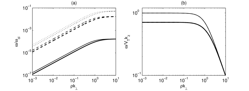
Figure 8.— Wave frequency of KSWs in three different $\beta$ regimes, the inertial regime ($\beta=10^{-4}$, the thin lines), the kinetic regime ($\beta=10^{-2}$, the middle lines), and the high-$\beta$ regime ($\beta=1$, the thick lines), where the dotted, dashed, and solid lines represent the propagating angles $\theta=87^{\circ},$ $89^{\circ}$, and $89^{\circ}.99$, respectively. The lines in the inertial regime are the same as in the kinetic regime. (a) $\omega$ is normalized by $\omega_{ci}$; (b) $\omega$ normalized by $V_{T}k_{z}$.

The KSW dispersion is showed in Figure 8 in terms of the phase velocity $\omega/\left(V_{T}k_{z}\right)$, which exhibits also a depression at high $\beta$ in the long-wavelength limit. 

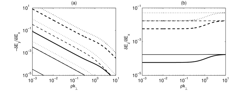
Figure 9.— Electric-field polarization $\delta E_{y}/\left(i\delta E_{x}\right)$ and $\delta E_{z}/\delta E_{x}$ of KSWs, where the lines have the same meaning as in Figure 8.

Figure 9 presents the electric polarization of KSWs. The polarization parameter $P_{E,B_{0}}=E_{y}/\left(i\delta E_{x}\right)<0$ means the left-hand KSW polarization. $\delta E_{x}$ becomes the dominant component for the waves at the ion gyroradius scale $(\rho k_{\perp}\sim 1)$. The KSW electric field polarization ratios can be approximated as $i\delta E_{y}/\delta E_{x}\simeq\beta k_{z}/\left({\rho k_{\perp}^{2}\sqrt{1+\rho^{2}k_{\perp}^{2}}}\right)$, and $\delta E_{z}/\delta E_{x}=k_{z}/k_{\perp}$.

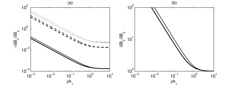
Figure 10.— Magnetic-field polarization $i\delta B_{x}/\delta B_{y}$ and $\delta B_{z}/\delta B_{y}$ of KSWs, where the lines have the same meaning as in Figure 8.

Figure 10 presents the magnetic polarization of KSWs. For the long wavelength waves ($\rho k_{\perp}\ll 1$), the compressible magnetic field perturbation $\delta B_{z}$ is the dominant component, $|\delta B_{z}/\delta B_{x,y}|\gg 1$. However, $\delta B_{y}$ becomes as important as $\delta B_{z}$ when the wavelength approaches the ion gyroradius scale, where $\delta B_{y}\simeq\delta B_{z}\gg\delta B_{x}$. The magnetic field polarization ratios nearly follow the approximate relations $i\delta B_{x}/\delta B_{y}=-\left(k_{z}/k_{\perp}\right)\sqrt{1+1/\rho^{2}k_{\perp}^{2}}$ and $i\delta B_{z}/\delta B_{y}=\sqrt{1+1/\rho^{2}k_{\perp}^{2}}$.

The helicity $\sigma$ in the low-$\beta$ plasmas can be written as $\sigma=-2\rho k_{\perp}\left(1+\rho^{2}k_{\perp}^{2}\right)^{1/2}/\left(1+2\rho^{2}k_{\perp}^{2}\right)$, which indicates that $\sigma$ decreases from $0$ to $-1$ as $\rho k_{\perp}$ increases from $10^{-3}$ to $10$. This behavior is seen from Figure 11.

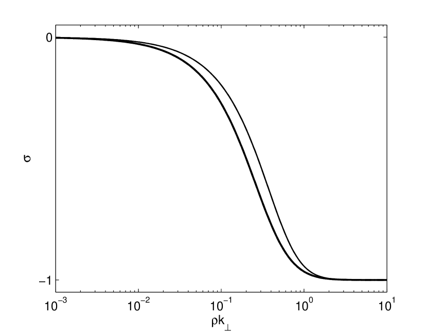
Figure 11.— Magnetic helicity of KSWs. The lines have the same meaning as in Figure 8.

Figure 12 presents the plasma/magnetic pressure correlation $C_{PBn}$ and the compressibility $C_{Bn}$ of KSWs. The behavior of these functions is in accordance with the theoretic predictions that $C_{PBn}\simeq-1$ and $C_{Bn}\simeq\left(1+\rho^{2}k_{\perp}^{2}\right)/\left(1+2\rho^{2}k_{\perp}^{2}\right)/\beta^{2}$ in the low-$\beta$ plasma. Note that $C_{PBn}$ and $C_{Bn}$ in the high-$\beta$ plasmas can be approximated by the same expressions.

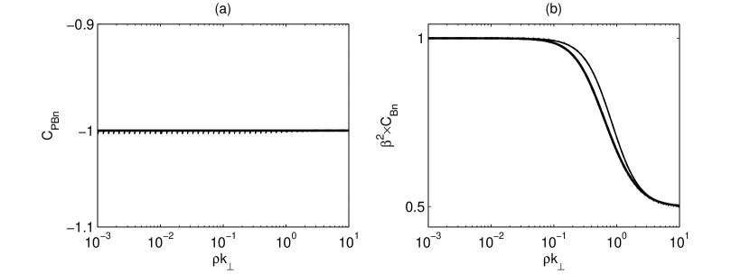
Figure 12.— Plasma/magnetic pressure ratio $C_{PBn}$ and compressibility $C_{Bn}$ of KSWs. The lines have the same meaning as in Figure 8.

Figure 13 presents the ion Alfvén ratio $R_{Ai}$ and the cross-helicity $\sigma_{Ci}$ of KSWs. $\delta v_{i}$ is nearly equal $\delta v_{B}$ in the long-wavelength waves $(\rho k_{\perp}\ll 1)$ in high-$\beta$ plasmas. In other cases $\delta v_{i}$ dominates over $\delta v_{B}$, $\delta v_{i}>\delta v_{B}$. The corresponding expressions in the low-$\beta$ plasmas are $R_{Ai}\simeq\left(1+2\rho^{2}k_{\perp}^{2}\right)/\beta$ and $\sigma_{Ci}\simeq-2\sqrt{\beta/\left(1+\rho^{2}k_{\perp}^{2}\right)}$.

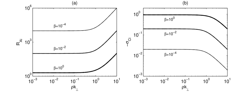
Figure 13.— Ion Alfvén ratio $R_{Ai}$ and cross-helicity $\sigma_{Ci}$ of KSWs. The lines have the same meaning as in Figure 8.

5. Discussion and conclusion

Our study shows that the Alfvén wave frequency $\omega$ at the ion gyroscale $\rho k_{\perp}\sim 1$ is smaller than the ion-cyclotron frequency $\omega_{ci}$ for extremely oblique propagation, say for $\theta=89^{\circ}.99$. In agreement with (Sahraoui et al. 2012), the KAW frequency can reach $\omega_{ci}$ for propagation angle $\theta\leq 89^{\circ}.97$. At $\rho k_{\perp}\sim 1$, $\omega$ can reach and exceed $\omega_{ci}$ for the propagation angles $\sim 87^{\circ}$ or less. At smaller propagating angles, the frequency $\omega\sim\omega_{ci}$ occurs at smaller wavenumbers. In the solar-terrestrial plasmas, the high-frequency KAWs may be generated through the Alfvénic turbulent cascade Huang et al. (2012), excited kinetically by the field-aligned currents and ion beams Voitenko & Goossens (2002, 2003), or by phase mixing combined with cyclotron sweep of Alfvén waves Voitenko & Goossens (2006) .

Our study investigated KAWs and KSWs in a wide range of $\beta,$ covering a wide range of conditions in most solar-terrestrial plasmas. Several mode properties of KAWs are totally different in the limits $\beta<m_{e}/m_{i}$ (so-called inertial range) and $\beta>m_{e}/m_{i}$ (kinetic range). So, we confirmed that the KAW phase velocity $\omega/k_{z}$ in the inertial range decreases with increasing $k_{\perp}$, but increases in the kinetic and high-$\beta$ ranges Goertz & Boswell (1979); Lysak & Lotko (1996); Stasiewicz et al. (2000)). The electric polarization ratios of KAWs are also obviously different in these two distinct $\beta$ ranges. Namely, except for the case of extremely oblique waves, at smaller $k_{\perp}$ KAWs are left-hand polarized in the inertial range and right-hand in the kinetic/high-$\beta$ ranges. The magnetic helicity at these wavenumbers is right-hand for $\beta<m_{e}/m_{i}$ and left-hand for $\beta>m_{e}/m_{i}$. At higher $k_{\perp}$ they undergo two polarization reversals defined by (13) and (15). These new polarization properties of KAWs, especially polarization reversals, are quite specific and can be used as a critical test for the mode identification in the solar wind and terrestrial magnetosphere. In addition to the Landau dissipation caused by the parallel electric field fluctuations of KAWs, the perpendicular electric-field can induce the occurrence of the cyclotron resonant damping as the frequency of KAWs reaches or exceeds the ion cyclotron frequency (Voitenko & Goossens 2002, 2003). The cyclotron-resonant damping (Kennel & Wong 1967; Marsch 2006) does not require purely left-hand or purely right-hand polarizations of Alfvén waves. When the resonant-cyclotron condition $\omega\left(k_{z}\right)-k_{z}v_{z}=n\omega_{ci}$ is satisfied for the oblique waves, there are two resonance cases depending on the interaction with $E_{x}$ or $E_{y}$ (Hollweg & Markovskii 2002), where $v_{z}$ is the parallel velocity of particles. $E_{x}$ can cause the cyclotron resonance if the particles stay in the phase with the waves, whereas the resonance relating to $E_{y}$ strongly depends on the x-position of the particles (Hollweg & Markovskii 2002). Both Landau and cyclotron dampings are crucial when investigating the turbulence dissipation channels at kinetic scales. On the contrary, the KSWs properties are nearly the same in all $\beta$ ranges and can be approximately described by the approximate expressions for the low-$\beta$ plasmas given in Section 4.

Our study provided a clear evidence of anti-correlation between the plasma and magnetic pressures for both KAWs and KSWs in high-$\beta$ plasmas. This makes the total pressure fluctuations almost zero, $\delta P_{tot}\simeq 0$, which resembles the main common property of the observed PBSs Yao et al. (2011). Kellogg & Horbury (2005) and Yao et al. (2011) used the Cluster data, which have a high time resolution of 0.2 s for the plasma number density and magnetic field, and found that the scales of PBSs extend down to the ion scale. Kellogg & Horbury (2005) interpreted these kinetic-scale PBSs in terms of KSWs. However, KAWs may be an alternative explanation since they also drive anti-correlated number density and magnetic field fluctuations. Again, one needs more mode properties to discriminate which mode dominates in PBSs, KSW or KAW. Our results reveal three different properties that distinguish these modes at the ion gyroradius scale: (1) right-hand electric polarization for KAWs and left-hand for KSWs; (2) magnetic helicity $\sigma\sim 1$ for KAWs and $\sigma\sim-1$ for KSWs; (3) Alfvén ratio $R_{Ai}\ll 1$ for KAWs and $R_{Ai}\gg 1$ for KSWs. Besides, the large-scale Alfvén waves, permeating the solar wind, can nonlinearly excite simultaneous KSWs and KAWs Zhao et al. (2014), which both can contribute to the observed PBSs. This implies that PBSs may be KSWs, or KAWs, or a mixture of KSWs and KAWs. A recent work (Hollweg et al. 2014) showed that the highly-oblique slow mode has the small variation of $P_{tot}$ in the three-fluid plasmas consisting of fully-ionized hydrogen and a heavy ion drifting along the background magnetic field. Therefore, one needs addition tests for a more careful identification of the wave modes producing the observed kinetic-scale PBSs.

In summary, we revealed several new mode properties of KAWs and KSWs accounting for the kinetic effects of the ion and electron thermal pressure and inertia. For KAWs, their frequency can reach and exceed the ion cyclotron frequency at the ion kinetic scales, where both the thermal and the inertial ion effects are important. The polarization properties of KAWs are different in different $\beta$ ranges and depend on both the propagation angle $\theta$ and the normalized perpendicular wavenumber $\rho k_{\perp}$. It appeared that KAWs undergo two reversals of electric polarization defined by the zeros of denominator (13) and the numerator (15) of (12). In particular, in low-$\beta$ plasmas less oblique KAWs (17) are left-hand polarized at longer wavelengths and right-hand at shorter wavelengths. These properties are important for the turbulence cascade transition across the ion-cyclotron frequency, where it can be partially dissipated by the ion-cyclotron resonance, in such a way that the left-hand KAWs possess stronger dissipation as compared to the right-hand ones.

For KSWs, its frequency is always smaller than ion cyclotron frequency and the mode is left-hand polarized. At the ion kinetic scales, $\rho k_{\perp}\sim 1$, the electric and magnetic KSW components obey $|\delta E_{y}|\ll|\delta E_{x}|$, $|\delta B_{x}|\ll|\delta B_{y}|$, and $|\delta B_{z}|\simeq|\delta B_{y}|$. All these properties of KSWs can be described approximately by the reduced expression obtained in the low-$\beta$ limit.

These new properties are important for understanding short-wavelength Alfvén and slow modes and can be used in interpreting waves and turbulence at kinetic scales.

Appendix A The general dispersion equation

From the momentum Equation (1), the ion and electron velocities are found as

$$\Lambda_{i}\delta v_{ix} = -i\frac{\omega}{B_{0}\omega_{ci}}\delta E_{x}+\frac{1}{B_{0}}\delta E_{y}-\frac{\gamma T_{i}\omega k_{\perp}}{m_{i}\omega_{ci}^{2}}\frac{\delta n}{n_{0}},$$ (A1)

$$\Lambda_{i}\delta v_{iy} = -\frac{1}{B_{0}}\delta E_{x}-i\frac{\omega}{B_{0}\omega_{ci}}\delta E_{y}+i\frac{\gamma T_{i}k_{\perp}}{m_{i}\omega_{ci}}\frac{\delta n}{n_{0}},$$ (A2)

$$\delta v_{iz} = i\frac{e}{m_{i}\omega}\delta E_{z}+\frac{\gamma T_{i}k_{z}}{m_{i}\omega}\frac{\delta n}{n_{0}},$$ (A3)

$$\Lambda_{e}\delta v_{ex} = i\frac{Q\omega}{B_{0}\omega_{ci}}\delta E_{x}+\frac{1}{B_{0}}\delta E_{y}-\frac{Q\gamma T_{e}\omega k_{\perp}}{m_{i}\omega_{ci}^{2}}\frac{\delta n}{n_{0}},$$ (A4)

$$\Lambda_{e}\delta v_{ey} = -\frac{1}{B_{0}}\delta E_{x}+i\frac{Q\omega}{B_{0}\omega_{ci}}\delta E_{y}-i\frac{\gamma T_{e}k_{\perp}}{m_{i}\omega_{ci}}\frac{\delta n}{n_{0}},$$ (A5)

$$\delta v_{ez} = -i\frac{e}{m_{e}\omega}\delta E_{z}+\frac{\gamma T_{e}k_{z}}{m_{e}\omega}\frac{\delta n}{n_{0}},$$ (A6)

where $Q\equiv m_{e}/m_{i}$, $\Lambda_{i}\equiv 1-\omega^{2}/\omega_{ci}^{2}$, and $\Lambda_{e}\equiv 1-Q^{2}\omega^{2}/\omega_{ci}^{2}$. Note that the quasi-neutrality condition, $\delta n_{i}=\delta n_{e}\equiv\delta n$, has been used in last derivation. By the use of expressions (A1)–(A6), the current density $\delta\mathbf{J}=n_{0}e\left(\delta\mathbf{v}_{i}-\delta\mathbf{v}_{e}\right)$ can be presented in the following form:

$$\Lambda_{i}\Lambda_{e}\delta J_{x} = -i\frac{n_{0}e\omega}{B_{0}\omega_{ci}}\left(\Lambda_{e}+Q\Lambda_{i}\right)\delta E_{x}+\frac{n_{0}e}{B_{0}}\left(\Lambda_{e}-\Lambda_{i}\right)\delta E_{y}-\frac{\gamma T\omega k_{\perp}}{B_{0}\omega_{ci}}\left(\Lambda_{e}\widetilde{T}_{i}-Q\Lambda_{i}\widetilde{T}_{e}\right)\delta n,$$ (A7)

$$\Lambda_{i}\Lambda_{e}\delta J_{y} = -\frac{n_{0}e}{B_{0}}\left(\Lambda_{e}-\Lambda_{i}\right)\delta E_{x}-i\frac{n_{0}e\omega}{B_{0}\omega_{ci}}\left(\Lambda_{e}+Q\Lambda_{i}\right)\delta E_{y}+i\frac{\gamma Tk_{\perp}}{B_{0}}\left(\Lambda_{e}\widetilde{T}_{i}+\Lambda_{i}\widetilde{T}_{e}\right)\delta n,$$ (A8)

$$\delta J_{z} = i\left(1+Q\right)\frac{n_{0}e^{2}}{m_{e}\omega}\delta E_{z}-\frac{e\gamma Tk_{z}}{m_{e}\omega}\left(\widetilde{T}_{e}-Q\widetilde{T}_{i}\right)\delta n,$$ (A9)

where $T=T_{i}+T_{e}$ and $\widetilde{T}_{i,e}\equiv T_{i,e}/T$.

On the other hand, the current density can be expressed in terms of the perturbed electric field only,

$$\delta J_{x} = -i\frac{k_{z}^{2}}{\mu_{0}\omega}\delta E_{x}+i\frac{k_{\perp}k_{z}}{\mu_{0}\omega}\delta E_{z},$$ (A10)

$$\delta J_{y} = -i\frac{k^{2}}{\mu_{0}\omega}\delta E_{y},$$ (A11)

$$\delta J_{z} = i\frac{k_{\perp}k_{z}}{\mu_{0}\omega}\delta E_{x}-i\frac{k_{\perp}^{2}}{\mu_{0}\omega}\delta E_{z}.$$ (A12)

From Equations (A7) – (A12), the electric field components can be expressed in terms of $\delta n$:

$$\Pi\delta E_{x} = ik_{\perp}\frac{\gamma T}{e}\Pi_{x}\frac{\delta n}{n_{0}},$$ (A13)

$$\Pi\delta E_{y} = k_{\perp}\frac{\gamma T}{e}\Pi_{y}\frac{\delta n}{n_{0}},$$ (A14)

$$\Pi\delta E_{z} = ik_{z}\frac{\gamma T}{e}\Pi_{z}\frac{\delta n}{n_{0}},$$ (A15)

where

$$\Pi = \left(1+Q\right)^{2}\left(1+Q+\lambda_{e}^{2}k_{\perp}^{2}\right)\omega^{4}$$

$$-\left(1+Q\right)\left[1+Q+\lambda_{e}^{2}k_{\perp}^{2}+\left(1+Q\right)k_{z}^{2}/k^{2}\right]\Lambda_{h}V_{A}^{2}k^{2}\omega^{2}$$

$$+\left(1+Q\right)\Lambda_{i}\Lambda_{e}V_{A}^{4}k^{2}k_{z}^{2},$$

$$\Pi_{x} = \left(1+Q\right)\left(1+Q+\lambda_{e}^{2}k_{\perp}^{2}\right)\left(Q\widetilde{T}_{i}-\widetilde{T}_{e}\right)\omega^{4}$$

$$-\left[\left(1+Q+\lambda_{e}^{2}k_{\perp}^{2}\right)\left(\Lambda_{e}\widetilde{T}_{i}-Q\Lambda_{i}\widetilde{T}_{e}\right)+\left(1+Q\right)\Lambda_{h}\left(Q\widetilde{T}_{i}-\widetilde{T}_{e}\right)k_{z}^{2}/k^{2}\right]V_{A}^{2}k^{2}\omega^{2}$$

$$+\Lambda_{i}\Lambda_{e}\left(Q\widetilde{T}_{i}-\widetilde{T}_{e}\right)V_{A}^{4}k^{2}k_{z}^{2},$$

$$\Pi_{y} = \left(1+Q\right)\left[\left(1+Q+\lambda_{e}^{2}k_{\perp}^{2}\right)\omega^{2}-\Lambda_{h}V_{A}^{2}k_{z}^{2}\right]\omega\omega_{ci},$$

$$\Pi_{z} = \Pi_{x}+\left(1-Q^{2}\right)V_{A}^{2}k^{2}\omega^{2},$$

and $\Lambda_{h}\equiv\left(1-Q\omega^{2}/\omega_{ci}^{2}\right)$.

Now we can use expressions (A13)-(A15) to eliminate the electric field from the number density equation

$$\left[\left(\Lambda_{i}+\rho_{i}^{2}k_{\perp}^{2}\right)\omega^{2}-\Lambda_{i}V_{Ti}^{2}k_{z}^{2}\right]\frac{\delta n}{n_{0}}=-i\frac{\omega^{2}k_{\perp}}{B_{0}\omega_{ci}}\delta E_{x}+\frac{\omega k_{\perp}}{B_{0}}\delta E_{y}+i\frac{e}{m_{i}}k_{z}\Lambda_{i}\delta E_{z},$$ (A16)

which results in the general dispersion equation:

$$\omega^{6}\left(1+Q\right)\left(1+Q+\lambda_{e}^{2}k^{2}\right)^{2}$$

$$-\omega^{4}\left[\left(1+Q\right)\left(1+Q+\lambda_{e}^{2}k^{2}\right)+\left(1+Q+\lambda_{e}^{2}k^{2}\right)^{2}V_{T}^{2}/V_{A}^{2}+\left(1+Q^{3}\right)\lambda_{i}^{2}k_{z}^{2}+\left(1+Q\right)^{2}k_{z}^{2}/k^{2}\right]V_{A}^{2}k^{2}$$

$$+\omega^{2}\left[\left(1+Q\right)\left(1+2V_{T}^{2}/V_{A}^{2}\right)+\left(1+Q^{2}\right)\rho^{2}k^{2}\right]V_{A}^{4}k^{2}k_{z}^{2}$$

$$-\beta V_{A}^{6}k^{2}k_{z}^{4}=0,$$ (A17)

where $V_{T}=\sqrt{\gamma T/m_{i}}$, $\rho^{2}=\rho_{i}^{2}+\rho_{s}^{2}$, $\rho_{i}$ is the ion gyroradius, $\rho_{s}$ is the ion-acoustic gyroradius, and $\lambda_{i}$ is the ion inertial length.

In deriving Equation (A17), we neglected the displacement current in the Ampere’s law, but kept all other terms. Also, we treated the electrons and ions separately. This makes our derivation and results different from the derivations by Stringer (1963) and Bellan (2012). The above two authors used equations of the mass motion and the generalized Ohm’s law (Equations (A1) and (A2) in Stringer (1963)) with one-fluid variables $\rho=\sum\limits_{\alpha=i,e}m_{\alpha}n_{\alpha}$ and $v=\sum\limits_{\alpha=i,e}m_{\alpha}n_{\alpha}v_{\alpha}/\sum\limits_{\alpha=i,e}m_{\alpha}n_{\alpha}$ where some terms of order $Q$ were discarded. The resulting general dispersion equation is (Stringer, 1963)

$$\omega^{6}\left(1+\lambda_{e}^{2}k^{2}\right)^{2}$$

$$-\omega^{4}\left[\left(1+\lambda_{e}^{2}k^{2}\right)+\left(1+\lambda_{e}^{2}k^{2}\right)^{2}V_{T}^{2}/V_{A}^{2}+\left(1+Q\right)\lambda_{i}^{2}k_{z}^{2}+k_{z}^{2}/k^{2}\right]V_{A}^{2}k^{2}$$

$$+\omega^{2}\left[\left(1+2V_{T}^{2}/V_{A}^{2}\right)+\left(1+2Q\right)\rho^{2}k^{2}\right]V_{A}^{4}k^{2}k_{z}^{2}$$

$$-\beta V_{A}^{6}k^{2}k_{z}^{4}=0.$$ (A18)

Some terms in our expression (A17) and in Stringer’s expression (A18) are different. The differences come from the different treatment of some minor terms $\sim Q$: all small terms are kept in our derivation but an incomplete set of terms was used by Stringer (1963). Since the major terms in Equations (A17) and (A18) are the same, the resulting dispersion relations for the fast, Alfvén and slow modes are also nearly the same. However, behavior of some polarization ratios differ significantly.

Appendix B Polarization and Correlation

The wave properties involving wave polarization and correlation are summarized in Krauss-Varban et al. (1994), here we repeat these definitions for convenient discussion. The electric field polarization with respect to the ambient magnetic-field is defined as

$$P_{E,\mathbf{B_{0}}}=\frac{\delta E_{y}}{i\delta E_{x}}.$$ (B1)

The right-hand polarized mode corresponds to $\mathrm{Re}\left(P_{E,\mathbf{B}_{0}}\right)>0$, and left-hand polarized mode corresponds to $\mathrm{Re}\left(P_{E,\mathbf{B}_{0}}\right)<0$. $\mathrm{Rm}\left(P_{E,\mathbf{B}_{0}}\right)=\pm 1$ correspond to the right- or left-hand circularly polarized mode. Note that the definition $P_{E,\mathbf{B_{0}}}=i\delta E_{x}/\delta Ey$ is used in Krauss-Varban et al. (1994).

The magnetic field polarization with respect to the ambient magnetic-field is defined as

$$P_{B,\mathbf{B_{0}}}=\frac{\delta B_{y}}{i\delta B_{x}},$$ (B2)

and the magnetic field polarization with respect to wave vector is

$$P_{B,\mathbf{k}}=\frac{i\delta\mathbf{B}\cdot\left(\hat{\mathbf{z}}\times\hat{\mathbf{e}}_{y}\right)}{\delta B_{y}}=\frac{1}{P_{\delta B,\mathbf{B_{0}}}\mathrm{cos}\theta}.$$ (B3a)

The magnetic helicity is expressed as

$$\sigma=\frac{k\left(\mathbf{A}\cdot\delta\mathbf{B}^{\ast}\right)}{\delta B^{2}}=\frac{2\mathrm{Re}\left(P_{B,\mathbf{k}}\right)}{1+\left|P_{B,\mathbf{k}}\right|^{2}},$$ (B4)

where positive or negative helicity corresponds to a left- or right-hand sense of rotation with respect to $\mathbf{k}$ Gary (1986), respectively.

The magnetic field $-$ density correlation corresponds to

$$C_{\parallel}=\frac{\delta n/n_{0}}{\delta B_{z}/B_{0}},$$ (B5)

Correspondingly, the thermal pressure $-$ magnetic pressure correlation is defined as

$$C_{PBn}=\frac{\gamma\left(T_{i}+T_{e}\right)\delta n}{\delta B_{z}B_{0}/\mu_{0}}=\beta C_{\parallel},$$ (B6)

hence, the total pressure perturbation is written as $\delta P_{tot}=\left(1+\beta C_{\parallel}\right){\delta B_{z}B_{0}/\mu_{0}}$.

Compressibility

$$C_{Bn}=\frac{\delta n^{2}/n_{0}^{2}}{\delta B^{2}/B_{0}^{2}}=\mathrm{sin}^{2}\theta\left|C_{\parallel}\right|^{2}\frac{\left|P_{\delta B,\mathbf{k}}\right|^{2}}{1+\left|P_{\delta B,\mathbf{k}}\right|^{2}},$$ (B7)

describes the relation between the total magnetic field perturbation and the number density.

The Alfvén ratio and cross helicity for $j$ species are defined as

$$R_{A}^{j}=\mu_{0}n_{0}m_{i}\frac{\left|\delta\mathbf{v}_{j}\right|^{2}}{\left|\delta\mathbf{B}\right|^{2}},$$ (B8)

$$\sigma_{C}^{j}=2\frac{\left(\mu_{0}n_{0}m_{i}\right)^{1/2}\mathrm{Re}\left(\delta\mathbf{v}_{j}\cdot\delta\mathbf{B}^{\ast}\right)}{\mu_{0}n_{0}m_{i}\left|\delta\mathbf{v}_{j}\right|^{2}+\left|\delta\mathbf{B}\right|^{2}},$$ (B9)

which gives the correlation between the perturbed velocity and magnetic field.

Appendix C Linear dispersion and wave parameters in the low-$\beta$ plasma

In the low-beta plasma, $\beta\ll 1$, the linear dispersion and relations among field and plasma quantities are simpler than (6)–(7). For KAWs, the dispersion relation

$$\omega^{2}=V_{A}^{2}k_{z}^{2}\mathcal{R}/\mathcal{L}^{\prime},$$ (C1)

and

$$\frac{\delta\mathbf{E}}{V_{A}} = \frac{\mathcal{R}_{i}\mathcal{L}-\rho_{s}^{2}k_{\perp}^{2}\lambda_{i}^{2}k_{z}^{2}}{\mathcal{R}^{1/2}\mathcal{L}^{\prime 1/2}}\delta B_{y}\hat{\mathbf{e}}_{x}+i\frac{k_{z}}{k_{\perp}}\frac{\left(\mathcal{L}\rho^{2}k_{\perp}^{2}-\lambda_{i}^{2}k_{z}^{2}\right)}{\lambda_{i}k_{\perp}\mathcal{L}^{\prime}}\delta B_{y}\hat{\mathbf{e}}_{y}-\frac{k_{z}}{k_{\perp}}\frac{\left(1+\lambda_{i}^{2}k_{z}^{2}\right)\rho_{s}^{2}k_{\perp}^{2}-\mathcal{R}_{i}\lambda_{e}^{2}k_{\perp}^{2}}{\mathcal{R}^{1/2}\mathcal{L}^{\prime 1/2}}\delta B_{y}\hat{\mathbf{e}}_{z},$$

$$\delta\mathbf{B} = -i\frac{k_{z}}{k_{\perp}}\frac{\left(\mathcal{L}\rho^{2}k_{\perp}^{2}-\lambda_{i}^{2}k_{z}^{2}\right)}{\lambda_{i}k_{\perp}\mathcal{R}^{1/2}\mathcal{L}^{\prime 1/2}}\delta B_{y}\hat{\mathbf{e}}_{x}+\delta B_{y}\hat{\mathbf{e}}_{y}+i\frac{\mathcal{L}\rho^{2}k_{\perp}^{2}-\lambda_{i}^{2}k_{z}^{2}}{\lambda_{i}k_{\perp}\mathcal{R}^{1/2}\mathcal{L}^{\prime 1/2}}\delta B_{y}\hat{\mathbf{e}}_{z},$$

$$\frac{\delta\mathbf{v}_{i}}{V_{A}} = -i\lambda_{i}k_{z}\frac{\delta B_{y}}{B_{0}}\hat{\mathbf{e}}_{x}-\frac{\mathcal{L}^{\prime 1/2}}{\mathcal{R}^{1/2}}\frac{\delta B_{y}}{B_{0}}\hat{\mathbf{e}}_{y}-i\frac{\left(\mathcal{R}-\mathcal{L}+\rho^{2}k_{\perp}^{2}\lambda_{i}^{2}k_{z}^{2}\right)}{\lambda_{i}k_{\perp}\mathcal{R}}\frac{\delta B_{y}}{B_{0}}\hat{\mathbf{e}}_{z},$$

$$\frac{\delta\mathbf{v}_{e}}{V_{A}} = i\frac{k_{z}}{k_{\perp}}\frac{\left(\mathcal{L}\rho^{2}k_{\perp}^{2}-\lambda_{i}^{2}k_{z}^{2}\right)\mathcal{R}}{\lambda_{i}k_{\perp}\mathcal{L}^{\prime}}\frac{\delta B_{y}}{B_{0}}\hat{\mathbf{e}}_{x}-\frac{\mathcal{L}\mathcal{R}^{1/2}}{\mathcal{L}^{\prime 1/2}}\frac{\delta B_{y}}{B_{0}}\hat{\mathbf{e}}_{y}-i\lambda_{i}k_{\perp}\frac{\delta B_{y}}{B_{0}}\hat{\mathbf{e}}_{z},$$ (C2)

where

$$\mathcal{R}=1+\rho^{2}k_{\perp}^{2},~{}~{}\mathcal{R}_{i}=1+\rho_{i}^{2}k_{\perp}^{2},~{}~{}\mathcal{L}=1+\lambda_{e}^{2}k_{\perp}^{2},~{}~{}\mathcal{L}^{\prime}=1+\lambda_{e}^{2}k_{\perp}^{2}+\lambda_{i}^{2}k_{z}^{2}.$$

For KSWs, the dispersion relation

$$\omega^{2}=V_{T}^{2}k_{z}^{2}/\mathcal{R},$$ (C3)

and

$$\frac{\delta\mathbf{E}}{V_{T}}=\frac{\mathcal{L}\widetilde{T}_{i}+\mathcal{R}\widetilde{T}_{e}/\beta}{\mathcal{R}^{1/2}}\delta B_{y}\hat{\mathbf{e}}_{x}-i\frac{k_{z}}{\rho k_{\perp}^{2}}\delta B_{y}\hat{\mathbf{e}}_{y}+\frac{k_{z}}{k_{\perp}}\frac{\mathcal{L}\widetilde{T}_{i}+\mathcal{R}\widetilde{T}_{e}/\beta-1}{\mathcal{R}^{1/2}}\delta B_{y}\hat{\mathbf{e}}_{z},$$

$$\delta\mathbf{B}=i\frac{k_{z}}{\rho k_{\perp}^{2}}\mathcal{R}^{1/2}\delta B_{y}\hat{\mathbf{e}}_{x}+\delta B_{y}\hat{\mathbf{e}}_{y}-i\frac{\mathcal{R}^{1/2}}{\rho k_{\perp}}\delta B_{y}\hat{\mathbf{e}}_{z},$$

$$\frac{\delta\mathbf{v}_{i}}{V_{T}}=-i\frac{k_{z}\left(1+\lambda_{i}^{2}k_{\perp}^{2}\right)}{\rho k_{\perp}^{2}}\frac{\delta B_{y}}{B_{0}}\hat{\mathbf{e}}_{x}-\frac{\mathcal{R}^{1/2}}{\beta}\frac{\delta B_{y}}{B_{0}}\hat{\mathbf{e}}_{y}+i\frac{\mathcal{R}}{\beta\rho k_{\perp}}\frac{\delta B_{y}}{B_{0}}\hat{\mathbf{e}}_{z},$$

$$\frac{\delta\mathbf{v}_{e}}{V_{T}}=-i\frac{k_{z}}{\rho k_{\perp}^{2}}\frac{\delta B_{y}}{B_{0}}\hat{\mathbf{e}}_{x}-\frac{\mathcal{L}}{\mathcal{R}^{1/2}}\frac{\delta B_{y}}{B_{0}}\hat{\mathbf{e}}_{y}+i\frac{1}{\beta\rho k_{\perp}}\frac{\delta B_{y}}{B_{0}}\hat{\mathbf{e}}_{z}$$ (C4)

References

Bellan (2012) Bellan, P. M. 2012, JGR, 117, A12219
Bellan (2013) Bellan, P. M. 2013, JGR, 118, 4435
Bian et al. (2010) Bian, N. H., Kontar, E. P., & Brown, J. C.
2010, A&A, 519, 114
Chaston et al. (2008) Chaston, C. C., Salem, C., Bonnell, J.
W., et al. 2008, PhRvL, 100,175003
Chaston et al. (2009) Chaston, C. C., Johnson, J. R., Wilber,
M., et al. 2009, PhRvL, 102, 015001
Chen & Wu (2011) Chen, L., & Wu, D. J. 2011, PhPl, 18, 072110
Gary (1986) Gary, S. P.,1986, JPlPh. 35, 431
Goertz & Boswell (1979) Goertz, C. K., & Boswell, R. W.
1979, JGR, 84, 7239
He et al. (2012) He, J., Tu, C., Marsch, E., & Yao, S. 2012,
ApJ, 749, 86
Hollweg (1999) Hollweg, J. V. 1999, JGR, 104, 14811
Hollweg & Markvskii (2002) Hollweg, J. V. & Markovskii, S.
A. 2002, JGR, 107, 1080
Hollweg et al. (2014) Hollweg, J. V., Verscharen, D. &
Chandran, D. G. 2014, ApJ, 788, 35
Howes et al. (2008) Howes, G. G., Cowley, S. C., Dorland, W.,
et al. 2008, JGR, 113, A05103
Howes et al. (2010) Howes, G.G., & Quataert, E. 2010, ApJL,
709, 49
Howes et al. (2012) Howes, G. G., Bale, S. D., Klein, K. G.,
et al. 2012, ApJL, 753, 19
Huang et al. (2012) Huang, S. Y., Zhou, M., Sahraoui, F., et
al. 2012, GeoRL, 39, L11104
Hunana et al. (2013) Hunana, P., Goldstein, M. L., Passot, T.
et al. 2013, ApJ, 766, 93
Kennel & Wong (1967) Kennel, C. F. & Wong, H. V. 1967,
JPlPh, 1, 75
Kellogg & Horbury (2005) Kellog, P. J., & Horbury, T. S.
2005, AnGeo., 23,, 3765
Klein et al. (2012) Klein, K. G., Howes, G. G., TenBarge, J.
M., et al. 2012, ApJ, 755, 159
Krauss-Varban et al. (1994) Krauss-Varban, D., Omidi, N., &
Quest, K. B. 1994, JGR, 99, 5987
Lysak & Lotko (1996) Lysak, R. L., & Lotko, W. 1996, JGR,
101, 5058
Marsch (2006) Marsch, E. 2006, LRSP, 3, 1
Podesta et al. (2011) Podesta, J. J., & Gary, S. P. 2011,
ApJ, 734, 15
Podesta & TenBarge (2012) Podesta, J. J., & TenBarge, J. M.
2012, JGR, 117, A10106
Podesta (2013) Podesta, J. J. 2013, SoPh, 286, 529
Roberts et al. (2013) Roberts, O. W., Li, X., & Li, B. 2013,
ApJ, 769, 58
Sahraoui et al. (2009) Sahraoui, F., Goldstein, M. L., Robert,
P., & Khotyaintsev, Yu. V. 2009, PhRL, 102, 231102
Sahraoui et al. (2010) Sahraoui, F., Goldstein, M. L.,
Belmont, G., Canu, P., & Rezeau, L. 2010, PhRL, 105, 131101
Sahraoui et al. (2012) Sahraoui, F., Belmont, G., &
Goldstein, M. L. 2012, ApJ, 748, 100
Schekochihin et al. (2009) Schekochihin, A. A., Cowley, S. C.,
Dorland, W., et al. 2009, ApJS, 182, 310
Shukla & Stenflo (2000) Shukla, P. K., & Stenflo, L. 2000,
JPlPh. 64, 125
Stasiewicz et al. (2000) Stasiewicz, K., Bellan, P., Chaston,
C. et al. 2000, SSRv, 92, 423