Take up the challenge for a single field inflation after BICEP2

Abstract

The measurement of the tensor-to-scalar ratio $r$ shows a very powerful constraint to theoretical inflation models through the detection of B-mode. In this paper, we propose a single inflation model with infinity pows series potential called the Infinity Power Series (IPS) inflation model, which is well consistent with latest observations from Planck and BICEP2. Furthermore, it is found that in the IPS model, the absolute value the running of the spectral index increases while the tensor-to-scalar ratio becomes large, namely both large $r\approx 0.20$ and $|n_{s}^{\prime}|\gtrsim\mathcal{O}(10^{-2})$ are realized in the IPS model. In the meanwhile, the number of e-folds is also big enough $N\approx 35\sim 45$ to solve the problems in Big Bang cosmology.

I Introduction

The B-mode polarization that can only be generated by the tensor modes has been observed by BICEP2 group Ade:2014xna . This is the first evidence for the primordial gravitational wave. According to the results of BICEP2, the tensor-to-scalar ratio is constrained to $r=0.20_{-0.05}^{+0.07}$ at $68\%$ level for the lensed-$\Lambda$CDM model, with $r=0$ disfavoured at $7.0\sigma$ level. With the help of this new constant on $r$ as well as that on the spectral index, some inflation models with prediction of negligible tensor perturbation have been excluded, such at the small-field inflation models.

There is a tension between the observational results from BICEP2 and the report of Planck. According to the recent works from Planck Ade:2013uln , it gives $n_{s}=0.9600\pm 0.0071$ and $r_{0.002}<0.11$ at $95\%$CL by combination of Planck+WP+highL data. However, when the running parameter defined as $n^{\prime}_{s}\equiv dn_{s}/d\ln k$ is included in the data fitting, it gives $n_{s}=0.95700\pm 0.0075$, $r_{0.002}<0.26$ and $n^{\prime}_{s}=-0.022_{-0.021}^{+0.020}$ at $95\%$CL by the same data. In a word, to give a consistent constraint on $r$ for the combination of Planck+WP+highL data and the BICEP2 data, we require a running of the spectral index $n^{\prime}_{s}\lesssim-0.001$ at $95\%$CL.

On the other hand, inflation is the most economic way to solve the puzzles like the horizon problem in the Hot Big Bang cosmology. It also generates a small quantum fluctuation that could be considered as the seed of the large-scale structure in the later time. The detection of B-mode from CMB by the BICEP2 group also indicates a strong evidence of inflation Guth:1980zm ; Linde:1981mu ; Albrecht:1982wi . In a simplest slow-roll inflation model, the early universe was driven by a single scalar field $\phi$ called the inflaton with a very flat potential $V(\phi)$. For example, in the so-called chaotic inflation Linde:1983gd , we have $V\sim\phi^{n}$, while in the so-called natural inflation Freese:1990rb , we have $V\sim V_{0}(\cos{\phi/f}+1)$. In these kind of single inflation models, the spectral index $n_{s}$ for the scalar perturbation deviates from the Harrison-Zel’dovich value of unity in order of $n_{s}-1\sim\mathcal{O}(10^{-2})$, and its running in order of $n^{\prime}_{s}\sim\mathcal{O}(10^{-4})$. Thus the explanation of large $r$ and $|n^{\prime}_{s}|$ is a challenge to single scalar field, see ref.Gong:2014cqa for much detail discussions on this challenge.

Also, in ref.Chung:2003iu the authors pointed out that it is difficult to achieve in common realisations of slow-roll inflation as it requires a large third field derivative while maintaining small first and second derivatives. Usually, to give a stronger running of the spectral index, a small number of e-folds $N$ is needed, e.g. $N\approx 23$ contributes a factor $1/23^{2}\sim 0.002$ to $n^{\prime}_{s}$ Chung:2003iu , see also ref.Easther:2006tv for the same conclusions. However, these discussion are all based on the assumption that the inflaton potential is expanded in the Taylor series of the inflaton field with finite truncation. In this paper, in order to take up this challenge for the single inflation models, we propose a infinity power series potential for the inflaton, see Eq.(1). We find that the absolute value ??the running of the spectral index is increasing while the tensor-to-scalar ratio becomes large. In the meanwhile, the number of e-folds is also big enough to solve the problems in Big Bang cosmology, say $N\approx 35\sim 45$. And also it is proved that this kind of infinity power series potential is convergent when the parameters are located at some physical regions in the parameter space. In next section, we calculate the slow-roll parameters for this model and one can see that it indeed predict a large tensor-to-scalar ratio and the running of the spectral index, and we also confront this model with latest observations from Planck and BICEP2. In last section, we will give some conclusions and discussions. The convergence proof and some coefficients of the potential are presented in the Appendix.A and B. For related works to realize a large running spectral index, see refs.Feng:2003mk ; Kobayashi:2010pz .

II Single field inflation with power series potential

II.1 Potential of Infinity Power Series (IPS) inflation model.

In this paper, we propose a single field inflation with the following power series potential in the units of $M_{pl}^{-2}=8\pi G=1$:

$$V(\phi)=\alpha\sum_{n=1}^{\infty}a_{n}\phi^{2n}\,,$$ (1)

where $\alpha$ is a proportional constant, and we call it the Infinity Power Series (IPS) inflation model. Here $a_{n}$ are nothing but some constant coefficients. Since $a_{1}$ could be any finite values, we absorb it into the parameter $\alpha$. While for $n\geq 2$, it satisfies the following recurrence relation:

$$a_{n}=-\frac{1}{8Aa_{1}n(2n-1)(n-1)}\sum_{k=1}^{n-1}a_{n-k}\bigg{\{}k\bigg{[}(6-B)k-2-(2-B)n\bigg{]}a_{k}+8A(k+1)(n-k)(2n-2k-1)(n-k-1)a_{k+1}\bigg{\}}\,,$$ (2)

where $A,B$ are two parameters in this model, which can be determined by observations. By using the above recurrence relation (2), one could get the value of $a_{n}$ for a given $n$. We also present the values of $a_{n}$ for some leading terms of the potential in the App.B, in which it shows that the value of $a_{n}$ is decreasing with $n$ increased for a given parameter $A$.

Such a kind of power series potential may be derived from some supergravity (SUGRA) theories :

$$V=e^{K}\bigg{[}K^{i\bar{j}}(D_{i}W)(D_{\bar{j}}\bar{W})-3|W|^{2}\bigg{]}\,,\quad D_{i}W=\partial_{i}W+(\partial_{i}K)W\,,$$ (3)

with the the following Kähler potential for example:

$$K=g_{1}(\varphi+\varphi^{\dagger})+\frac{1}{2}(\varphi+\varphi^{\dagger})^{2}+|X|^{2}-c_{X}|X|^{4}+\cdots\,,$$ (4)

which respects the shift symmetry to ensure the flatness of the potential beyond the Planck scale along the imaginary components of $\varphi$, $\phi\equiv\sqrt{2}\text{Im}\varphi$. Here $\phi$ is identified to be the inflaton and $X$ is another chiral superfield. The superpotential is assumed to be of the general form

$$W=X\sum h_{n}\phi^{n}+W_{0}\,.$$ (5)

see refs.Nakayama:2013txa for details on the SUGRA theory. The authors in refs.Nakayama:2013txa ; Kobayashi:2014jga have considered so-called the polynomial inflation models with limited terms in the potential.

Notice that many forms of potential can be expanded as an infinity power series, e.g. an exponential potential $V\sim e^{\phi}$ can be written as $V\sim\sum\phi^{n}/n!$. Even a general potential can be expanded as Taylor series. However, in the Taylor series expansion, one can not control the infinity number of coefficients. The only way to deal with them seems to be firstly expanding the potential to only a few orders near the vicinity of the inflaton field, and then reconstructing the potential from observations, see refs.Ma:2014vua ; Choudhury:2014kma for examples. In the IPS inflation model, there are only three parameters in the potential (1), namely, $\alpha,A$ and $B$. Furthermore, in the limit of $|A|\rightarrow\infty$ or $B\rightarrow 0$, one can recover the quadratic chaotic inflation model, since in this case $a_{n}\rightarrow 0$ for $n\geq 2$ , namely $V=\alpha\phi^{2}$.

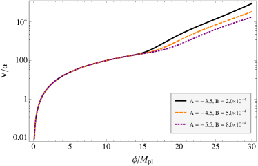
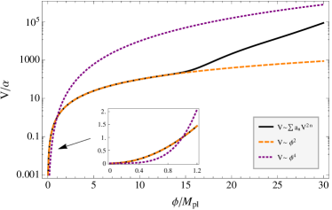
Figure 1: Left: The potential $V$ in Eq.(1) with different parameters $A,B$. Right: Compare to the chaotic inflation models with potentials $V\sim\phi^{2},\phi^{4}$.

From Fig.1, one can see that the potential is increasing with $\phi$ increased, and it gets a little bit more steep when the parameter $A$ becomes small. Compare this potential from Eq.(1) with that in the chaotic inflation, e.g. $\phi^{2}$ or $\phi^{4}$, we find that it could be almost identical to the quadratic one when $\phi$ is small, while it becomes larger than $\phi^{2}$ when $\phi$ goes large, but it is smaller than the quartic potential. Furthermore, one can see that this kind of infinity power series potential is convergent in the physical regions of parameter spaces, which is required for an successful inflation, see Appendix.A.

II.2 Slow-roll parameters

The slow-roll parameters are defined as usual

$$\epsilon=\frac{M_{pl}^{2}}{2}\left(\frac{V^{\prime}}{V}\right)^{2}\,,\quad\eta=M_{pl}^{2}\frac{V^{\prime\prime}}{V}\,,\quad\xi=M_{pl}^{4}\frac{V^{\prime}V^{\prime\prime\prime}}{V^{2}}\,,$$ (6)

where the prime denotes the derivatives with respect to $\phi$. Here we have recovered the unit $M_{pl}$ to indicate these parameters are all dimensionless. By substituting the potential (1) into these definitions, we obtain

$$\epsilon=\frac{1}{2}\phi^{-2}\sum_{n=0}^{\infty}b_{n}\phi^{2n}\,,\quad\eta=\phi^{-2}\sum_{n=0}^{\infty}c_{n}\phi^{2n}\,,\quad\xi=\phi^{-2}\sum_{n=0}^{\infty}d_{n}\phi^{2n}$$ (7)

where $b_{0}=4,c_{0}=2,d_{0}=-B/A$ and $b_{n},c_{n},d_{n}$ (for $n\geq 1$) satisfy the following recurrence relations

$$b_{n} = 4(n+1)a_{n+1}+\sum_{k=1}^{n}\bigg{[}4(k+1)(n-k+1)a_{k+1}a_{n-k+1}-\sum_{m=1}^{k+1}a_{m}a_{k+2-m}b_{n-k}\bigg{]}\,,$$ (8)

$$c_{n} = 2(n+1)(2n+1)a_{n+1}-\sum_{k=1}^{n}a_{k+1}c_{n-k}\,,$$ (9)

$$d_{n} = 8(n+2)(2n+3)(n+1)a_{n+2}$$ (10)

$$+ \sum_{k=1}^{n}\left[8(k+1)(n-k+2)(2n-2k+3)(n-k+1)a_{k+1}a_{n-k+2}-\sum_{m=1}^{k+1}a_{m}a_{k+2-m}d_{n-k}\right]\,.$$

Furthermore, by using the recurrence relation of $a_{n}$ in Eq.(2), we find the following relation between the coefficients of $b_{n},c_{n}$ and $d_{n}$, see Appendix.B for details:

$$(2-B)b_{n}-4c_{n}=4A~{}d_{n}\,,$$ (11)

for $n=0,1,\cdots$. Thus we obtain the relation between the slow-roll parameters

$$\xi=\frac{1}{2A}\bigg{[}(2-B)\epsilon-2\eta\bigg{]}\,.$$ (12)

Furthermore, the number of e-folds before the end of inflation is given by

$$N=\int_{t}^{t_{\text{end}}}Hdt=-\int_{\phi}^{\phi_{\text{end}}}\frac{V}{V^{\prime}}d\phi=\frac{\phi^{2}}{4}\sum_{k=0}^{\infty}\frac{f_{n}}{n+1}(\phi^{2n}-\phi^{2n}_{\rm end})\,,$$ (13)

with $f_{0}=1$ and

$$f_{n}=a_{n+1}-\sum_{k=1}^{n}(k+1)a_{k+1}f_{n-k}\,,$$ (14)

for $n\geq 1$. Here $\phi_{\rm end}$ denotes the value of the inflaton at the end of inflation, which is determined by $\epsilon\approx 1$, or by the following equation:

$$2\phi^{2}_{\rm end}\approx\sum_{n=0}^{\infty}b_{n}\phi_{\rm end}^{2n}\,,$$ (15)

which is around the Planck scale $\phi_{\rm end}/_{M_{pl}}\sim 1$, and one can also numerical solve the above equation for $\phi_{\rm end}$.

II.3 Power spectral index and tensor modes

The power spectrum of the scalar perturbation is given by

$$\mathcal{P}_{s}=A_{s}\left(\frac{k}{k_{*}}\right)^{n_{s}-1+n_{s}^{\prime}\ln(k/k_{*})/2}\,,$$ (16)

where $A_{s}$ is its amplitude, $n_{s}$ is called the spectral index, and $n_{s}^{\prime}=dn_{s}/d\ln k$ is the running of index. In a single field inflation model, the spectral indices and its running could be given in terms of the slow-roll parameters:

$$n_{s}-1 \approx 2\eta-6\epsilon\,,$$ (17)

$$n_{s}^{\prime} \approx 16\epsilon\eta-24\epsilon^{2}-2\xi=16\epsilon\eta-24\epsilon^{2}-A^{-1}\bigg{[}(2-B)\epsilon-2\eta\bigg{]}\,,$$ (18)

where we have used Eq.(12). While the tensor-to-scalar ratio $r$ is simply given by $r\approx 16\epsilon$. Here, one can see the parameter $A,B$ is very important to get a large running of spectral index. From Fig.2, the running of index is in order of $n^{\prime}_{s}\sim\mathcal{O}(\epsilon)\sim\mathcal{O}(10^{-2})$, while the tensor ratio is $r\approx 0.20$. Therefore, both large $r$ and $|n_{s}^{\prime}|$ are realized in the IPS model. The corresponding number of e-folds is $N\approx 35\sim 45$ for $n_{s}\approx 0.96$, which seems enough big to solve the problems in the Big Bang cosmology.

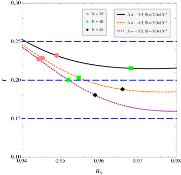
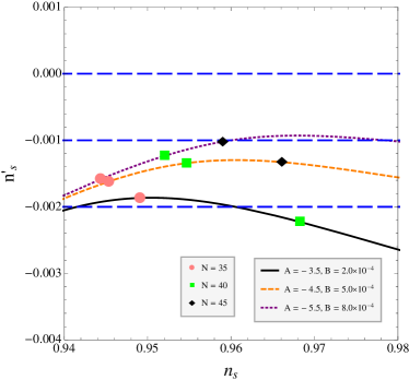
Figure 2: Left: The tensor-to-scalar ratio $r\,\,\,v.s.$ the spectral index $n_{s}$ with parameters $A,B$. Right: The running of the spectral index $n^{\prime}_{s}\,\,\,v.s.$ the spectral index $n_{s}$ with the same parameters.

The latest analysis of the data including the $Planck$ CMB temperature data, the WMAP large scale polarization data (WP) , CMB data extending the Planck data to higher-$l$, the Planck lensing power spectrum, and BAO data gives the constraint on the index $n_{s}$ of the scalar power spectrumAde:2013uln : $0.9583\pm 0.0081$(Planck+ WP), $0.9633\pm 0.0072$ (Planck+WP+lensing), $0.9570\pm 0.0075$ (Planck+WP+highL), $0.9607\pm 0.0063$ (Planck +WP+BAO). It also gives an upper bound on $r\lesssim 0.25$. The BICEP2 experiment constraints the tensor-scalar-ratio as: $r=0.20^{+0.07}_{-0.05}$ in ref.Ade:2014xna . They are also other groups have reported their constrain results on the ratio: $r=0.23^{+0.05}_{-0.09}$ in ref.Cheng:2014ota by adopting the Background Imaging of Cosmic Extragalactic Polarization (B2), Planck and WP data sets; $r=0.20^{+0.04}_{-0.05}$ in ref.Cheng:2014cja combined with the Supernova Legacy Survey (SNLS); $r=0.199^{+0.037}_{-0.044}$ in ref.Li:2014cka by adopting the Planck, supernova Union2.1 compilation, BAO and BICEP2 data sets; and also $r=0.20^{+0.04}_{-0.06}$ in ref.Wu:2014qxa with other BAO data sets. This B-mode signal can not be mimicked by topological defectsLizarraga:2014eaa , and also can not be explained in large extra- dimension models Ho:2014xza . The most likely origin of this signal is from the tensor perturbations or the gravitational wave polarizations during inflation. And also, the cosmological constant seems important during inflation to predict a large tensor modeFeng:2014naa .

By using these results, we obtain the constraints on the parameters $A$ and $B$, see Fig.3. And the value of inflaton field during inflation is typically $\phi/M_{pl}\approx\mathcal{O}(10)$, which corresponds to a large field inflation. By using the amplitude value of the power spectrum from Planck, $A_{s}(k=0.002Mpc^{-1})=2.215\times 10^{-19}$ Ade:2013zuv , we can also estimate the value of the $\alpha$ parameter:

$$\alpha\approx\frac{3\pi^{2}}{2}\left(\sum_{n=1}^{\infty}a_{n}\phi^{2n}\right)^{-1}rA_{s}\approx 4.37\times 10^{-11}\,,$$ (19)

with the best fitting values of $A$ and $B$.

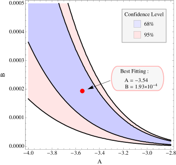
Figure 3: Constraints on the values of parameters $A$ and $B$ with contours from $1\sigma$ to $2\sigma$ confidence levels.

III Conclusion

In this paper, we have proposed the Infinity Power Series (IPS) inflation model with the inflaton potential like Eq.(1). By confronting this model with latest observations from Planck and BICEP2, we constrain the parameters $A$ and $B$. It is found that the absolute value of the running of the spectral index increases with the tensor-to-scalar ratio becomes large, while the number of e-folds is around $35\sim 45$, which seems enough to solve the problems in the Big Bang cosmology, see Fig.2. In a word, the IPS model could predict both a large tensor ratio $r\approx 0.2$ and a large running of spectral index $|n^{\prime}_{s}|\gtrsim\mathcal{O}(10^{-2})$ as well as a large enough number of e-folds, and it also predict the spectral index around $n_{s}\approx 0.96$.

The convergence test has been performed to the inflaton potential in some physical regions of the parameter space. There could be other regions that the potential could be convergent. Furthermore, this kind of potentials could also come from some SUGRA theories, and it deserves further study.

Appendix A Convergence of the inflaton potential

In this section, we will prove that the inflaton potential with infinite power series like Eq.(1) is convergent absolutely in some regions of the parameter space $\{A,B\}$. And within this convergent region, one could get an successful inflation with consistent predictions as described in this paper. First of all, we will prove that the following theorem

Lemma A.1.

By given $(-A)\approx 10^{p},$and $(-B/A)\approx 10^{-2q}$ with $0<p<2q$, then the following equation

$$0\leq a_{n}<\frac{a_{1}B}{8n(2n-1)(n-1)}\left(\frac{B}{-A}\right)^{(n-2)/\beta}\,,$$ (20)

is always valid for $n\geq 2$ as long as $\beta\gtrsim 2q/(q+1)$.

Proof.

By using the recurrence relation (2), we get

$$a_{2}=-\frac{B}{48A}a_{1}\,,\quad a_{3}=\frac{B(B+3)}{5760A^{2}}a_{1}\,,$$ (21)

and both of them satisfy Eq.(20) when $A<-1,B\geq 0$ and $-B/A\ll 1$

$$a_{2}<\frac{B}{48}a_{1}\,,\quad a_{3}<\frac{a_{1}}{240}B\left(\frac{B}{-A}\right)^{1/\beta}$$ (22)

If we assume Eq.(20) is satisfied for $3<m\leq n$, then from Eq.(2) we obtain

$$a_{n+1} = -\frac{1}{8Aa_{1}n(n+1)(2n+1)}\bigg{\{}\sum_{k=1}^{n-2}(n-k)\bigg{[}(6-B)(n-k)-2-(2-B)(n+1)\bigg{]}a_{k+1}a_{n-k}$$ (23)

$$+ 8A\sum_{k=1}^{n-1}(k+1)(n-k+1)(2n-2k+1)(n-k)a_{k+1}a_{n-k+1}+2\left(Bn+2n^{2}-3n+1\right)a_{n}a_{1}\bigg{\}}$$

$$< \frac{a_{1}B}{8(n+1)(2n+1)n}\left(\frac{B}{-A}\right)^{(n-1)/\beta}F(A,B,n)\,,$$

where the function $F$ is given by

$$F(A,B,n)=\frac{1}{8}\bigg{\{}\sum_{k=1}^{n-2}\left(\frac{B}{-A}\right)^{1-2/\beta}\bigg{[}\frac{B}{8k(2k+1)(2n-2k-1)(n-k-1)}-\frac{1}{4(k+1)(2k+1)(2n-2k-1)(n-k-1)}$$ (24)

$$+ \frac{1}{2k(k+1)(2k+1)(2n-2k-1)}\bigg{]}+\left(\frac{B}{-A}\right)^{1-1/\beta}A\sum_{k=1}^{n-1}\bigg{[}\frac{1}{k}-\frac{2}{2k+1}\bigg{]}-\frac{1}{A}\left(\frac{B}{-A}\right)^{-1/\beta}\frac{2}{n}\frac{\left(2n^{2}-3n+1+Bn\right)}{(2n^{2}-3n+1)}\bigg{\}}$$

$$\lesssim \frac{2n-5}{2n-3}10^{-2\left[(q+1)\beta-2q\right]/\beta}-\frac{1}{8}10^{-(2q-p)}\bigg{(}\psi^{(0)}(n)-\psi^{(0)}\left(n+1/2\right)+\gamma+\psi^{(0)}\left(3/2\right)\bigg{)}<1\,.$$

Thus, $a_{n+1}$ also satisfies Eq.(20).

∎

By using this lemma, we perform the Cauchy convergence test on the power series of the potential in Eq.(1)

$$\lim_{n\rightarrow\infty}\left(a_{n}\phi^{2n}\right)^{1/n}<\lim_{n\rightarrow\infty}n^{-3/n}\left(\frac{B}{-A}\right)^{(n-2)/\beta n}\phi^{2}\approx 10^{-(q+1)}\frac{\phi^{2}}{M_{pl}^{2}}<1\,,\quad\text{for}\quad\frac{\phi^{2}}{M_{pl}^{2}}<10^{q+1}\,.$$ (25)

In this paper, we obtain the parameters $(-B/A)\approx 10^{-5}\sim 10^{-6}$ ( or $q\approx 2\sim 3$), and the value of the inflation field during inflation is about $\phi/M_{pl}\lesssim\mathcal{O}(10^{2})$, so the potential is convergent absolutely .

Appendix B Details of the coefficients of the potential

By using the multiplication rules of power series grad ,

$$\sum_{k=0}^{\infty}a_{k}x^{k}\sum_{k=0}^{\infty}b_{k}x^{k}=\sum_{k=0}^{\infty}c_{k}x^{k}\,,\quad c_{n}=\sum_{k=0}^{n}a_{k}b_{n-k}\,,$$ (26)

one can obtain the following relations between the coefficients of $a_{n},b_{n},c_{n}$ and $d_{n}$ from Eqs.(2), (8) -(10)

$$\sum_{n=1}^{\infty}2na_{n}\phi^{2n}\sum_{n=1}^{\infty}2na_{n}\phi^{2n} = \sum_{n=1}^{\infty}a_{n}\phi^{2n}\sum_{n=1}^{\infty}a_{n}\phi^{2n}\sum_{n=0}^{\infty}b_{n}\phi^{2n}\,,$$ (27)

$$\sum_{n=1}^{\infty}2n(2n-1)a_{n}\phi^{2n} = \sum_{n=1}^{\infty}a_{n}\phi^{2n}\sum_{n=0}^{\infty}c_{n}\phi^{2n}\,,$$ (28)

$$\sum_{n=1}^{\infty}2na_{n}\phi^{2n}\sum_{n=1}^{\infty}4n(n+1)(2n+1)a_{n+1}\phi^{2n} = \sum_{n=1}^{\infty}a_{n}\phi^{2n}\sum_{n=1}^{\infty}a_{n}\phi^{2n}\sum_{n=0}^{\infty}d_{n}\phi^{2n}\,.$$ (29)

Multiply Eq.(28) by $4\sum_{n=1}^{\infty}a_{n}\phi^{2n}$, Eq.(29) by $4A$, then subtract the summation of them from Eq.(27) multiplied by $(2-B)$, we finally obtain

$$\sum_{n=1}^{\infty}a_{n}\phi^{2n}\sum_{n=1}^{\infty}a_{n}\phi^{2n}\sum_{n=0}^{\infty}\bigg{[}(2-B)b_{n}-4c_{n}-4Ad_{n}\bigg{]}\phi^{2n}$$ (30)

$$= \sum_{n=1}^{\infty}2na_{n}\phi^{2n}\sum_{n=1}^{\infty}\bigg{[}[2(2-B)n+4]a_{n}-16An(n+1)(2n+1)a_{n+1}\bigg{]}\phi^{2n}-16\sum_{n=1}^{\infty}a_{n}\phi^{2n}\sum_{n=1}^{\infty}n^{2}a_{n}\phi^{2n}\,.$$

Again, by using Eq.(26) and the expression of $a_{n}$ from Eq.(2), one can see that the right hand side of the above equation is indeed vanished. Thus, we obtain the relation (11).

Leading terms of the coefficients of $a_{n},b_{n},c_{n},d_{n}$ and $f_{n}$ with $B=0$ from Eqs.(2), (8)-(10) and (14). Here $a_{1}$ is set to be unity, and $A$ is a parameter in the potential. In the limit of $A\rightarrow\infty$, the only non vanished values of the coefficients are $a_{1}=1,b_{0}=4$ and $c_{0}=2$, which are just the same as the results in the chaotic inflation with a quadratic potential . The relation $(4-B)b_{c}-4c_{n}=4Ad_{n}$ is satisfied for all the values of $n=0,1,\cdots$.

$$a_{1} = +1\,,$$ (31)

$$a_{2} = -\frac{B}{48A}\,,$$ (32)

$$a_{3} = +\frac{B(B+3)}{5760A^{2}}\,,$$ (33)

$$a_{4} = -\frac{B\left(B^{2}+3B+20\right)}{1290240A^{3}}\,,$$ (34)

$$a_{5} = +\frac{B\left(2B^{3}+27B^{2}-177B+420\right)}{928972800A^{4}}\,,$$ (35)

$$a_{6} = -\frac{B\left(2B^{4}-93B^{3}+2319B^{2}-8868B+6048\right)}{490497638400A^{5}}\,,$$ (36)

$$a_{7} = +\frac{B\left(2B^{5}+1293B^{4}-33530B^{3}+212991B^{2}-353652B+110880\right)}{357082280755200A^{6}}\,,$$ (37)

$$a_{8} = -\frac{B\left(2B^{6}-20547B^{5}+665142B^{4}-5886141B^{3}+16998072B^{2}-14707248B+2471040\right)}{342798989524992000A^{7}}\,,$$ (38)

$$\cdots$$

$$b_{0} = 4\,,$$ (39)

$$b_{1} = -\frac{B}{6A}\,,$$ (40)

$$b_{2} = \frac{B(B+8)}{960A^{2}}\,,$$ (41)

$$b_{3} = \frac{B\left(B^{2}+3B-36\right)}{96768A^{3}}\,,$$ (42)

$$b_{4} = \frac{B\left(B^{3}-14B^{2}-96B+160\right)}{11059200A^{4}}\,,$$ (43)

$$b_{5} = \frac{B\left(B^{4}-52B^{3}-12B^{2}+1000B-672\right)}{1362493440A^{5}}\,,$$ (44)

$$b_{6} = \frac{B\left(1382B^{5}-178062B^{4}+1122219B^{3}+2861064B^{2}-10455120B+3628800\right)}{243465191424000A^{6}}\,,$$ (45)

$$b_{7} = \frac{B\left(4B^{6}-1133B^{5}+16482B^{4}-24005B^{3}-126888B^{2}+190224B-38016\right)}{94175546572800A^{7}}\,,$$ (46)

$$\cdots$$

$$c_{0} = 2\,,$$ (47)

$$c_{1} = -\frac{5B}{24A}\,,$$ (48)

$$c_{2} = \frac{B(B+28)}{1920A^{2}}\,,$$ (49)

$$c_{3} = \frac{B\left(2B^{2}+111B-324\right)}{387072A^{3}}\,,$$ (50)

$$c_{4} = \frac{B\left(B^{3}+116B^{2}-996B+880\right)}{22118400A^{4}}\,,$$ (51)

$$c_{5} = \frac{B\left(2B^{4}+545B^{3}-8472B^{2}+21448B-8736\right)}{5449973760A^{5}}\,,$$ (52)

$$c_{6} = \frac{B\left(1382B^{5}+987648B^{4}-22112811B^{3}+104548104B^{2}-123935760B+27216000\right)}{486930382848000A^{6}}\,,$$ (53)

$$c_{7} = \frac{B\left(8B^{6}+16231B^{5}-466176B^{4}+3372995B^{3}-7622088B^{2}+5066640B-646272\right)}{376702186291200A^{7}}\,,$$ (54)

$$\cdots$$

$$d_{0} = -\frac{B}{A}\,,$$ (55)

$$d_{1} = \frac{B(B+3)}{24A^{2}}\,,$$ (56)

$$d_{2} = -\frac{B\left(B^{2}+8B+40\right)}{3840A^{3}}\,,$$ (57)

$$d_{3} = -\frac{B\left(B^{3}+3B^{2}+69B-252\right)}{387072A^{4}}\,,$$ (58)

$$d_{4} = -\frac{B\left(B^{4}-14B^{3}+164B^{2}-1640B+1440\right)}{44236800A^{5}}\,,$$ (59)

$$d_{5} = -\frac{B\left(B^{5}-52B^{4}+637B^{3}-7448B^{2}+18776B-7392\right)}{5449973760A^{6}}\,,$$ (60)

$$d_{6} = -\frac{B\left(1382B^{6}-178062B^{5}+3453639B^{4}-43608996B^{3}+192918960B^{2}-223332480B+47174400\right)}{973860765696000A^{7}}\,,$$ (61)

$$d_{7} = \frac{B\left(-4B^{7}+1133B^{6}-34979B^{5}+523145B^{4}-3294117B^{3}+7178088B^{2}-4648176B+570240\right)}{376702186291200A^{8}}\,,$$ (62)

$$\cdots$$

$$f_{0} = 1\,,$$ (63)

$$f_{1} = \frac{B}{48A}\,,$$ (64)

$$f_{2} = \frac{(B-2)B}{1920A^{2}}\,,$$ (65)

$$f_{3} = \frac{B\left(17B^{2}-89B+60\right)}{1290240A^{3}}\,,$$ (66)

$$f_{4} = \frac{B\left(31B^{3}-285B^{2}+522B-168\right)}{92897280A^{4}}\,,$$ (67)

$$f_{5} = \frac{B\left(691B^{4}-9389B^{3}+31374B^{2}-28620B+5040\right)}{81749606400A^{5}}\,,$$ (68)

$$f_{6} = \frac{B\left(5461B^{5}-99733B^{4}+509592B^{3}-874296B^{2}+462072B-47520\right)}{25505877196800A^{6}}\,,$$ (69)

$$f_{7} = \frac{B\left(1859138B^{6}-43007343B^{5}+304039386B^{4}-817449429B^{3}+838021080B^{2}-278999280B+17297280\right)}{342798989524992000A^{7}}\,,$$

$$\cdots$$ (70)

References

- (1) P. A. R. Ade et al. [BICEP2 Collaboration], arXiv:1403.3985 [astro-ph.CO].
- (2) P. A. R. Ade et al. [Planck Collaboration], arXiv:1303.5082 [astro-ph.CO].
- (3) A. H. Guth, Phys. Rev. D 23, 347 (1981).
- (4) A. D. Linde, Phys. Lett. B 108, 389 (1982).
- (5) A. Albrecht and P. J. Steinhardt, Phys. Rev. Lett. 48, 1220 (1982).
- (6) A. D. Linde, Phys. Lett. B 129, 177 (1983).
- (7) K. Freese, J. A. Frieman and A. V. Olinto, Phys. Rev. Lett. 65, 3233 (1990).
- (8) Y. Gong, arXiv:1403.5716 [gr-qc].
- (9) D. J. H. Chung, G. Shiu and M. Trodden, Phys. Rev. D 68, 063501 (2003) [astro-ph/0305193].
- (10) R. Easther and H. Peiris, JCAP 0609, 010 (2006) [astro-ph/0604214].
- (11) B. Feng, M. Z. Li, R. J. Zhang and X. M. Zhang, Phys. Rev. D 68, 103511 (2003) [astro-ph/0302479].
- (12) T. Kobayashi and F. Takahashi, JCAP 1101, 026 (2011) [arXiv:1011.3988 [astro-ph.CO]].
- (13) K. Nakayama, F. Takahashi and T. T. Yanagida, JCAP 1308, 038 (2013) [arXiv:1305.5099, arXiv:1305.5099 [hep-ph]].
- (14) T. Kobayashi and O. Seto, arXiv:1403.5055 [astro-ph.CO].
- (15) Y. Z. Ma and Y. Wang, arXiv:1403.4585 [astro-ph.CO].
- (16) S. Choudhury and A. Mazumdar, arXiv:1403.5549 [hep-th].
- (17) C. Cheng and Q. G. Huang, arXiv:1403.7173 [astro-ph.CO].
- (18) C. Cheng and Q. G. Huang, arXiv:1404.1230 [astro-ph.CO].
- (19) H. Li, J. Q. Xia and X. Zhang, arXiv:1404.0238 [astro-ph.CO].
- (20) F. Wu, Y. Li, Y. Lu and X. Chen, arXiv:1403.6462 [astro-ph.CO].
- (21) J. Lizarraga, J. Urrestilla, D. Daverio, M. Hindmarsh, M. Kunz and A. R. Liddle, arXiv:1403.4924 [astro-ph.CO].
- (22) C. M. Ho and S. D. H. Hsu, arXiv:1404.0745 [hep-ph].
- (23) C. J. Feng and X. Z. Li, arXiv:1404.3817 [astro-ph.CO].
- (24) P. A. R. Ade et al. [Planck Collaboration], arXiv:1303.5076 [astro-ph.CO].
- (25) I.S. Gradshteyn and I.M. Ryzhik ; Alan Jeffrey, Daniel Zwillinger, editors. Table of Integrals, Series, and Products, seventh edition. Academic Press, 2007. ISBN 978- 0-12-373637-4 .