Numerical simulations of stick percolation: Application to the study of structured magnetorheologial elastomers

Abstract

In this article we explore how structural parameters of composites filled with one-dimensional, electrically conducting elements (such as sticks, needles, chains, or rods) affect the percolation properties of the system. To this end, we perform Monte Carlo simulations of asymmetric two-dimensional stick systems with anisotropic alignments. We compute the percolation probability functions in the direction of preferential orientation of the percolating objects and in the orthogonal direction, as functions of the experimental structural parameters. Among these, we considered the average length of the sticks, the standard deviation of the length distribution, and the standard deviation of the angular distribution. We developed a computer algorithm capable of reproducing and verifying known theoretical results for isotropic networks and which allows us to go beyond and study anisotropic systems of experimental interest. Our research shows that the total electrical anisotropy, considered as a direct consequence of the percolation anisotropy, depends mainly on the standard deviation of the angular distribution and on the average length of the sticks. A conclusion of practical interest is that we find that there is a wide and well-defined range of values for the mentioned parameters for which it is possible to obtain reliable anisotropic percolation under relatively accessible experimental conditions when considering composites formed by dispersions of sticks, oriented in elastomeric matrices.

1 Introduction and Experimental Motivation

Recently, a vigorous interest has arisen in percolating networks built out of nano- and micro-dimensional objects (percolating objects), such as nanotubes and nanowires for various applications such as thin film transistors [1, 2], flexible microelectronics [3], microelectromechanical systems (MEMS) [4, 5], chemical sensors [6], and construction of transparent electrodes for optoelectronic and photovoltaic devices [7, 8]. In particular, if these objects are used as fillers dispersed in an elastomeric polymer and then oriented inside the organic matrix, then there is an anisotropic internal structure to the material. This anisotropic structure can be obtained in practice following different methods, like, for example, orienting the filler particles by means of an external field (electric or magnetic), mechanically squeezing a composite material, etc. A particular case is given by magnetorheological materials, whose mechanical properties can be modified by externally applied magnetic fields. An important example of magnetorheological materials are composites formed by dispersing magnetic filler particles into an elastomer polymeric matrix and then orienting the particles. These materials are referred to as magnetorheological elastomers (MRE). If, additionally, the filler particles are electrically conducting, the MRE may also be a conductor depending on the properties of the filler and matrix materials, and on the conditions of synthesis. A simple procedure to obtain MRE (in film or bulk form) consists of curing the filler-elastomer composite in the presence of a uniform magnetic field, which induces agglomerations of the filler particles into chain-like structures (needles) aligned in the direction of the magnetic field [9, 10, 11, 4].

A desirable property in an electrically conducting MRE is its electrical anisotropy, i.e. its ability to conduct an electrical current preferentially in a special direction. Although we will not tackle here the full problem of the relation between percolation and electrical conductivity, for our current purposes it will suffice to use the fact that there will be a total electrical anisotropy (TEA) in the MRE, i.e. conduction in only a chosen direction, if there are percolating paths formed only in that chosen direction. This direction is given by the preferred orientation of the needles, which coincides with the direction of magnetic field applied during the curing of the material. For example, TEA is a crucial property in devices like extended pressure mapping sensors [4] and Zebra^®-like connectors for parallel flip-chip connections [9]. If the experimental variables are not properly set during the fabrication of the MRE, a material devoid of anisotropy (or with very low anisotropy) might be obtained [9, 4, 12], which would be unsuitable for these types of applications.

The microscopic structure of an MRE film filled with randomly distributed magnetic sticks can be characterized by three parameters: the average length of the sticks, $\langle\ell\rangle$, the standard deviation of the length distribution, $\sigma_{\ell}$, and the standard deviation of the angular distribution, $\sigma_{\theta}$ (around a chosen direction). As will be seen later, in the experimental samples these parameters correspond to a normal distribution for the angle $\theta$ and a log-normal distribution for the length $\ell$. These parameters can be set experimentally by changing the intensity of the magnetic field during the curing, the exposure time to the magnetic field before starting the thermal curing, the viscosity of the matrix, the amount of filler, the magnetic properties of the filler, etc. Two of us have performed several experimental studies of these systems [4, 9, 10], and now we wish to understand how their structural parameters affect the probability of obtaining systems with TEA. Nevertheless, it can be expected that the results of our modeling will also apply to other composite materials with similar internal structure.

In magnetorheological elastomers, micro- or nanoscopic objects (called alternatively chains, needles, or sticks) are formed by magneto-piezo-electric manipulation under appropriate experimental conditions at various stages of the synthesis process [9, 4, 12]. These sticks formed by the filler material can be considered as quasi-one-dimensional objects, so that the nanostructured MRE as a whole can be analyzed in terms of networks of percolating sticks. Percolation can be studied either in bulk (3D) or planar (2D) geometry. For our purposes (i.e. studying the TEA) both situations provide useful models, and we will therefore consider the latter, which allows us to explore numerically larger systems. In rectangular or square MRE films, by definition there is a spanning cluster if there is at least one connecting path between two opposing electrical contacts (located on opposite edges of the film) formed by intersecting sticks. In order to relate electrical conduction to percolation concepts, here we will adopt the criterion that there is TEA if and only if there is a spanning cluster in one direction and not in the other. Thus, we adopt here the well-known two-dimensional model of percolating sticks, which is an example of a continuous percolation model [13, 14, 15, 16, 17, 18, 19, 20] in order to study the dependence of the TEA on the structural parameters $\sigma_{\theta}$, $\langle\ell\rangle$, and $\sigma_{\ell}$. We follow the approach of studying the percolation probability functions in the direction of application of the curing magnetic field and in the orthogonal direction, as functions of the experimental parameters $\sigma_{\theta}$, $\sigma_{\ell}$, and $\langle\ell\rangle$. For this, we have developed a computer algorithm that is able to reproduce and verify known theoretical results for isotropic networks and which allows us to go beyond and study anisotropic systems of experimental interest (for which very limited results are available in the literature. Most available studies deal with square systems, with uniform stick length and uniformly distributed angular anisotropy [2, 13, 21]).

2 Algorithm of Stick-Percolation Simulations

We study two-dimensional stick percolation by means of computer simulations. The percolation probabilities are obtained by repeating a large number of times a percolation experiment (a “realization”). Each experiment consists of, starting with an empty rectangular (sides $L_{x},L_{y}$, aspect ratio $r=L_{x}/L_{y}$) or square (side $L=L_{x}=L_{y}$) box, adding a desired number $\mathscr{N}$ of sticks of length $\ell$ (either a fixed length or statistically distributed values), and determining whether a spanning cluster exists between the vertical and/or horizontal faces of the box. The orientation of a stick is given by an angle $\theta$ with respect to a horizontal axis, also generated randomly, with in general $-\pi\leq\theta\leq\pi$. Depending on the characteristics of the physical system that one wishes to simulate, different statistical distributions for the lengths $\ell$ and the angles $\theta$ can be adopted. For example, the simplest and most usually studied model is the one with a uniform length for all sticks and isotropic angular distribution. Once the sticks of a given realization (our “percolating objects”) have been generated, we need to first determine which sticks intersect. Let $A_{i}$ and $B_{i}$, for $i=1,\ldots,\mathscr{N}$, denote the endpoints of the sticks. For algorithmic purposes, the sticks can be seen as vectors, $\overrightarrow{A_{i}B_{i}}$. Consider a subsystem consisting of only two sticks, $\overrightarrow{A_{1}B_{1}}$ and $\overrightarrow{A_{2}B_{2}}$. It can be demonstrated that they intersect if the following conditions are simultaneously satisfied [22]

$$(\overrightarrow{A_{1}B_{1}}\times\overrightarrow{A_{1}A_{2}})\cdot(\overrightarrow{A_{1}B_{1}}\times\overrightarrow{A_{1}B_{2}})\leq 0,$$

$$(\overrightarrow{A_{2}B_{2}}\times\overrightarrow{A_{2}B_{1}})\cdot(\overrightarrow{A_{2}B_{2}}\times\overrightarrow{A_{2}A_{1}})\leq 0.$$ (1)

The intersection pattern of the $\mathscr{N}$ sticks is explored pairwise with these conditions, and an $\mathscr{N}\times\mathscr{N}$ intersection matrix $J$ is formed such that $J_{ij}=1$ if the sticks $i$ and $j$ intersect, and $J_{ij}=0$ if they do not. The matrix $J$ is then used as the matrix associated to an intersection graph, and a Deep First Search algorithm [23] is implemented to evaluate the presence of spanning clusters connecting the opposite edges of the system. If out of $n$ realizations of the system $k$ of them possess at least one spanning cluster, then $k/n$ is an unbiased estimator of the percolation probability (probability that a system has at least one cluster, referred here as $\wp$), i.e. $k/n\rightarrow\wp$ with $n\rightarrow\infty$. $X\equiv\ k/n$ is a binomially distributed random variable with mean $E[X]=\wp$ an variance $\text{Var}[E]=[\wp\times(1-\wp)]/n$ [24]. Then, for acceptable accuracy (estimator error lower than 2%), at least $10^{3}$ Monte Carlo realizations were performed, yielding comparable or even better statistics than those found in recent studies [2, 21]. We implemented our algorithm in a computer program written in SAGE.

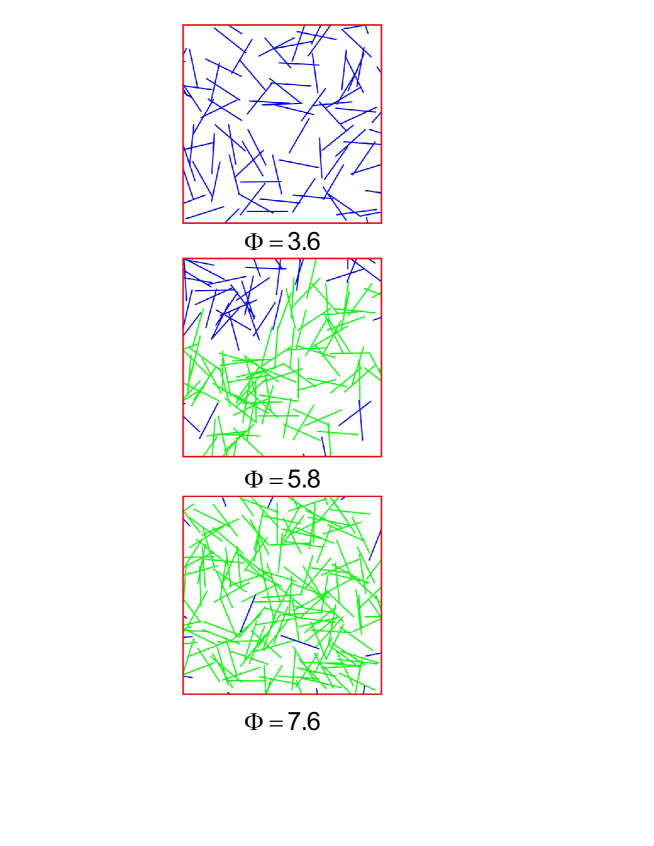
Figure 1: Examples of random stick systems in a square two-dimensional box of side $L=5$ with isotropic angular distribution and stick length $\ell=1$ (all lengths are expressed in the same arbitrary units), for different stick densities. The green (color online) sticks belong to a horizontal spanning cluster and the blue ones do not.

Figure 1 shows three examples of random stick systems in a square two-dimensional box of side $L=5$ with isotropic angular distribution and fixed stick length $\ell=1$ (lengths expressed in the same arbitrary units), for different stick densities, $\Phi=\mathscr{N}/L^{2}$, especially chosen in order to display the percolation behavior, well below, slightly above, and well above the percolation critical density. For the low density there are no spanning clusters. For the described system, for the intermediate density there is one spanning cluster which contains about 60% of the sticks, and for the high density most of the sticks participate in the spanning cluster.

3 Finite-Size Scaling for Square Isotropic Systems

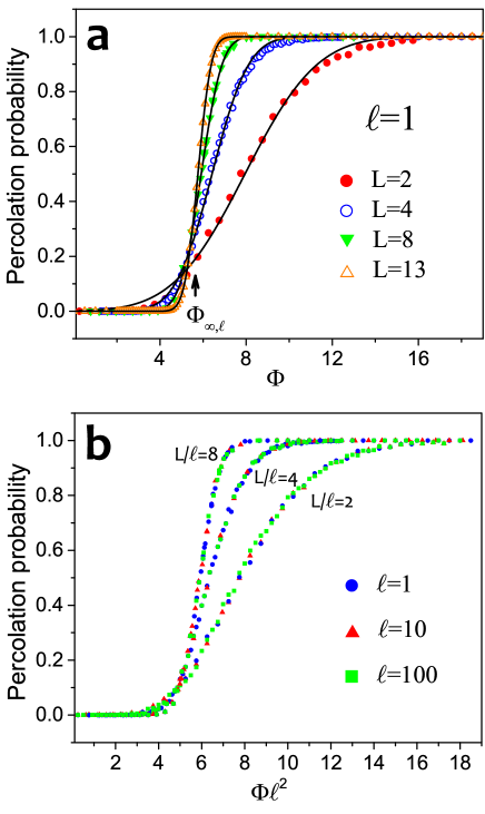
Figure 2: Percolation probability $\wp_{L,\ell}$ for square systems of percolating sticks with isotropic angular distribution. (a) Stick length $\ell=1$; the continuous-line fits assume a Gaussian distribution, Eq. (5). (b) Various values of $L$ and $\ell$, displaying the collapse of data when the percolation probability is plotted against $\Phi\ell^{2}$.

In order to validate our computer-simulation techniques we first reproduce some key scaling results available in the literature on stick percolation for square systems. Let us consider square systems (aspect ratio $r=1$) of side $L$ with $\mathscr{N}$ sticks of fixed length $\ell$. The stick density is thus $\Phi=\mathscr{N}/L^{2}$. The percolation probability $\wp_{L,\ell}(\Phi)$ (i.e. the probability that there is at least one spanning cluster) is shown in Figure 2(a) as a function of $\Phi$ for different values of $L$ and $\ell$. The percolation probability is estimated for each density by running $n>1000$ realizations.

For finite systems, we wish to obtain the critical density $\langle\Phi\rangle_{L,\ell}$, which, according to the Renormalization Group (RG) theory for square systems ($r=1$), scales with the system size $L$ as [17, 25, 16, 26, 14]

$$\langle\Phi\rangle_{L,\ell}=\Phi_{\infty,\ell}+a_{\ell}\,L^{-\frac{1}{\nu}-\vartheta}.$$ (2)

The universal scaling exponent is $\nu=4/3$ for all two-dimensional percolation systems including lattice and continuum percolation (in particular, 2D random sticks systems). Recently it has been found that in random stick percolation square systems ($r=1$) the non-analytical correction given by the exponent $\vartheta$ take the value $0.83\pm 0.02$, consistent with previously published results [27, 28, 29, 30], while in rectangular systems ($r\neq 1$) $\vartheta<0.83$ [16]. From curves like the ones shown in Figure 2(a) one can extract the size-dependent critical percolation density $\langle\Phi\rangle_{L,\ell}$ from the condition

$$\wp_{L,\ell}(\langle\Phi\rangle_{L,\ell})=\frac{1}{2},$$ (3)

which is satisfied if the probability distribution function

$$\Gamma_{L,\ell}(\Phi)=\frac{\partial\wp_{L,\ell}(\Phi)}{\partial\Phi}$$ (4)

is usually assumed to be Gaussian [31, 2]. A quick and rough estimate of the asymptotic critical percolation density $\Phi_{L\rightarrow\infty,\ell}$ (or $\Phi_{\infty,\ell}$) can be obtained by simulating a system with large $L$ and employing Eq. (3). The curve with $L=13$ and $\ell=1$ in Figure 2(a) shows a fairly sharp transition at the critical stick density $\langle\Phi\rangle_{L=13,\ell=1}=5.754$, which is in fairly good agreement with the accepted value of $\Phi_{\infty,\ell=1}=5.6372858(6)$ [26].

A more accurate method to obtain $\langle\Phi\rangle_{L,\ell}$, which also allows us to obtain the standard deviation of the distribution function, $\Delta_{L,\ell}$, consists of fitting the simulated values of $\wp_{L,\ell}$ by a error-function erf($x$) according to Eq. (5)

$$\wp_{L,\ell}(\Phi)=\frac{1}{2}\left[1+\text{erf}\left(\frac{\Phi-\langle\Phi\rangle_{L,\ell}}{\Delta_{L,\ell}}\right)\right],$$ (5)

where $\text{erf}(x)=\frac{2}{\sqrt{\pi}}\int_{0}^{x}e^{-t^{2}}dt$. Excellent fits (R${}^{2}\geq 0.9992$) validating the assumption of Gaussian distribution are displayed in Figure 2(a) as solid lines.

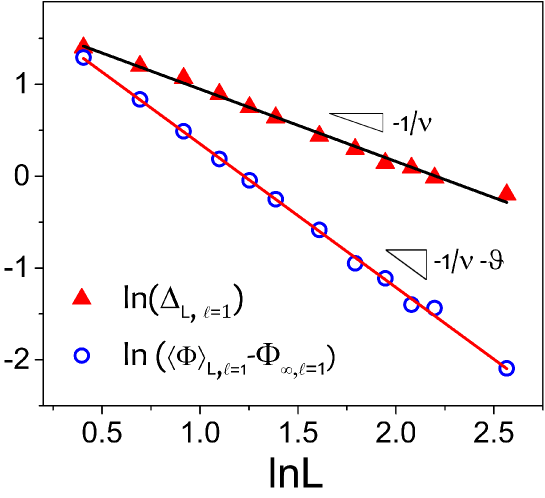
Figure 3: Critical percolation density $\langle\Phi\rangle_{L,\ell}$ and standard deviation $\Delta_{L,\ell}$ versus system size $L$ for square systems with stick length $\ell=1$ (measured in the same units as $L$).

As expected, in Figure 2(a) the percolation transition becomes less sharp for diminishing system size $L$ (according to the RG theory the standard deviation scales as $\Delta_{L,\ell}\propto L^{-1/\nu}$ for isotropic square systems), and at the same time the critical density $\langle\Phi\rangle_{L,\ell}$ shifts towards higher values [Eq. (2)]. Our simulations accurately reproduce the expected scaling laws for the critical density and the standard deviation, as seen in Figure 3 for stick length $\ell=1$. From these curves we obtain $\vartheta=0.83\pm 0.04$ and $\nu=1.33\pm 0.03$ in agreement with previously reported values [27, 28, 16].

The dependence of the percolation probability on the stick length, $\ell$, can be understood thanks to the RG theory, which suggests that there is a relationship between $\Phi_{\infty,\ell}$ and $\ell$ given by the effective area associated to each percolating element. Associating an effective self-area $\ell^{2}$ to each stick, one obtains the relationship [14, 26]

$$\Phi_{\infty,\ell}\ell^{2}=\Phi_{\infty,\ell=1}=5.6372858(6).$$ (6)

Plotting the percolation probability for different values of $\ell$ as a function of $\Phi\ell^{2}$ (instead of doing it simply as a function of $\Phi$) shows that the most relevant quantity is the ratio $L/\ell$ rather than $L$ and $\ell$ independently. In simple terms, this indicates that what matters in the definition of the density of sticks is the system size measured in units of the typical size of the percolating objects. In Figure 2(b) we plot the percolation probability for three values of $\ell=1,10,100$ and corresponding values of the system size $L$ such that $L/\ell=2,4,8$. The excellent collapse of curves with equal ratio $L/\ell$ ratifies the validity of the RG analysis leading to Eq. (6).

4 Synthesis and Experimental Morphological characterization of MRE

The elastomeric material that we studied is comprised of a polydimethylsiloxane (PDMS) polymer matrix and of percolating chains consisting of hybrid magnetite–silver microparticles. These microparticles have an internal structure consisting of clusters of magnetite nanoparticles covered with metallic silver. Using the hybrid filler material described above allows us to obtain a current–conducting magnetorheological material in superparamagnetic state (because magnetite nanoparticles, due to their small diameter, are in a superparamagnetic state at temperatures higher than their blocking temperature, $T_{B}=179\,\text{K}$). The electrical conductivity is not affected by oxidation, given by the chemical fastness of silver metal. Finally, the use of PDMS as polymer matrix increases the chemical resistance of the composite against various chemical agents such as aromatic solvents, halogenated aliphatic solvents, aliphatic alcohols and concentrated salt solutions [4, 9].

The preparation method used to obtain the structured MRE composite with magnetic Fe₃O₄ silver-covered microparticles in PDMS (referred to as PDMS-Fe₃O${}_{4}@$Ag) was described in detail in previous works [4, 9] and is briefly described here. First, Fe₃O₄ superparamagnetic nanoparticles (NPs) were synthesized by the chemical co–precipitation method where a solution mixture (2:1) of FeCl${}_{3}\cdot 6$ H₂O and FeCl${}_{2}\cdot$ 4H₂O in chlorhydric acid was added drop–by–drop to a solution of NaOH ($60\,^{\circ}\mathrm{C}$, pH = 14), under nitrogen atmosphere and high–speed stirring. The obtained nanocrystals were separated by repeated centrifugation and washing cycles, then dried in a vacuum oven at $40\,^{\circ}\mathrm{C}$ during 24 h. The obtained dark brown NPs show a size distribution (determined by TEM images) with maximum at 13 nm in the log–normal distribution of diameters, which is in excellent agreement with the size of the crystallite domains calculated using the Debye–Scherrer relation from X–ray difractograms (XRD), ($14\pm 2$) nm [4, 9, 32, 33].

In a second step, the Fe₃O₄ NPs were covered with silver in order to obtain electrically conductive and superparamagnetic particles. For that, aqueous dispersions of Ag(NH₃)${}_{2}^{+}$ and Fe₃O₄ NPs in a 10:1 molar ratio were sonicated for 30 min at room temperature. Then the system was heated in a water bath at $40\,^{\circ}\mathrm{C}$ for 20 minutes with slow stirring. In the following step, 0.4 M glucose monohydrate solution was added drop–by–drop to the Fe₃O₄–Ag⁺ suspension. Stirring was continued for one hour. This synthesis protocol promotes the reduction of Ag (I) ions adsorbed onto Fe₃O₄ particles. The magnetite–silver particles were separated out from the solution by magnetization and then by centrifugation. After the particles were separated, the decanted supernatant liquid was fully transparent. The obtained system (referred to here as Fe₃O${}_{4}@$Ag) is actually formed by microparticles whose internal structure consists in several Fe₃O₄ nanoparticles clusters covered by metallic silver grouped together. For the Fe₃O${}_{4}@$Ag microparticles (MPs) the maximum of the diameter distribution is at 1.3 $\mu\text{m}$ (determined by SEM and TEM images). For comparison purposes, silver particles (reddish orange) were produced in a separate batch using the same experimental conditions for each set.

Finally polidimethylsoloxane (PDMS) base and curing agent, referred to as PDMS from now on (Sylgard 184, Dow Corning), were mixed in proportions of 10:1 (w/w) at room temperature and then loaded with the magnetic Fe₃O₄ silver-covered microparticles. The amounts of PDMS and fillers were weighed during mixing on an analytical balance, homogenized and placed at room temperature in a vacuum oven for about two hours until the complete absence of any air bubble is achieved. Specifically, composite material with 5% w/w of Fe₃O${}_{4}@$Ag was prepared. The still fluid samples were incorporated into a specially designed cylindrical mould (1 cm diameter by 1.5 cm thickness) and placed in between the magnetic poles of a Varian Low Impedance Electromagnet (model V3703), which provides highly homogeneous steady magnetic fields. The mould was rotated at 30 rpm to preclude sedimentation and heated at $(75\pm 5)\,^{\circ}\mathrm{C}$ in the presence of a uniform magnetic field ($H_{\text{curing}}$= 0.35 T) during 3 hours to obtain the cured material. The polymeric matrix is formed by a tridimensional crosslinked siloxane oligomers network with Si-CH₂-CH₂-Si linkages [34, 35]. Slices of the cured composites were hold in an ad-hoc sample–holder and cut using a sharp scalpel, which were used for the morphological (SEM and optical microscopy analysis) and electrical characterization of material.

All fabricated composites obtained following the procedure described above displayed total electrical anisotropy, showing significant electrical conductivity only in the direction of application of the magnetic field during curing (which coincides with the direction of Fe₃O${}_{4}@$Ag chains). For these MRE materials, electrical resistivity values of $\rho_{\parallel}=4\,\Omega\times\text{cm}$ and $\rho_{\perp}=60\,\text{M}\Omega\times\text{cm}$ were obtained, where $\parallel$ and $\perp$ indicates parallel and perpendicular direction with respect to the filler needles, respectively.

Then, we proceeded to the morphological characterization, evaluating the angular, length, and diameter distributions of the conductive chains. This analysis was performed by computing the angle, length, and diameter of the Fe₃O${}_{4}@$Ag chains in SEM images to several zooms (50x to 6000x) and images obtained by optical microscopy using the image processing software ImageJ v1.47. For SEM images, voltage (EHT) 5 KV and extensions of 100x (3300 pixels.cm-1) and 300x (9800 pixels.cm-1) were typical conditions to compute the average chain length, while to compute chain diameters 3 KV voltages and 4000x (40 pixels.$\mu$m-1) were used.

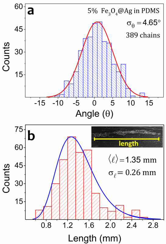
Figure 4: (a) Histogram for the angular distribution of chains in the MRE PDMS-Fe₃O${}_{4}@$Ag 5% w/w. The histogram is adjusted by a Gaussian distribution function (solid line). (b) Histogram associated with the distribution of chain lengths, built by measuring the length of 364 chains. The histogram is adjusted by a log-normal distribution function (solid line). Inset: SEM image of a chain.

Figure 4(a) shows the histogram obtained for the angular distribution of the chains. The histogram is adjusted by a Gaussian distribution function (solid line) centered on the direction of application of the magnetic field during curing $H_{\text{curing}}$ ($\theta=0$) with standard deviation $\sigma_{\theta}=(4.65\pm 0.02)\,^{\circ}$ (count performed on 389 chains).

Figure 4(b) shows the histogram associated with the distribution of chain lengths in the MRE PDMS-Fe₃O${}_{4}@$Ag 5% w/w, built by computing 364 chain lengths. It has an excellent degree of adjustment ($R^{2}=0.9965$) with the log-normal distribution function

$$f_{\lambda}=p\left(\lambda;\langle\lambda\rangle,\sigma_{\lambda}\right)=\frac{1}{\sqrt{2\pi}\sigma_{\lambda}\lambda}\exp{\left(\frac{-[\ln\lambda-\ln\langle\lambda\rangle]^{2}}{2\sigma_{\lambda}^{2}}\right)}$$ (7)

with $\lambda=\ell$ and fitted parameters $\langle\ell\rangle=(1.35\pm 0.01)\,\text{mm}$ y $\sigma_{\ell}=(0.26\pm 0.01)\,\text{mm}$. The average stick density observed is 11.84 needles$/$mm². Note that here, as we start to study concrete physical systems, we begin to use regular units of length, such as millimeters.

The histogram of values of diameters (not shown) was built from 311 counts and also adjusted by a log-normal distribution [Eq. (7) with $\lambda=d$] with an excellent degree of adjustment, $R^{2}=0.9977$, and parameters $\langle d\rangle=(10.40\pm 0.02)\,\mu$m and $\sigma_{d}=(0.30\pm 0.01)\,\mu$m. Note that, under the used experimental conditions, the length of the chain is much greater than its diameter, so that the approximation of one-dimensional percolating elements is justified.

5 Simulation of Anisotropic Systems

From the point of view of possible technological applications of MRE, it is important to characterize the degree of anisotropy of the electrical conductivity of a given device. Anisotropy can be introduced essentially in two ways: through an aspect ratio $r\neq 1$ which makes the system asymmetric (relevant when the characteristic length of the percolating objects is not much smaller than the size of the system, as in our study), and through an anisotropic angular distribution of the sticks. These two aspects can be controlled experimentally in systems like the ones discussed in the previous section, and we will now incorporate them in our simulation studies.

Let us denote the probabilities of having spanning clusters as follows: horizontally $\wp^{H}$, vertically $\wp^{V}$, only horizontally $\wp^{HX}$, only vertically $\wp^{VX}$, on either direction $\wp^{\,U}$, and on both directions $\wp^{HV}$. These probabilities are not independent of each other, as they satisfy $\wp^{\,U}=\wp^{H}+\wp^{V}-\wp^{HV}$ and $\wp^{\,U}=\wp^{HX}+\wp^{VX}+\wp^{HV}$ [26]. The signature of the presence of total anisotropy in the percolation regime will be given by $\wp^{HX}$ taking values very close to 1. Experimentally, a set of parameters that ensure that condition will constitute what we can call a “safety zone” of total anistropic percolation and, therefore, of TEA. The main goal of the present work is to establish a methodology and, with it, to arrive at the specification of such a set of parameter values, as an aid to obtaining TEA in devices that demand it (pressure mapping sensors, bidimensional Zebra^®-like connectors, etc.).

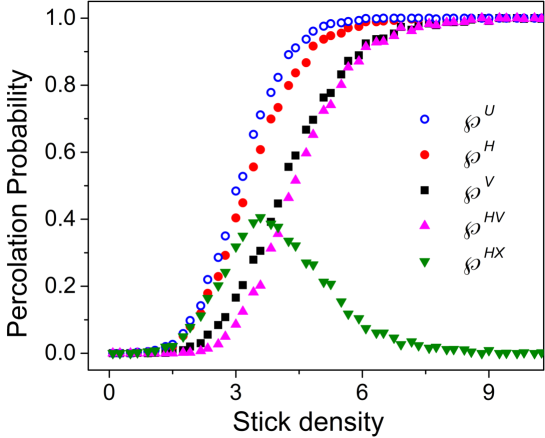
Figure 5: Various percolation probabilities ($\wp^{H},\wp^{V},\wp^{HX},\wp^{\,U},\wp^{HV}$) versus density of sticks ($\text{chains/mm}^{2}$) for a rectangular system of aspect ratio $r=L_{x}/L_{y}=3/4$, $L_{x}=3\,\text{mm}$, and isotropic stick distribution with $\langle\ell\rangle=1.35\,\text{mm}$ and $\sigma_{\ell}=0.26\,\text{mm}$, for a log-normal distribution of stick lengths. Note that $\wp^{VX}$ is not shown since it is always negligible.

It is important to first determine whether the asymmetry of the box or the anisotropy of the angular distribution contribute equally or not to the global anisotropy of the percolation behavior. In Figure 5 we show the percolation probabilities $\wp^{H}$, $\wp^{V}$, $\wp^{HX}$, $\wp^{\,U}$, and $\wp^{HV}$ for a rectangular isotropic (the stick angular distribution is uniform, with $-\pi\leq\theta\leq\pi$) system with aspect ratio $r=3/4$, $L_{x}=3\,\text{mm}$, and log-normal length distribution parameters $\langle\ell\rangle=1.35\,\text{mm}$, and $\sigma_{\ell}=0.26\,\text{mm}$ (notice that $\wp^{VX}$ is negligible and does not need to be considered in the analysis). We remark that these parameters are taken from an experimental sample, as discussed above (Figure 4). The different percolation probabilities verify the expected inequalities $\wp^{\,U}\geq\wp^{H}\geq\wp^{V}\geq\wp^{HV}$, given the chosen asymmetry of the box. The values of $\wp^{HX}$ seen in this figure, never close to unity, indicate that the mere asymmetry of the box ($r\neq 1$) is not enough to produce a safety zone of totally anisotropic conduction. Therefore, we conclude that in order to achieve effective TEA in bulk or films sample geometries it is required to introduce an internal anisotropy, that is, in the stick angular distribution. This conclusion is consistent with experimental observations [4, 9].

We need to introduce a magnitude to characterize in a generic and quantitative way the degree of internal anisotropy of the system of random sticks. Let us denote it macroscopic anisotropy and it will be given by

$$\mathscr{A}=\frac{\sum_{j=1}^{\mathscr{N}}\ell_{j}\left|\cos\theta_{j}\right|}{\sum_{j=1}^{\mathscr{N}}\ell_{j}\left|\sin\theta_{j}\right|}.$$ (8)

In the limit of infinite percolating objects we have $\mathscr{A}=1$ for isotropic systems, while $\mathscr{A}\rightarrow\infty(0)$ for completely anisotropic systems favoring the horizontal (vertical) direction.

5.1 Influence of $\sigma_{\theta}$

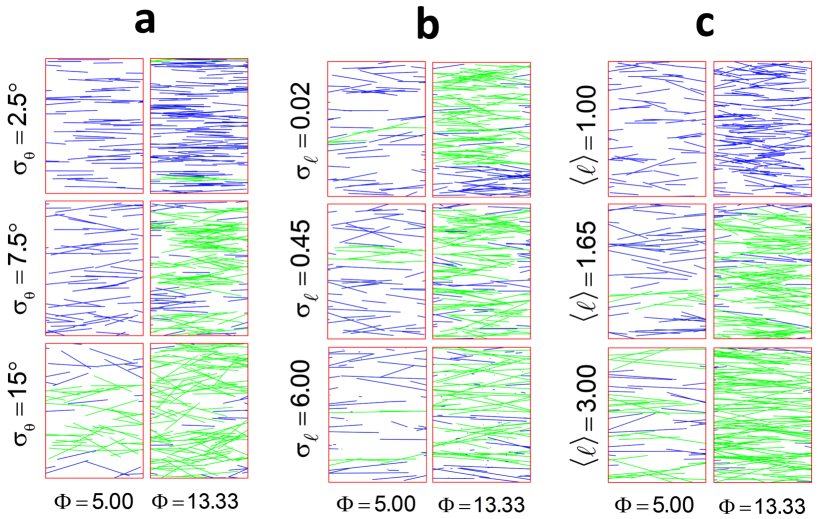
Figure 6: Examples of random stick systems in a two-dimensional box of sides $L_{x}=3\,\text{mm}$ and $L_{y}=4\,\text{mm}$ with anisotropic angular distributions and non-uniform stick length for two different stick densities: $\Phi=5.00\,\text{chains/mm}^{2}$ and $\Phi=13.33\,\text{chains/mm}^{2}$. The green (color online) sticks belong to a horizontal spanning cluster and the blue ones do not. The angle distribution is Gaussian centered in zero, and the length distribution is log-normal (as found experimentally). (a) $\langle\ell\rangle=1.35\,\text{mm}$, $\sigma_{\ell}=0.26\,\text{mm}$, (b) $\langle\ell\rangle=1.35\,\text{mm}$, $\sigma_{\theta}=7.5^{\circ}$ (c) $\sigma_{\theta}=7.5^{\circ}$, $\sigma_{\ell}=0.26\,\text{mm}$.

Figure 6 shows examples of random stick systems in a two-dimensional box of sides $L_{x}=3\,\text{mm}$ and $L_{y}=4\,\text{mm}$ (corresponding to the characteristic dimensions of the experimental samples) with anisotropic angular distributions and non-uniform stick length. In all cases the green sticks belong to a horizontal spanning cluster and the blue ones do not. In particular, Figure 6(a) shows systems for three different values of the standard deviation of the Gaussian angular distribution, $\sigma_{\theta}$, and two values of the stick density $\Phi$, with parameters of a log-normal distribution $\langle\ell\rangle=1.35\,\text{mm}$ and $\sigma_{\ell}=0.26\,\text{mm}$. As expected, for a given value of $\sigma_{\theta}$, more sticks participate in the spanning cluster the higher the density of sticks. We also note that, for a fixed value of the density $\Phi$, the fraction of sticks that belong to the spanning cluster also increases with $\sigma_{\theta}$.

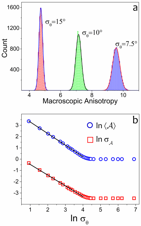
Figure 7: (a) Histograms of the macroscopic anisotropy $\mathscr{A}$ obtained for three different values of $\sigma_{\theta}$ and $\mathscr{N}=1000$ for a rectangular system of aspect ratio $r=L_{x}/L_{y}=3/4$ and anisotropic stick distribution, with parameters of a log-normal distribution $\langle\ell\rangle=1.35\,\text{mm}$ and $\sigma_{\ell}=0.26\,\text{mm}$. (b) Macroscopic anisotropy and its standard deviation versus $\sigma_{\theta}$. For small $\sigma_{\theta}$ we obtain a scaling behavior with exponent approximately equal to $-1$ for both quantities.

To evaluate the effect of $\sigma_{\theta}$, $\langle\ell\rangle$, and $\sigma_{\ell}$ on the TEA (i.e. on the formation of a spanning cluster only in the horizontal direction) numerical simulations of rectangular systems with $L_{x}=3\,\text{mm}$ and $L_{y}=4\,\text{mm}$ ($r=3/4$) were made, taking the horizontal direction ($\theta=0^{\circ}$) as the direction of application of the magnetic field during curing ($H_{\text{curing}}$). In particular, to evaluate the effect of $\sigma_{\theta}$, a log-normal distribution for the lengths with parameters $\langle\ell\rangle=1.35\,\text{mm}$ and $\sigma_{\ell}=0.26\,\text{mm}$ (empirical parameters for the MRE PDMS-Fe₃O₄@Ag 5% w/w), and a Gaussian angular distribution with parameters $\langle\theta\rangle=0^{\circ}$ and different values of standard deviation, $\sigma_{\theta}$, were used in our simulations. Figure 7(a) shows histograms of macroscopic anisotropy, $\mathscr{A}$ obtained for three different values of $\sigma_{\theta}$ ($15^{\circ}$, $10^{\circ}$, and $7.5^{\circ}$), each one obtained by performing 10500 repetitions, with $\mathscr{N}=1000$. For all values of $\sigma_{\theta}$, the distribution is approximately Gaussian, with an excellent degree of fitting, $R^{2}\geq 0.99926$ [continuous-line in Figure 7(a)]. For these distributions, the average macroscopic anisotropy, $\langle\mathscr{A}\rangle$, and its standard deviation, $\sigma_{\mathscr{A}}$, follow a monotonously decreasing behavior with $\sigma_{\theta}$, as illustrated in Figure 7(b). It is noteworthy that for small values of $\sigma_{\theta}$ ($\sigma_{\theta}<55^{\circ}$) there exists a linear relationship between $\ln\langle\mathscr{A}\rangle$ and $\ln\sigma_{\theta}$, as well as between $\ln\sigma_{\mathscr{A}}$ and $\ln\sigma_{\theta}$ [solid lines in Figure 7(b), with $R^{2}=0.9998$, slope = -1.02(7) and intercept= 4.32(1) for $\ln\langle\mathscr{A}\rangle$, and $R^{2}=0.99897$, slope = -0.97(6), and intercept = 0.48(3) for $\ln\sigma_{\mathscr{A}}$].

As described above, a strategy to study the influence of $\sigma_{\theta}$ on the TEA of the composite material is to evaluate curves of $\wp^{HX}(\Phi)$ for different values of $\sigma_{\theta}$. Values of $\Phi$ for which $\wp^{HX}(\Phi)=1$ (if they exist) constitutes ’safety zones’ in terms of TEA: for fixed values of $\langle\ell\rangle$, $\sigma_{\ell}$, $\sigma_{\theta}$, and densities of percolating objects $\Phi$ in this ’safety zone’, systems are most likely to have TEA, i.e. electrical conductivity only in the horizontal direction by formation of a spanning cluster only in that direction.

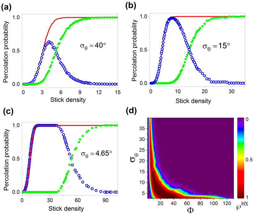
Figure 8: Various percolation probabilities ($\wp^{H},\wp^{V},\wp^{HX}$) versus density of sticks for a rectangular system of aspect ratio $r=L_{x}/L_{y}=3/4$ and anisotropic stick distribution, with parameters of a log-normal distribution $\langle\ell\rangle=1.35\,\text{mm}$ and $\sigma_{\ell}=0.26\,\text{mm}$. (a)-(c) Three different values of the standard deviation $\sigma_{\theta}$ of the angular Gaussian distribution. Red solid line: $\wp^{H}$, green filled circles: $\wp^{V}$, blue open circles: $\wp^{HX}$. (d) Probability $\wp^{HX}$ as a contour plot versus the stick density $\Phi$ and $\sigma_{\theta}$, showing the full dependence on $\sigma_{\theta}$ not seen in the other panels.

Figure 8(a-c) show the curves of $\wp^{H},\wp^{V}$, and $\wp^{HX}$, for three values of $\sigma_{\theta}$ ($40^{\circ}$, $15^{\circ}$ and $4.65^{\circ}$) for systems with log-normal distribution for the stick lengths with parameters $\langle\ell\rangle=1.35\,\text{mm}$ and $\sigma_{\ell}=0.26\,\text{mm}$. There are values of $\Phi$ for which $\wp^{HX}(\Phi)=1$ only when $\sigma_{\theta}<15^{\circ}$. Such behavior of $\wp^{HX}(\Phi)$ is detailed in Figure 8(d), which shows the probability $\wp^{HX}(\Phi)$ as a contour plot of density versus $\Phi$ and $\sigma_{\theta}$. It can be seen that the range of values of $\Phi$ for which $\wp^{HX}(\Phi)=1$ strongly increases with decreasing $\sigma_{\theta}$ and, also, with lower values of the parameter $\sigma_{\theta}$ higher stick density $\Phi$ is required to reach the safety zone.

As described in Section 4, all the PDMS-Fe₃O₄@Ag 5%w/w systems synthesized have $\Phi=11.84\,\text{chains/mm}^{2}$ and electrical anisotropy (measurable electrical conductivity only in the direction of the magnetic field applied during the curing of the material). Panel (c) of Figure 8 shows that, for this value of $\Phi$ and the parameters $\sigma_{\theta}=4.65^{\circ}$, $\langle\ell\rangle=1.36\,\text{mm}$ and $\sigma_{\ell}=0.26\,\text{mm}$ (experimental parameters for PDMS-Fe₃O₄@Ag 5%w/w), we have a very high only-horizontally percolation probability, which shows a very good correlation between our performed simulations and the experimental results obtained.

5.2 Influence of $\sigma_{\ell}$

Following a similar procedure to the one described in the previous section, in order to evaluate the effect of $\sigma_{\ell}$, a Gaussian angular distribution with parameters $\langle\theta\rangle=0^{\circ}$ and $\sigma_{\theta}=7.5^{\circ}$, and a log-normal distribution for the lengths with parameters $\langle\ell\rangle=1.35\,\text{mm}$ and different values of $\sigma_{\ell}$ were used in our simulations. Figure 6(b) shows systems for three different values of the standard deviation of the log-normal length distribution, $\sigma_{\ell}$, and two values of the stick density $\Phi$, with structural parameters $\langle\ell\rangle=1.35\,\text{mm}$ and $\sigma_{\theta}=7.5^{\circ}$.

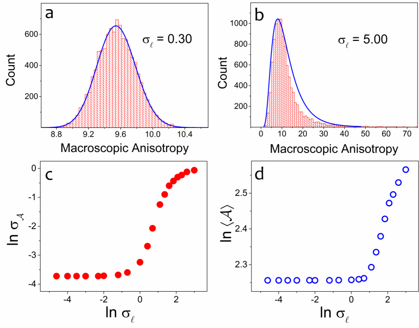
Figure 9: (a,b) Histograms of the macroscopic anisotropy $\mathscr{A}$ obtained for two different values of $\sigma_{\ell}$ and $\mathscr{N}=1000$ for a rectangular system of aspect ratio $r=L_{x}/L_{y}=3/4$ and parameters $\langle\ell\rangle=1.35\,\text{mm}$ and $\sigma_{\theta}=7.5^{\circ}$. (c,d) Macroscopic anisotropy and its standard deviation versus $\sigma_{\ell}$.

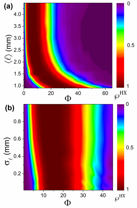
Figure 10: Probability $\wp^{HX}$ as a contour plot versus the stick density $\Phi$ and (a) $\langle\ell\rangle$ with $\sigma_{\theta}=7.5^{\circ}$ and $\sigma_{\ell}=0.26\,\text{mm}$ (b) $\sigma_{\ell}$ with $\langle\ell\rangle=1.35\,\text{mm}$ and $\sigma_{\theta}=7.5^{\circ}$.

Figure 9 shows histograms of macroscopic anisotropy $\mathscr{A}$ obtained for two different values of $\sigma_{\ell}$ (0.30 mm and 5.00 mm), each one obtained by performing 10500 repetitions, with $\mathscr{N}=1000$. For all the values of $\sigma_{\ell}$, the distribution is approximately log-normal, with an excellent degree of adjustment, $R^{2}\geq 0.99511$ [continuous-line in Figure 9(a-b)]. At low values of $\sigma_{\ell}$ the distribution is approximately Gaussian. For these distribution, the average macroscopic anisotropy, $\mathscr{A}$, and its standard deviation, $\sigma_{\mathscr{A}}$, follow a monotonous increasing behavior with $\sigma_{\ell}$, as illustrated in Figure 9(c-d). Again, the strategy that we use to study the influence of $\sigma_{\ell}$ on the electrical anisotropy of the composite material is to evaluate curves of $\wp^{HX}(\Phi)$ for different values of $\sigma_{\ell}$. Figure 10(b) shows the probability $\wp^{HX}(\Phi)$ as a contour plot versus $\Phi$ and $\sigma_{\ell}$. It can be seen that the range of values of $\Phi$ for which $\wp^{HX}(\Phi)\approx 1$ varies very little with the studied parameter. Only a small increase with increasing $\sigma_{\ell}$ from 0 mm to 1 mm is observed. Above those values (not shown) practically no variation with $\sigma_{\ell}$ is observed, and therefore the location and size of the safety zone becomes quite insensitive to $\sigma_{\ell}$.

5.3 Influence of $\langle\ell\rangle$

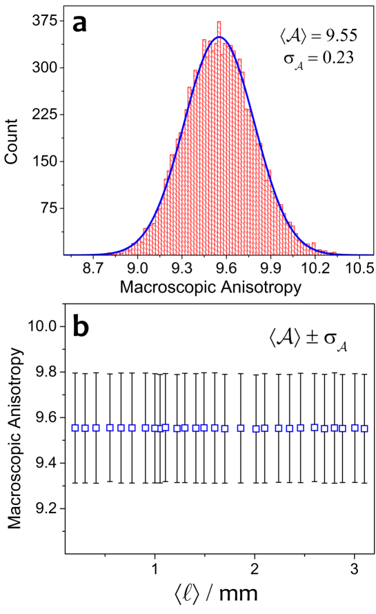
Figure 11: (a) Typical histogram of the macroscopic anisotropy $\mathscr{A}$ obtained for a rectangular system of aspect ratio $r=L_{x}/L_{y}=3/4$, $\mathscr{N}=1000$, and parameters $\sigma_{\theta}=7.5^{\circ}$ and $\sigma_{\ell}=0.26\,\text{mm}$. (b) Mean value of macroscopic anisotropy and its standard deviation versus $\langle\ell\rangle$.

In this case, a Gaussian angular distribution with parameters $\langle\theta\rangle=0^{\circ}$ and $\sigma_{\theta}=7.5^{\circ}$, and a log-normal distribution for the lengths with parameters $\sigma_{\ell}=0.26\,\text{mm}$ and different values of $\langle\ell\rangle$ were assumed. Figure 10(a) shows the probability $\wp^{HX}(\Phi)$ as a contour plot versus $\Phi$ and $\langle\ell\rangle$. It can be seen that the range of values of $\Phi$ for which $\wp^{HX}(\Phi)\approx 1$ varies very little with the studied parameter but the value of $\Phi$ required to reach the safety zone strongly increases with decreasing $\langle\ell\rangle$. Figure 11(a) shows a typical macroscopic anisotropy histogram obtained for $\langle\ell\rangle=1.22\,\text{mm}$ by performing 10500 repetitions, with $\mathscr{N}=1000$. For all the values of $\langle\ell\rangle$, the distribution is approximately Gaussian, with an excellent degree of adjustment, $R^{2}\geq 0.99977$ [continuous-line in Figure 11(a)]. Contrary to what was observed for the other two structural parameters, in this case the histograms do not change appreciably for different values of $\langle\ell\rangle$, as can be clearly seen in Figure 11(b), in which mean values of macroscopic anisotropy and its standard deviation are plotted versus $\langle\ell\rangle$.

6 Conclusions

Motivated by experimental work on structured magnetorheologial elastomers, we present a comprehensive study of stick percolation in two dimensional networks. In order to extract realistic parameters for our simulations, we first carry out a statistical characterization of the distribution of metallic sticks in our previously studied MRE samples. We found that the population of sticks has a log-normal distribution of stick lengths (centered around $1.35\,\text{mm}$) and a Gaussian angular distribution. The latter is centered around a preferential axis that is given by the curing magnetic field applied during the sample preparation, and has a typical standard deviation of approximately five degrees. In order to simulate the experimental systems, we adopted the model of two-dimensional stick percolation and developed a Monte Carlo numerical algorithm and a computer program implemented in the computer language SAGE. We thoroughly tested our program by reproducing theoretical key results of the known scaling behavior of the percolation probability in square, isotropically distributed systems. We then performed extensive numerical simulations of asymmetric (rectangular), anisotropic (in the orientation of the sticks) systems, modeled after the examined experimental samples. The main objective of the study was to analyze the effect of key structural parameters of the material, which characterize the angular and length distribution of the sticks (the average length of the sticks $\langle\ell\rangle$, the standard deviation of the length distribution $\sigma_{\ell}$, and the standard deviation of the angular distribution $\sigma_{\theta}$) on the observation of total electrical anisotropy (TEA). From a practical point of view, TEA is a crucial aspect in the design of nano or micro-scale devices like pressure mapping sensors and two-dimensional aniso connectors (e.g. Zebra^®-like connectors for parallel flip-chip connections). We studied the TEA by computing various probabilities, especially the only-horizontal probability percolation function, $\wp^{HX}$, and analyzing the macroscopic anisotropy, which quantifies the macrosocpic average degree of orientation of the stick population. We find prescriptions to achieve “safe” structural conditions of total electrical anisotropy, and thus hope to guide the experimentalist and technologist to choose the experimental conditions needed to make a device with the desired electrical properties. Most importantly, we show that there exists a strong dependence of the TEA on the standard deviation of the angular distribution and on the average length of the sticks, while the standard deviation of the length distribution has little effect.

RMN and PIT are research members of the National Council of Research and Technology (CONICET, Argentina). Financial support was received from UBA (UBACyT projects 2012-2015, number 20020110100098 and 2011-2014 number 20020100100741), and from the Ministry of Science, Technology, and Innovation (MINCYT-FONCYT, Argentina, PICT 2011-0377). Support from the Center of Documental Production (CePro) and the Center of Advanced Microscopy (CMA) (FCEyN, UBA) to obtain the shown SEM-TEM images and from the Low-Temperatures Laboratory (Department of Physics, FCEyN, UBA) to implement the device used to generate the structured materials is gratefully acknowledged. We thank the SAGE users community for fruitful discussions and Prof. William Stein (University of Washington) for allowing us to run some of our simulations on SageMathCloud.

References

- [1] Gupta, M. P., Behnam, A., Lian, F., Estrada, D., Pop, E., and Kumar, S., Nanotechnology 24, 405204 (2013).
- [2] Zeng, X., Xu, X., Shenai, P. M., Kovalev, E., Baudot, C., Mathews, N., and Zhao, Y., J. Phys. Chem. C 115, 21685–21690 (2011).
- [3] Kocabas, C., Meitl, M. A., Gaur, A., Shim, M., and Rogers, J. A., Nano Lett. 4, 2421–2426 (2004).
- [4] Mietta, J. L., Jorge, G., Perez, O. E., Maeder, T., and Negri, R. M., Sens. Actuators Phys. 192, 34–41 (2013).
- [5] Snow, E. S., Campbell, P. M., Ancona, M. G., and Novak, J. P., Appl. Phys. Lett. 86, 033105 (2005).
- [6] Collins, P. G., Bradley, K., Ishigami, M., and Zettl, A., Science 287, 1801–1804 (2000).
- [7] Hicks, J., Behnam, A., and Ural, A., Phys. Rev. E 79, 012102 (2009).
- [8] Pasquier, A. D., Unalan, H. E., Kanwal, A., Miller, S., and Chhowalla, M., Appl. Phys. Lett. 87, 203511 (2005).
- [9] Mietta, J. L., Ruiz, M. M., Antonel, P. S., Perez, O. E., Butera, A., Jorge, G., and Negri, R. M., Langmuir 28, 6985–6996 (2012).
- [10] Antonel, P. S., Jorge, G., Perez, O. E., Butera, A., Leyva, A. G., and Negri, R. M., J. Appl. Phys. 110, 043920–043920–8 (2011).
- [11] Kchit, N. and Bossis, G., J. Phys. Condens. Matter 20, 204136 (2008).
- [12] Boczkowska, A. and Awietj, S., Microstructure and Properties of Magnetorheological Elastomers. In Advanced Elastomers—Technology, Properties and Applications; Boczkowska, A., Ed.; InTech, 2012.
- [13] Yook, S.-H., Choi, W., and Kim, Y., J. Korean Phys. Soc. 61, 1257–1262 (2012).
- [14] Li, J. and Zhang, S.-L., Phys. Rev. E 80, 040104 (2009).
- [15] Kim, Y., Yun, Y., and Yook, S.-H., Phys. Rev. E 82, 061105 (2010).
- [16] Žeželj, M., Stanković, I., and Belić, A., Phys. Rev. E 85, 021101 (2012).
- [17] Introduction to Percolation Theory, Stauffer, D. and Aharony, A. (Taylor & Francis, 1992).
- [18] Matoz-Fernández, D. A., Linares, D. H., and Ramírez-Pastor, A. J., Eur. Phys. J. B 85, 1–7 (2012).
- [19] Ambrosetti, G., Grimaldi, C.,Balberg, I., Maeder, T., Danani, A., and Ryser, P., Phys. Rev. B 81, 155434 (2010).
- [20] Nigro, B., Grimaldi, C., Ryser, P., Chatterjee, A. P., and van der Schoot, P., Phys. Rev. Lett. 110, 015701 (2013).
- [21] Lin, K. C., Lee, D. An, L. and Joo, Y. H. Nanosci. Nanoeng. 1, 15–22 (2013).
- [22] Computational Geometry: Algorithms and Applications, Mark de Berg, Otfried Cheong, Marc van Kreveld (Springer, 2008).
- [23] Distributed Graph Algorithms for Computer Networks, Erciyes, K. (Springer, 2013).
- [24] Probability and Statistics for Engineering and the Sciences, Dvore, J.Ł. (Cengage Learning, 2012).
- [25] Hovi, J.-P. and Aharony, A., Phys. Rev. E 53, 235–253 (1996).
- [26] Mertens, S. and Moore, C., Phys. Rev. E 86, 061109 (2012).
- [27] Ziff, R. M. and Newman, M. E. J., Phys. Rev. E 66, 016129 (2002).
- [28] Ziff, R. M., Phys. Rev. Lett. 69, 2670–2673 (1992).
- [29] Aharony, A. and Hovi, J.-P., Phys. Rev. Lett. 72, 1941–1941 (1994);
- [30] Stauffer, D., Phys. Lett. A 83, 404–405 (1981).
- [31] Rintoul, M. D. and Torquato, S., J. Phys. Math. Gen. 30, L585 (1997).
- [32] Godoy, M., Moreno, A. J., Jorge, G. A., Ferrari, H. J., Antonel, P. S., Mietta, J. L., Ruiz, M., Negri, R. M., Pettinari, M. J., and Bekeris, V., J. Appl. Phys. 111, 044905 (2012).
- [33] Butera, A., Álvarez, N., Jorge, G., Ruiz, M. M., Mietta, J. L., and Negri, R. M., Phys. Rev. B 86, 144424 (2012).
- [34] Efimenko, K., Wallace, W. E., and Genzer, J., J. Colloid Interface Sci. 254, 306–315 (2002).
- [35] Esteves, A. C. C., Brokken–Zijp, J., Laven, J., Huinink, H. P., Reuvers, N. J. W., Van, M. P., and G. de With, Polymer 50, 3955–3966 (2009).