Throughput-Optimal Scheduling Design with Regular Service Guarantees in Wireless Networks thanks: Bin Li (celibin@gmail.com), Ruogu Li (lirg03@gmail.com), and Atilla Eryilmaz (eryilmaz.2@osu.edu) are with the Department of Electrical and Computer Engineering at The Ohio State University, Columbus, Ohio 43210 USA.

Bin Li, Ruogu Li, and Atilla Eryilmaz
Abstract

Motivated by the regular service requirements of video applications for improving Quality-of-Experience (QoE) of users, we consider the design of scheduling strategies in multi-hop wireless networks that not only maximize system throughput but also provide regular inter-service times for all links. Since the service regularity of links is related to the higher-order statistics of the arrival process and the policy operation, it is highly challenging to characterize and analyze directly. We overcome this obstacle by introducing a new quantity, namely the time-since-last-service (TSLS), which tracks the time since the last service. By combining it with the queue-length in the weight, we propose a novel maximum-weight type scheduling policy, called Regular Service Guarantee (RSG) Algorithm. The unique evolution of the TSLS counter poses significant challenges for the analysis of the RSG Algorithm.

To tackle these challenges, we first propose a novel Lyapunov function to show the throughput optimality of the RSG Algorithm. Then, we prove that the RSG Algorithm can provide service regularity guarantees by using the Lyapunov-drift based analysis of the steady-state behavior of the stochastic processes. In particular, our algorithm can achieve a degree of service regularity within a factor of a fundamental lower bound we derive. This factor is a function of the system statistics and design parameters and can be as low as two in some special networks. Our results, both analytical and numerical, exhibit significant service regularity improvements over the traditional throughput-optimal policies, which reveals the importance of incorporating the metric of time-since-last-service into the scheduling policy for providing regulated service.

I Introduction

During the past years, there has been increasing deployment of a variety of real-time applications over the wireless networks, especially streaming multi-media applications. Unlike its non-real-time counterpart, the real-time traffic often has various quality-of-service (QoS) requirements besides throughput. Such requirements usually include end-to-end delay constraints, packet delivery ratio requirements, and the regularity of the inter-service times. Unlike the traditional long-term mean throughput based requirements, these QoS requirements often have a complex dependence on the higher-order statistics of the arrival process as well as the system operation. Thus, the canonical optimization-based approaches that aim to optimize the throughput performance (e.g., [24, 4, 15, 19, 16]) do not apply.

Recently, valuable efforts have been exerted in the design of algorithms that improve various aspects of the QoS, especially on the delay performance of the algorithms. For example, some works focus on designing algorithms with low end-to-end delay performance, such as [1, 27, 25]. Constant delay bounds (e.g. [17]) and delivery ratio requirements for deadline-constrained traffic (e.g. [7, 8, 9, 10, 12]) are some of the other QoS metrics considered in the literature.

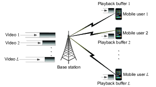
However, these QoS metrics do not fully characterize the Quality-of-Experience (QoE) of users in video applications in wireless networks. To see it, we can envision the network scenario where each individual user wants to download its video from the base station, as shown in Fig. 1.
Refer to caption
Figure 1: Cellular network with a single base station and L𝐿L users

Each mobile user would like to receive the data from the base station regularly. Indeed, the QoE of users is highly related to the average Perceived Video Quality (PVQ) across the sequence of scenes forming the video, where the PVQ traditionally is a local quality measure associated with a particular scene or a short period of time. In [26, 11], the authors point out that the variance in PVQ leads to the worse QoE than the constant quality video with even smaller average PVQ. Yet, both the time-varying nature of wireless channels and the scheduling policy significantly affect the variance of the received data of each mobile user. Traditional scheduling policies aiming to maximize the system throughput or minimize the delay at the base station side do not take users’ experience into account and thus lead to the high variance of the received data of mobile users.

This motivates us to reduce variability of arrivals to the mobile users, which can be achieved by providing regulated inter-service times for the arriving flows at the base station end. However, the inter-service time characteristics are difficult to analyze directly due to: its complex dependence on the high-order statistics of the arrival and service processes, and its non-Markovian evolution. To overcome this, we need to find new approaches to study the inter-service time behavior. To the best of our knowledge, this is the first work that rigorously studies the service regularity of the scheduling policies. Our contributions in this work can be summarized as follows:

\bullet We introduce a new quantity (cf. Section II), namely the time-since-last-service, that has a tight relationship with the service regularity performance, and hence enables novel design strategies. Yet, this new parameter has its unique evolution, drastically different from a queue, which poses new challenges for its analysis.

\bullet We develop a novel maximum-weight type scheduling policy that combines the time-since-last-service parameter and the queue-length in its weight measure (cf. Section III). Then, we show that the proposed scheduling policy possesses the desirable throughput optimality property by using a novel Lyapunov function.

\bullet We derive lower and upper bounds on the service regularity performance (cf. Section IV) by utilizing a novel Lyapunov-drift-based argument, inspired by the approach in [3]. We further show that, by properly scaling the design parameter in our policy, we can guarantee a degree of service regularity within a factor of our fundamental lower bound. This factor is a function of the system statistics and design parameters and can be as low as two under symmetric arrival rates in some special networks.

\bullet We support our analytical results with extensive numerical investigations (cf. Section V), which show significant performance gains in the service regularity over the traditional queue-length-based policies. Furthermore, the numerical investigations indicate that the service regularity performance of our policy actually approaches the lower bounds as the weight of the time-since-last-service increases in some special networks.

This work extends our earlier work [14] in several key aspects: (1) we conduct novel analyses that extend both throughput optimality and service regularity guarantee results to general multi-hop fading networks; (2) we show the existence of all moments of the system state under our proposed algorithm, which establishes the foundation to utilize the Lyapunov-drift based analysis of the steady-state behavior of stochastic processes; (3) we conduct simulations to compare our policy with traditional queue-length-based scheduling algorithms in more general setups, including switch topologies and fading scenarios.

II system model

We consider a wireless network with L𝐿L links, where a link represents a pair of a transmitter and a receiver that are within the transmission range of each other. We assume that the system operates in slotted time with normalized slots t{1,2,}𝑡12t\in\{1,2,...\}. Due to the interference-limited nature of wireless transmissions, the success or failure of a transmission over a link depends on whether an interfering link is also active in the same slot, which is called the link-based conflict model. We call a set of links that can be active simultaneously as a feasible schedule and denote it as 𝐒[t]=(Sl[t])l=1L𝐒delimited-[]𝑡superscriptsubscriptsubscript𝑆𝑙delimited-[]𝑡𝑙1𝐿\mathbf{S}[t]=(S_{l}[t])_{l=1}^{L}, where Sl[t]=1subscript𝑆𝑙delimited-[]𝑡1S_{l}[t]=1 if the link l𝑙l is scheduled in slot t𝑡t and Sl[t]=0subscript𝑆𝑙delimited-[]𝑡0S_{l}[t]=0, otherwise. We use 𝒮𝒮\mathcal{S} to denote the set of all feasible schedules.

We capture the channel fading over link l𝑙l via a non-negative-integer-valued random variable Cl[t]subscript𝐶𝑙delimited-[]𝑡C_{l}[t], with Cl[t]Cmaxsubscript𝐶𝑙delimited-[]𝑡subscript𝐶C_{l}[t]\leq C_{\max}, l,tfor-all𝑙𝑡\forall l,t, for some Cmax<subscript𝐶C_{\max}<\infty, which measures the maximum amount of service available in slot t𝑡t, if the link l𝑙l is scheduled. We assume that 𝐂[t]=(Cl[t])l=1L𝐂delimited-[]𝑡superscriptsubscriptsubscript𝐶𝑙delimited-[]𝑡𝑙1𝐿\mathbf{C}[t]=(C_{l}[t])_{l=1}^{L}, t0for-all𝑡0\forall t\geq 0, are independently and identically distributed (i.i.d.) over time. We assume that c¯minminl𝔼[Cl[t]]>0subscript¯𝑐subscript𝑙𝔼delimited-[]subscript𝐶𝑙delimited-[]𝑡0\overline{c}_{\min}\triangleq\min_{l}\mathds{E}[C_{l}[t]]>0. Let 𝒮(𝐜){𝐒𝐜:𝐒𝒮}superscript𝒮𝐜conditional-set𝐒𝐜𝐒𝒮\mathcal{S}^{(\mathbf{c})}\triangleq\{\mathbf{S}\mathbf{c}:\mathbf{S}\in\mathcal{S}\} denote the set of feasible rate vectors when the channel is in state 𝐜𝐜\mathbf{c}, where 𝐚𝐛=(albl)l=1L𝐚𝐛superscriptsubscriptsubscript𝑎𝑙subscript𝑏𝑙𝑙1𝐿\mathbf{a}\mathbf{b}=(a_{l}b_{l})_{l=1}^{L} denotes the component-wise product of two vectors 𝐚𝐚\mathbf{a} and 𝐛𝐛\mathbf{b}. Then, the capacity region is defined as

𝐜Pr{𝐂[t]=𝐜}CH{𝒮(𝐜)},subscript𝐜Pr𝐂delimited-[]𝑡𝐜CHsuperscript𝒮𝐜\displaystyle\mathcal{R}\triangleq\sum_{\mathbf{c}}\Pr\{\mathbf{C}[t]=\mathbf{c}\}\cdot\text{CH}\{\mathcal{S}^{(\mathbf{c})}\}, (1)

where CH{𝒜}CH𝒜\text{CH}\{\mathcal{A}\} denotes a convex hull of the set 𝒜𝒜\mathcal{A}, and the summation is a Minkowski addition of sets.

We assume a per-link traffic model111We note that our algorithm can be extended to serve multi-hop traffic, but the notion of service regularity is clearer in the per-link context., where Al[t]subscript𝐴𝑙delimited-[]𝑡A_{l}[t] denotes the number of packets arriving at link l𝑙l in slot t𝑡t that are independently distributed over links, and i.i.d. over time with finite mean λl>0subscript𝜆𝑙0\lambda_{l}>0, and Al[t]Amaxsubscript𝐴𝑙delimited-[]𝑡subscript𝐴A_{l}[t]\leq A_{\max}, l,t,for-all𝑙𝑡\forall l,t, for some Amax<subscript𝐴A_{\max}<\infty. Accordingly, a queue is maintained for each link l𝑙l with Ql[t]subscript𝑄𝑙delimited-[]𝑡Q_{l}[t] denoting its queue length at the beginning of time slot t𝑡t. Then, the evolution of queue l𝑙l is described as follows:

Ql[t+1]=(Ql[t]+Al[t]Cl[t]Sl[t])+,l,subscript𝑄𝑙delimited-[]𝑡1superscriptsubscript𝑄𝑙delimited-[]𝑡subscript𝐴𝑙delimited-[]𝑡subscript𝐶𝑙delimited-[]𝑡subscript𝑆𝑙delimited-[]𝑡for-all𝑙\displaystyle Q_{l}[t+1]=(Q_{l}[t]+A_{l}[t]-C_{l}[t]S_{l}[t])^{+},\forall l, (2)

where (x)+=max{x,0}superscript𝑥𝑥0(x)^{+}=\max\{x,0\}. We say that the queue l𝑙l is strongly stable if it satisfies

lim supT1Tt=1T𝔼[Ql[t]]<.subscriptlimit-supremum𝑇1𝑇superscriptsubscript𝑡1𝑇𝔼delimited-[]subscript𝑄𝑙delimited-[]𝑡\displaystyle\limsup_{T\rightarrow\infty}\frac{1}{T}\sum_{t=1}^{T}\mathds{E}[Q_{l}[t]]<\infty. (3)

We call system stable if all queues are strongly stable. In this paper, we consider the policies under which the system evolves as a Markov Chain. We call an algorithm throughput-optimal if it makes all queues strongly stable for any arrival rate vector 𝝀=(λl)l=1L𝝀superscriptsubscriptsubscript𝜆𝑙𝑙1𝐿\boldsymbol{\lambda}=(\lambda_{l})_{l=1}^{L} that lies strictly within the capacity region.

In this work, we are interested in providing regular service for each link, which relates to the statistics of the inter-service time. We use Il[m]subscript𝐼𝑙delimited-[]𝑚I_{l}[m] to denote the time between the (m1)thsuperscript𝑚1𝑡(m-1)^{th} and the mthsuperscript𝑚𝑡m^{th} service for link l𝑙l. If the system is stable, the steady-state distribution of the underlying Markov Chain exists (see [18]) and thus we use 𝐐¯=(Q¯l)l=1L¯𝐐superscriptsubscriptsubscript¯𝑄𝑙𝑙1𝐿\overline{\mathbf{Q}}=(\overline{Q}_{l})_{l=1}^{L}, 𝐒¯=(S¯l)l=1L¯𝐒superscriptsubscriptsubscript¯𝑆𝑙𝑙1𝐿\overline{\mathbf{S}}=(\overline{S}_{l})_{l=1}^{L} and 𝐈¯=(I¯l)l=1L¯𝐈superscriptsubscriptsubscript¯𝐼𝑙𝑙1𝐿\overline{\mathbf{I}}=(\overline{I}_{l})_{l=1}^{L} to denote the random vector with the same steady-state distribution of the queue-length, service processes and inter-service time, respectively. We use the normalized second moment of the inter-service time under the steady-state distribution, i.e., 𝔼[I¯l2]/(𝔼[I¯l])2𝔼delimited-[]superscriptsubscript¯𝐼𝑙2superscript𝔼delimited-[]subscript¯𝐼𝑙2\mathds{E}[\overline{I}_{l}^{2}]/(\mathds{E}[\overline{I}_{l}])^{2}, as a measure of the “regularity” of the service that link l𝑙l receives. Noting that 𝔼[I¯l2]/(𝔼[I¯l])2=Var(I¯l)/(𝔼[I¯l])2+1𝔼delimited-[]superscriptsubscript¯𝐼𝑙2superscript𝔼delimited-[]subscript¯𝐼𝑙2Varsubscript¯𝐼𝑙superscript𝔼delimited-[]subscript¯𝐼𝑙21\mathds{E}[\overline{I}_{l}^{2}]/(\mathds{E}[\overline{I}_{l}])^{2}=\text{Var}(\overline{I}_{l})/(\mathds{E}[\overline{I}_{l}])^{2}+1, the normalized second moment of the inter-service time reflects its normalized variance. Hence, the smaller the normalized second moment of the inter-service time, the smaller its normalized variance and thus the received service is more regular.

We would like to develop throughput-optimal policies that achieve low values of a linear increasing function of (𝔼[I¯l2]/(𝔼[I¯l])2)l=1Lsuperscriptsubscript𝔼delimited-[]superscriptsubscript¯𝐼𝑙2superscript𝔼delimited-[]subscript¯𝐼𝑙2𝑙1𝐿(\mathds{E}[\overline{I}_{l}^{2}]/(\mathds{E}[\overline{I}_{l}])^{2})_{l=1}^{L} in steady-state, implying more regular service. However, unlike queue-lengths with Markovian evolution, the dynamics of inter-service times do not lend themselves to commonly used Markovian analysis methods. To overcome this obstacle, we introduce the following related quantity, namely the time-since-last-service, which has much more tractable form of evolution, and whose mean has a close relationship to the normalized second moment of the inter-service time (cf. Lemma 1).

For each link l𝑙l, we introduce a counter Tlsubscript𝑇𝑙T_{l}, namely Time-Since-Last-Service (TSLS), to keep track of the time since it was lastly served, i.e., it was scheduled and the channel was available. Let

τl[t]maxτ={1,,t1}{Sl[τ]Cl[τ]>0,Sl[τ+1]Cl[τ+1]==Sl[t1]Cl[t1]=0},\displaystyle\tau_{l}[t]\triangleq\max_{\tau=\{1,\dots,t-1\}}\left\{\begin{array}[]{l}S_{l}[\tau]C_{l}[\tau]>0,S_{l}[\tau+1]C_{l}[\tau+1]=\\ \dots=S_{l}[t-1]C_{l}[t-1]=0\end{array}\right\},

be the last time when link l𝑙l was served before time slot t𝑡t, then Tl[t]=tτl[t]1subscript𝑇𝑙delimited-[]𝑡𝑡subscript𝜏𝑙delimited-[]𝑡1T_{l}[t]=t-\tau_{l}[t]-1. By definition, each counter Tlsubscript𝑇𝑙T_{l} increases by 1 in each time slot when link l𝑙l has zero transmission rate, either because it is not scheduled, or because its channel is unavailable, i.e., Cl[t]=0subscript𝐶𝑙delimited-[]𝑡0C_{l}[t]=0, and drops to 0, otherwise. More precisely, the evolution of the counter Tlsubscript𝑇𝑙T_{l} can be written as

Tl[t+1]={0if Sl[t]Cl[t]>0;Tl[t]+1if Sl[t]Cl[t]=0.subscript𝑇𝑙delimited-[]𝑡1cases0if Sl[t]Cl[t]>0subscript𝑇𝑙delimited-[]𝑡1if Sl[t]Cl[t]=0T_{l}[t+1]=\left\{\begin{array}[]{ll}0&\mbox{if $S_{l}[t]C_{l}[t]>0$};\\ T_{l}[t]+1&\mbox{if $S_{l}[t]C_{l}[t]=0$}.\end{array}\right. (5)

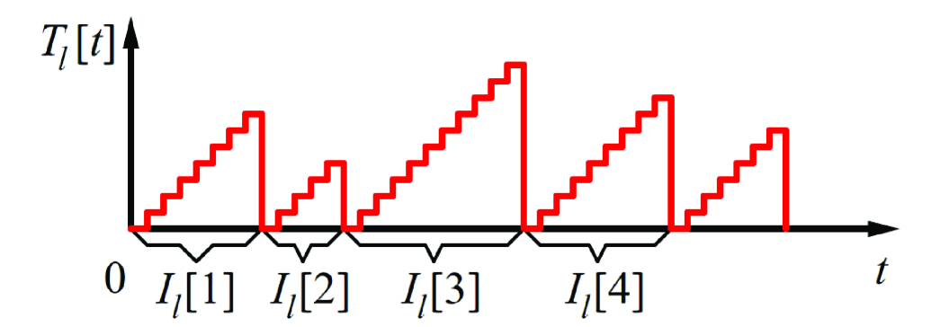
It can be seen from (5) that the evolution of Tl[t]subscript𝑇𝑙delimited-[]𝑡T_{l}[t] differs significantly from that of a traditional queue (also see Fig. 2). In particular, unlike the slowly evolving nature of queue-lengths, the Tl[t]subscript𝑇𝑙delimited-[]𝑡T_{l}[t] is incremented until link l𝑙l receives service at which time it drops to zero. In our design, we will consider policies that not only use queue-lengths to achieve throughput-optimality, but also include TSLS to improve service regularity.

The evolution of Tlsubscript𝑇𝑙T_{l} is tightly related to the inter-service time Ilsubscript𝐼𝑙I_{l}, where Ilsubscript𝐼𝑙I_{l} is the time between two consecutive instances when Tlsubscript𝑇𝑙T_{l} hits zero, as shown in Fig. 2. In fact, we have the following lemma relating the two in steady-state.
Refer to caption
Figure 2: A sample trajectory of Il[m]subscript𝐼𝑙delimited-[]𝑚I_{l}[m] and Tl[t]subscript𝑇𝑙delimited-[]𝑡T_{l}[t], where the curve shows the evolution of Tl[t]subscript𝑇𝑙delimited-[]𝑡T_{l}[t].
Lemma 1

For any policy under which the steady-state distribution of the underlying Markov Chain exists, we have

𝔼[T¯l]=12(1𝔼[I¯l]𝔼[I¯l2]1),𝔼delimited-[]subscript¯𝑇𝑙121𝔼delimited-[]subscript¯𝐼𝑙𝔼delimited-[]superscriptsubscript¯𝐼𝑙21\displaystyle\mathds{E}[\overline{T}_{l}]=\frac{1}{2}\left(\frac{1}{\mathds{E}[\overline{I}_{l}]}\mathds{E}[\overline{I}_{l}^{2}]-1\right), (6)

where T¯lsubscript¯𝑇𝑙\overline{T}_{l} and I¯lsubscript¯𝐼𝑙\overline{I}_{l} denote the steady-state TLSL and inter-service time at link l𝑙l, respectively.

Proof:

The detailed proof is provided in Appendix A. ∎

Lemma 1 reveals the connection between the second moment of the inter-service time I¯lsubscript¯𝐼𝑙\overline{I}_{l} and the mean of TLSL T¯lsubscript¯𝑇𝑙\overline{T}_{l} in steady-state. This can be intuitively seen in Fig. 2, where the area of each “triangle” under the trajectory of Tl[t]subscript𝑇𝑙delimited-[]𝑡T_{l}[t] is roughly 12Il212superscriptsubscript𝐼𝑙2\frac{1}{2}I_{l}^{2}. In this work, we are interested in designing throughput-optimal algorithms that reduce the total weighted-sum222The weighting parameter ρlsubscript𝜌𝑙\rho_{l} is the arrival intensity at link l𝑙l, and indicates that the link with higher load prefers more regular service. Despite this, ρlsubscript𝜌𝑙\rho_{l} is included in the objective function primarily for technical reasons. Noting that the link preference parameter βlsubscript𝛽𝑙\beta_{l} can be any non-negative real number, and thus this weighted form is still general enough. of the normalized second moment of the inter-service time, i.e., l=1Lβlρl𝔼[I¯l2]/(𝔼[I¯l])2superscriptsubscript𝑙1𝐿subscript𝛽𝑙subscript𝜌𝑙𝔼delimited-[]superscriptsubscript¯𝐼𝑙2superscript𝔼delimited-[]subscript¯𝐼𝑙2\sum_{l=1}^{L}\beta_{l}\rho_{l}\mathds{E}[\overline{I}_{l}^{2}]/\left(\mathds{E}[\overline{I}_{l}]\right)^{2}, where μl1/𝔼[I¯l]subscript𝜇𝑙1𝔼delimited-[]subscript¯𝐼𝑙\mu_{l}\triangleq 1/\mathds{E}[\overline{I}_{l}], ρlλl/μlsubscript𝜌𝑙subscript𝜆𝑙subscript𝜇𝑙\rho_{l}\triangleq\lambda_{l}/\mu_{l}, and βl0subscript𝛽𝑙0\beta_{l}\geq 0 is some parameter related to the link. We can set βl>0subscript𝛽𝑙0\beta_{l}>0 if link l𝑙l prefers regular service and βl=0subscript𝛽𝑙0\beta_{l}=0 otherwise.

According to Lemma 1, we have

l=1Lβlρl𝔼[I¯l2](𝔼[I¯l])2=2l=1Lβlλl𝔼[T¯l]+l=1Lβlλl.superscriptsubscript𝑙1𝐿subscript𝛽𝑙subscript𝜌𝑙𝔼delimited-[]superscriptsubscript¯𝐼𝑙2superscript𝔼delimited-[]subscript¯𝐼𝑙22superscriptsubscript𝑙1𝐿subscript𝛽𝑙subscript𝜆𝑙𝔼delimited-[]subscript¯𝑇𝑙superscriptsubscript𝑙1𝐿subscript𝛽𝑙subscript𝜆𝑙\displaystyle\sum_{l=1}^{L}\beta_{l}\rho_{l}\frac{\mathds{E}[\overline{I}_{l}^{2}]}{\left(\mathds{E}[\overline{I}_{l}]\right)^{2}}=2\sum_{l=1}^{L}\beta_{l}\lambda_{l}\mathds{E}[\overline{T}_{l}]+\sum_{l=1}^{L}\beta_{l}\lambda_{l}. (7)

Since l=1Lβlλlsuperscriptsubscript𝑙1𝐿subscript𝛽𝑙subscript𝜆𝑙\sum_{l=1}^{L}\beta_{l}\lambda_{l} only depends on the system parameters, we will use l=1Lβlλl𝔼[T¯l]superscriptsubscript𝑙1𝐿subscript𝛽𝑙subscript𝜆𝑙𝔼delimited-[]subscript¯𝑇𝑙\sum_{l=1}^{L}\beta_{l}\lambda_{l}\mathds{E}[\overline{T}_{l}] as our measure for the service regularity. In this work, we aim to design a scheduling policy that is not only throughput-optimal, but also yields provable good characteristics in the service regularity.

We achieve this dual objective by developing a parametric class of throughput-optimal schedulers (cf. Section III-B) that utilize a combination of queue-lengths and TSLS in its decisions. Our policy is shown to guarantee a ratio (as a function of the system statistics) in its service regularity with respect to a fundamental lower bound (cf. Section IV-A).

III Algorithm design for regular service

In this section, we first discuss the inefficiency of the well-known throughput-optimal Maximum Weight Scheduling (MWS) Algorithm in terms of service regularity. We then propose Regular Service Guarantee policy which can be shown that not only achieves the throughput optimality but also possesses good service regularity performance.

III-A Inefficiency of the MWS Algorithm

In this subsection, we describe a well-known scheduling policy, namely the Maximum Weight Scheduling (MWS) Algorithm and discuss its inefficiency in terms of service regularity performance. We first give the definition of the MWS Algorithm for completeness.

Definition 1 (Maximum Weight Scheduling (MWS) Algorithm)

Under our model, the MWS Algorithm selects a schedule 𝐒(MWS)[t]superscript𝐒MWSdelimited-[]𝑡\mathbf{S}^{(\text{MWS})}[t] with the largest total sum of the product of queue-length and the maximum channel available rate within that schedule, i.e., it chooses

𝐒(MWS)[t]argmax𝐒𝒮l=1LQl[t]Cl[t]Sl[t].superscript𝐒MWSdelimited-[]𝑡subscriptargmax𝐒𝒮superscriptsubscript𝑙1𝐿subscript𝑄𝑙delimited-[]𝑡subscript𝐶𝑙delimited-[]𝑡subscript𝑆𝑙delimited-[]𝑡\displaystyle\mathbf{S}^{(\text{MWS})}[t]\in\operatornamewithlimits{arg\,max}_{\mathbf{S}\in\mathcal{S}}\sum_{l=1}^{L}Q_{l}[t]C_{l}[t]S_{l}[t]. (8)

The MWS Algorithm is known to be throughput-optimal (e.g., [24, 16, 20, 2]), i.e., it stabilizes the network for any arrival rate vector 𝝀𝝀\boldsymbol{\lambda} that strictly lies within the capacity region \mathcal{R}. In our setup, the MWS Algorithm can be expected to have close-to-lower-bound average delay performance (see [5]). It has also been shown to be heavy-traffic optimal (see [22, 3]), i.e., it minimizes the mean steady-state queue-length under heavy-traffic conditions, where the arrival rate vector approaches the boundary of the capacity region from below.

However, despite its throughput optimality and a number of favorable properties on the delay performance, the MWS Algorithm may result in poor performance in terms of service regularity. This can be observed when the MWS Algorithm serves a set of links with heterogeneous arrival statistics in a non-fading single-hop network with uniform link rates.
Refer to caption
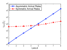
Figure 3: The variance of the inter-service time under the MWS Algorithm for links with different arrival processes. The links with smaller rates or more bursty arrivals suffer from high variance of the inter-service time.

In Fig. 3, the blue line shows a scenario where the lthsuperscript𝑙𝑡l^{th} link has a Bernoulli arrival with rate 2lsuperscript2𝑙2^{-l} for l{1,,8}𝑙18l\in\{1,\dots,8\}. In this case, we observe that the variance of the inter-service time increases exponentially as the arrival rate of the link reduces. The red curve illustrates a different scenario where all 888 links have the same mean arrival rate, but increasing variances (i.e., burstiness) in their arrivals, where we observe that the link with more bursty arrivals suffers from higher variance in its inter-service time.

III-B The Regular Service Guarantee Policy

As discussed above, the MWS Algorithm is throughput-optimal but inefficient in providing regular services. Note that the introduced TLSL counter has a direct impact on service regularity: the smaller the mean TLSL value, the more regular the service. This interesting connection motivates the following parametrized policy which is later revealed to possess the characteristics of throughput optimality and service regularity.


Definition 2 (Regular Service Guarantee (RSG) Algorithm)

In each time slot t𝑡t, select a schedule 𝐒[t]superscript𝐒delimited-[]𝑡\mathbf{S}^{*}[t] such that

𝐒[t]argmax𝐒𝒮l=1L(αlQl[t]+γβlTl[t])Cl[t]Sl,superscript𝐒delimited-[]𝑡subscriptargmax𝐒𝒮superscriptsubscript𝑙1𝐿subscript𝛼𝑙subscript𝑄𝑙delimited-[]𝑡𝛾subscript𝛽𝑙subscript𝑇𝑙delimited-[]𝑡subscript𝐶𝑙delimited-[]𝑡subscript𝑆𝑙\displaystyle\mathbf{S}^{*}[t]\in\operatornamewithlimits{arg\,max}_{\mathbf{S}\in\mathcal{S}}\sum_{l=1}^{L}(\alpha_{l}Q_{l}[t]+\gamma\beta_{l}T_{l}[t])C_{l}[t]S_{l}, (9)

where αl>0subscript𝛼𝑙0\alpha_{l}>0 and γ0𝛾0\gamma\geq 0 are fixed control parameters.


We note that there are two sets of control parameters in the RSG Algorithm333The RSG Algorithm inherits the same complexity issue as the well-known MWS Algorithm. The low complexity or the distributed implementations of the RSG Algorithm are always attractive in practical networks and are left for future research. and they affect different behaviors of the algorithm. Yet, it will be revealed later that none of them affects its throughput optimality. The parameters αlsubscript𝛼𝑙\alpha_{l} are weighing factors for the queue-lengths, where a larger αlsubscript𝛼𝑙\alpha_{l} will result in a smaller average queue-length. The parameter γ𝛾\gamma is a common weighing factor of TSLS for all links. It will be revealed in Section IV-B that the design parameter γ𝛾\gamma can improve the service regularity as it increases. Also note that when γ=0𝛾0\gamma=0, our policy coincides with the MWS Algorithm. When γ>0𝛾0\gamma>0, with the addition of Tl[t]subscript𝑇𝑙delimited-[]𝑡T_{l}[t] terms in the weight of each link, our algorithm operates completely different from the MWS and its approximate algorithms, which, to the best of our knowledge, are the only known policies possessing the throughput-optimality characteristic in general multi-hop network topologies. Despite of this, we can still show that our algorithm is throughput-optimal.

Proposition 1

The RSG Algorithm with any αl>0subscript𝛼𝑙0\alpha_{l}>0 and γ0𝛾0\gamma\geq 0, is throughput-optimal, i.e., for any arrival rate vector 𝛌Int()𝛌Int\boldsymbol{\lambda}\in\text{Int}(\mathcal{R}), the RSG Algorithm stabilizes the system, with

lim supK1Kt=0K1l=1Lαl𝔼[Ql[t]]B(𝜶,𝜷,γ)2ϵ,subscriptlimit-supremum𝐾1𝐾superscriptsubscript𝑡0𝐾1superscriptsubscript𝑙1𝐿subscript𝛼𝑙𝔼delimited-[]subscript𝑄𝑙delimited-[]𝑡𝐵𝜶𝜷𝛾2italic-ϵ\displaystyle\limsup_{K\rightarrow\infty}\frac{1}{K}\sum_{t=0}^{K-1}\sum_{l=1}^{L}\alpha_{l}\mathds{E}[Q_{l}[t]]\leq\frac{B(\boldsymbol{\alpha},\boldsymbol{\beta},\gamma)}{2\epsilon}, (10)

where Int(𝒜)Int𝒜\text{Int}(\mathcal{A}) denotes the interior points of the region 𝒜𝒜\mathcal{A}, B(𝛂,𝛃,γ)4γCmaxl=1Lβl+l=1Lαl𝔼[Al2[t]+Cl2[t]]𝐵𝛂𝛃𝛾4𝛾subscript𝐶superscriptsubscript𝑙1𝐿subscript𝛽𝑙superscriptsubscript𝑙1𝐿subscript𝛼𝑙𝔼delimited-[]superscriptsubscript𝐴𝑙2delimited-[]𝑡superscriptsubscript𝐶𝑙2delimited-[]𝑡B(\boldsymbol{\alpha},\boldsymbol{\beta},\gamma)\triangleq 4\gamma C_{\max}\sum_{l=1}^{L}\beta_{l}+\sum_{l=1}^{L}\alpha_{l}\mathds{E}\left[A_{l}^{2}[t]+C_{l}^{2}[t]\right], ϵitalic-ϵ\epsilon is some positive constant satisfying 𝛌+ϵ𝟏𝛌italic-ϵ1\boldsymbol{\lambda}+\epsilon\mathbf{1}\in\mathcal{R}, and 𝟏1\mathbf{1} is a vector of ones.

Proof:

Consider the Lyapunov function

W(𝐐[t],𝐓[t])l=1LαlQl2[t]+4γCmaxl=1LβlTl[t].𝑊𝐐delimited-[]𝑡𝐓delimited-[]𝑡superscriptsubscript𝑙1𝐿subscript𝛼𝑙superscriptsubscript𝑄𝑙2delimited-[]𝑡4𝛾subscript𝐶superscriptsubscript𝑙1𝐿subscript𝛽𝑙subscript𝑇𝑙delimited-[]𝑡\displaystyle W(\mathbf{Q}[t],\mathbf{T}[t])\triangleq\sum_{l=1}^{L}\alpha_{l}Q_{l}^{2}[t]+4\gamma C_{\max}\sum_{l=1}^{L}\beta_{l}T_{l}[t]. (11)

It is shown in Appendix B that there exists a positive constant ϵ>0italic-ϵ0\epsilon>0 such that

ΔWΔ𝑊absent\displaystyle\Delta W\triangleq 𝔼[W(𝐐[t+1],𝐓[t+1])W(𝐐[t],𝐓[t])|𝐐[t],𝐓[t]]\displaystyle\mathds{E}\left[W(\mathbf{Q}[t+1],\mathbf{T}[t+1])-W(\mathbf{Q}[t],\mathbf{T}[t])\middle|\mathbf{Q}[t],\mathbf{T}[t]\right]
\displaystyle\leq 2ϵl=1LαlQl[t]+B(𝜶,𝜷,γ).2italic-ϵsuperscriptsubscript𝑙1𝐿subscript𝛼𝑙subscript𝑄𝑙delimited-[]𝑡𝐵𝜶𝜷𝛾\displaystyle-2\epsilon\sum_{l=1}^{L}\alpha_{l}Q_{l}[t]+B(\boldsymbol{\alpha},\boldsymbol{\beta},\gamma). (12)

Taking the expectation on the both sides of (III-B) and summing over t=0,1,,K1𝑡01𝐾1t=0,1,...,K-1, we have the desired result. ∎

Proposition 1 establishes the throughput optimality of the RSG Algorithm, thus Ql[t]subscript𝑄𝑙delimited-[]𝑡Q_{l}[t] and Tl[t]subscript𝑇𝑙delimited-[]𝑡T_{l}[t] will converge in distribution to Q¯lsuperscriptsubscript¯𝑄𝑙\overline{Q}_{l}^{*} and T¯lsuperscriptsubscript¯𝑇𝑙\overline{T}_{l}^{*}, which attain the steady-state distribution under our policy. Proposition 1 also gives an upper bound for the expected total queue-length under the steady-state, which increases linearly with the design parameter γ𝛾\gamma. It will be revealed later that γ𝛾\gamma controls the tradeoff between the average total queue-length, and the service regularity performance, especially in the heterogenous networks.

Next, we will show that all moments of steady-state system variables, such as queue-lengths and TLSL, are bounded under the RSG Algorithm, which enables us to analyze the service regularity performance by using the Lyapunov-type approach developed in [3]. In [6], the sufficient condition for all moments of state variables of a Markov Chain to exist in steady state is given as finding a Lyapunov function that satisfies: (1) it has a negative Lyapunov drift when the system variable is large enough; (2) the absolute value of the Lyapunov drift is bounded or has the exponential tail. Yet, the second condition is hard to hold due to the unique evolution of TLSL counters, which have bounded increment but unbounded decrement. We tackle this challenge by properly partitioning the system space.

Proposition 2

For any arrival rate 𝛌Int()𝛌Int\boldsymbol{\lambda}\in\text{Int}(\mathcal{R}), all moments of steady-state queue length and TLSL exist under the RSG Algorithm with any αl>0subscript𝛼𝑙0\alpha_{l}>0 and γ>0𝛾0\gamma>0.

Proof:

We show the boundedness of 𝔼[eη𝐘[t]2]𝔼delimited-[]superscript𝑒𝜂subscriptnorm𝐘delimited-[]𝑡2\mathds{E}\left[e^{\eta\|\mathbf{Y}[t]\|_{2}}\right] for some η>0𝜂0\eta>0 by intelligently partitioning the system space, where 𝐘[t](𝜶𝐐[t],4γCmax𝜷𝐓[t])𝐘delimited-[]𝑡𝜶𝐐delimited-[]𝑡4𝛾subscript𝐶𝜷𝐓delimited-[]𝑡\mathbf{Y}[t]\triangleq\left(\sqrt{\boldsymbol{\alpha}}\mathbf{Q}[t],\sqrt{4\gamma C_{\max}\boldsymbol{\beta}\mathbf{T}[t]}\right), 𝐱𝐱\sqrt{\mathbf{x}} denotes the component-wise square root of the vector 𝐱𝐱\mathbf{x}, and 𝐱𝐲𝐱𝐲\mathbf{xy} denotes the component-wise product of the vectors 𝐱𝐱\mathbf{x} and 𝐲𝐲\mathbf{y}. Please see our technical report [13] for details. ∎

Having established the throughput optimality and the moment existence of the system states of the RSG Algorithm, we are ready to analyze the service regularity performance, i.e., l=1Lβlλl𝔼[T¯l]superscriptsubscript𝑙1𝐿subscript𝛽𝑙subscript𝜆𝑙𝔼delimited-[]subscript¯𝑇𝑙\sum_{l=1}^{L}\beta_{l}\lambda_{l}\mathds{E}[\overline{T}_{l}].

IV Service Regularity Performance Analysis

In this section, we study the service regularity performance of our proposed RSG Algorithm analytically. We first establish a fundamental lower bound on the service regularity for any feasible scheduling algorithm. Then, we derive an upper bound on the service regularity under the RSG Algorithm. These investigations reveal that the service regularity performance of the RSG Algorithm can be guaranteed to remain within a factor of the lower bound, which is expressed as a function of the system statistics and the design parameters, and can be as low as 222 in some special networks. We assume the parameter γ>0𝛾0\gamma>0 throughout this section.

IV-A Lower Bound Analysis

In this subsection, we derive a lower bound based on a Lyapunov drift argument inspired by the technique used in [3]. To study the lower bound of the service regularity by the Lyapunov drift argument, we consider a class of policies, called 𝒫𝒫\mathcal{P}, that not only stabilize the system but also yield the bounded second moment of the steady-state TSLS444We conjecture that the second moment of the steady-state TSLS is bounded as long as the system is stable. Note that our proposed algorithm, as well as the MWS algorithm, falls into this class by Propositions 1 and 2.

Let T¯l(p)superscriptsubscript¯𝑇𝑙𝑝\overline{T}_{l}^{(p)} and S¯l(p)superscriptsubscript¯𝑆𝑙𝑝\overline{S}_{l}^{(p)} be the steady-state TLSL and scheduling variable for link l𝑙l under policy p𝑝p, respectively. The following lemma gives key identities for the first and second moment of the steady-state TSLS, which are useful in deriving a lower bound on the service regularity.

Lemma 2

For any policy p𝒫𝑝𝒫p\in\mathcal{P}, we have

𝔼[l𝐇¯(p)βlλlT¯l(p)]=𝔼delimited-[]subscript𝑙superscript¯𝐇𝑝subscript𝛽𝑙subscript𝜆𝑙superscriptsubscript¯𝑇𝑙𝑝absent\displaystyle\mathds{E}\left[\sum_{l\in\overline{\mathbf{H}}^{(p)}}\beta_{l}\lambda_{l}\overline{T}_{l}^{(p)}\right]= l=1Lβlλl𝔼[l𝐇¯(p)βlλl],superscriptsubscript𝑙1𝐿subscript𝛽𝑙subscript𝜆𝑙𝔼delimited-[]subscript𝑙superscript¯𝐇𝑝subscript𝛽𝑙subscript𝜆𝑙\displaystyle\sum_{l=1}^{L}\beta_{l}\lambda_{l}-\mathds{E}\left[\sum_{l\in\overline{\mathbf{H}}^{(p)}}\beta_{l}\lambda_{l}\right], (13)
2l=1Lβlλl𝔼[T¯l(p)]=2superscriptsubscript𝑙1𝐿subscript𝛽𝑙subscript𝜆𝑙𝔼delimited-[]superscriptsubscript¯𝑇𝑙𝑝absent\displaystyle 2\sum_{l=1}^{L}\beta_{l}\lambda_{l}\mathds{E}\left[\overline{T}_{l}^{(p)}\right]= l=1Lβlλl𝔼[l𝐇¯(p)βlλl]superscriptsubscript𝑙1𝐿subscript𝛽𝑙subscript𝜆𝑙𝔼delimited-[]subscript𝑙superscript¯𝐇𝑝subscript𝛽𝑙subscript𝜆𝑙\displaystyle\sum_{l=1}^{L}\beta_{l}\lambda_{l}-\mathds{E}\left[\sum_{l\in\overline{\mathbf{H}}^{(p)}}\beta_{l}\lambda_{l}\right]
+𝔼[l𝐇¯(p)βlλl(T¯l(p))2],𝔼delimited-[]subscript𝑙superscript¯𝐇𝑝subscript𝛽𝑙subscript𝜆𝑙superscriptsuperscriptsubscript¯𝑇𝑙𝑝2\displaystyle+\mathds{E}\left[\sum_{l\in\overline{\mathbf{H}}^{(p)}}\beta_{l}\lambda_{l}\left(\overline{T}_{l}^{(p)}\right)^{2}\right], (14)

where 𝐇¯(p){l:C¯lS¯l(p)>0}superscript¯𝐇𝑝conditional-set𝑙subscript¯𝐶𝑙superscriptsubscript¯𝑆𝑙𝑝0\overline{\mathbf{H}}^{(p)}\triangleq\{l:\overline{C}_{l}\overline{S}_{l}^{(p)}>0\}, and 𝐂¯=(C¯l)l=1L¯𝐂superscriptsubscriptsubscript¯𝐶𝑙𝑙1𝐿\overline{\mathbf{C}}=(\overline{C}_{l})_{l=1}^{L} has the same probability distribution as 𝐂[t]=(Cl[t])l=1L𝐂delimited-[]𝑡superscriptsubscriptsubscript𝐶𝑙delimited-[]𝑡𝑙1𝐿\mathbf{C}[t]=(C_{l}[t])_{l=1}^{L}.

Proof:

See Appendix C for the proof. ∎

We are ready to give a lower bound on the service regularity for any feasible policy p𝒫𝑝𝒫p\in\mathcal{P}.

Proposition 3

For any policy p𝒫𝑝𝒫p\in\mathcal{P}, we have

l=1Lβlλl𝔼[T¯l(p)]12(l=1Lβlλlmax𝐒𝒮l𝐒βlλl1)l=1Lβlλl.superscriptsubscript𝑙1𝐿subscript𝛽𝑙subscript𝜆𝑙𝔼delimited-[]superscriptsubscript¯𝑇𝑙𝑝12superscriptsubscript𝑙1𝐿subscript𝛽𝑙subscript𝜆𝑙subscript𝐒𝒮subscript𝑙𝐒subscript𝛽𝑙subscript𝜆𝑙1superscriptsubscript𝑙1𝐿subscript𝛽𝑙subscript𝜆𝑙\displaystyle\sum_{l=1}^{L}\beta_{l}\lambda_{l}\mathds{E}\left[\overline{T}_{l}^{(p)}\right]\geq\frac{1}{2}\left(\frac{\sum_{l=1}^{L}\beta_{l}\lambda_{l}}{\max_{\mathbf{S}\in\mathcal{S}}\sum_{l\in\mathbf{S}}\beta_{l}\lambda_{l}}-1\right)\sum_{l=1}^{L}\beta_{l}\lambda_{l}.
Proof:

In the rest of proof, we will omit superscript p𝑝p for conciseness. For any sample path, by Cauchy-Schwarz inequality, we have

(l𝐇¯βlλlT¯l)2=superscriptsubscript𝑙¯𝐇subscript𝛽𝑙subscript𝜆𝑙subscript¯𝑇𝑙2absent\displaystyle\left(\sum_{l\in\overline{\mathbf{H}}}\beta_{l}\lambda_{l}\overline{T}_{l}\right)^{2}= (l𝐇¯βlλlβlλlT¯l)2superscriptsubscript𝑙¯𝐇subscript𝛽𝑙subscript𝜆𝑙subscript𝛽𝑙subscript𝜆𝑙subscript¯𝑇𝑙2\displaystyle\left(\sum_{l\in\overline{\mathbf{H}}}\sqrt{\beta_{l}\lambda_{l}}\cdot\sqrt{\beta_{l}\lambda_{l}}\overline{T}_{l}\right)^{2}
\displaystyle\leq (l𝐇¯βlλl)l𝐇¯βlλlT¯l2,subscript𝑙¯𝐇subscript𝛽𝑙subscript𝜆𝑙subscript𝑙¯𝐇subscript𝛽𝑙subscript𝜆𝑙superscriptsubscript¯𝑇𝑙2\displaystyle\left(\sum_{l\in\overline{\mathbf{H}}}\beta_{l}\lambda_{l}\right)\sum_{l\in\overline{\mathbf{H}}}\beta_{l}\lambda_{l}\overline{T}_{l}^{2}, (15)

where we recall that 𝐇¯{l:C¯lS¯l>0}¯𝐇conditional-set𝑙subscript¯𝐶𝑙subscript¯𝑆𝑙0\mathbf{\overline{H}}\triangleq\{l:\overline{C}_{l}\overline{S}_{l}>0\}. This implies

l𝐇¯βlλlT¯l2(l𝐇¯βlλlT¯l)2l𝐇¯βlλl.subscript𝑙¯𝐇subscript𝛽𝑙subscript𝜆𝑙superscriptsubscript¯𝑇𝑙2superscriptsubscript𝑙¯𝐇subscript𝛽𝑙subscript𝜆𝑙subscript¯𝑇𝑙2subscript𝑙¯𝐇subscript𝛽𝑙subscript𝜆𝑙\displaystyle\sum_{l\in\overline{\mathbf{H}}}\beta_{l}\lambda_{l}\overline{T}_{l}^{2}\geq\frac{\left(\sum_{l\in\overline{\mathbf{H}}}\beta_{l}\lambda_{l}\overline{T}_{l}\right)^{2}}{\sum_{l\in\overline{\mathbf{H}}}\beta_{l}\lambda_{l}}. (16)

Hence, we have

𝔼[l𝐇¯βlλlT¯l2]𝔼delimited-[]subscript𝑙¯𝐇subscript𝛽𝑙subscript𝜆𝑙superscriptsubscript¯𝑇𝑙2absent\displaystyle\mathds{E}\left[\sum_{l\in\overline{\mathbf{H}}}\beta_{l}\lambda_{l}\overline{T}_{l}^{2}\right]\geq 𝔼[(l𝐇¯βlλlT¯l)2l𝐇¯βlλl]𝔼delimited-[]superscriptsubscript𝑙¯𝐇subscript𝛽𝑙subscript𝜆𝑙subscript¯𝑇𝑙2subscript𝑙¯𝐇subscript𝛽𝑙subscript𝜆𝑙\displaystyle\mathds{E}\left[\frac{\left(\sum_{l\in\overline{\mathbf{H}}}\beta_{l}\lambda_{l}\overline{T}_{l}\right)^{2}}{\sum_{l\in\overline{\mathbf{H}}}\beta_{l}\lambda_{l}}\right]
(a)superscript𝑎\displaystyle\stackrel{{\scriptstyle(a)}}{{\geq}} (𝔼[l𝐇¯βlλlT¯l])2𝔼[l𝐇¯βlλl]superscript𝔼delimited-[]subscript𝑙¯𝐇subscript𝛽𝑙subscript𝜆𝑙subscript¯𝑇𝑙2𝔼delimited-[]subscript𝑙¯𝐇subscript𝛽𝑙subscript𝜆𝑙\displaystyle\frac{\left(\mathds{E}\left[\sum_{l\in\overline{\mathbf{H}}}\beta_{l}\lambda_{l}\overline{T}_{l}\right]\right)^{2}}{\mathds{E}\left[\sum_{l\in\overline{\mathbf{H}}}\beta_{l}\lambda_{l}\right]}
=(b)superscript𝑏\displaystyle\stackrel{{\scriptstyle(b)}}{{=}} (l=1Lβlλl𝔼[l𝐇¯βlλl])2𝔼[l𝐇¯βlλl],superscriptsuperscriptsubscript𝑙1𝐿subscript𝛽𝑙subscript𝜆𝑙𝔼delimited-[]subscript𝑙¯𝐇subscript𝛽𝑙subscript𝜆𝑙2𝔼delimited-[]subscript𝑙¯𝐇subscript𝛽𝑙subscript𝜆𝑙\displaystyle\frac{\left(\sum_{l=1}^{L}\beta_{l}\lambda_{l}-\mathds{E}\left[\sum_{l\in\overline{\mathbf{H}}}\beta_{l}\lambda_{l}\right]\right)^{2}}{\mathds{E}\left[\sum_{l\in\overline{\mathbf{H}}}\beta_{l}\lambda_{l}\right]}, (17)

where the step (a)𝑎(a) uses the fact that f(x,y)=x2y𝑓𝑥𝑦superscript𝑥2𝑦f(x,y)=\frac{x^{2}}{y} is convex and Jensen’s inequality for a multi-variable function; step (b)𝑏(b) follows from (13). By substituting (IV-A) into (14), we have

l=1Lβlλl𝔼[T¯l]12(l=1Lβlλl𝔼[l𝐇¯βlλl]1)l=1Lβlλl.superscriptsubscript𝑙1𝐿subscript𝛽𝑙subscript𝜆𝑙𝔼delimited-[]subscript¯𝑇𝑙12superscriptsubscript𝑙1𝐿subscript𝛽𝑙subscript𝜆𝑙𝔼delimited-[]subscript𝑙¯𝐇subscript𝛽𝑙subscript𝜆𝑙1superscriptsubscript𝑙1𝐿subscript𝛽𝑙subscript𝜆𝑙\displaystyle\sum_{l=1}^{L}\beta_{l}\lambda_{l}\mathds{E}\left[\overline{T}_{l}\right]\geq\frac{1}{2}\left(\frac{\sum_{l=1}^{L}\beta_{l}\lambda_{l}}{\mathds{E}\left[\sum_{l\in\overline{\mathbf{H}}}\beta_{l}\lambda_{l}\right]}-1\right)\sum_{l=1}^{L}\beta_{l}\lambda_{l}. (18)

Note that

𝔼[l𝐇¯βlλl]=𝔼[l=1Lβlλl𝟙{C¯lS¯l>0}]𝔼delimited-[]subscript𝑙¯𝐇subscript𝛽𝑙subscript𝜆𝑙𝔼delimited-[]superscriptsubscript𝑙1𝐿subscript𝛽𝑙subscript𝜆𝑙subscript1subscript¯𝐶𝑙subscript¯𝑆𝑙0\displaystyle\mathds{E}\left[\sum_{l\in\overline{\mathbf{H}}}\beta_{l}\lambda_{l}\right]=\mathds{E}\left[\sum_{l=1}^{L}\beta_{l}\lambda_{l}\mathds{1}_{\{\overline{C}_{l}\overline{S}_{l}>0\}}\right]
=\displaystyle= l=1LβlλlPr{C¯lS¯l>0}superscriptsubscript𝑙1𝐿subscript𝛽𝑙subscript𝜆𝑙Prsubscript¯𝐶𝑙subscript¯𝑆𝑙0\displaystyle\sum_{l=1}^{L}\beta_{l}\lambda_{l}\Pr\{\overline{C}_{l}\overline{S}_{l}>0\}
\displaystyle\leq l=1LβlλlPr{S¯l=1}max𝐒𝒮l𝐒βlλl.superscriptsubscript𝑙1𝐿subscript𝛽𝑙subscript𝜆𝑙Prsubscript¯𝑆𝑙1subscript𝐒𝒮subscript𝑙𝐒subscript𝛽𝑙subscript𝜆𝑙\displaystyle\sum_{l=1}^{L}\beta_{l}\lambda_{l}\Pr\{\overline{S}_{l}=1\}\leq\max_{\mathbf{S}\in\mathcal{S}}\sum_{l\in\mathbf{S}}\beta_{l}\lambda_{l}. (19)

By substituting (IV-A) into (18), we have the desired result. ∎

Consider a single-hop non-fading network, where only one link is scheduled in each time slot. Let βl=βsubscript𝛽𝑙𝛽\beta_{l}=\beta and λl=λsubscript𝜆𝑙𝜆\lambda_{l}=\lambda for each link l𝑙l. Then, the lower bound becomes

l=1L𝔼[T¯l(p)]12L(L1).superscriptsubscript𝑙1𝐿𝔼delimited-[]superscriptsubscript¯𝑇𝑙𝑝12𝐿𝐿1\displaystyle\sum_{l=1}^{L}\mathds{E}\left[\overline{T}_{l}^{(p)}\right]\geq\frac{1}{2}L(L-1). (20)

This lower bound can be achieved by the Round-Robin (RR) policy, which serves each link periodically. Thus, in the steady-state, the TSLS vector under the RR policy is a permutation of {0,1,2,,L1}012𝐿1\{0,1,2,...,L-1\} and thus l=1L𝔼[T¯l(RR)]=12L(L1).superscriptsubscript𝑙1𝐿𝔼delimited-[]superscriptsubscript¯𝑇𝑙RR12𝐿𝐿1\sum_{l=1}^{L}\mathds{E}\left[\overline{T}_{l}^{(\text{RR})}\right]=\frac{1}{2}L(L-1).

Yet, we would like to point out that the RR policy is not throughput-optimal. Thus, for an arrival rate vector 𝝀𝝀\boldsymbol{\lambda} that cannot be supported by the RR policy, we do not expect a throughput-optimal policy to approach the above lower bound when serving it. However, for the arrival rate vectors that can be supported by the RR policy, we shall see in our numerical results that the performance of our policy can approach this lower bound when we increase the scaling parameter γ𝛾\gamma.

IV-B Upper Bound Analysis

In this subsection, we obtain an upper bound on the service regularity under the RSG Algorithm. Let Q¯lsuperscriptsubscript¯𝑄𝑙\overline{Q}_{l}^{*}, S¯lsuperscriptsubscript¯𝑆𝑙\overline{S}_{l}^{*} and T¯lsuperscriptsubscript¯𝑇𝑙\overline{T}_{l}^{*} be the steady-state queue-length, scheduling variable and TSLS for link l𝑙l under the RSG Algorithm, respectively.

Proposition 4

For the RSG Algorithm, we have

l=1Lβlλl𝔼[T¯l]superscriptsubscript𝑙1𝐿subscript𝛽𝑙subscript𝜆𝑙𝔼delimited-[]superscriptsubscript¯𝑇𝑙absent\displaystyle\sum_{l=1}^{L}\beta_{l}\lambda_{l}\mathds{E}\left[\overline{T}_{l}^{*}\right]\leq Cmax1+ϵ(l=1Lβl𝔼[l𝐇¯βl])subscript𝐶1italic-ϵsuperscriptsubscript𝑙1𝐿subscript𝛽𝑙𝔼delimited-[]subscript𝑙superscript¯𝐇subscript𝛽𝑙\displaystyle\frac{C_{\max}}{1+\epsilon}\left(\sum_{l=1}^{L}\beta_{l}-\mathds{E}\left[\sum_{l\in\overline{\mathbf{H}}^{*}}\beta_{l}\right]\right)
+12γ(1+ϵ)l=1Lαl𝔼[A¯l2+C¯l2],12𝛾1italic-ϵsuperscriptsubscript𝑙1𝐿subscript𝛼𝑙𝔼delimited-[]superscriptsubscript¯𝐴𝑙2superscriptsubscript¯𝐶𝑙2\displaystyle+\frac{1}{2\gamma(1+\epsilon)}\sum_{l=1}^{L}\alpha_{l}\mathds{E}\left[\overline{A}_{l}^{2}+\overline{C}_{l}^{2}\right], (21)

where ϵ>0italic-ϵ0\epsilon>0 satisfies 𝛌(1+ϵ)𝛌1italic-ϵ\boldsymbol{\lambda}(1+\epsilon)\in\mathcal{R}, 𝐇¯{l:C¯lS¯l>0}superscript¯𝐇conditional-set𝑙subscript¯𝐶𝑙superscriptsubscript¯𝑆𝑙0\overline{\mathbf{H}}^{*}\triangleq\{l:\overline{C}_{l}\overline{S}_{l}^{*}>0\}, and 𝐀¯=(A¯l)l=1L¯𝐀superscriptsubscriptsubscript¯𝐴𝑙𝑙1𝐿\overline{\mathbf{A}}=(\overline{A}_{l})_{l=1}^{L} has the same distribution as 𝐀[t]=(Al[t])l=1L𝐀delimited-[]𝑡superscriptsubscriptsubscript𝐴𝑙delimited-[]𝑡𝑙1𝐿\mathbf{A}[t]=(A_{l}[t])_{l=1}^{L}.

Proof:

See Appendix D for the details. ∎

Note that the second term of the right hand side of (4) captures various random effects in the network: the burstiness of the arrival processes and the channel variations. Under our policy these effects diminish as the scaling factor γ𝛾\gamma goes to infinity. Hence, together with Proposition 1, Proposition 4 reveals a tradeoff: when increasing γ𝛾\gamma, the upper bound on the total queue-length increases linearly with γ𝛾\gamma, but the upper bound for the service regularity decreases.

Consider the single-hop non-fading network as in Section IV-A. Let βl=βsubscript𝛽𝑙𝛽\beta_{l}=\beta and λl=λ=1L(1+ϵ)subscript𝜆𝑙𝜆1𝐿1italic-ϵ\lambda_{l}=\lambda=\frac{1}{L(1+\epsilon)} for each link l𝑙l. Then, as γ𝛾\gamma goes to infinity, (4) becomes

l=1L𝔼[T¯l]L(L1),superscriptsubscript𝑙1𝐿𝔼delimited-[]superscriptsubscript¯𝑇𝑙𝐿𝐿1\displaystyle\sum_{l=1}^{L}\mathds{E}\left[\overline{T}_{l}^{*}\right]\leq L(L-1), (22)

which is always within twice the value of the lower bound (20). In the more general case, the upper bound converges to a constant that is determined by the system statistics and design parameters as γ𝛾\gamma goes to infinity. Moreover, we shall see in the numerical results presented in Section V-B that as γ𝛾\gamma increases, the service regularity performance under the RSG Algorithm actually converges to the lower bound (20) in the single-hop non-fading network with the symmetric parameters.
Refer to caption
(a) Single-hop non-fading network
Refer to caption
(b) Single-hop fading network
Refer to caption
(c) 3×3333\times 3 switch
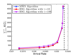
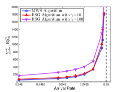
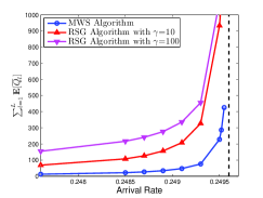
Figure 4: The throughput performance of the RSG Algorithm
Refer to caption
(a) Single-hop non-fading network
Refer to caption
(b) Single-hop fading network
Refer to caption
(c) 3×3333\times 3 switch
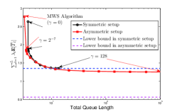
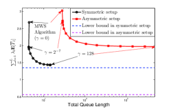
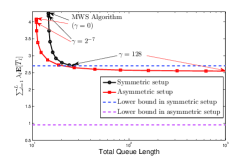
Figure 5: Trade-off between mean queue length and the service regularity

V Numerical Results

In this section, we provide simulation results for our proposed RSG Algorithm and compare its performance to the MWS Algorithm and bounds. In addition to investigating the throughput (cf. Section V-A) and service regularity (cf. Section V-B) performances of our policy in both single-hop network with L=4𝐿4L=4 links and 3×3333\times 3 switch, we also look at the behavior of the RSG Algorithm as well as the potential benefit of the service regularity (cf. Section V-C). In the first two simulations, we assume Bernoulli arrivals to each link and αl=βl=1subscript𝛼𝑙subscript𝛽𝑙1\alpha_{l}=\beta_{l}=1 for each link l𝑙l.

V-A Throughput Performance

In this subsection, we illustrate the throughput performance of the RSG Algorithm in three different network setups with symmetric arrivals: (i) single-hop non-fading network, (ii) single-hop network with symmetric ON-OFF fading channels with probability q=0.8𝑞0.8q=0.8 that the channel is available, and (iii) 3×3333\times 3 switch. The achievable rate regions for these three networks, respectively, are

Λ1subscriptΛ1absent\displaystyle\Lambda_{1}\triangleq {𝝀=(λl)l=14:λ1=λ2==λ4<14},conditional-set𝝀superscriptsubscriptsubscript𝜆𝑙𝑙14subscript𝜆1subscript𝜆2subscript𝜆414\displaystyle\left\{\boldsymbol{\lambda}=(\lambda_{l})_{l=1}^{4}:\lambda_{1}=\lambda_{2}=...=\lambda_{4}<\frac{1}{4}\right\},
Λ2subscriptΛ2absent\displaystyle\Lambda_{2}\triangleq {𝝀=(λl)l=14:λ1=λ2==λ4<1(1q)44},conditional-set𝝀superscriptsubscriptsubscript𝜆𝑙𝑙14subscript𝜆1subscript𝜆2subscript𝜆41superscript1𝑞44\displaystyle\left\{\boldsymbol{\lambda}=(\lambda_{l})_{l=1}^{4}:\lambda_{1}=\lambda_{2}=...=\lambda_{4}<\frac{1-(1-q)^{4}}{4}\right\},
Λ3subscriptΛ3absent\displaystyle\Lambda_{3}\triangleq {𝝀=(λl)l=19:λ1=λ2==λ9<13}.conditional-set𝝀superscriptsubscriptsubscript𝜆𝑙𝑙19subscript𝜆1subscript𝜆2subscript𝜆913\displaystyle\left\{\boldsymbol{\lambda}=(\lambda_{l})_{l=1}^{9}:\lambda_{1}=\lambda_{2}=...=\lambda_{9}<\frac{1}{3}\right\}.

In Fig. 4, we compare the total mean queue-length under the MWS Algorithm, as well as the RSG Algorithm with different γ𝛾\gamma values. It can be observed in Fig. 4 that the RSG Algorithm can stabilize the system in the above network setups. It also can be seen that the total mean queue-length of the RSG Algorithm increases with the parameter γ𝛾\gamma. This is expected since as γ𝛾\gamma increases, it becomes more likely for the RSG Algorithm to choose a queue with less packet to serve, potentially wasting some service while improving the service regularity, as we shall see next.

V-B Service Regularity Performance

In this subsection, we investigate the service regularity performance of our RSG Algorithm, as well as illustrate the tradeoff between the total mean queue-length and the service regularity. We present our results in three different networks: single-hop non-fading network, single-hop fading network and 3×3333\times 3 switch. In both single-hop nonfading and fading networks, we consider the symmetric setup with the arrival rate vector 𝝀[0.225,0.225,0.225,0.225]𝝀0.2250.2250.2250.225\boldsymbol{\lambda}\triangleq[0.225,0.225,0.225,0.225], and the asymmetric setup with the arrival rate vector 𝝀[0.4,0.3,0.15,0.05]𝝀0.40.30.150.05\boldsymbol{\lambda}\triangleq[0.4,0.3,0.15,0.05]. For a single-hop ON-OFF fading network, the probability vectors that the channels are available are 𝐪=[0.8,0.8,0.8,0.8]𝐪0.80.80.80.8\mathbf{q}=[0.8,0.8,0.8,0.8] in symmetric setup and 𝐪=[0.6,0.5,0.4,0.3]𝐪0.60.50.40.3\mathbf{q}=[0.6,0.5,0.4,0.3] in asymmetric setup. For a 3×3333\times 3 switch, we consider the symmetric setup with the arrival rate vector 𝝀[0.3,0.3,0.3;0.3,0.3,0.3;0.3,0.3,0.3]𝝀0.30.30.30.30.30.30.30.30.3\boldsymbol{\lambda}\triangleq[0.3,0.3,0.3;0.3,0.3,0.3;0.3,0.3,0.3] and the asymmetric setup with the arrival rate vector 𝝀[0.5,0.3,0.1;0.2,0.4,0.3;0.1,0.2,0.5]𝝀0.50.30.10.20.40.30.10.20.5\boldsymbol{\lambda}\triangleq[0.5,0.3,0.1;0.2,0.4,0.3;0.1,0.2,0.5]. In all simulations, we choose the scaling parameter γ𝛾\gamma to be the powers of 2, ranging from 27superscript272^{-7} to 27superscript272^{7}.

Fig. 5 shows the relationship between the total mean queue-length and the service regularity in different network setups. The tradeoff between the service regularity and the total mean queue-length can be clearly seen: as γ𝛾\gamma increases, the service regularity improves while the total mean queue-length also increases. It can be observed that the simulated values converge to the fundamental lower bound in non-fading networks with symmetric setup (Figs 5(a) and (c)), while they stay away from the lower bound in asymmetric setups. This motivates us to refine the lower bound analysis in asymmetric setups, which is left for future investigation. Here, it is worth mentioning that even with very small γ𝛾\gamma values (e.g., 26superscript262^{-6}), our RSG Algorithm significantly improves the service regularity, while introducing negligible increase in the total mean queue-length.
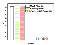
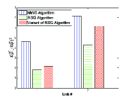
Refer to caption
(a) Mean unused service
Refer to caption
(b) Service regularity performance
Refer to caption
(c) Mean queue length
Refer to caption
(d) Standard deviation of queue length
Figure 6: Performance comparison between the RSG Algorithm and the MWS Algorithm

V-C Benefit of the Service Regularity

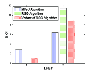
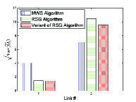
In this subsection, we study various performance metrics (such as mean unused service, service regularity, mean queue-length and variance of queue-length) among links to illustrate the behavior of the RSG Algorithm as well as the benefit of the service regularity. To that end, we consider a single-hop non-fading network with two links. Each link can serve 444 packets in each time slot if scheduled. There is always 111 packet arriving at the first link in each time slot, while the number of packets arriving at the second link is either 2K2𝐾2K with probability 1/K1𝐾1/K or 00, where K𝐾K is a natural number. We compare the performance between the MWS Algorithm, the RSG Algorithm and the variant of the RSG Algorithm whose TSLS counter increases only when the link does not receive service and the link queue-length is non-zero. In both RSG Algorithm and its variant, we set β1=1,β2=0,γ=10formulae-sequencesubscript𝛽11formulae-sequencesubscript𝛽20𝛾10\beta_{1}=1,\beta_{2}=0,\gamma=10, i.e., we assume that the first link prefers the regular service while the second link does not have such a requirement. In the following simulations, we set K=5𝐾5K=5.

From Fig. 6a, we observe that compared to the MWS Algorithm, under the RSG Algorithm, the mean unused service in the first link slightly increases, while in the second it slightly decreases. This is expected since the TSLS counter increases even when the queue-length is non-zero. Yet, the total amount of mean unused service under the RSG Algorithm remains the same as that under the MWS Algorithm. For the variant of the RSG Algorithm, the mean unused service for each individual link almost does not change.

From Fig. 6b, we can see that both the RSG Algorithm and its variant improve the service regularity compared to the MWS Algorithm. Also, the RSG Algorithm yields the better service regularity performance than its variant. This is because the TSLS counter under the variant of the RSG Algorithm is not as aggressive as that under the original RSG Algorithm. As can be seen in Fig. 6c and Fig. 6d, providing more regular service is extremely beneficial for the link with constant arrivals since it leads to the smaller mean and variance of delay that each packet experiences in that link.

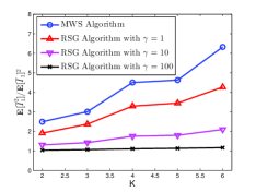
Next, we would like to reveal the relationship between the service regularity of the first link with constant arrivals and the burstiness of arrivals at the second link that is reflected by the parameter K𝐾K. The larger the K𝐾K, the more bursty the arrivals at the second link. Fig. 7 shows the impact of the bursty arrivals on the service regularity of the link with the constant arrival under both MWS and RSG Algorithms. We can observe from Fig. 7 that the service regularity of the first link under the MWS Algorithm degrades much faster than that under the RSG Algorithm as the the burstiness of the second link increases. Also, as γ𝛾\gamma increases, under the RSG Algorithm, the service regularity of the first link improves significantly, and it is almost independent of the burstiness of the second link when γ=100𝛾100\gamma=100.

Refer to caption
Figure 7: The impact of the bursty arrivals on the service regularity of the constant flow

VI Conclusion

In this work, we investigated the problem of designing a scheduling policy that is both throughput-optimal and possesses favorable service regularity characteristics. We introduced a new parameter of time-since-last-service, and proposed a novel scheduling policy that combines this parameter with the queue-lengths in its weight. After establishing the throughput optimality of our policy, we showed that it also has provable service regularity performance. In particular, the service regularity of our policy can be guaranteed to remain within a factor distance of a fundamental lower bound for any feasible scheduling policy. We explicitly expressed this factor as a function of the system statistics and the design parameters. We performed extensive numerical studies to illustrate the significant gains achieved by our policy over the traditional queue-length-based policies. Our results show the significance of utilizing the time-since-last-service in improving the service regularity performance of throughput-optimal policies.

Appendix A Proof of Lemma 1

Without loss of generality, assume that link l𝑙l is served at time 00. For any positive integer M𝑀M, there exists an m𝑚m such that

Il[1]++Il[m]subscript𝐼𝑙delimited-[]1subscript𝐼𝑙delimited-[]𝑚\displaystyle I_{l}[1]+\dots+I_{l}[m] \displaystyle\leq M,𝑀\displaystyle M,
Il[1]++Il[m]+Il[m+1]subscript𝐼𝑙delimited-[]1subscript𝐼𝑙delimited-[]𝑚subscript𝐼𝑙delimited-[]𝑚1\displaystyle I_{l}[1]+\dots+I_{l}[m]+I_{l}[m+1] >\displaystyle> M.𝑀\displaystyle M.

We can write

1Mt=1MTl[t]1𝑀superscriptsubscript𝑡1𝑀subscript𝑇𝑙delimited-[]𝑡\displaystyle\frac{1}{M}\sum_{t=1}^{M}T_{l}[t] =\displaystyle= 1M(t=1Il[1]Tl[t]+t=Il[1]+1Il[1]+Il[2]Tl[t]+\displaystyle\frac{1}{M}\Bigg{(}\sum_{t=1}^{I_{l}[1]}T_{l}[t]+\sum_{t=I_{l}[1]+1}^{I_{l}[1]+I_{l}[2]}T_{l}[t]+\dots (23)
+t=Il[1]++Il[m]+1MTl[t]).\displaystyle+\sum_{t=I_{l}[1]+\dots+I_{l}[m]+1}^{M}T_{l}[t]\Bigg{)}.

We observe the following fact: assume link l𝑙l receives its (m1)thsuperscript𝑚1𝑡(m-1)^{th} and mthsuperscript𝑚𝑡m^{th} service at time slot t1subscript𝑡1t_{1} and t2subscript𝑡2t_{2}, respectively, where t2>t1subscript𝑡2subscript𝑡1t_{2}>t_{1}. Then, by definition, Il[m]=t2t1subscript𝐼𝑙delimited-[]𝑚subscript𝑡2subscript𝑡1I_{l}[m]=t_{2}-t_{1}, Tl[t1+1]=0subscript𝑇𝑙delimited-[]subscript𝑡110T_{l}[t_{1}+1]=0 and Tl[t2]=t2t11=Il[m]1subscript𝑇𝑙delimited-[]subscript𝑡2subscript𝑡2subscript𝑡11subscript𝐼𝑙delimited-[]𝑚1T_{l}[t_{2}]=t_{2}-t_{1}-1=I_{l}[m]-1. Using this fact, we know the kthsuperscript𝑘𝑡k^{th} summation on the right hand side of (23) gives 12(Il[k](Il[k]1))12subscript𝐼𝑙delimited-[]𝑘subscript𝐼𝑙delimited-[]𝑘1\frac{1}{2}(I_{l}[k](I_{l}[k]-1)), except for the last one. Thus we have:

1Mt=1MTl[t]1𝑀superscriptsubscript𝑡1𝑀subscript𝑇𝑙delimited-[]𝑡\displaystyle\frac{1}{M}\sum_{t=1}^{M}T_{l}[t] \displaystyle\geq 1Mk=1mIl[k](Il[k]1)2,1𝑀superscriptsubscript𝑘1𝑚subscript𝐼𝑙delimited-[]𝑘subscript𝐼𝑙delimited-[]𝑘12\displaystyle\frac{1}{M}\sum_{k=1}^{m}\frac{I_{l}[k](I_{l}[k]-1)}{2}, (24)
1Mt=1MTl[t]1𝑀superscriptsubscript𝑡1𝑀subscript𝑇𝑙delimited-[]𝑡\displaystyle\frac{1}{M}\sum_{t=1}^{M}T_{l}[t] \displaystyle\leq 1Mk=1m+1Il[k](Il[k]1)2.1𝑀superscriptsubscript𝑘1𝑚1subscript𝐼𝑙delimited-[]𝑘subscript𝐼𝑙delimited-[]𝑘12\displaystyle\frac{1}{M}\sum_{k=1}^{m+1}\frac{I_{l}[k](I_{l}[k]-1)}{2}. (25)

By the definition of m𝑚m and the fact that 𝔼[I¯l]<𝔼delimited-[]subscript¯𝐼𝑙\mathds{E}[\overline{I}_{l}]<\infty when each link is served with strictly positive probability, we know that m𝑚m\rightarrow\infty when M𝑀M\rightarrow\infty. Since the policy considered in this paper is Markovian, we have

limM1Mt=1MTl[t]=𝔼[T¯l],subscript𝑀1𝑀superscriptsubscript𝑡1𝑀subscript𝑇𝑙delimited-[]𝑡𝔼delimited-[]subscript¯𝑇𝑙\displaystyle\lim_{M\rightarrow\infty}\frac{1}{M}\sum_{t=1}^{M}T_{l}[t]=\mathds{E}[\overline{T}_{l}],
limm1mk=1mIl[k]=𝔼[I¯l],subscript𝑚1𝑚superscriptsubscript𝑘1𝑚subscript𝐼𝑙delimited-[]𝑘𝔼delimited-[]subscript¯𝐼𝑙\displaystyle\lim_{m\rightarrow\infty}\frac{1}{m}\sum_{k=1}^{m}I_{l}[k]=\mathds{E}[\overline{I}_{l}],
limm1mk=1mIl2[k]=𝔼[I¯l2].subscript𝑚1𝑚superscriptsubscript𝑘1𝑚superscriptsubscript𝐼𝑙2delimited-[]𝑘𝔼delimited-[]superscriptsubscript¯𝐼𝑙2\displaystyle\lim_{m\rightarrow\infty}\frac{1}{m}\sum_{k=1}^{m}I_{l}^{2}[k]=\mathds{E}[\overline{I}_{l}^{2}].

Note that

1mk=1mIl[k]Mmm+1m1m+1k=1m+1Il[k],1𝑚superscriptsubscript𝑘1𝑚subscript𝐼𝑙delimited-[]𝑘𝑀𝑚𝑚1𝑚1𝑚1superscriptsubscript𝑘1𝑚1subscript𝐼𝑙delimited-[]𝑘\displaystyle\frac{1}{m}\sum_{k=1}^{m}I_{l}[k]\leq\frac{M}{m}\leq\frac{m+1}{m}\frac{1}{m+1}\sum_{k=1}^{m+1}I_{l}[k],

which implies limMMm=𝔼[I¯l].subscript𝑀𝑀𝑚𝔼delimited-[]subscript¯𝐼𝑙\lim_{M\rightarrow\infty}\frac{M}{m}=\mathds{E}[\overline{I}_{l}].

By taking limit on (24) and (25) as M𝑀M\rightarrow\infty, we have

limMmM1mk=1mIl[k](Il[k]1)2subscript𝑀𝑚𝑀1𝑚superscriptsubscript𝑘1𝑚subscript𝐼𝑙delimited-[]𝑘subscript𝐼𝑙delimited-[]𝑘12\displaystyle\lim_{M\rightarrow\infty}\frac{m}{M}\frac{1}{m}\sum_{k=1}^{m}\frac{I_{l}[k](I_{l}[k]-1)}{2}
\displaystyle\leq limM1Mt=1MTl[t]subscript𝑀1𝑀superscriptsubscript𝑡1𝑀subscript𝑇𝑙delimited-[]𝑡\displaystyle\lim_{M\rightarrow\infty}\frac{1}{M}\sum_{t=1}^{M}T_{l}[t]
\displaystyle\leq limMm+1M1m+1k=1m+1Il[k](Il[k]1)2,subscript𝑀𝑚1𝑀1𝑚1superscriptsubscript𝑘1𝑚1subscript𝐼𝑙delimited-[]𝑘subscript𝐼𝑙delimited-[]𝑘12\displaystyle\lim_{M\rightarrow\infty}\frac{m+1}{M}\frac{1}{m+1}\sum_{k=1}^{m+1}\frac{I_{l}[k](I_{l}[k]-1)}{2},

and thus we have the desired result.

Appendix B Proof of inequality (III-B)

ΔWΔ𝑊absent\displaystyle\Delta W\triangleq 𝔼[W(𝐐[t+1],𝐓[t+1])W(𝐐[t],𝐓[t])|𝐐[t],𝐓[t]]\displaystyle\mathds{E}\left[W(\mathbf{Q}[t+1],\mathbf{T}[t+1])-W(\mathbf{Q}[t],\mathbf{T}[t])\middle|\mathbf{Q}[t],\mathbf{T}[t]\right]
=\displaystyle= 𝔼[l=1LαlQl2[t+1]+4γCmaxl=1LβlTl[t+1]\displaystyle\mathds{E}\Bigg{[}\sum_{l=1}^{L}\alpha_{l}Q_{l}^{2}[t+1]+4\gamma C_{\max}\sum_{l=1}^{L}\beta_{l}T_{l}[t+1]
l=1LαlQl2[t]4γCmaxl=1LβlTl[t]|𝐐[t],𝐓[t]]\displaystyle-\sum_{l=1}^{L}\alpha_{l}Q_{l}^{2}[t]-4\gamma C_{\max}\sum_{l=1}^{L}\beta_{l}T_{l}[t]\Bigg{|}\mathbf{Q}[t],\mathbf{T}[t]\Bigg{]}
\displaystyle\leq l=1Lαl𝔼[(Ql[t]+Al[t]Cl[t]Sl[t])2Ql2[t]|𝐐[t],𝐓[t]]\displaystyle\sum_{l=1}^{L}\alpha_{l}\mathds{E}\left[(Q_{l}[t]+A_{l}[t]-C_{l}[t]S_{l}^{*}[t])^{2}-Q_{l}^{2}[t]\middle|\mathbf{Q}[t],\mathbf{T}[t]\right]
+4γCmax𝔼[l=1LβlTl[t+1]l=1LβlTl[t]|𝐐[t],𝐓[t]],\displaystyle+4\gamma C_{\max}\mathds{E}\left[\sum_{l=1}^{L}\beta_{l}T_{l}[t+1]-\sum_{l=1}^{L}\beta_{l}T_{l}[t]\middle|\mathbf{Q}[t],\mathbf{T}[t]\right], (26)

where the last step follows from the evolution of each queue, and (max{x,0})2x2superscript𝑥02superscript𝑥2(\max\{x,0\})^{2}\leq x^{2}.

Let 𝐇{l:Sl[t]Cl[t]>0}superscript𝐇conditional-set𝑙subscriptsuperscript𝑆𝑙delimited-[]𝑡subscript𝐶𝑙delimited-[]𝑡0\mathbf{H}^{*}\triangleq\{l:S^{*}_{l}[t]C_{l}[t]>0\}. According to the definition of the TSLS counter, we have

l=1LβlTl[t+1]superscriptsubscript𝑙1𝐿subscript𝛽𝑙subscript𝑇𝑙delimited-[]𝑡1\displaystyle\sum_{l=1}^{L}\beta_{l}T_{l}[t+1]
=\displaystyle= l𝐇βl(Tl[t]+1)subscript𝑙superscript𝐇subscript𝛽𝑙subscript𝑇𝑙delimited-[]𝑡1\displaystyle\sum_{l\notin\mathbf{H}^{*}}\beta_{l}\left(T_{l}[t]+1\right)
=\displaystyle= l=1LβlTl[t]l𝐇βlTl[t]+l=1Lβll𝐇βlsuperscriptsubscript𝑙1𝐿subscript𝛽𝑙subscript𝑇𝑙delimited-[]𝑡subscript𝑙superscript𝐇subscript𝛽𝑙subscript𝑇𝑙delimited-[]𝑡superscriptsubscript𝑙1𝐿subscript𝛽𝑙subscript𝑙superscript𝐇subscript𝛽𝑙\displaystyle\sum_{l=1}^{L}\beta_{l}T_{l}[t]-\sum_{l\in\mathbf{H}^{*}}\beta_{l}T_{l}[t]+\sum_{l=1}^{L}\beta_{l}-\sum_{l\in\mathbf{H}^{*}}\beta_{l} (27)
\displaystyle\leq l=1LβlTl[t]l𝐇βlTl[t]+l=1Lβl.superscriptsubscript𝑙1𝐿subscript𝛽𝑙subscript𝑇𝑙delimited-[]𝑡subscript𝑙superscript𝐇subscript𝛽𝑙subscript𝑇𝑙delimited-[]𝑡superscriptsubscript𝑙1𝐿subscript𝛽𝑙\displaystyle\sum_{l=1}^{L}\beta_{l}T_{l}[t]-\sum_{l\in\mathbf{H}^{*}}\beta_{l}T_{l}[t]+\sum_{l=1}^{L}\beta_{l}. (28)

By substituting inequality (28) into (B), we have

ΔWΔ𝑊absent\displaystyle\Delta W\leq
l=1Lαl𝔼[(Ql[t]+Al[t]Cl[t]Sl[t])2Ql2[t]|𝐐[t],𝐓[t]]\displaystyle\sum_{l=1}^{L}\alpha_{l}\mathds{E}\left[(Q_{l}[t]+A_{l}[t]-C_{l}[t]S_{l}^{*}[t])^{2}-Q_{l}^{2}[t]\middle|\mathbf{Q}[t],\mathbf{T}[t]\right]
+4γCmax𝔼[l=1Lβll𝐇βlTl[t]|𝐐[t],𝐓[t]]\displaystyle+4\gamma C_{\max}\mathds{E}\left[\sum_{l=1}^{L}\beta_{l}-\sum_{l\in\mathbf{H}^{*}}\beta_{l}T_{l}[t]\middle|\mathbf{Q}[t],\mathbf{T}[t]\right]
\displaystyle\leq l=1Lαl𝔼[2Ql[t](Al[t]Cl[t]Sl[t])|𝐐[t],𝐓[t]]\displaystyle\sum_{l=1}^{L}\alpha_{l}\mathds{E}\left[2Q_{l}[t](A_{l}[t]-C_{l}[t]S_{l}^{*}[t])\middle|\mathbf{Q}[t],\mathbf{T}[t]\right]
+l=1Lαl𝔼[(Al[t]Cl[t]Sl[t])2|𝐐[t],𝐓[t]]\displaystyle+\sum_{l=1}^{L}\alpha_{l}\mathds{E}\left[(A_{l}[t]-C_{l}[t]S_{l}^{*}[t])^{2}\middle|\mathbf{Q}[t],\mathbf{T}[t]\right]
+4γCmaxl=1Lβl4γCmax𝔼[l𝐇βlTl[t]|𝐐[t],𝐓[t]]\displaystyle+4\gamma C_{\max}\sum_{l=1}^{L}\beta_{l}-4\gamma C_{\max}\mathds{E}\left[\sum_{l\in\mathbf{H}^{*}}\beta_{l}T_{l}[t]\middle|\mathbf{Q}[t],\mathbf{T}[t]\right]
\displaystyle\leq 2l=1LαlλlQl[t]2𝔼[l=1LαlQl[t]Cl[t]Sl[t]|𝐐[t],𝐓[t]]\displaystyle 2\sum_{l=1}^{L}\alpha_{l}\lambda_{l}Q_{l}[t]-2\mathds{E}\left[\sum_{l=1}^{L}\alpha_{l}Q_{l}[t]C_{l}[t]S_{l}^{*}[t]\middle|\mathbf{Q}[t],\mathbf{T}[t]\right]
4γCmax𝔼[l𝐇βlTl[t]|𝐐[t],𝐓[t]]+B(𝜶,𝜷,γ),\displaystyle-4\gamma C_{\max}\mathds{E}\left[\sum_{l\in\mathbf{H}^{*}}\beta_{l}T_{l}[t]\middle|\mathbf{Q}[t],\mathbf{T}[t]\right]+B(\boldsymbol{\alpha},\boldsymbol{\beta},\gamma), (29)

where B(𝜶,𝜷,γ)𝐵𝜶𝜷𝛾B(\boldsymbol{\alpha},\boldsymbol{\beta},\gamma) is defined in Proposition 1.

Let 𝐒(MWS)[t]argmax𝐒𝒮l=1LαlQl[t]Cl[t]Slsuperscript𝐒MWSdelimited-[]𝑡subscriptargmax𝐒𝒮superscriptsubscript𝑙1𝐿subscript𝛼𝑙subscript𝑄𝑙delimited-[]𝑡subscript𝐶𝑙delimited-[]𝑡subscript𝑆𝑙\displaystyle\mathbf{S}^{(\text{MWS})}[t]\in\operatornamewithlimits{arg\,max}_{\mathbf{S}\in\mathcal{S}}\sum_{l=1}^{L}\alpha_{l}Q_{l}[t]C_{l}[t]S_{l}. Then, by the definition of the RSG Algorithm, we have

l=1L(αlQl[t]+γβlTl[t])Cl[t]Sl[t]superscriptsubscript𝑙1𝐿subscript𝛼𝑙subscript𝑄𝑙delimited-[]𝑡𝛾subscript𝛽𝑙subscript𝑇𝑙delimited-[]𝑡subscript𝐶𝑙delimited-[]𝑡superscriptsubscript𝑆𝑙delimited-[]𝑡\displaystyle\sum_{l=1}^{L}(\alpha_{l}Q_{l}[t]+\gamma\beta_{l}T_{l}[t])C_{l}[t]S_{l}^{*}[t]
\displaystyle\geq l=1L(αlQl[t]+γβlTl[t])Cl[t]Sl(MWS)[t]superscriptsubscript𝑙1𝐿subscript𝛼𝑙subscript𝑄𝑙delimited-[]𝑡𝛾subscript𝛽𝑙subscript𝑇𝑙delimited-[]𝑡subscript𝐶𝑙delimited-[]𝑡superscriptsubscript𝑆𝑙MWSdelimited-[]𝑡\displaystyle\sum_{l=1}^{L}(\alpha_{l}Q_{l}[t]+\gamma\beta_{l}T_{l}[t])C_{l}[t]S_{l}^{(\text{MWS})}[t]
\displaystyle\geq l=1LαlQl[t]Cl[t]Sl(MWS)[t],superscriptsubscript𝑙1𝐿subscript𝛼𝑙subscript𝑄𝑙delimited-[]𝑡subscript𝐶𝑙delimited-[]𝑡superscriptsubscript𝑆𝑙MWSdelimited-[]𝑡\displaystyle\sum_{l=1}^{L}\alpha_{l}Q_{l}[t]C_{l}[t]S_{l}^{(\text{MWS})}[t],

which implies

l=1LαlQl[t]Cl[t]Sl[t]superscriptsubscript𝑙1𝐿subscript𝛼𝑙subscript𝑄𝑙delimited-[]𝑡subscript𝐶𝑙delimited-[]𝑡superscriptsubscript𝑆𝑙delimited-[]𝑡\displaystyle\sum_{l=1}^{L}\alpha_{l}Q_{l}[t]C_{l}[t]S_{l}^{*}[t]
\displaystyle\geq l=1LαlQl[t]Cl[t]Sl(MWS)[t]γl=1LβlTl[t]Cl[t]Sl[t].superscriptsubscript𝑙1𝐿subscript𝛼𝑙subscript𝑄𝑙delimited-[]𝑡subscript𝐶𝑙delimited-[]𝑡superscriptsubscript𝑆𝑙MWSdelimited-[]𝑡𝛾superscriptsubscript𝑙1𝐿subscript𝛽𝑙subscript𝑇𝑙delimited-[]𝑡subscript𝐶𝑙delimited-[]𝑡superscriptsubscript𝑆𝑙delimited-[]𝑡\displaystyle\sum_{l=1}^{L}\alpha_{l}Q_{l}[t]C_{l}[t]S_{l}^{(\text{MWS})}[t]-\gamma\sum_{l=1}^{L}\beta_{l}T_{l}[t]C_{l}[t]S_{l}^{*}[t]. (30)

By substituting (B) into (B), we have

ΔW2l=1LαlλlQl[t]2𝔼[l=1LαlQl[t]Cl[t]Sl(MWS)[t]|𝐐,𝐓]\displaystyle\Delta W\leq 2\sum_{l=1}^{L}\alpha_{l}\lambda_{l}Q_{l}[t]-2\mathds{E}\left[\sum_{l=1}^{L}\alpha_{l}Q_{l}[t]C_{l}[t]S_{l}^{(\text{MWS})}[t]\middle|\mathbf{Q},\mathbf{T}\right]
+2γ𝔼[l=1LβlTl[t]Cl[t]Sl[t]|𝐐[t],𝐓[t]]\displaystyle+2\gamma\mathds{E}\left[\sum_{l=1}^{L}\beta_{l}T_{l}[t]C_{l}[t]S_{l}^{*}[t]\middle|\mathbf{Q}[t],\mathbf{T}[t]\right]
4γCmax𝔼[l𝐇βlTl[t]|𝐐[t],𝐓[t]]+B(𝜶,𝜷,γ).\displaystyle-4\gamma C_{\max}\mathds{E}\left[\sum_{l\in\mathbf{H}^{*}}\beta_{l}T_{l}[t]\middle|\mathbf{Q}[t],\mathbf{T}[t]\right]+B(\boldsymbol{\alpha},\boldsymbol{\beta},\gamma). (31)

Given 𝐐[t]𝐐delimited-[]𝑡\mathbf{Q}[t] and 𝐓[t]𝐓delimited-[]𝑡\mathbf{T}[t], we have

Cmax𝔼[l𝐇βlTl[t]|𝐐,𝐓]𝔼[l=1LβlTl[t]Cl[t]Sl[t]|𝐐,𝐓],\displaystyle C_{\max}\mathds{E}\left[\sum_{l\in\mathbf{H}^{*}}\beta_{l}T_{l}[t]\middle|\mathbf{Q},\mathbf{T}\right]\geq\mathds{E}\left[\sum_{l=1}^{L}\beta_{l}T_{l}[t]C_{l}[t]S_{l}^{*}[t]\middle|\mathbf{Q},\mathbf{T}\right], (32)

where we recall that 𝐇={l:Sl[t]Cl[t]>0}superscript𝐇conditional-set𝑙superscriptsubscript𝑆𝑙delimited-[]𝑡subscript𝐶𝑙delimited-[]𝑡0\mathbf{H}^{*}=\{l:S_{l}^{*}[t]C_{l}[t]>0\}. By substituting (32) into (B), we have

ΔW2l=1LαlλlQl[t]2𝔼[l=1LαlQl[t]Cl[t]Sl(MWS)[t]|𝐐,𝐓]\displaystyle\Delta W\leq 2\sum_{l=1}^{L}\alpha_{l}\lambda_{l}Q_{l}[t]-2\mathds{E}\left[\sum_{l=1}^{L}\alpha_{l}Q_{l}[t]C_{l}[t]S_{l}^{(\text{MWS})}[t]\middle|\mathbf{Q},\mathbf{T}\right]
2γ𝔼[l=1LβlTl[t]Cl[t]Sl[t]|𝐐[t],𝐓[t]]+B(𝜶,𝜷,γ).\displaystyle-2\gamma\mathds{E}\left[\sum_{l=1}^{L}\beta_{l}T_{l}[t]C_{l}[t]S_{l}^{*}[t]\middle|\mathbf{Q}[t],\mathbf{T}[t]\right]+B(\boldsymbol{\alpha},\boldsymbol{\beta},\gamma). (33)

Note that the capacity region \mathcal{R} (see [23]) is also equivalent to a set of arrival rate vectors 𝝀𝝀\boldsymbol{\lambda} such that there exist non-negative numbers θ(𝐜;𝐬)𝜃𝐜𝐬\theta(\mathbf{c};\mathbf{s}) satisfying

λl𝐜Pr{𝐂[t]=𝐜}𝐬𝒮θ(𝐜;𝐬)clsl,l,subscript𝜆𝑙subscript𝐜Pr𝐂delimited-[]𝑡𝐜subscript𝐬𝒮𝜃𝐜𝐬subscript𝑐𝑙subscript𝑠𝑙for-all𝑙\displaystyle\lambda_{l}\leq\sum_{\mathbf{c}}\Pr\{\mathbf{C}[t]=\mathbf{c}\}\sum_{\mathbf{s}\in\mathcal{S}}\theta(\mathbf{c};\mathbf{s})c_{l}s_{l},\forall l, (34)

where 𝐬=(sl)l=1L𝐬superscriptsubscriptsubscript𝑠𝑙𝑙1𝐿\mathbf{s}=(s_{l})_{l=1}^{L} and 𝐬𝒮θ(𝐜;𝐬)=1,𝐜subscript𝐬𝒮𝜃𝐜𝐬1for-all𝐜\sum_{\mathbf{s}\in\mathcal{S}}\theta(\mathbf{c};\mathbf{s})=1,\forall\mathbf{c}. For any 𝝀Int()𝝀Int\boldsymbol{\lambda}\in\text{Int}(\mathcal{R}), there exists an ϵ>0italic-ϵ0\epsilon>0 such that

λl𝐜Pr{𝐂[t]=𝐜}𝐬𝒮θ(𝐜;𝐬)clslϵ,l.subscript𝜆𝑙subscript𝐜Pr𝐂delimited-[]𝑡𝐜subscript𝐬𝒮𝜃𝐜𝐬subscript𝑐𝑙subscript𝑠𝑙italic-ϵfor-all𝑙\displaystyle\lambda_{l}\leq\sum_{\mathbf{c}}\Pr\{\mathbf{C}[t]=\mathbf{c}\}\sum_{\mathbf{s}\in\mathcal{S}}\theta(\mathbf{c};\mathbf{s})c_{l}s_{l}-\epsilon,\forall l. (35)

Hence, we have

l=1LαlλlQl[t]+ϵl=1LαlQl[t]superscriptsubscript𝑙1𝐿subscript𝛼𝑙subscript𝜆𝑙subscript𝑄𝑙delimited-[]𝑡italic-ϵsuperscriptsubscript𝑙1𝐿subscript𝛼𝑙subscript𝑄𝑙delimited-[]𝑡\displaystyle\sum_{l=1}^{L}\alpha_{l}\lambda_{l}Q_{l}[t]+\epsilon\sum_{l=1}^{L}\alpha_{l}Q_{l}[t]
\displaystyle\leq 𝐜Pr{𝐂[t]=𝐜}𝐬𝒮θ(𝐜;𝐬)l=1LαlQl[t]clslsubscript𝐜Pr𝐂delimited-[]𝑡𝐜subscript𝐬𝒮𝜃𝐜𝐬superscriptsubscript𝑙1𝐿subscript𝛼𝑙subscript𝑄𝑙delimited-[]𝑡subscript𝑐𝑙subscript𝑠𝑙\displaystyle\sum_{\mathbf{c}}\Pr\{\mathbf{C}[t]=\mathbf{c}\}\sum_{\mathbf{s}\in\mathcal{S}}\theta(\mathbf{c};\mathbf{s})\sum_{l=1}^{L}\alpha_{l}Q_{l}[t]c_{l}s_{l}
(a)superscript𝑎\displaystyle\stackrel{{\scriptstyle(a)}}{{\leq}} 𝐜Pr{𝐂[t]=𝐜}𝐬𝒮θ(𝐜;𝐬)l=1LαlQl[t]clSl(MWS)[t]subscript𝐜Pr𝐂delimited-[]𝑡𝐜subscript𝐬𝒮𝜃𝐜𝐬superscriptsubscript𝑙1𝐿subscript𝛼𝑙subscript𝑄𝑙delimited-[]𝑡subscript𝑐𝑙superscriptsubscript𝑆𝑙MWSdelimited-[]𝑡\displaystyle\sum_{\mathbf{c}}\Pr\{\mathbf{C}[t]=\mathbf{c}\}\sum_{\mathbf{s}\in\mathcal{S}}\theta(\mathbf{c};\mathbf{s})\sum_{l=1}^{L}\alpha_{l}Q_{l}[t]c_{l}S_{l}^{(\text{MWS})}[t]
=\displaystyle= 𝔼[l=1LαlQl[t]Cl[t]Sl(MWS)[t]|𝐐[t],𝐓[t]].\displaystyle\mathds{E}\left[\sum_{l=1}^{L}\alpha_{l}Q_{l}[t]C_{l}[t]S_{l}^{(\text{MWS})}[t]\middle|\mathbf{Q}[t],\mathbf{T}[t]\right]. (36)

where the step (a) follows from the definition of 𝐒(MWS)superscript𝐒MWS\mathbf{S}^{(\text{MWS})}. By substituting (B) into (B), we have

ΔWΔ𝑊absent\displaystyle\Delta W\leq 2ϵl=1LαlQl[t]+B(𝜶,𝜷,γ)2italic-ϵsuperscriptsubscript𝑙1𝐿subscript𝛼𝑙subscript𝑄𝑙delimited-[]𝑡𝐵𝜶𝜷𝛾\displaystyle-2\epsilon\sum_{l=1}^{L}\alpha_{l}Q_{l}[t]+B(\boldsymbol{\alpha},\boldsymbol{\beta},\gamma)
\displaystyle- 2γ𝔼[l=1LβlTl[t]Cl[t]Sl[t]|𝐐[t],𝐓[t]]\displaystyle 2\gamma\mathds{E}\left[\sum_{l=1}^{L}\beta_{l}T_{l}[t]C_{l}[t]S_{l}^{*}[t]\middle|\mathbf{Q}[t],\mathbf{T}[t]\right] (37)
\displaystyle\leq 2ϵl=1LαlQl[t]+B(𝜶,𝜷,γ).2italic-ϵsuperscriptsubscript𝑙1𝐿subscript𝛼𝑙subscript𝑄𝑙delimited-[]𝑡𝐵𝜶𝜷𝛾\displaystyle-2\epsilon\sum_{l=1}^{L}\alpha_{l}Q_{l}[t]+B(\boldsymbol{\alpha},\boldsymbol{\beta},\gamma). (38)

Appendix C Proof of Lemma 2

In the rest of proof, we will omit the superscript p𝑝p for brevity.

Proof of identity (13):

l=1LβlλlTl[t+1]=l𝐇βlλl(Tl[t]+1)superscriptsubscript𝑙1𝐿subscript𝛽𝑙subscript𝜆𝑙subscript𝑇𝑙delimited-[]𝑡1subscript𝑙𝐇subscript𝛽𝑙subscript𝜆𝑙subscript𝑇𝑙delimited-[]𝑡1\displaystyle\sum_{l=1}^{L}\beta_{l}\lambda_{l}T_{l}[t+1]=\sum_{l\notin\mathbf{H}}\beta_{l}\lambda_{l}\left(T_{l}[t]+1\right)
=\displaystyle= l=1LβlλlTl[t]l𝐇βlλlTl[t]+l=1Lβlλll𝐇βlλl,superscriptsubscript𝑙1𝐿subscript𝛽𝑙subscript𝜆𝑙subscript𝑇𝑙delimited-[]𝑡subscript𝑙𝐇subscript𝛽𝑙subscript𝜆𝑙subscript𝑇𝑙delimited-[]𝑡superscriptsubscript𝑙1𝐿subscript𝛽𝑙subscript𝜆𝑙subscript𝑙𝐇subscript𝛽𝑙subscript𝜆𝑙\displaystyle\sum_{l=1}^{L}\beta_{l}\lambda_{l}T_{l}[t]-\sum_{l\in\mathbf{H}}\beta_{l}\lambda_{l}T_{l}[t]+\sum_{l=1}^{L}\beta_{l}\lambda_{l}-\sum_{l\in\mathbf{H}}\beta_{l}\lambda_{l}, (39)

where 𝐇{l:Sl[t]Cl[t]>0}𝐇conditional-set𝑙subscript𝑆𝑙delimited-[]𝑡subscript𝐶𝑙delimited-[]𝑡0\mathbf{H}\triangleq\{l:S_{l}[t]C_{l}[t]>0\}. Taking expectation on both sides with respect to the steady state distribution of (𝐐,𝐓)𝐐𝐓(\mathbf{Q},\mathbf{T}) and rearranging terms, we have the desired result.

Proof of identity (14):

l=1LβlλlTl2[t+1]=l𝐇βlλl(Tl[t]+1)2superscriptsubscript𝑙1𝐿subscript𝛽𝑙subscript𝜆𝑙superscriptsubscript𝑇𝑙2delimited-[]𝑡1subscript𝑙𝐇subscript𝛽𝑙subscript𝜆𝑙superscriptsubscript𝑇𝑙delimited-[]𝑡12\displaystyle\sum_{l=1}^{L}\beta_{l}\lambda_{l}T_{l}^{2}[t+1]=\sum_{l\notin\mathbf{H}}\beta_{l}\lambda_{l}\left(T_{l}[t]+1\right)^{2}
=\displaystyle= l𝐇βlλlTl2[t]+2l𝐇βlλlTl[t]+l𝐇βlλlsubscript𝑙𝐇subscript𝛽𝑙subscript𝜆𝑙superscriptsubscript𝑇𝑙2delimited-[]𝑡2subscript𝑙𝐇subscript𝛽𝑙subscript𝜆𝑙subscript𝑇𝑙delimited-[]𝑡subscript𝑙𝐇subscript𝛽𝑙subscript𝜆𝑙\displaystyle\sum_{l\notin\mathbf{H}}\beta_{l}\lambda_{l}T_{l}^{2}[t]+2\sum_{l\notin\mathbf{H}}\beta_{l}\lambda_{l}T_{l}[t]+\sum_{l\notin\mathbf{H}}\beta_{l}\lambda_{l}
=\displaystyle= l=1LβlλlTl2[t]l𝐇βlλlTl2[t]+2l=1LβlλlTl[t]superscriptsubscript𝑙1𝐿subscript𝛽𝑙subscript𝜆𝑙superscriptsubscript𝑇𝑙2delimited-[]𝑡subscript𝑙𝐇subscript𝛽𝑙subscript𝜆𝑙superscriptsubscript𝑇𝑙2delimited-[]𝑡2superscriptsubscript𝑙1𝐿subscript𝛽𝑙subscript𝜆𝑙subscript𝑇𝑙delimited-[]𝑡\displaystyle\sum_{l=1}^{L}\beta_{l}\lambda_{l}T_{l}^{2}[t]-\sum_{l\in\mathbf{H}}\beta_{l}\lambda_{l}T_{l}^{2}[t]+2\sum_{l=1}^{L}\beta_{l}\lambda_{l}T_{l}[t]
2l𝐇βlλlTl[t]+l=1Lβlλll𝐇βlλl.2subscript𝑙𝐇subscript𝛽𝑙subscript𝜆𝑙subscript𝑇𝑙delimited-[]𝑡superscriptsubscript𝑙1𝐿subscript𝛽𝑙subscript𝜆𝑙subscript𝑙𝐇subscript𝛽𝑙subscript𝜆𝑙\displaystyle-2\sum_{l\in\mathbf{H}}\beta_{l}\lambda_{l}T_{l}[t]+\sum_{l=1}^{L}\beta_{l}\lambda_{l}-\sum_{l\in\mathbf{H}}\beta_{l}\lambda_{l}. (40)

Taking expectation on both sides with respect to the steady state distribution of (𝐐,𝐓)𝐐𝐓(\mathbf{Q},\mathbf{T}) and rearranging terms, we have

2l=1Lβlλl𝔼[T¯l]=2superscriptsubscript𝑙1𝐿subscript𝛽𝑙subscript𝜆𝑙𝔼delimited-[]subscript¯𝑇𝑙absent\displaystyle 2\sum_{l=1}^{L}\beta_{l}\lambda_{l}\mathds{E}\left[\overline{T}_{l}\right]= 2𝔼[l𝐇¯βlλlT¯l]+𝔼[l𝐇¯βlλlT¯l2]2𝔼delimited-[]subscript𝑙¯𝐇subscript𝛽𝑙subscript𝜆𝑙subscript¯𝑇𝑙𝔼delimited-[]subscript𝑙¯𝐇subscript𝛽𝑙subscript𝜆𝑙superscriptsubscript¯𝑇𝑙2\displaystyle 2\mathds{E}\left[\sum_{l\in\overline{\mathbf{H}}}\beta_{l}\lambda_{l}\overline{T}_{l}\right]+\mathds{E}\left[\sum_{l\in\overline{\mathbf{H}}}\beta_{l}\lambda_{l}\overline{T}_{l}^{2}\right]
(l=1Lβlλl𝔼[l𝐇¯βlλl]).superscriptsubscript𝑙1𝐿subscript𝛽𝑙subscript𝜆𝑙𝔼delimited-[]subscript𝑙¯𝐇subscript𝛽𝑙subscript𝜆𝑙\displaystyle-\left(\sum_{l=1}^{L}\beta_{l}\lambda_{l}-\mathds{E}\left[\sum_{l\in\overline{\mathbf{H}}}\beta_{l}\lambda_{l}\right]\right). (41)

Using Identity (13), we have the desired result.

Appendix D Proof of Proposition 4

Consider the quadratic Lyapunov function W𝐐(𝐐,𝐓)12l=1LαlQl2subscript𝑊𝐐𝐐𝐓12superscriptsubscript𝑙1𝐿subscript𝛼𝑙superscriptsubscript𝑄𝑙2W_{\mathbf{Q}}(\mathbf{Q},\mathbf{T})\triangleq\frac{1}{2}\sum_{l=1}^{L}\alpha_{l}Q_{l}^{2}. We have

ΔW𝐐(𝐐,𝐓)Δsubscript𝑊𝐐𝐐𝐓\displaystyle\Delta W_{\mathbf{Q}}(\mathbf{Q},\mathbf{T})
=\displaystyle= 𝔼[W𝐐(𝐐[t+1],𝐓[t+1])W𝐐(𝐐[t],𝐓[t])|𝐐[t],𝐓[t]]\displaystyle\mathds{E}\left[W_{\mathbf{Q}}(\mathbf{Q}[t+1],\mathbf{T}[t+1])-W_{\mathbf{Q}}(\mathbf{Q}[t],\mathbf{T}[t])\middle|\mathbf{Q}[t],\mathbf{T}[t]\right]
=\displaystyle= 𝔼[12l=1LαlQl2[t+1]12l=1LαlQl2[t]|𝐐[t],𝐓[t]]\displaystyle\mathds{E}\left[\frac{1}{2}\sum_{l=1}^{L}\alpha_{l}Q_{l}^{2}[t+1]-\frac{1}{2}\sum_{l=1}^{L}\alpha_{l}Q_{l}^{2}[t]\middle|\mathbf{Q}[t],\mathbf{T}[t]\right]
\displaystyle\leq 12l=1L𝔼[αl(Ql[t]+Al[t]Cl[t]Sl[t])2αlQl2[t]|𝐐[t],𝐓[t]]\displaystyle\frac{1}{2}\sum_{l=1}^{L}\mathds{E}\left[\alpha_{l}\left(Q_{l}[t]+A_{l}[t]-C_{l}[t]S_{l}^{*}[t]\right)^{2}-\alpha_{l}Q_{l}^{2}[t]\middle|\mathbf{Q}[t],\mathbf{T}[t]\right]
\displaystyle\leq l=1Lαl𝔼[Ql[t](Al[t]Cl[t]Sl[t])|𝐐[t],𝐓[t]]\displaystyle\sum_{l=1}^{L}\alpha_{l}\mathds{E}\left[Q_{l}[t]\left(A_{l}[t]-C_{l}[t]S_{l}^{*}[t]\right)\middle|\mathbf{Q}[t],\mathbf{T}[t]\right]
+12l=1Lαl𝔼[Al2[t]+Cl2[t]].12superscriptsubscript𝑙1𝐿subscript𝛼𝑙𝔼delimited-[]superscriptsubscript𝐴𝑙2delimited-[]𝑡superscriptsubscript𝐶𝑙2delimited-[]𝑡\displaystyle+\frac{1}{2}\sum_{l=1}^{L}\alpha_{l}\mathds{E}\left[A_{l}^{2}[t]+C_{l}^{2}[t]\right]. (42)

Taking expectation on both sides with respect to the steady state distribution of (𝐐,𝐓)𝐐𝐓(\mathbf{Q},\mathbf{T}), and using the fact that 𝔼[ΔW𝐐(𝐐¯,𝐓¯)]=0𝔼delimited-[]Δsubscript𝑊𝐐¯𝐐¯𝐓0\mathds{E}[\Delta W_{\mathbf{Q}}(\overline{\mathbf{Q}},\overline{\mathbf{T}})]=0 followed from 𝔼[Q¯l2]<𝔼delimited-[]superscriptsubscript¯𝑄𝑙2\mathds{E}[\overline{Q}_{l}^{2}]<\infty for all l𝑙l\in\mathcal{L}, we have

00absent\displaystyle 0\leq l=1Lαlλl𝔼[Q¯l]l=1Lαl𝔼[Q¯lC¯lS¯l]superscriptsubscript𝑙1𝐿subscript𝛼𝑙subscript𝜆𝑙𝔼delimited-[]superscriptsubscript¯𝑄𝑙superscriptsubscript𝑙1𝐿subscript𝛼𝑙𝔼delimited-[]superscriptsubscript¯𝑄𝑙subscript¯𝐶𝑙superscriptsubscript¯𝑆𝑙\displaystyle\sum_{l=1}^{L}\alpha_{l}\lambda_{l}\mathds{E}\left[\overline{Q}_{l}^{*}\right]-\sum_{l=1}^{L}\alpha_{l}\mathds{E}\left[\overline{Q}_{l}^{*}\overline{C}_{l}\overline{S}_{l}^{*}\right]
+12l=1Lαl𝔼[A¯l2+C¯l2],12superscriptsubscript𝑙1𝐿subscript𝛼𝑙𝔼delimited-[]superscriptsubscript¯𝐴𝑙2superscriptsubscript¯𝐶𝑙2\displaystyle+\frac{1}{2}\sum_{l=1}^{L}\alpha_{l}\mathds{E}\left[\overline{A}_{l}^{2}+\overline{C}_{l}^{2}\right], (43)

which implies

l=1Lαl𝔼[Q¯lC¯lS¯l]l=1Lαlλl𝔼[Q¯l]+12l=1Lαl𝔼[A¯l2+C¯l2].superscriptsubscript𝑙1𝐿subscript𝛼𝑙𝔼delimited-[]superscriptsubscript¯𝑄𝑙subscript¯𝐶𝑙superscriptsubscript¯𝑆𝑙superscriptsubscript𝑙1𝐿subscript𝛼𝑙subscript𝜆𝑙𝔼delimited-[]superscriptsubscript¯𝑄𝑙12superscriptsubscript𝑙1𝐿subscript𝛼𝑙𝔼delimited-[]superscriptsubscript¯𝐴𝑙2superscriptsubscript¯𝐶𝑙2\displaystyle\sum_{l=1}^{L}\alpha_{l}\mathds{E}\left[\overline{Q}_{l}^{*}\overline{C}_{l}\overline{S}_{l}^{*}\right]\leq\sum_{l=1}^{L}\alpha_{l}\lambda_{l}\mathds{E}\left[\overline{Q}_{l}^{*}\right]+\frac{1}{2}\sum_{l=1}^{L}\alpha_{l}\mathds{E}\left[\overline{A}_{l}^{2}+\overline{C}_{l}^{2}\right].

Hence, we have

l=1L𝔼[(αlQ¯l+γβlT¯l)C¯lS¯l]superscriptsubscript𝑙1𝐿𝔼delimited-[]subscript𝛼𝑙superscriptsubscript¯𝑄𝑙𝛾subscript𝛽𝑙superscriptsubscript¯𝑇𝑙subscript¯𝐶𝑙superscriptsubscript¯𝑆𝑙\displaystyle\sum_{l=1}^{L}\mathds{E}\left[\left(\alpha_{l}\overline{Q}_{l}^{*}+\gamma\beta_{l}\overline{T}_{l}^{*}\right)\overline{C}_{l}\overline{S}_{l}^{*}\right]
\displaystyle\leq l=1Lαlλl𝔼[Q¯l]+γl=1Lβl𝔼[T¯lS¯lC¯l]+12l=1Lαl𝔼[A¯l2+C¯l2].superscriptsubscript𝑙1𝐿subscript𝛼𝑙subscript𝜆𝑙𝔼delimited-[]superscriptsubscript¯𝑄𝑙𝛾superscriptsubscript𝑙1𝐿subscript𝛽𝑙𝔼delimited-[]superscriptsubscript¯𝑇𝑙superscriptsubscript¯𝑆𝑙subscript¯𝐶𝑙12superscriptsubscript𝑙1𝐿subscript𝛼𝑙𝔼delimited-[]superscriptsubscript¯𝐴𝑙2superscriptsubscript¯𝐶𝑙2\displaystyle\sum_{l=1}^{L}\alpha_{l}\lambda_{l}\mathds{E}\left[\overline{Q}_{l}^{*}\right]+\gamma\sum_{l=1}^{L}\beta_{l}\mathds{E}\left[\overline{T}_{l}^{*}\overline{S}_{l}^{*}\overline{C}_{l}\right]+\frac{1}{2}\sum_{l=1}^{L}\alpha_{l}\mathds{E}\left[\overline{A}_{l}^{2}+\overline{C}_{l}^{2}\right]. (44)

Recall that given 𝐐[t]=𝐐𝐐delimited-[]𝑡𝐐\mathbf{Q}[t]=\mathbf{Q}, 𝐓[t]=𝐓𝐓delimited-[]𝑡𝐓\mathbf{T}[t]=\mathbf{T} and the channel state 𝐂[t]𝐂delimited-[]𝑡\mathbf{C}[t], we have

l=1L(αlQl[t]+γβlTl[t])Cl[t]Sl[t]superscriptsubscript𝑙1𝐿subscript𝛼𝑙subscript𝑄𝑙delimited-[]𝑡𝛾subscript𝛽𝑙subscript𝑇𝑙delimited-[]𝑡subscript𝐶𝑙delimited-[]𝑡superscriptsubscript𝑆𝑙delimited-[]𝑡\displaystyle\sum_{l=1}^{L}\left(\alpha_{l}Q_{l}[t]+\gamma\beta_{l}T_{l}[t]\right)C_{l}[t]S_{l}^{*}[t]
=\displaystyle= max𝐒𝒮l=1L(αlQl[t]+γβlTl[t])Cl[t]Sl.subscript𝐒𝒮superscriptsubscript𝑙1𝐿subscript𝛼𝑙subscript𝑄𝑙delimited-[]𝑡𝛾subscript𝛽𝑙subscript𝑇𝑙delimited-[]𝑡subscript𝐶𝑙delimited-[]𝑡subscript𝑆𝑙\displaystyle\max_{\mathbf{S}\in\mathcal{S}}\sum_{l=1}^{L}\left(\alpha_{l}Q_{l}[t]+\gamma\beta_{l}T_{l}[t]\right)C_{l}[t]S_{l}. (45)

According to the definition of the capacity region \mathcal{R}, we can show

l=1L𝔼[(αlQl[t]+γβlTl[t])Cl[t]Sl[t]|𝐐[t]=𝐐,𝐓[t]=𝐓]\displaystyle\sum_{l=1}^{L}\mathds{E}\left[\left(\alpha_{l}Q_{l}[t]+\gamma\beta_{l}T_{l}[t]\right)C_{l}[t]S_{l}^{*}[t]\middle|\mathbf{Q}[t]=\mathbf{Q},\mathbf{T}[t]=\mathbf{T}\right]
=\displaystyle= max𝐫l=1L(αlQl[t]+γβlTl[t])rl,subscript𝐫superscriptsubscript𝑙1𝐿subscript𝛼𝑙subscript𝑄𝑙delimited-[]𝑡𝛾subscript𝛽𝑙subscript𝑇𝑙delimited-[]𝑡subscript𝑟𝑙\displaystyle\max_{\mathbf{r}\in\mathcal{R}}\sum_{l=1}^{L}\left(\alpha_{l}Q_{l}[t]+\gamma\beta_{l}T_{l}[t]\right)r_{l}, (46)

The proof is available in Appendix E

Since 𝝀Int()𝝀Int\boldsymbol{\lambda}\in\text{Int}(\mathcal{R}), there exists an ϵ>0italic-ϵ0\epsilon>0 such that 𝝀(1+ϵ)𝝀1italic-ϵ\boldsymbol{\lambda}(1+\epsilon)\in\mathcal{R}. Hence, we have

l=1L𝔼[(αlQl[t]+γβlTl[t])Cl[t]Sl[t]|𝐐[t]=𝐐,𝐓[t]=𝐓]\displaystyle\sum_{l=1}^{L}\mathds{E}\left[\left(\alpha_{l}Q_{l}[t]+\gamma\beta_{l}T_{l}[t]\right)C_{l}[t]S_{l}^{*}[t]\middle|\mathbf{Q}[t]=\mathbf{Q},\mathbf{T}[t]=\mathbf{T}\right]
\displaystyle\geq l=1Lλl(1+ϵ)𝔼[αlQl[t]+γβlTl[t]|𝐐[t]=𝐐,𝐓[t]=𝐓].\displaystyle\sum_{l=1}^{L}\lambda_{l}(1+\epsilon)\mathds{E}\left[\alpha_{l}Q_{l}[t]+\gamma\beta_{l}T_{l}[t]\middle|\mathbf{Q}[t]=\mathbf{Q},\mathbf{T}[t]=\mathbf{T}\right].

Taking expectation on both sides with respect to the steady state distribution of (𝐐,𝐓)𝐐𝐓(\mathbf{Q},\mathbf{T}), we have

l=1L𝔼[(αlQ¯l+γβlTl¯)C¯lS¯l]superscriptsubscript𝑙1𝐿𝔼delimited-[]subscript𝛼𝑙superscriptsubscript¯𝑄𝑙𝛾subscript𝛽𝑙superscript¯subscript𝑇𝑙subscript¯𝐶𝑙superscriptsubscript¯𝑆𝑙\displaystyle\sum_{l=1}^{L}\mathds{E}\left[\left(\alpha_{l}\overline{Q}_{l}^{*}+\gamma\beta_{l}\overline{T_{l}}^{*}\right)\overline{C}_{l}\overline{S}_{l}^{*}\right]
\displaystyle\geq l=1Lλl(1+ϵ)𝔼[αlQ¯l+γβlT¯l].superscriptsubscript𝑙1𝐿subscript𝜆𝑙1italic-ϵ𝔼delimited-[]subscript𝛼𝑙superscriptsubscript¯𝑄𝑙𝛾subscript𝛽𝑙superscriptsubscript¯𝑇𝑙\displaystyle\sum_{l=1}^{L}\lambda_{l}(1+\epsilon)\mathds{E}\left[\alpha_{l}\overline{Q}_{l}^{*}+\gamma\beta_{l}\overline{T}_{l}^{*}\right].

By substituting above inequality into (D) and canceling the common term in both sides, we have

l=1Lβlλl𝔼[T¯l]superscriptsubscript𝑙1𝐿subscript𝛽𝑙subscript𝜆𝑙𝔼delimited-[]superscriptsubscript¯𝑇𝑙\displaystyle\sum_{l=1}^{L}\beta_{l}\lambda_{l}\mathds{E}\left[\overline{T}_{l}^{*}\right]
\displaystyle\leq 11+ϵl=1Lβl𝔼[T¯lS¯lC¯l]+12γ(1+ϵ)l=1Lαl𝔼[A¯l2+C¯l2]11italic-ϵsuperscriptsubscript𝑙1𝐿subscript𝛽𝑙𝔼delimited-[]superscriptsubscript¯𝑇𝑙superscriptsubscript¯𝑆𝑙subscript¯𝐶𝑙12𝛾1italic-ϵsuperscriptsubscript𝑙1𝐿subscript𝛼𝑙𝔼delimited-[]superscriptsubscript¯𝐴𝑙2superscriptsubscript¯𝐶𝑙2\displaystyle\frac{1}{1+\epsilon}\sum_{l=1}^{L}\beta_{l}\mathds{E}\left[\overline{T}_{l}^{*}\overline{S}_{l}^{*}\overline{C}_{l}\right]+\frac{1}{2\gamma(1+\epsilon)}\sum_{l=1}^{L}\alpha_{l}\mathds{E}\left[\overline{A}_{l}^{2}+\overline{C}_{l}^{2}\right]
\displaystyle\leq Cmax1+ϵ𝔼[l𝐇¯βlT¯l]+12γ(1+ϵ)l=1Lαl𝔼[A¯l2+C¯l2]subscript𝐶1italic-ϵ𝔼delimited-[]subscript𝑙superscript¯𝐇subscript𝛽𝑙superscriptsubscript¯𝑇𝑙12𝛾1italic-ϵsuperscriptsubscript𝑙1𝐿subscript𝛼𝑙𝔼delimited-[]superscriptsubscript¯𝐴𝑙2superscriptsubscript¯𝐶𝑙2\displaystyle\frac{C_{\max}}{1+\epsilon}\mathds{E}\left[\sum_{l\in\overline{\mathbf{H}}^{*}}\beta_{l}\overline{T}_{l}^{*}\right]+\frac{1}{2\gamma(1+\epsilon)}\sum_{l=1}^{L}\alpha_{l}\mathds{E}\left[\overline{A}_{l}^{2}+\overline{C}_{l}^{2}\right]
=\displaystyle= Cmax1+ϵ(l=1Lβl𝔼[l𝐇¯βl])subscript𝐶1italic-ϵsuperscriptsubscript𝑙1𝐿subscript𝛽𝑙𝔼delimited-[]subscript𝑙superscript¯𝐇subscript𝛽𝑙\displaystyle\frac{C_{\max}}{1+\epsilon}\left(\sum_{l=1}^{L}\beta_{l}-\mathds{E}\left[\sum_{l\in\overline{\mathbf{H}}^{*}}\beta_{l}\right]\right)
+12γ(1+ϵ)l=1Lαl𝔼[A¯l2+C¯l2],12𝛾1italic-ϵsuperscriptsubscript𝑙1𝐿subscript𝛼𝑙𝔼delimited-[]superscriptsubscript¯𝐴𝑙2superscriptsubscript¯𝐶𝑙2\displaystyle+\frac{1}{2\gamma(1+\epsilon)}\sum_{l=1}^{L}\alpha_{l}\mathds{E}\left[\overline{A}_{l}^{2}+\overline{C}_{l}^{2}\right],

where the last step uses identity (13).

Appendix E Proof of Equation (D)

We will use the following fact in linear programming.

max𝐱𝒜l=1Lalxl=max𝐱CH{𝒜}l=1Lalxl,subscript𝐱𝒜superscriptsubscript𝑙1𝐿subscript𝑎𝑙subscript𝑥𝑙subscript𝐱CH𝒜superscriptsubscript𝑙1𝐿subscript𝑎𝑙subscript𝑥𝑙\displaystyle\max_{\mathbf{x}\in\mathcal{A}}\sum_{l=1}^{L}a_{l}x_{l}=\max_{\mathbf{x}\in\text{CH}\{\mathcal{A}\}}\sum_{l=1}^{L}a_{l}x_{l}, (47)

where 𝐱=(xl)l=1L𝐱superscriptsubscriptsubscript𝑥𝑙𝑙1𝐿\mathbf{x}=(x_{l})_{l=1}^{L} is a Llimit-from𝐿L-dimensional vector, 𝒜𝒜\mathcal{A} is a set of Llimit-from𝐿L- dimensional vectors, CH{𝒜}CH𝒜\text{CH}\{\mathcal{A}\} is a convex hull of the set 𝒜𝒜\mathcal{A} and al,l=1,2,,Lformulae-sequencesubscript𝑎𝑙for-all𝑙12𝐿a_{l},\forall l=1,2,...,L, are real numbers.

Given 𝐐[t]𝐐delimited-[]𝑡\mathbf{Q}[t], 𝐓[t]𝐓delimited-[]𝑡\mathbf{T}[t] and 𝐂[t]𝐂delimited-[]𝑡\mathbf{C}[t], we have

l=1L(αlQl[t]+γβlTl[t])Cl[t]Sl[t]superscriptsubscript𝑙1𝐿subscript𝛼𝑙subscript𝑄𝑙delimited-[]𝑡𝛾subscript𝛽𝑙subscript𝑇𝑙delimited-[]𝑡subscript𝐶𝑙delimited-[]𝑡superscriptsubscript𝑆𝑙delimited-[]𝑡\displaystyle\sum_{l=1}^{L}(\alpha_{l}Q_{l}[t]+\gamma\beta_{l}T_{l}[t])C_{l}[t]S_{l}^{*}[t]
=\displaystyle= max𝐒𝒮l=1L(αlQl[t]+γβlTl[t])Cl[t]Slsubscript𝐒𝒮superscriptsubscript𝑙1𝐿subscript𝛼𝑙subscript𝑄𝑙delimited-[]𝑡𝛾subscript𝛽𝑙subscript𝑇𝑙delimited-[]𝑡subscript𝐶𝑙delimited-[]𝑡subscript𝑆𝑙\displaystyle\max_{\mathbf{S}\in\mathcal{S}}\sum_{l=1}^{L}(\alpha_{l}Q_{l}[t]+\gamma\beta_{l}T_{l}[t])C_{l}[t]S_{l}
=\displaystyle= max𝐯=(vl)l=1L𝒮(𝐂[t])l=1L(αlQl[t]+γβlTl[t])vl,subscript𝐯superscriptsubscriptsubscript𝑣𝑙𝑙1𝐿superscript𝒮𝐂delimited-[]𝑡superscriptsubscript𝑙1𝐿subscript𝛼𝑙subscript𝑄𝑙delimited-[]𝑡𝛾subscript𝛽𝑙subscript𝑇𝑙delimited-[]𝑡subscript𝑣𝑙\displaystyle\max_{\mathbf{v}=(v_{l})_{l=1}^{L}\in\mathcal{S}^{(\mathbf{C}[t])}}\sum_{l=1}^{L}(\alpha_{l}Q_{l}[t]+\gamma\beta_{l}T_{l}[t])v_{l}, (48)

where we recall that 𝒮(𝐜){𝐒𝐜:𝐒𝒮}superscript𝒮𝐜conditional-set𝐒𝐜𝐒𝒮\mathcal{S}^{(\mathbf{c})}\triangleq\{\mathbf{S}\mathbf{c}:\mathbf{S}\in\mathcal{S}\}, and 𝐚𝐛(albl)l=1L𝐚𝐛superscriptsubscriptsubscript𝑎𝑙subscript𝑏𝑙𝑙1𝐿\mathbf{a}\mathbf{b}\triangleq(a_{l}b_{l})_{l=1}^{L} denotes the component-wise product of two vectors 𝐚𝐚\mathbf{a} and 𝐛𝐛\mathbf{b}.

Next, we will show that

l=1L𝔼[(αlQl[t]+γβlTl[t])Cl[t]Sl[t]|𝐐[t]=𝐐,𝐓[t]=𝐓]superscriptsubscript𝑙1𝐿𝔼delimited-[]formulae-sequenceconditionalsubscript𝛼𝑙subscript𝑄𝑙delimited-[]𝑡𝛾subscript𝛽𝑙subscript𝑇𝑙delimited-[]𝑡subscript𝐶𝑙delimited-[]𝑡superscriptsubscript𝑆𝑙delimited-[]𝑡𝐐delimited-[]𝑡𝐐𝐓delimited-[]𝑡𝐓\displaystyle\sum_{l=1}^{L}\mathds{E}[(\alpha_{l}Q_{l}[t]+\gamma\beta_{l}T_{l}[t])C_{l}[t]S_{l}^{*}[t]|\mathbf{Q}[t]=\mathbf{Q},\mathbf{T}[t]=\mathbf{T}]
=\displaystyle= max𝐫=(rl)l=1Ll=1L(αlQl[t]+γβlTl[t])rl.subscript𝐫superscriptsubscriptsubscript𝑟𝑙𝑙1𝐿superscriptsubscript𝑙1𝐿subscript𝛼𝑙subscript𝑄𝑙delimited-[]𝑡𝛾subscript𝛽𝑙subscript𝑇𝑙delimited-[]𝑡subscript𝑟𝑙\displaystyle\max_{\mathbf{r}=(r_{l})_{l=1}^{L}\in\mathcal{R}}\sum_{l=1}^{L}(\alpha_{l}Q_{l}[t]+\gamma\beta_{l}T_{l}[t])r_{l}. (49)

On one hand,

l=1L𝔼[(αlQl[t]+γβlTl[t])Cl[t]Sl[t]|𝐐[t]=𝐐,𝐓[t]=𝐓]superscriptsubscript𝑙1𝐿𝔼delimited-[]formulae-sequenceconditionalsubscript𝛼𝑙subscript𝑄𝑙delimited-[]𝑡𝛾subscript𝛽𝑙subscript𝑇𝑙delimited-[]𝑡subscript𝐶𝑙delimited-[]𝑡superscriptsubscript𝑆𝑙delimited-[]𝑡𝐐delimited-[]𝑡𝐐𝐓delimited-[]𝑡𝐓\displaystyle\sum_{l=1}^{L}\mathds{E}[(\alpha_{l}Q_{l}[t]+\gamma\beta_{l}T_{l}[t])C_{l}[t]S_{l}^{*}[t]|\mathbf{Q}[t]=\mathbf{Q},\mathbf{T}[t]=\mathbf{T}]
=(a)superscript𝑎\displaystyle\stackrel{{\scriptstyle(a)}}{{=}} 𝔼[max𝐯𝒮(𝐂[t])l=1L(αlQl[t]+γβlTl[t])vl|𝐐[t]=𝐐,𝐓[t]=𝐓]\displaystyle\mathds{E}\left[\max_{\mathbf{v}\in\mathcal{S}^{(\mathbf{C}[t])}}\sum_{l=1}^{L}(\alpha_{l}Q_{l}[t]+\gamma\beta_{l}T_{l}[t])v_{l}\middle|\mathbf{Q}[t]=\mathbf{Q},\mathbf{T}[t]=\mathbf{T}\right]
=\displaystyle= 𝐜Pr{𝐂[t]=𝐜}max𝐯𝒮(𝐜)l=1L(αlQl[t]+γβlTl[t])vlsubscript𝐜Pr𝐂delimited-[]𝑡𝐜subscript𝐯superscript𝒮𝐜superscriptsubscript𝑙1𝐿subscript𝛼𝑙subscript𝑄𝑙delimited-[]𝑡𝛾subscript𝛽𝑙subscript𝑇𝑙delimited-[]𝑡subscript𝑣𝑙\displaystyle\sum_{\mathbf{c}}\Pr\{\mathbf{C}[t]=\mathbf{c}\}\max_{\mathbf{v}\in\mathcal{S}^{(\mathbf{c})}}\sum_{l=1}^{L}(\alpha_{l}Q_{l}[t]+\gamma\beta_{l}T_{l}[t])v_{l}
=(b)superscript𝑏\displaystyle\stackrel{{\scriptstyle(b)}}{{=}} 𝐜Pr{𝐂[t]=𝐜}max𝐯CH{𝒮(𝐜)}l=1L(αlQl[t]+γβlTl[t])vlsubscript𝐜Pr𝐂delimited-[]𝑡𝐜subscript𝐯CHsuperscript𝒮𝐜superscriptsubscript𝑙1𝐿subscript𝛼𝑙subscript𝑄𝑙delimited-[]𝑡𝛾subscript𝛽𝑙subscript𝑇𝑙delimited-[]𝑡subscript𝑣𝑙\displaystyle\sum_{\mathbf{c}}\Pr\{\mathbf{C}[t]=\mathbf{c}\}\max_{\mathbf{v}\in\text{CH}\{\mathcal{S}^{(\mathbf{c})}\}}\sum_{l=1}^{L}(\alpha_{l}Q_{l}[t]+\gamma\beta_{l}T_{l}[t])v_{l}
=(c)superscript𝑐\displaystyle\stackrel{{\scriptstyle(c)}}{{=}} 𝐜Pr{𝐂[t]=𝐜}l=1L(αlQl[t]+γβlTl[t])vl(𝐜)subscript𝐜Pr𝐂delimited-[]𝑡𝐜superscriptsubscript𝑙1𝐿subscript𝛼𝑙subscript𝑄𝑙delimited-[]𝑡𝛾subscript𝛽𝑙subscript𝑇𝑙delimited-[]𝑡superscriptsubscript𝑣𝑙absent𝐜\displaystyle\sum_{\mathbf{c}}\Pr\{\mathbf{C}[t]=\mathbf{c}\}\sum_{l=1}^{L}(\alpha_{l}Q_{l}[t]+\gamma\beta_{l}T_{l}[t])v_{l}^{*(\mathbf{c})}
=\displaystyle= l=1L(αlQl[t]+γβlTl[t])𝐜Pr{𝐂[t]=𝐜}vl(𝐜)superscriptsubscript𝑙1𝐿subscript𝛼𝑙subscript𝑄𝑙delimited-[]𝑡𝛾subscript𝛽𝑙subscript𝑇𝑙delimited-[]𝑡subscript𝐜Pr𝐂delimited-[]𝑡𝐜superscriptsubscript𝑣𝑙absent𝐜\displaystyle\sum_{l=1}^{L}(\alpha_{l}Q_{l}[t]+\gamma\beta_{l}T_{l}[t])\sum_{\mathbf{c}}\Pr\{\mathbf{C}[t]=\mathbf{c}\}v_{l}^{*(\mathbf{c})}
(d)superscript𝑑\displaystyle\stackrel{{\scriptstyle(d)}}{{\leq}} max𝐫=(rl)l=1Ll=1L(αlQl[t]+γβlTl[t])rl,subscript𝐫superscriptsubscriptsubscript𝑟𝑙𝑙1𝐿superscriptsubscript𝑙1𝐿subscript𝛼𝑙subscript𝑄𝑙delimited-[]𝑡𝛾subscript𝛽𝑙subscript𝑇𝑙delimited-[]𝑡subscript𝑟𝑙\displaystyle\max_{\mathbf{r}=(r_{l})_{l=1}^{L}\in\mathcal{R}}\sum_{l=1}^{L}(\alpha_{l}Q_{l}[t]+\gamma\beta_{l}T_{l}[t])r_{l}, (50)

where the steps (a) and (b) follow from equation (E) and equation (47), respectively; step (c) is true for

𝐯(𝐜)=(vl(𝐜))l=1Largmax𝐯CH{𝒮(𝐜)}l=1L(αlQl[t]+γβlTl[t])vl;superscript𝐯absent𝐜superscriptsubscriptsuperscriptsubscript𝑣𝑙absent𝐜𝑙1𝐿subscriptargmax𝐯CHsuperscript𝒮𝐜superscriptsubscript𝑙1𝐿subscript𝛼𝑙subscript𝑄𝑙delimited-[]𝑡𝛾subscript𝛽𝑙subscript𝑇𝑙delimited-[]𝑡subscript𝑣𝑙\displaystyle\mathbf{v}^{*(\mathbf{c})}=(v_{l}^{*(\mathbf{c})})_{l=1}^{L}\in\operatornamewithlimits{arg\,max}_{\mathbf{v}\in\text{CH}\{\mathcal{S}^{(\mathbf{c})}\}}\sum_{l=1}^{L}(\alpha_{l}Q_{l}[t]+\gamma\beta_{l}T_{l}[t])v_{l};

and step (d) follows from the fact that 𝐯(𝐜)CH{𝒮(𝐜)}superscript𝐯absent𝐜CHsuperscript𝒮𝐜\mathbf{v}^{*(\mathbf{c})}\in\text{CH}\{\mathcal{S}^{(\mathbf{c})}\} and 𝐜Pr{𝐂[t]=𝐜}𝐯(𝐜)subscript𝐜Pr𝐂delimited-[]𝑡𝐜superscript𝐯absent𝐜\sum_{\mathbf{c}}\Pr\{\mathbf{C}[t]=\mathbf{c}\}\mathbf{v}^{*(\mathbf{c})}\in\mathcal{R}.

On the other hand,

max𝐫=(rl)l=1Ll=1L(αlQl[t]+γβlTl[t])rlsubscript𝐫superscriptsubscriptsubscript𝑟𝑙𝑙1𝐿superscriptsubscript𝑙1𝐿subscript𝛼𝑙subscript𝑄𝑙delimited-[]𝑡𝛾subscript𝛽𝑙subscript𝑇𝑙delimited-[]𝑡subscript𝑟𝑙\displaystyle\max_{\mathbf{r}=(r_{l})_{l=1}^{L}\in\mathcal{R}}\sum_{l=1}^{L}(\alpha_{l}Q_{l}[t]+\gamma\beta_{l}T_{l}[t])r_{l}
=(a)superscript𝑎\displaystyle\stackrel{{\scriptstyle(a)}}{{=}} l=1L(αlQl[t]+γβlTl[t])rlsuperscriptsubscript𝑙1𝐿subscript𝛼𝑙subscript𝑄𝑙delimited-[]𝑡𝛾subscript𝛽𝑙subscript𝑇𝑙delimited-[]𝑡superscriptsubscript𝑟𝑙\displaystyle\sum_{l=1}^{L}(\alpha_{l}Q_{l}[t]+\gamma\beta_{l}T_{l}[t])r_{l}^{*}
=(b)superscript𝑏\displaystyle\stackrel{{\scriptstyle(b)}}{{=}} l=1L(αlQl[t]+γβlTl[t])𝐜Pr{𝐂[t]=𝐜}vl(𝐜)superscriptsubscript𝑙1𝐿subscript𝛼𝑙subscript𝑄𝑙delimited-[]𝑡𝛾subscript𝛽𝑙subscript𝑇𝑙delimited-[]𝑡subscript𝐜Pr𝐂delimited-[]𝑡𝐜superscriptsubscript𝑣𝑙𝐜\displaystyle\sum_{l=1}^{L}(\alpha_{l}Q_{l}[t]+\gamma\beta_{l}T_{l}[t])\sum_{\mathbf{c}}\Pr\{\mathbf{C}[t]=\mathbf{c}\}v_{l}^{(\mathbf{c})}
=\displaystyle= 𝐜Pr{𝐂[t]=𝐜}l=1L(αlQl[t]+γβlTl[t])vl(𝐜)subscript𝐜Pr𝐂delimited-[]𝑡𝐜superscriptsubscript𝑙1𝐿subscript𝛼𝑙subscript𝑄𝑙delimited-[]𝑡𝛾subscript𝛽𝑙subscript𝑇𝑙delimited-[]𝑡superscriptsubscript𝑣𝑙𝐜\displaystyle\sum_{\mathbf{c}}\Pr\{\mathbf{C}[t]=\mathbf{c}\}\sum_{l=1}^{L}(\alpha_{l}Q_{l}[t]+\gamma\beta_{l}T_{l}[t])v_{l}^{(\mathbf{c})}
\displaystyle\leq 𝐜Pr{𝐂[t]=𝐜}max𝐯CH{𝒮(𝐜)}l=1L(αlQl[t]+γβlTl[t])vlsubscript𝐜Pr𝐂delimited-[]𝑡𝐜subscript𝐯CHsuperscript𝒮𝐜superscriptsubscript𝑙1𝐿subscript𝛼𝑙subscript𝑄𝑙delimited-[]𝑡𝛾subscript𝛽𝑙subscript𝑇𝑙delimited-[]𝑡subscript𝑣𝑙\displaystyle\sum_{\mathbf{c}}\Pr\{\mathbf{C}[t]=\mathbf{c}\}\max_{\mathbf{v}\in\text{CH}\{\mathcal{S}^{(\mathbf{c})}\}}\sum_{l=1}^{L}(\alpha_{l}Q_{l}[t]+\gamma\beta_{l}T_{l}[t])v_{l}
=(c)superscript𝑐\displaystyle\stackrel{{\scriptstyle(c)}}{{=}} 𝐜Pr{𝐂[t]=𝐜}max𝐯𝒮(𝐜)l=1L(αlQl[t]+γβlTl[t])vlsubscript𝐜Pr𝐂delimited-[]𝑡𝐜subscript𝐯superscript𝒮𝐜superscriptsubscript𝑙1𝐿subscript𝛼𝑙subscript𝑄𝑙delimited-[]𝑡𝛾subscript𝛽𝑙subscript𝑇𝑙delimited-[]𝑡subscript𝑣𝑙\displaystyle\sum_{\mathbf{c}}\Pr\{\mathbf{C}[t]=\mathbf{c}\}\max_{\mathbf{v}\in\mathcal{S}^{(\mathbf{c})}}\sum_{l=1}^{L}(\alpha_{l}Q_{l}[t]+\gamma\beta_{l}T_{l}[t])v_{l}
=\displaystyle= 𝔼[max𝐯𝒮(𝐂[t])l=1L(αlQl[t]+γβlTl[t])vl|𝐐[t]=𝐐,𝐓[t]=𝐓]\displaystyle\mathds{E}\left[\max_{\mathbf{v}\in\mathcal{S}^{(\mathbf{C}[t])}}\sum_{l=1}^{L}(\alpha_{l}Q_{l}[t]+\gamma\beta_{l}T_{l}[t])v_{l}\middle|\mathbf{Q}[t]=\mathbf{Q},\mathbf{T}[t]=\mathbf{T}\right]
=(d)superscript𝑑\displaystyle\stackrel{{\scriptstyle(d)}}{{=}} l=1L𝔼[(αlQl[t]+γβlTl[t])Cl[t]Sl[t]|𝐐[t]=𝐐,𝐓[t]=𝐓],superscriptsubscript𝑙1𝐿𝔼delimited-[]formulae-sequenceconditionalsubscript𝛼𝑙subscript𝑄𝑙delimited-[]𝑡𝛾subscript𝛽𝑙subscript𝑇𝑙delimited-[]𝑡subscript𝐶𝑙delimited-[]𝑡superscriptsubscript𝑆𝑙delimited-[]𝑡𝐐delimited-[]𝑡𝐐𝐓delimited-[]𝑡𝐓\displaystyle\sum_{l=1}^{L}\mathds{E}[(\alpha_{l}Q_{l}[t]+\gamma\beta_{l}T_{l}[t])C_{l}[t]S_{l}^{*}[t]|\mathbf{Q}[t]=\mathbf{Q},\mathbf{T}[t]=\mathbf{T}], (51)

where the step (a) is true for 𝐫=(rl)l=1Largmax𝐫l=1L(αlQl[t]+γβlTl[t])rlsuperscript𝐫superscriptsubscriptsuperscriptsubscript𝑟𝑙𝑙1𝐿subscriptargmax𝐫superscriptsubscript𝑙1𝐿subscript𝛼𝑙subscript𝑄𝑙delimited-[]𝑡𝛾subscript𝛽𝑙subscript𝑇𝑙delimited-[]𝑡subscript𝑟𝑙\mathbf{r}^{*}=(r_{l}^{*})_{l=1}^{L}\in\operatornamewithlimits{arg\,max}_{\mathbf{r}\in\mathcal{R}}\sum_{l=1}^{L}(\alpha_{l}Q_{l}[t]+\gamma\beta_{l}T_{l}[t])r_{l}; step (b) follows from the fact that 𝐫superscript𝐫\mathbf{r}^{*}\in\mathcal{R} and thus 𝐫superscript𝐫\mathbf{r}^{*} can be written as 𝐫=𝐜Pr{𝐂[t]=𝐜}𝐯(𝐜)superscript𝐫subscript𝐜Pr𝐂delimited-[]𝑡𝐜superscript𝐯𝐜\mathbf{r}^{*}=\sum_{\mathbf{c}}\Pr\{\mathbf{C}[t]=\mathbf{c}\}\mathbf{v}^{(\mathbf{c})}, where 𝐯(𝐜)CH{𝒮(𝐜)}superscript𝐯𝐜CHsuperscript𝒮𝐜\mathbf{v}^{(\mathbf{c})}\in\text{CH}\{\mathcal{S}^{(\mathbf{c})}\} for each channel state 𝐜𝐜\mathbf{c}; and step (c) and (d) follow from equation (47) and equation (E), respectively.

By combing (E) and (E), we have the desired result.

References

  • [1] L. Bui, R. Srikant, and A. Stolyar. Novel architectures and algorithms for delay reduction in back-pressure scheduling and routing. In Proc. IEEE International Conference on Computer Communications (INFOCOM), Rio de Janeiro, Brazil, April, 2009.
  • [2] A. Eryilmaz and R. Srikant. Joint congestion control, routing and mac for stability and fairness in wireless networks. IEEE Journal on Selected Areas in Communications, special issue on Nonlinear Optimization of Communication Systems, 14:1514–1524, August 2006.
  • [3] A. Eryilmaz and R. Srikant. Asymptotically tight steady-state queue length bounds implied by drift conditions. Queueing Systems, 72:311–359, 2012.
  • [4] A. Eryilmaz and R. Srikant. Fair resource allocation in wireless networks using queue-length based scheduling and congestion control. In Proc. IEEE International Conference on Computer Communications (INFOCOM), Miami, FL, March, 2005.
  • [5] G. Gupta and N. Shroff. Delay analysis for multi-hop wireless networks. In Proc. IEEE International Conference on Computer Communications (INFOCOM), Rio de Janeiro, Brazil, April 2009.
  • [6] B. Hajek. Hitting-time and occupation-time bounds implied by drift analysis with applications. Advances in Applied Probability, 14:502–525, 1982.
  • [7] I.-H. Hou, V. Borkar, and P. R. Kumar. A theory of QoS for wireless. In Proc. IEEE International Conference on Computer Communications (INFOCOM), Rio de Janeiro, Brazil, April 2009.
  • [8] I.-H. Hou and P. R. Kumar. Admission control and scheduling for qos guarantees for variable-bit-rate applications on wireless channels. In Proc. ACM international symposium on Mobile ad hoc networking and computing (MOBIHOC), May 2009.
  • [9] I.-H. Hou and P. R. Kumar. Scheduling heterogeneous real-time traffic over fading wireless channels. In Proc. IEEE International Conference on Computer Communications (INFOCOM), San Diego, CA, March 2010.
  • [10] J. Jaramillo and R. Srikant. Optimal scheduling for fair resource allocation in ad hoc networks with elastic and inelastic traffic. In Proc. IEEE International Conference on Computer Communications (INFOCOM), San Diego, CA, March 2010.
  • [11] V. Joseph and G. de Veciana. Jointly optimizing multi-user rate adaptation for video transport over wireless systems: Mean-fairness-variability tradeoffs. In Proc. IEEE International Conference on Computer Communications (INFOCOM), Orlando, Florida, March 2012.
  • [12] B. Li and A. Eryilmaz. Optimal distributed scheduling under time-varying conditions: A fast-csma algorithm with applications. IEEE Transactions on Wireless Communications, 12(7):3278–3288, 2013.
  • [13] B. Li, R. Li, and A. Eryilmaz. Throughput-optimal scheduling design with regular service guarantees in wireless networks. Technical Report, 2013. Available online at http://www2.ece.ohio-state.edu/~eryilmaz/Regularscheduling_journal_report.pdf.
  • [14] R. Li, A. Eryilmaz, and B. Li. Throughput-optimal scheduling with regulated inter-service times. In Proc. IEEE International Conference on Computer Communications (INFOCOM), Turin, Italy, April 2013.
  • [15] X. Lin and N. Shroff. Joint rate control and scheduling in multihop wireless networks. In Proc. IEEE Conference on Decision and Control (CDC), Paradise Island, Bahamas, December 2004.
  • [16] X. Lin, N. B. Shroff, and R. Srikant. A tutorial on cross-layer optimization in wireless networks. IEEE Journal on Selected Areas in Communications, special issue on Nonlinear Optimization of Communication Systems, 14(8), August 2006.
  • [17] M. Neely. Delay-based network utility maximization. In Proc. IEEE International Conference on Computer Communications (INFOCOM), San Diego, CA, March 2010.
  • [18] M. Neely. Stochastic network optimization with application to communication and queueing systems. Morgan & Claypool, 2010.
  • [19] M. Neely, E. Modiano, and C. Li. Fairness and optimal stochastic control for heterogeneous networks. In Proc. IEEE International Conference on Computer Communications (INFOCOM), Miami, FL, March 2005.
  • [20] M. Neely, E. Modiano, and C. Rohrs. Dynamic power allocation and routing for time varying wireless networks. In Proc. IEEE International Conference on Computer Communications (INFOCOM), San Francisco, CA, April 2003.
  • [21] A. ParandehGheibi, M. Medard, S. Shakkottai, and A. Ozdaglar. Avoiding interruptions - QoE trade-offs in block-coded streaming media applications. In Proc. IEEE International Symposium on Information Theory (ISIT), Austin, TX, June 2010.
  • [22] A. L. Stolyar. Maxweight scheduling in a generalized switch: State space collapse and workload minimization in heavy traffic. The Annals of Applied Probability, 14(1):1–53, 2004.
  • [23] L. Tassiulas. Scheduling and performance limits of networks with constantly varying topology. IEEE Transactions on Information Theory, 43:1067–1073, May 1997.
  • [24] L. Tassiulas and A. Ephremides. Stability properties of constrained queueing systems and scheduling policies for maximum throughput in multihop radio networks. IEEE Transactions on Automatic Control, 36:1936–1948, December 1992.
  • [25] H. Xiong, R. Li, A. Eryilmaz, and E. Ekici. Delay-aware cross-layer design for network utility maximization in multi-hop networks. Selected Areas in Communications, IEEE Journal on, 29(5):951 –959, May 2011.
  • [26] C. Yim and A. Bovik. Evaluation of temporal variation of video quality in packet loss networks. Image Communication, 26(1):24–38, 2011.
  • [27] L. Ying, S. Shakkottai, and A. Reddy. On combining shortest-path and back-pressure routing over multihop wireless networks. In Proc. IEEE International Conference on Computer Communications (INFOCOM), Rio de Janeiro, Brazil, April 2009.