Multipodal Structure and Phase Transitions in Large Constrained Graphs

Abstract

We study the asymptotics of large, simple, labeled graphs constrained by the densities of edges and of $k$-star subgraphs, $k\geq 2$ fixed. We prove that under such constraints graphs are “multipodal”: asymptotically in the number of vertices there is a partition of the vertices into $M<\infty$ subsets $V_{1},V_{2},\ldots,V_{M}$, and a set of well-defined probabilities $g_{ij}$ of an edge between any $v_{i}\in V_{i}$ and $v_{j}\in V_{j}$. For $2\leq k\leq 30$ we determine the phase space: the combinations of edge and $k$-star densities achievable asymptotically. For these models there are special points on the boundary of the phase space with nonunique asymptotic (graphon) structure; for the 2-star model we prove that the nonuniqueness extends to entropy maximizers in the interior of the phase space.

1 Introduction

We study the asymptotics of large, simple, labeled graphs constrained to have certain fixed densities $t_{j}$ of subgraphs $H_{j}$, $1\leq j\leq\ell$ (see definition below). To study the asymptotics we use the graphon formalism of Lovász et al [LS1, LS2, BCLSV, BCL, LS3] and the large deviations theorem of Chatterjee and Varadhan [CV], from which one can reduce the analysis to the study of the graphons which maximize the entropy subject to the density constraints, as in the previous works [RS1, RS2, RRS].

Most of this work considers the simple cases, called $k$-star models, in which $\ell=2$, $H_{1}$ is an edge, and $H_{2}$ is a “$k$-star”: $k\geq 2$ edges with a common vertex. For these models we prove that all graphons which maximize the entropy, subject to any realizable values of the density constraints, are “multipodal”: there is a partition of the vertices into $M<\infty$ subsets $V_{1},V_{2},\ldots,V_{M}$, and a set of well-defined probabilities $g_{ij}$ of an edge between any $v_{i}\in V_{i}$ and $v_{j}\in V_{j}$. In particular the optimizing graphons are piecewise constant, attaining only finitely many values.

For any finite set of constraining subgraphs $H_{j}$, $1\leq j\leq\ell$, one can consider the phase space (also called the feasible region), the subset of the unit cube in $\mathbb{R}^{\ell}$ consisting of accumulation points of all densities $t=(t_{1},\ldots t_{\ell})$ achievable by finite graphs. The phase space for the 2-star model, and all graphons corresponding to (that is, with densities on) boundary points of the phase space, were derived in [AK]. We derive the phase space and bounding graphons for $k$-star models with $2\leq k\leq 30$. In these models there are distinguished points on the boundary for which the graphon is not unique. For the 2-star model we prove that this nonuniqueness extends to the entropy maximizer in the interior of the phase space.

Extremal graph theory, the study of the boundaries of the phase spaces of networks, has a long and distinguished history; see for instance [B]. Few examples have been solved, the main ones corresponding to two constraints: edges and the complete graph $K_{p}$ on $p\geq 3$ vertices [R], which includes the edge/triangle model discussed below. In these examples the optimal graphs are multipodal. However more recently [LS3] examples of ‘finitely forced graphons’ were found: these are (typically non-multipodal) graphons uniquely determined by the values of (finitely many) subgraph densities. Although we are mainly interested in entropy-maximizing graphons for constraints in the interior of the phase space, where one can define phases, (see [RS1] and references therein), these results for graphons corresponding to boundary points are clearly relevant to our study, and will be discussed in Section 8 and the Conclusion.

The significance of multipodal entropy optimizers emerged in a series of three papers [RS1, RS2, RRS] on a model with constraints on edges and triangles, rather than edges and stars. In the edge/triangle model evidence, but not proof, was given that entropy optimizers were $M$-podal throughout the whole of the phase space, $M$ growing without bound as the two densities approach 1. Here we prove that all optimizers are $M$-podal, with a uniform bound on $M$, in any $k$-star model.

A related but different family of models consists of exponential random graph models (ERGMs): see for instance [N, Lov] and the many references therein. In physics terminology the models in [RS1, RS2, RRS] and this paper are microcanonical whereas the ERGMs based on the same subgraph densities are the corresponding grand canonical versions or ensembles. In distinction with statistical mechanics with short range forces [Ru, TET], here the microcanonical and grand canonical ensembles are inequivalent [RS1]: because the relevant entropy function is not concave on the phase space, there are large portions of the phase space where the ERGM model gives no information about the constrained optimal graphons. On the other hand, all information about the grand canonical ensemble can be derived from the microcanonical ensemble. These facts have important implications regarding the notion of phases in random graph models.

In the Conclusion below we discuss this extent of the loss of information in ERGMs as compared with microcanonical models. Continuing the analogy with statistical mechanics we also discuss the relevance of multipodal structure in the study of emergent phases in all such parametric families of large graphs, as the vertex number grows.

2 Notation and background

Fix distinct positive integers $k_{1},\dots,k_{\ell},\ \ell\geq 2$, and consider simple (undirected, with no multiple edges or loops) graphs $G$ with vertex set $V(G)$ of labeled vertices. For each $k=k_{i}$, set $T_{k}(G)$ to be the set of graph homomorphisms from a $k$-star into $G$. We assume $k_{1}=1$ so the $k_{1}$-star is an edge. Let $n=|V(G)|$. The density of a subgraph $H$ refers to the relative fraction of maps from $V(H)$ into $V(G)$ which preserve edges: the $k$-star density is

$$t_{k}(G)\equiv\frac{|T_{k}(G)|}{n^{k+1}}.$$ (1)

For $\alpha>0$ and $\tau=(\tau_{1},\dotsm\tau_{\ell})$ define $\displaystyle Z^{n,\alpha}_{\tau}$ to be the number of graphs on $n$ vertices with densities

$$t_{k_{i}}(G)\in(\tau_{i}-\alpha,\tau_{i}+\alpha),\ 1\leq i\leq\ell.$$ (2)

We sometimes denote $\tau_{1}$ by $\epsilon$ and $T_{1}(G)$ by $E(G)$.

Define the (constrained) entropy density $s_{\tau}$ to be the exponential rate of growth of $Z^{n,\alpha}_{\tau}$ as a function of $n$:

$$s_{\tau}=\lim_{\alpha\downarrow 0}\lim_{n\to\infty}\frac{\ln(Z^{n,\alpha}_{\tau})}{n^{2}}.$$ (3)

The double limit defining the entropy density $s_{\tau}$ is known to exist [RS1]. To analyze it we make use of a variational characterization of $s_{\tau}$, and for this we need further notation to analyze limits of graphs as $n\to\infty$. (This work was recently developed in [LS1, LS2, BCLSV, BCL, LS3]; see also the recent book [Lov].) The (symmetric) adjacency matrices of graphs on $n$ vertices are replaced, in this formalism, by symmetric, measurable functions $g:[0,1]^{2}\to[0,1]$; the former are recovered by using a partition of $[0,1]$ into $n$ consecutive subintervals. The functions $g$ are called graphons.

For a graphon $g$ define the degree function $d(x)$ to be $d(x)=\int^{1}_{0}g(x,y)dy$. The $k$-star density of $g$, $t_{k}(g)$, then takes the simple form

$$t_{k}(g)=\int_{0}^{1}d(x)^{k}\,dx.$$ (4)

Finally, the Shannon entropy density (entropy for short) of $g$ is

$$\mathcal{S}(g)=\frac{1}{2}\int_{[0,1]^{2}}S[g(x,y)]\,dxdy,$$ (5)

where $S$ is the Shannon entropy function

$$S(w)=-w\log w-(1-w)\log(1-w).$$ (6)

The following is a minor variant of a result in [RS1] (itself an adaption of a proof in [CV]):

Theorem 2.1 (The Variational Principle.).

For any feasible set $\tau$ of values of the densities $t(g)$ we have $s_{\tau}=\max[\mathcal{S}(g)]$, where the maximum is over all graphons $g$ with $t(g)=\tau$.

(Some authors use instead the rate function $I(g)\equiv-\mathcal{S}(g)$, and then minimize $I$.) The existence of a maximizing graphon $g=g_{\tau}$ for any constraint $t(g)=\tau$ was proven in [RS1], again adapting a proof in [CV]. If the densities are that of one or more $k$-star subgraphs we refer to this maximization problem as a star model, though we emphasize that the result applies much more generally [RS1].

We consider two graphs equivalent if they are obtained from one another by relabeling the vertices. For graphons, the analogous operation is applying a measure-preserving map $\psi$ of $[0,1]$ into itself, replacing $g(x,y)$ with $g(\psi(x),\psi(y))$, see [Lov]. The equivalence classes of graphons under relabeling are called reduced graphons, and on this space there is a natural metric, the cut metric, with respect to which graphons are equivalent if and only if they have the same subgraph densities for all possible finite subgraphs [Lov]. In the remaining sections of the paper, to simplify the presentation we will sometimes use a convention under which a graphon may be said to have some property if there is a relabeling of the vertices such that it has the property.

The graphons which maximize the constrained entropy tell us what ‘most’ or ‘typical’ large constrained graphs are like: if $g_{\tau}$ is the only reduced graphon maximizing $\mathcal{S}(g)$ with $t(g)=\tau$, then as the number $n$ of vertices diverges and $\alpha_{n}\to 0$, exponentially most graphs with densities $t_{i}(G)\in(\tau_{i}-\alpha_{n},\tau_{i}+\alpha_{n})$ will have reduced graphon close to $g_{\tau}$ [RS1]. This is based on large deviations from [CV].

3 Multipodal Structure

3.1 Monotonicity

In this paper our graphons $g$ have a constraint on edge density, which is the integral of $g$ over $[0,1]^{2}$, so we treat $g$ as a way of assigning this conserved quantity, which for intuitive purposes we term ‘mass’, to the various regions of $[0,1]^{2}$.

Except where otherwise indicated, in this section we restrict attention to a $k$-star model for fixed $k\geq 2$. Note that the values of $\tau(g)$ are determined by the degree function $d(x)$, as $t_{k}=\int_{0}^{1}d(x)^{k}dx$. We first prove a general result for graphons with constraints only on their degree function. (See Theorem 1.1 in [CDS] for a stronger result but with stronger hypotheses.)

Theorem 3.1.

If the degree function $d(x)$ is monotonic nondecreasing and if the graphon $g(x,y)$ maximizes the entropy among graphons with the same degree function, then $g(x,y)$ is doubly monotonic nondecreasing, that is, outside a set of measure zero, $g$ is monotonic nondecreasing in each variable.

Before providing a rigorous proof, consider the following heuristic. Suppose that $d(x)$ is monotonically nondecreasing and that $g(x_{1},y_{1})>g(x_{2},y_{1})$ for some $x_{1}<x_{2}$. Since $d(x_{1})\leq d(x_{2})$, there must be some other value of $y$, say $y_{2}$, such that $g(x_{1},y_{2})<g(x_{2},y_{2})$. But then moving mass from $(x_{1},y_{1})$ to $(x_{2},y_{1})$ and moving the same amount of mass from $(x_{2},y_{2})$ to $(x_{1},y_{2})$ (and likewise moving mass from $(y_{1},x_{1})$ to $(y_{1},x_{2})$ and from $(y_{2},x_{2})$ to $(y_{2},x_{1})$ to preserve symmetry) will increase the entropy $\mathcal{S}$ while leaving the degree function $d(x)$ fixed. The problem with this heuristic is that mass is distributed continuously, so we cannot speak of mass “at a point”. Instead, we must smear out the changes over sets of positive measure. The following proof is essentially the above argument, averaged over all possible data $(x_{1},x_{2},y_{1},y_{2})$.

Proof.

For $0<a,b<1$, define

$$\eta(a,b)=\int_{0}^{1}\max(g(a,y)-g(b,y),0)\,dy$$ (7)

and $\kappa(a,b)=\eta(b,a).$ Note that if $b\geq a$ then $\kappa(a,b)-\eta(a,b)=d(b)-d(a)\geq 0$, and that $g(x,y)$ being doubly monotonic almost everywhere is equivalent to $\eta(a,b)$ being almost everywhere zero. For $b\geq a$ let

$$\gamma(y,a,b)=\begin{cases}\eta(a,b),&g(b,y)\geq g(a,y)\cr\kappa(a,b),&g(b,y)<g(a,y)\end{cases},$$ (8)

and for $a>b$ let $\gamma(y,a,b)=\gamma(y,b,a)$. If $g(x,y)$ is doubly monotonic, then $g(b,y)\geq g(a,y)$ for $b\geq a$, so $\gamma$ is equal to $\eta$ almost everywhere, which is equal to zero almost everywhere.

Now evolve the graphon $g$ according to the following integro-differential equation:

$$\frac{d\phantom{t}}{dt}g_{t}(x,y)=\int_{0}^{1}\gamma_{t}(y,x,b)[g_{t}(b,y)-g_{t}(x,y)]\,db+\int_{0}^{1}\gamma_{t}(x,y,b)[g_{t}(x,b)-g_{t}(x,y)]\,db.$$ (9)

Existence and uniqueness of solutions to this equation is straightforward. Working in the $L^{\infty}$ norm, the Picard iteration converges to a classical solution, i.e., a family $g_{t}$ of measurable functions $[0,1]^{2}\to[0,1]$ that are pointwise differentiable with respect to $t$. If $g(x,y)$ is doubly monotonic almost everywhere, then equation (9) simplifies to ${dg_{t}}/{dt}=0$. Otherwise, we will show that the flow preserves the degree function $d(x)$ and increases the entropy $\mathcal{S}(g)$, contradicting the assumption that $g$ is an entropy maximizer.

To see that the degree function is unchanged we compute

$$\frac{d\phantom{t}}{dt}d_{t}(x) = \int_{0}^{1}\frac{d\phantom{t}}{dt}g_{t}(x,y)\,dy$$ (10)

$$= \int_{0}^{1}\int_{0}^{1}\gamma_{t}(y,x,b)[g_{t}(b,y)-g_{t}(x,y)]\,dy\,db$$ (12)

$$+\int_{0}^{1}\int_{0}^{1}\gamma_{t}(x,y,b)[g_{t}(x,b)-g_{t}(x,y)]\,dy\,db$$

The second integrand is anti-symmetric in $b$ and $y$, and so integrates to zero. For the first integral, fix a value of $b$ and write

$$g_{t}(b,y)-g_{t}(x,y)=\max(g_{t}(b,y)-g_{t}(x,y),0)-\max(g_{t}(x,y)-g_{t}(b,y),0).$$ (13)

Suppose for the moment that $b>x$. Then $\gamma(y,x,b)=\eta(x,b)$ if $g(b,y)>g(x,y)$, so the integral of $\gamma(y,x,b)(g(b,y)-g(x,y)dy$ over the values of $y$ where $g(b,y)>g(x,y)$ is the same as the integral of $\eta(x,b)(g(b,y)-g(x,y))dy$ over those same values, namely $\eta(x,b)\kappa(x,b).$ Since $\gamma(y,x,b)=\kappa(x,b)$ if $g(b,y)<g(x,y)$, the integral of $\gamma(y,x,b)(g(b,y)-g(x,y)dy$ over the values of $y$ where $g(b,y)<g(x,y)$ is the same as the integral of $\kappa(x,b)(g(b,y)-g(x,y))dy$ over those values, namely $-\kappa(x,b)\eta(x,b)$. Adding these together, the integral from $0$ to $1$ is zero.

On the other hand, if $x>b$, then $\gamma(y,x,b)=\gamma(y,b,x)$, which is $\eta(b,x)$ if $g(x,y)>g(b,y)$, and is $\kappa(b,x)$ if $g(x,y)<g(b,y)$. Once again we divide the region of integration for $y$ into two zones depending on which inequality applies, and contributions of the two regions cancel. Since the inner integral (over $y$) gives zero for all values of $b$, the double integral over $b$ and $y$ is zero.

To see that $\mathcal{S}(g_{t})$ is increasing, we compute

$$\frac{d\phantom{t}}{dt}\mathcal{S}(g_{t}) = \iint S^{\prime}(g_{t}(x,y))\frac{d\phantom{t}}{dt}g_{t}(x,y)\,dx\,dy$$ (14)

$$= \iint S^{\prime}(g_{t}(x,y))\,dx\,dy\int_{0}^{1}\gamma_{t}(y,x,b)[g_{t}(b,y)-g_{t}(x,y)]$$ (16)

$$\hskip 72.26999pt+\gamma_{t}(x,y,b)[g_{t}(x,b)-g_{t}(x,y)]\,db$$

$$= 2\iint S^{\prime}(g_{t}(x,y))\,dx\,dy\int\gamma_{t}(x,y,b)[g_{t}(x,b)-g_{t}(x,y)]\,db$$ (17)

$$= \iiint\gamma_{t}(x,y,b)[g_{t}(x,b)-g_{t}(x,y)][S^{\prime}(g_{t}(x,y))-S^{\prime}(g_{t}(x,b))]\,dx\,dy\,db$$ (18)

However, $[g_{t}(x,b)-g_{t}(x,y)][S^{\prime}(g_{t}(x,y))-S^{\prime}(g_{t}(x,b))]$ is strictly positive when $g_{t}(x,b)\neq g_{t}(x,y)$, thanks to the concavity of the function $S$. So ${d\mathcal{S}(g_{t})}/{dt}$ is non-negative, and is strictly positive unless $\gamma_{t}(x,y,b)$ is zero for (almost) all triples $(x,y,b)$ for which $g_{t}(x,b)\neq g_{t}(x,y)$. Since the vanishing of $\gamma_{t}$ is equivalent to the double monotonicity of $g_{t}$, a maximizing $g$ must be doubly monotonic. ∎

If $g(x,y)$ is doubly monotonic almost everywhere, we can adjust it on a set of measure zero to be doubly monotonic everywhere. Just take the adjusted value $\tilde{g}(a,b)$ to be the essential supremum of $g(x,y)$ over all $(x,y)$ with $x<a$ and $y<b$. Since changes over sets of measure zero have no effect on the integrals of $g$, we can therefore assume hereafter that $g(x,y)$ is doubly monotonic whenever $g$ is an entropy maximizer.

We previously defined multipodality in terms of graphs. Here we rephrase the definition directly in terms of graphons. A graphon $g$ is $M$-podal if the interval $[0,1]$ can be split into $M$ regions, called “clusters”, such that the value of $g(x,y)$ depends only on which cluster $x$ is in and which cluster $y$ is in. After applying a measure-preserving transformation of $[0,1]$, we can assume that the clusters are consecutive intervals $I_{1},\ldots,I_{M}$. The graphon $g$, viewed as a function of two variables, then resembles a checkerboard, being constant on each rectangle $I_{i}\times I_{j}$.

As a first corollary to this theorem, we have the following result generalizing slightly a result of [CDS]:

Proposition 3.2.

If $g$ maximizes the entropy among graphons with the same degree function, and if the degree function $d$ takes only $M$ values, then $g$ is $M$-podal.

Proof.

We first apply a measure-preserving bijection of $[0,1]$ to make $d(x)$ monotone increasing. If $d$ is constant on some interval $[x_{1},x_{2}]$ then we claim that for any $y$, $g(x,y)$ is also constant for $x\in[x_{1},x_{2}]$, since if $g(x_{2},y)>g(x_{1},y)$ then there would have to be some $y^{\prime}$ such that $g(x_{2},y^{\prime})<g(x_{1},y^{\prime})$ to assure that $d(x_{1})=d(x_{2})$, contradicting the monotonicity of $g$. ∎

As a second corollary, we obtain a strong continuity result:

Proposition 3.3.

If $g$ maximizes the entropy among graphons with a given degree function, then $g$ is continuous almost everywhere.

Proof.

We may assume that $g$ is doubly monotonic. This implies that $g$ is monotonic (and of course bounded) on any line $y=x+c$ of slope 1. $dg$ is then a bounded measure on this line, whose discrete part is supported on a countable number of points. In other words, $g(x,x+c)$ can only have a countable number of jump discontinuities as a function of $x$, and is otherwise continuous. By Fubini’s theorem, $g(x,y)$ must then be continuous in the $(1,1)$ direction for almost all $(x,y)$. But if $g$ is continuous in the $(1,1)$ direction at a point $(a,b)$, then for each $\epsilon>0$ we can find a $\delta>0$ such that $g(a+\delta,b+\delta)$ and $g(a-\delta,b-\delta)$ are both within $\epsilon$ of $g(a,b)$. But since $g$ is doubly monotonic, $g(a-\delta,b-\delta)\leq g(x,y)\leq g(a+\delta,b+\delta)$ for all $x\in(a-\delta,a+\delta)$ and all $y\in(b-\delta,b+\delta)$, so $g$ is continuous at $(a,b)$. ∎

The upshot of this proposition is that the value of $g$ at a generic point $(a,b)$, and the functional derivatives $\delta\mathcal{S}/\delta g$ and $\delta t_{k}/\delta g$ at $(a,b)$, control the values of these functions in a neighborhood of $(a,b)$. (By the functional derivative $\delta t_{k}/\delta g$ we mean the function such that $\int\delta t_{k}/\delta g(x,y)\ \delta g(x,y)\,dxdy$ is the linear term in the expansion of $t_{k}(g+\delta g)$.) We can therefore do functional calculus computations at points $(a,b)$ and $(c,d)$, and then speak of moving mass from a neighborhood of $(a,b)$ to a neighborhood of $(c,d)$. In other words, once we have (almost everywhere) continuity, informal arguments such as those preceding the proof of Theorem 3.1 can be used directly.

To be more precise, let $\rho_{1}$ and $\rho_{2}$ be symmetric bump functions on $[0,1]^{2}$ each of total integral 1, with $\rho_{1}$ supported on small neighborhoods of $(a,b)$ and $(b,a)$, and with $\rho_{2}$ supported on small neighborhoods of $(c,d)$ and $(d,c)$. When we speak of moving mass $\epsilon$ from $(a,b)$ to $(c,d)$, we mean changing $g(x,y)$ to $g^{\prime}(x,y)=g(x,y)+\epsilon\rho_{2}(x,y)-\epsilon\rho_{1}(x,y)$ at each point $(x,y)$. As long as $g(x,y)$ is continuous at $(a,b)$ and $(c,d)$ and is neither 0 nor 1 there, this brings about the following change to the entropy:

$$\mathcal{S}(g^{\prime})-\mathcal{S}(g)=\epsilon\iint\frac{\delta\mathcal{S}}{\delta g(x,y)}\big{(}\rho_{2}(x,y)-\rho_{1}(x,y)\big{)}dx\,dy+O(\epsilon^{2})\approx\epsilon\left[\frac{\delta\mathcal{S}}{\delta g(c,d)}-\frac{\delta\mathcal{S}}{\delta g(a,b)}\right].$$ (19)

If $\frac{\delta\mathcal{S}}{\delta g(c,d)}>\frac{\delta\mathcal{S}}{\delta g(a,b)}$, then we can always pick the supports of $\rho_{1}$ and $\rho_{2}$ small enough, and the value of $\epsilon$ small enough, that the resulting change in entropy is positive. Similar considerations apply to the $k$-star density $t_{k}$.

3.2 $M$-podality

Here is our main theorem.

Theorem 3.4.

For the $k$-star model, any graphon $g$ which maximizes the entropy $\mathcal{S}(g)$ and is constrained by $t(g)=\tau$, is $M$-podal for some $M<\infty$.

Proof.

When $\tau$ is on the boundary of the phase space (the space of achievable values of the densities $t(g)$) Theorem 4.1, below, indicates that the graphon is either 1-podal (on the lower boundary) or $\leq 3$ podal on the top boundary. So for the remainder of the proof we assume $\tau$ is in the interior.

Lemma 3.5.

For the $k$-star model, let $g$ be a graphon that maximizes the entropy $\mathcal{S}(g)$ subject to the constraints $t(g)=\tau$, where $\tau$ lies in the interior of the phase space of possible densities. Then there exist constants $\beta_{1}$, $\beta_{2}$ such that the Euler-Lagrange equation

$$\beta_{1}+\beta_{2}d(x)^{k-1}+\beta_{2}d(y)^{k-1}=\ln\left[\frac{1}{g(x,y)}-1\right]$$ (20)

holds for almost every $(x,y)$. Furthermore, the constants $\beta_{1},\beta_{2}$ are uniquely defined.

Proof of lemma.

First note that $g$ cannot take values in $\{0,1\}$ only, since such a graphon would have zero entropy, and for each $\tau$ in the interior of the phase space it is easy to construct a graphon (even bipodal, see section 6) with positive entropy.

We claim that $g\in(0,1)$ on a set of full measure. Suppose otherwise. Then (by double monotonicity) $g(x,y)$ is either 1 on a neighborhood of $(1,1)$ or is zero on a neighborhood of $(0,0)$ (or both). By moving $\epsilon$ mass from a neighborhood of $(1,1)$ to a neighborhood of $(0,0)$, we can increase the entropy by order $\epsilon\ln(1/\epsilon)$, while leaving the edge density fixed. In the process, we will decrease $t_{k}$, since the monotonicity of $d(x)$ implies that the functional derivative $\delta t_{k}/\delta g=(k/2)(d(x)^{k-1}+d(y)^{k-1})$ is greater near $(1,1)$ than near $(0,0)$. However, we claim that we can restore the value of $t_{k}$ by moving mass within the region $R_{0}$ where $g\in(0,1)$, at a cost in entropy of order $\epsilon$. Since $\epsilon\ln(1/\epsilon)\gg\epsilon$, for sufficiently small $\epsilon$ the combined move will increase entropy while leaving $t_{1}$ and $t_{k}$ fixed, which is a contradiction.

The details of the second movement of mass depend on whether $\delta t_{k}/\delta g$ is constant on $R_{0}$ or not. If $\delta t_{k}/\delta g$ is not constant, we can restrict attention to a slightly smaller region $\tilde{R}_{0}$ where $g$ is bounded away from 0 and 1, and then move mass from a portion of $\tilde{R}_{0}$ where $\delta t_{k}/\delta g$ is smaller to a portion where $\delta t_{k}/\delta g$ is larger. This will increase $t_{k}$ to first order in the amount of mass moved. Since $g$ is bounded away from $0$ and $1$ on $\tilde{R}_{0}$, the change in the entropy is bounded by a constant times the amount of mass moved, as required.

If $\delta t_{k}/\delta g$ is constant on $R_{0}$, then it is constant on a rectangle within $R_{0}$. But the only way for $d(x)^{k-1}+d(y)^{k-1}$ to be constant on a rectangle is for $d(x)$ and $d(y)$ to be constant for $(x,y)$ in that rectangle. By Theorem 3.1, this implies that $g(x,y)$ is constant on the rectangle. Moving mass within the rectangle will then change neither the entropy nor $t_{k}$ to first order, but will change both (with $t_{k}$ increasing and the entropy decreasing) to second order. So by moving an amount of mass of order $\sqrt{\epsilon}$, we can restore the value of $t_{k}$ at an $O(\epsilon)$ cost in entropy. This proves our assertion that $g(x,y)\in(0,1)$ on a set of full measure.

Next we note that the degree function $d(x)$ must take on at least two values, since otherwise we would be on the lower boundary of the phase space, with $t_{k}=t_{1}^{k}$. This means that the functional derivative

$$\frac{\delta t_{k}}{\delta g}(x,y)=\frac{k}{2}\left(d(x)^{k-1}+d(y)^{k-1}\right)$$ (21)

is not a constant function. If $\delta\mathcal{S}/\delta g(x,y)$ cannot be written as a linear combination of $\delta t_{1}/\delta g(x,y)=1$ and $\delta t_{k}/\delta g(x,y)$, then we can find three points $p_{i}=(x_{i},y_{i})$ such that $g$ is continuous at each point, and such that the matrix

$$\begin{pmatrix}1&1&1\cr\frac{\delta t_{k}}{\delta g}(p_{1})&\frac{\delta t_{k}}{\delta g}(p_{2})&\frac{\delta t_{k}}{\delta g}(p_{3})\cr\frac{\delta\mathcal{S}}{\delta g}(p_{1})&\frac{\delta\mathcal{S}}{\delta g}(p_{2})&\frac{\delta\mathcal{S}}{\delta g}(p_{3})\end{pmatrix}$$ (22)

is invertible. But then, by adjusting the amount of mass near each $p_{i}$ (and near the reflected points $p_{i}^{\prime}=(y_{i},x_{i})$), we can independently vary $t_{1}$, $t_{k}$ and $\mathcal{S}$ to first order. By the inverse function theorem, we can then increase $\mathcal{S}$ while leaving $t_{1}$ and $t_{k}$ fixed, which is a contradiction. Thus $\delta\mathcal{S}/\delta g$ must be a linear combination of $\delta t_{1}/\delta g$ and $\delta t_{k}/\delta g$, which is equation (20). Since $\delta t_{1}/\delta g$ and $\delta t_{k}/\delta g$ are linearly independent, the coefficients are unique. ∎

(If $d$ takes fewer than $3$ values we are done by Proposition 3.2). Take a point $y$ and consider the effect of moving mass $\varepsilon$ from near $(x_{1},y)$ to $(x_{2},y)$ and moving mass $\delta$ from near $(x_{3},y)$ to $(x_{2},y)$, and similarly moving mass $\varepsilon$ from near $(y,x_{1})$ to near $(y,x_{2})$ and $\delta$ from near $(y,x_{3})$ to near $(y,x_{2})$. The first-order change in $t_{k}$ is

$$\Delta t_{k}=k\varepsilon[d(x_{2})^{k-1}-d(x_{2})^{k-1}]+k\delta[d(x_{2})^{k-1}-d(x_{3})^{k-1}]$$ (23)

and that of $\mathcal{S}$ is

$$\Delta\mathcal{S}=\varepsilon[-S^{\prime}(g(x_{1},y))+S^{\prime}(g(x_{2},y))]+\delta[S^{\prime}(g(x_{2},y))-S^{\prime}(g(x_{3},y))].$$ (24)

If we choose

$$\delta\approx\varepsilon\frac{d(x_{2})^{k-1}-d(x_{1})^{k-1}}{d(x_{3})^{k-1}-d(x_{2})^{k-1}}$$ (25)

so that $\Delta t_{k}=0$, the change in entropy is then nonzero (and so can be made positive by choosing the appropriate sign for $\varepsilon$) unless there is a constant $\beta$ and a function $\alpha(y)$, independent of $x$, such that

$$S^{\prime}(g(x,y))=\alpha(y)+\beta d(x)^{k-1}.$$ (26)

Combined with the analogous property in the $y$ direction, we conclude that there exist constants $\beta_{1},\beta_{2}$ such that

$$S^{\prime}(g(x,y))=\beta_{1}+\beta_{2}(d(x)^{k-1}+d(y)^{k-1}).$$ (27)

We have proved:

Theorem 3.6.

If $g$ is an entropy maximizer then there exist constants $\beta_{1},\beta_{2}$ such that

Continuing the proof of Theorem 3.4, solving (20) for $g(x,y)$ gives

$$g(x,y)=\frac{1}{1+\exp[{\beta_{1}+\beta_{2}d(x)^{k-1}+\beta_{2}d(y)^{k-1}}]},$$ (28)

and integrating with respect to $y$ gives

$$d(x)=\int^{1}_{0}{dy\over 1+\exp[{\beta_{1}+\beta_{2}d(x)^{k-1}+\beta_{2}d(y)^{k-1}}]}.$$ (29)

Let $d(x)$ be any solution of (29), let $z$ be a real variable, and consider the function

$$F(z)=z-\int^{1}_{0}{dy\over 1+\exp[{\beta_{1}+\beta_{2}z^{k-1}+\beta_{2}d(y)^{k-1}}]},$$ (30)

where the function $d(y)$ is treated as given. By equation (29), all actual values of $d(x)$ are roots of $F(z)$.

The second term in (30) is an analytic function of $z$, as follows.

Write $W=\beta_{2}z^{k-1}$ and $Y=\beta_{2}d(y)^{k-1}$ then the integral is

$$\int{d\mu(Y)\over 1+\exp({\beta_{1}+W+Y})},$$ (31)

the convolution of an analytic function of $W$ with an integrable measure $\mu(Y)$. Since the Fourier transform of an analytic function decays exponentially at infinity and the Fourier transform of an integrable measure is bounded, the Fourier transform of the convolution decays exponentially at infinity, so the convolution itself is an analytic function of $W$. Since $W$ is an analytic function of $z$, $F(z)$ is an analytic function of $z$.

Note that $F(z)$ is strictly negative for $z\leq 0$ and strictly positive for $z\geq 1$ (the integrand being strictly less than $1$). Being analytic and not identically zero, $F(z)$ can only have finitely many roots in any compact interval. By Rolle’s Theorem any accumulation point of the roots would have to be an accumulation point of the roots of $F^{\prime}(z)$, $F^{\prime\prime}(z)$, etc. So all derivatives of $F$ would have to vanish at that point, making the Taylor series around it identically zero. In particular $F(z)$ can only have finitely many roots between 0 and 1, implying there are only finitely many values of $d(x)$. By Proposition 3.2, the graphon $g$ is $M$-podal. Note that the roots of $F(z)$ are not necessarily values of $d(x)$, so this construction only gives an upper bound to the actual value of $M$. ∎

The previous proof actually showed more than that optimal graphons are multipodal. We showed that the possible values of $d(x)$ are roots of the function $F(z)$ defined in (30). This allows us to prove the following refinement of Theorem 3.4

Theorem 3.7.

For any $k$-star model, there exists a fixed $M$ such that all entropy-maximizing graphons are $m$-podal with $m\leq M$.

Proof.

If $f(z)$ is an analytic function on a compact interval with $m$ roots (counted with multiplicity), then any $C^{m}$-small perturbation of $f(z)$ will also have at most $m$ roots on the interval. Thus if $g$ is a graphon with associated function $F(z)$ with $m$ roots, and if $\tilde{g}$ is an optimal graphon whose degree function is $L^{1}$-close to that of $g$, then from the convolution, the associated function $\tilde{F}(z)$ of $\tilde{g}$ will be a $C^{m}$-small perturbation of $F(z)$ and so will have at most $m$ roots, and $\tilde{g}$ will be at most $m$-podal.

Suppose there is no universal bound $M$ on the podality of optimal graphons on $R$. Let $g_{1},g_{2},\ldots$ be a sequence of optimal graphons (perhaps with different values of $\tau$) with the podality going to infinity, and let $F_{i}(z)$ be the associated functions for these graphons. Since the space of graphons is compact, there is a subsequence that converges to a graphon $g_{\infty}$. The associated function $F_{\infty}(z)$ of $g_{\infty}$ is analytic, and so has only a finite number $M_{\infty}$ of roots. But then for large $i$, $F_{i}(z)$ has at most $M_{\infty}$ roots and $g_{i}$ is at most $M_{\infty}$-podal, which is a contradiction. ∎

We end this section with an argument which displays the use of the notion of phase. By definition a phase is a connected open subset of the phase space in which the entropy $s_{\tau}$ is analytic. (The connection with statistical mechanics is discussed in the Conclusion.) The following only simplifies one step in the proof of our main result, Theorem 3.4, but it shows how the notion of phase can be relevant.

Theorem 3.8.

For any microcanonical model let $g_{0}$ be a graphon which maximizes the Shannon entropy $\mathcal{S}(g)$ subject to the constraints $t(g)=\tau$, where $\tau$ lies in the interior of the phase space of possible densities and $s_{\tau}$ is differentiable at $\tau$. Then the set $A=g_{0}^{-1}(\{0,1\})$ has measure zero.

Proof of theorem.

Define $g_{\epsilon}$ by moving the value of $g_{0}$ on $A$ by $\epsilon$, $0<\epsilon<1$.

From their definitions the densities satisfy $t(g_{\epsilon})=t(g_{0})+O(\epsilon)$. By integrating over $A$ we see that the Shannon entropy satisfies

$$\mathcal{S}(g_{\epsilon})=\mathcal{S}(g_{0})-m(A)\epsilon\ln(\epsilon),$$ (32)

so noting that $s_{t(g_{\epsilon})}\geq\mathcal{S}(g_{\epsilon})$ and $s_{\tau_{0}}=\mathcal{S}(g_{0})$ we get

$$s_{t(g_{\epsilon})}\geq s_{\tau_{0}}-m(A)\epsilon\ln(\epsilon).$$ (33)

From differentiability, as the vector $\alpha\to 0$

$$s_{\tau_{0}+\alpha}=s_{\tau_{0}}+O(||\alpha||).$$ (34)

So as $\epsilon\to 0$ we have a contradiction with (34) unless $m(A)=0$, which concludes the proof.

∎

4 Phase space

We now consider $k$-star models with $2\leq k\leq 30$. The phase space is the set of those $(\epsilon,\tau)\subset[0,1]^{2}$ which are accumulation points of the values of pairs (edge density, $k$-star density) for finite graphs. The lower boundary (minimum of $\tau$ given $\epsilon$) is easily seen to be the Erdős-Rényi curve: $\tau=\epsilon^{k}$, since Hölder’s inequality gives

$$\tau^{1/k}=\|d(x)\|_{k}\geq\|d(x)\|_{1}=\epsilon.$$ (35)

We now determine the upper curve. This was determined for $k=2$ in [AK], and perhaps was published for higher $k$ though we do not know a reference.

We are looking for the graphon which maximizes $t(g)$ for fixed $e(g)=\epsilon$, and this time arrange the points of the line so that $d(x)$ is monotonically decreasing. As in the proof of Theorem 3.4 we can assume that $g$ is monotonic (this time, decreasing) in both coordinates.

We call a graphon a g-clique if it is bipodal of the form

$$g(x,y)=\begin{cases}1&x<c\text{ and }y<c\cr 0&\hbox{otherwise}\end{cases}$$ (36)

and a g-anticlique if it is of the form

$$g(x,y)=\begin{cases}0&x>c\text{ and }y>c\cr 1&\hbox{otherwise.}\end{cases}$$ (37)

Theorem 4.1.

For fixed $e(g)=\epsilon$, and any $2\leq k\leq 30$, any graphon that maximizes the $k$-star density is equivalent to a g-clique or g-anticlique.

G-cliques always have $c=\sqrt{\epsilon}$ and $k$-star density $\epsilon^{(k+1)/2}$. G-anticliques have $c=1-\sqrt{1-\epsilon}$ and $k$-star density

$$c+c^{k}-c^{k+1}=[1-\sqrt{1-\epsilon}][1+\sqrt{1-\epsilon}(1-\sqrt{1-\epsilon})^{k-1}].$$ (38)

For $\epsilon$ small, the g-anticlique has $k$-star density ${\epsilon}/{2}+O(\epsilon^{2})$, which is greater than $\epsilon^{(k+1)/2}$. For $\epsilon$ close to 1, however, the g-clique has a higher $k$-star density than the g-anticlique.

While our proof only covers $k$ up to 30, we conjecture that the result holds for all values of $k$. The only difficulty in extending to all $k$ is comparing the $t_{k}$-value for a clique, anticlique and a certain “tripodal anticlique” of the form (62), below.

Corollary 4.2.

For $2\leq k\leq 30$, the upper boundary of the phase space is

$$\tau=\begin{cases}[1-\sqrt{1-\epsilon}][1+\sqrt{1-\epsilon}(1-\sqrt{1-\epsilon})^{k-1}]&\epsilon\leq\epsilon_{0}\cr\epsilon^{(k+1)/2}&\epsilon\geq\epsilon_{0}\end{cases}$$ (39)

where $\epsilon_{0}$ is the value of $\epsilon$ where the two branches of $\tau=\tau(\epsilon)$ cross.

For $k=2$ the crossing point is $\epsilon_{0}=1/2$, for $k=3$ it is $\epsilon_{0}=3/4$, and as $k\to\infty$ it approaches $1$. The boundary of the phase space for the 2-star model is shown in Fig. 1.

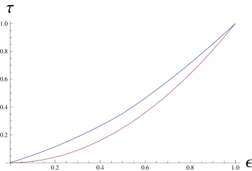
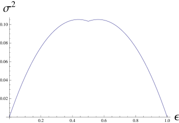
Figure 1: Boundary of the phase space for the 2-star case. Left: true phase boundary; Right: Plot of $\epsilon$ versus $\sigma^{2}=\tau-\epsilon^{2}$; in this case the lower boundary becomes the $x$-axis.

4.1 Proof of Theorem 4.1

The proof has three steps:

1. Showing that $g(x,y)$ only takes on the values 0 and 1.

2. Showing that $g$ is at most $3$-podal.

3. Showing that $g$ is bipodal. (This is the only step that uses $k\leq 30$.)

4.1.1 Step 1: Showing that we have a 0-1 graphon

The variational equation for maximizing $t_{k}(g)$ while fixing $t_{1}(g)$ is (see (20) without the ‘$\mathcal{S}$’ term)

$$d(x)^{k-1}+d(y)^{k-1}=\lambda$$ (40)

for some unknown constant $\lambda$, whenever $0<g(x,y)<1$. When $g(x,y)=0$ we have $d(x)^{k-1}+d(y)^{k-1}\leq\lambda$, and when $g(x,y)=1$ we have $d(x)^{k-1}+d(y)^{k-1}\geq\lambda$. Since $d(x)^{k-1}+d(y)^{k-1}$ is a decreasing function of both $x$ and $y$, this means that there is a strip (of possibly zero thickness) running roughly from the northwest corner of $[0,1]^{2}$ to the southeast corner, where $g(x,y)$ is strictly between 0 and 1, and where $d(x)^{k-1}+d(y)^{k-1}=\lambda$. All points to the southwest of this strip have $g(x,y)=1$, and all points to the northeast have $g(x,y)=0$. (The boundaries of the strip are necessarily monotone paths).

We claim that the strip has zero thickness, and hence is actually a boundary path between the $g=1$ zone and the $g=0$ zone. To see this, suppose that the strip contains a small ball, and hence contains a small rectangle. Since $d(x)^{k-1}+d(y)^{k-1}$ is constant on this rectangle, $d(x)$ is constant and $d(y)$ is constant. We can then increase the k-star density (i.e. $k$-th moment of $d(x)$) by moving some mass from right to left, and from top to bottom on the mirror image region, as in the proof of Theorem 3.4. As in that proof, this move increases $t_{k}(g)$ to second order in the amount of mass moved. Since we assumed that our graphon was a maximizer (and not just a stationary point), we have a contradiction.

4.1.2 Step 2: Showing $g$ is at most $3$-podal

By the above argument, the boundary between the region where $g=0$ and the region where $g=1$ is a monotone decreasing path $\gamma$ from $(0,1)$ to $(1,0)$, symmetric under reflection in $\{x=y\}$. Let $(c,c)$ be the point where it crosses the line $\{x=y\}$, and let $\gamma_{0}$ be the portion of $\gamma$ between $(0,1)$ and $(c,c)$. We compute

$$t_{k}= \int_{0}^{1}y^{k}dx d(x)=y(x)$$ since (41)

$$= \int_{\gamma_{0}}y^{k}dx-x^{k}dy$$ using reflection symmetry (42)

$$= -c^{k+1}+\int_{\gamma_{0}}(y^{k}+kx^{k-1}y)dx -x^{k}dy=kx^{k-1}ydx-d(x^{k}y)$$ since (43)

$$= -c^{k+1}+\int_{0}^{c}(y^{k}+kx^{k-1}y)dx dy$$ since there are no terms. (44)

Fix $c$. To maximize $t_{k}$ for this value of $c$ we need to maximize, over $y$, the above integral subject to the constraints that: first, $y=y(x)\in[c,1]$ is a non-increasing function of $x$, and second, the integral $\int_{0}^{c}ydx$ is fixed. If there are any nontrivial functions $\delta y(x)$ such that $\int_{0}^{c}\delta y(x)dx=0$ and such that $y(x)+t\delta y(x)$ is non-increasing (as a function of $x$) for all values of $t$ sufficiently close to 0, then $f(t)=\int_{0}^{c}(y+t\delta y)^{k}+kx^{k-1}(y+t\delta y)dx$ must have a local maximum at $t=0$. However, $f^{\prime\prime}(0)=k(k-1)\int_{0}^{c}y^{k-2}\delta y^{2}dx>0$. Thus such a function $\delta y$ cannot exist.

We now claim that $y$ takes at most one value between $c$ and $1$. Suppose that the range of $y$ includes two points $y_{1}$ and $y_{2}$ that are strictly between $c$ and $1$. That is, suppose the preimages of $(y_{i}-\epsilon,y_{i}+\epsilon)$ have positive measure for any $\epsilon>0$. Let $\phi_{1}$ and $\phi_{2}$ be a positive bump functions supported in non-overlapping $\epsilon$-neighborhoods of $y_{1}$ and $y_{2}$. Then take

$$\delta y(x)=C_{1}\phi_{1}(y(x))-C_{2}\phi_{2}(y(x)),$$ (45)

where the constants $C_{1}$ and $C_{2}$ are chosen so that $\int\delta y(x)dx=0$. Let $M$ be the maximal value of $|C_{i}\phi_{i}^{\prime}(y)|$, which is finite because $\phi_{i}$ is smooth. Then $y(x)+t\delta y(x)$ is monotonic for all $|t|<M^{-1}$, and thus $y$ is not maximal. This completes the proof of the claim.

Since $y$ takes at most one value between $c$ and $1$, $y(x)$ takes the form

$$y(x)=\begin{cases}1&x<x_{1},\cr y_{0}&x_{1}<x<x_{2},\cr c&x>x_{2}.\end{cases}$$ (46)

There are now several cases to consider.

• Suppose that $x_{2}<c$. Then we can vary $x_{2}$ and $y_{0}$ keeping $t_{1}$ and $c$ fixed to increase $t_{k}$: we write

  $$t_{k}=x_{1}^{k}(1-y_{0})+y_{0}^{k}(x_{2}-x_{1})+x_{2}^{k}(y_{0}-c)+c^{k}(c-x_{2})$$ (47)

  and substituting $x:=x_{2}-x_{1}$ and $z:=y_{0}-c$ this becomes

  $$t_{k}=-x_{1}^{k}z+(z+c)^{k}x+(x+x_{1})^{k}z-c^{k}x+constant$$ (48)

  and $t_{1}=2xz+constant$, where $constant$ refers to positive quantities independent of $x_{2},y_{0}$. Let $C=xz$ be fixed, so that $t_{1}$ is fixed. Then we have

  $$\frac{t_{k}}{C}=\frac{(z+c)^{k}-c^{k}}{z}+\frac{(x+x_{1})^{k}-x_{1}^{k}}{x}+constant$$ (49)

  which, replacing $x$ with $C_{2}/z$, is a polynomial in $z$ and $1/z$ with nonnegative coefficients, hence convex. It is thus maximized at the endpoints of definition of $x,z$, that is, $y_{0}=1$ or $x_{2}=c$.

• Suppose that $x_{2}=c$ and $x_{1}>0$. In this case we vary each of $x_{1},c,y_{0}$ forwards and backwards in “time” according to the differential equation

  $$\dot{x}_{1}(t)=\frac{\alpha}{1-y_{1}(t)},\qquad\dot{c}(t)=\frac{\beta}{y_{0}(t)-c(t)},\qquad\dot{y}_{0}(t)=\frac{\gamma}{c(t)-x_{1}(t)},$$ (50)

  where a dot denotes a derivative with respect to the time parameter $t$, and with constants $\alpha,\beta,\gamma$ satisfying $\alpha+\beta+\gamma=0$. Then $\dot{t}_{1}=0$. We will show that the second derivative $\ddot{t}_{k}$ is positive at $t=0$ for some choice of $\alpha,\beta,\gamma$, implying that we are not at a local maximum of $t_{k}$.

  We compute

  $$\dot{t}_{k}=\alpha(kx_{1}^{k-1}+\frac{1-y_{0}^{k}}{1-y_{0}})+\beta(kc^{k-1}+\frac{y_{0}^{k}-c^{k}}{y_{0}-c})+\gamma(ky_{0}^{k-1}+\frac{c^{k}-x_{1}^{k}}{c-x_{1}}).$$ (51)

  Differentiating again, we have

  $$\ddot{t}_{K}=\alpha^{2}A+\beta^{2}B+\gamma^{2}C+\alpha\gamma D+\beta\gamma E$$ (52)

  where the coefficients

  $$A = k(k-1)x_{1}^{k-2}/(1-y_{0}),$$ (53)

  $$B = (k(k-1)c^{k-2}+\frac{\partial}{\partial c}\frac{y_{0}^{k}-c^{k}}{y_{0}-c})/(y-c),$$ (54)

  $$C = k(k-1)y_{0}^{k-2}/(c-x_{1}),$$ (55)

  $$D = \frac{1}{c-x_{1}}\frac{\partial}{\partial y_{0}}\frac{1-y_{0}^{k}}{1-y_{0}}+\frac{1}{1-y_{0}}\frac{\partial}{\partial x_{1}}\frac{c^{k}-x_{1}^{k}}{c-x_{1}},$$ (56)

  $$E = \frac{1}{c-x_{1}}\frac{\partial}{\partial y_{0}}\frac{y_{0}^{k}-c^{k}}{y_{0}-c}+\frac{1}{y_{0}-c}\frac{\partial}{\partial c}\frac{c^{k}-x_{1}^{k}}{c-x_{1}},$$ (57)

  are all positive. Now taking $\alpha=-E$ and $\beta=D$ (evaluated at $t=0$) for example, the last two terms cancel and we find $\ddot{t}_{k}(0)>0$.

• If $x_{1}=0$ and $x_{2}=c$, $y(x)$ takes the form

  $$y(x)=\begin{cases}y_{0}&x<c,\cr c&c<x<y_{0},\cr 0&x>y_{0},\end{cases}$$ (58)

  In this case set $z=y_{0}/c$. We then have

  $$t_{1}=c^{2}(2z-1)$$ (59)

  $$t_{k}=cy_{0}^{k}+y_{0}c^{k}-c^{k+1}=c^{k+1}(z^{k}+z-1),$$ (60)

  which gives

  $$\frac{t_{k}}{t_{1}^{(k+1)/2}}=\frac{z^{k}+z-1}{(2z-1)^{(k+1)/2}}.$$ (61)

  This function of $z$ is unimodal for $z>1$ (decreasing, then increasing, as can be seen by replacing $z$ with $w=2z-1$) so the maximum of $t_{k}$ for fixed $t_{1}$ occurs at either $y_{0}=1$ or $y_{0}=c$, resulting in an anticlique or clique.

Thus $y$ cannot take any values strictly between $1$ and $c$.

Summarizing this section, we have shown that the path $\gamma_{0}$ from $(0,1)$ to $(c,c)$ must be first horizontal, then vertical, and then horizontal, although one of the horizontal segments can have zero length.

This implies that $g$ is either bipodal (a clique or anticlique) or tripodal, and if tripodal it is of the form

$$g(x,y)=\left\{\begin{array}[]{ll}1&x<c_{1}\\ c_{2}&c_{1}<x<c_{2}\\ c_{1}&c_{2}<x<1.\end{array}\right.$$ (62)

4.1.3 Step 3: Showing that $g$ is bipodal

If $g$ has the form (62), the edge and $k$-star densities are:

$$t_{1}=c_{1}+(c_{2}-c_{1})c_{2}+(1-c_{2})c_{1}=2c_{1}-2c_{1}c_{2}+c_{2}^{2}\qquad t_{k}=c_{1}+(c_{2}-c_{1})c_{2}^{k}+(1-c_{2})c_{1}^{k}.$$ (63)

Taking derivatives with respect to $c_{j}$ gives:

$$\partial_{1}t_{1}=2(1-c_{2}); \partial_{2}t_{1}=2(c_{2}-c_{1});$$ (64)

$$\partial_{1}t_{k}=1-c_{2}^{k}+k(1-c_{2})c_{1}^{k-1}; \partial_{2}t_{k}=(c_{2}^{k}-c_{1}^{k})+k(c_{2}-c_{1})c_{2}^{k-1}.$$ (65)

An important quantity is the ratio $r_{j}=2\frac{\partial_{j}t_{k}}{\partial_{j}t_{1}}$. For $j=1,2$, this works out to

$$r_{1} = kc_{1}^{k-1}+\frac{{1}-c_{2}^{k}}{{1}-c_{2}}$$ (66)

$$r_{2} = kc_{2}^{k-1}+\frac{c_{2}^{k}-c_{1}^{k}}{c_{2}-c_{1}}$$ (67)

We imagine $c_{1}$ and $c_{2}$ evolving in time so as to keep $t_{1}$ fixed, with $\dot{c}_{1}=c_{2}-c_{1},~{}~{}\dot{c}_{2}=c_{2}-{1}$ (note that this satisfies $\dot{t}_{1}=0$ by (64)). We must have $r_{1}=r_{2}$, or else $\dot{t}_{k}$ would be nonzero. We will show that then $d(r_{1}-r_{2})/dt>0$, and hence that $t_{k}$ increases to second order. We compute:

$$\dot{r}_{1}-\dot{r}_{2} = k(k-1)[c_{1}^{k-2}\dot{c}_{1}-c_{2}^{k-2}\dot{c}_{2}]$$ (70)

$$+k\left[-\frac{c_{1}^{k-1}\dot{c}_{2}}{{1}-c_{2}}-\frac{c_{2}^{k-1}\dot{c}_{2}}{c_{2}-c_{1}}+\frac{c_{1}^{k-1}\dot{c}_{1}}{c_{2}-c_{1}}\right]$$

$$+\frac{c_{2}^{k}-c_{1}^{k}}{c_{2}-c_{1}}\left[\frac{\dot{c}_{2}}{{1}-c_{2}}+\frac{\dot{c}_{2}}{c_{2}-c_{1}}-\frac{\dot{c}_{1}}{c_{2}-c_{1}}\right]$$

Plugging in the values of $\dot{c}_{1}$ and $\dot{c}_{2}$ then gives

$$\dot{r}_{1}-\dot{r}_{2} = k(k-1)\left[c_{1}^{k-2}(c_{2}-c_{1})+c_{2}^{k-2}(1-c_{2})\right]$$ (73)

$$+k\left[2c_{1}^{k-1}+c_{2}^{k-1}\frac{1-c_{2}}{c_{2}-c_{1}}\right]$$

$$-\frac{c_{2}^{k}-c_{1}^{k}}{c_{2}-c_{1}}\left[2+\frac{1-c_{2}}{c_{2}-c_{1}}\right]$$

Let $x=c_{1}/c_{2}$ and let $z=1/c_{2}$. Note that $x<1<z$. Then $\dot{r}_{1}-\dot{r}_{2}$ is $c_{2}^{k-1}$ times

$$f(x,z) := k(k-1)[x^{k-2}(1-x)+z-1]+k[2x^{k-1}+\frac{z-1}{1-x}]-\left(\frac{1-x^{k}}{1-x}\right)\left[2+\frac{z-1}{1-x}\right]$$ (74)

$$= k(k-1)[x^{k-2}(1-x)+z-1]+2[(k-1)x^{k-1}-x^{k-2}-\cdots-1]$$ (76)

$$+(z-1)[(k-1)+(k-2)x+\cdots+x^{k-2}].$$

This is an order $k-1$ polynomial in $x$ and linear in $z$. Likewise, the constraint $r_{1}=r_{2}$ becomes

$$0=F(x,z):=kx^{k-1}+\frac{z^{k}-1}{z-1}-k-\frac{1-x^{k}}{1-x}.$$ (77)

Note that $F(1,1)=f(1,1)=0$. By implicitly differentiating $F$ we see that $dx/dz=-1$ at $(x,z)=(1,1)$, hence that $df/dz|_{(1,1)}=\frac{3}{2}k(k-1)>0$. Hence $\dot{r}_{1}-\dot{r}_{2}$ is positive when $x$ is slightly less than 1. If $f(x,z)$ ever fails to be positive on the set where $F(x,z)=0$ then, by the intermediate value theorem, there is a value of $z$, and a corresponding value of $x$, for which $f(x,z)=0$ and $F(x,z)=0$. The intersection of the two degree $k-1$ algebraic curves $F=0$ and $f=0$ would then have to contain a real point $(x,z)$ with $0<x<1$.

This is easy to check. Solving $f(x,z)=0$ for $z$, we convert $F(x,z)$ into a function of $x$ alone. Plotting this function for $2\leq k\leq 30$ and $0<x<1$ shows that the function is always negative, approaching a simple zero at $x=1$; see Fig. 2 for plots of $F(x,z(x))$ as a function of $x$ for some $k$ values. (We were unable to prove this for all $k$; checking larger values of $k$ is straightforward, but we stopped at 30.) This eliminates the case (62) for $k\leq 30$.

We conclude this section with a qualitative feature of phase diagrams for models with constraints on edges and any other simple graph $H$.

Theorem 4.3.

The phase diagram for an edge-$H$ model is simply connected.

Proof.

This is just the intermediate value theorem. For each fixed edge density $\epsilon$, let $g_{\epsilon}$ be a graphon that maximizes $t_{H}$ and $h_{\epsilon}$ a graphon which minimizes $t_{H}$. Consider the family of graphons $m_{\epsilon,a}(x,y)=ah_{\epsilon}(x,y)+(1-a)g_{\epsilon}(x,y).$ When $a=0$ we get the maximal value of $t_{H}$, when $a=1$ we get the minimal value, and by continuity we have to get all values in between. In other words, the entire phase space between the upper boundary and the lower boundary is filled in. ∎

Note: This is an application of a technique we learned from Oleg Pikhurko [P].

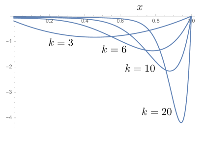
Figure 2: Plots of $F(x,z(x))$ as a function of $x$ for $k=3$, $k=6$, $k=10$ and $k=20$.

5 Phase Transition for $2$-Stars

Theorem 5.1.

For the 2-star model there are inequivalent graphons maximizing the constrained entropy on the line segment $\{(1/2,\tau_{2})\,|\,\tau^{*}<\tau_{2}\leq 2^{-3/2}\}$ for some $\tau^{*}<2^{-3/2}$. Moreover, near $(1/2,2^{-3/2})$, the maximizing graphons do not vary continuously with the constraint parameters.

Proof.

For any graphon $g$, consider the graphon $g^{\prime}(x,y)=1-g(x,y)$. The degree functions for $g^{\prime}$ and $g$ are related by $d^{\prime}(x)=1-d(x)$. If $g$ has edge and 2-star densities $\epsilon$ and $\tau_{2}$, then $g^{\prime}$ has edge density $1-\epsilon$ and 2-star density $\int_{0}^{1}(1-d(x))^{2}dx=1-2\epsilon+\tau_{2}$. Furthermore, $\mathcal{S}(g^{\prime})=\mathcal{S}(g)$. This implies that $g^{\prime}$ maximizes the entropy at $(1-\epsilon,1-2\epsilon+\tau_{2})$ if and only if $g$ maximizes the entropy at $(\epsilon,\tau_{2})$. In particular, if $g$ maximizes the entropy at $(1/2,\tau_{2})$, then so does $g^{\prime}$. To show that $\mathcal{S}(g)$ has a non-unique maximizer along the upper part of the $\epsilon=1/2$ line, we must only show that a maximizer $g$ is not related to its mirror $g^{\prime}$ by a measure-preserving transformation of $[0,1]$.

As noted in Section 4, up to such a transformation there are exactly two graphons corresponding to $(\epsilon,\tau_{2})=(1/2,1/({2\sqrt{2}}))$, namely a g-anticlique $g_{a}$ and a g-clique $g_{c}$. These are not related by reordering, since the values of the degree function for the g-clique are $\sqrt{2}/2$ and 0, while those for the g-anticlique are $1$ and $1-\sqrt{2}/2$. Let $D$ be smallest of the following distances in the cut metric (see Chapter 8 in [Lov]): (1) from $g_{a}$ to $g_{c}$, (2) from $g_{a}$ to the set of symmetric graphons, and (3) from $g_{c}$ to the set of symmetric graphons.

Lemma 5.2.

There exists $\delta>0$ such that every graphon with $(\epsilon,\tau_{2})$ within $\delta$ of $(1/2,2^{-3/2})$ is within $D/3$ of either $g_{a}$ or $g_{c}$.

Proof.

Suppose otherwise. Then we could find a sequence of graphons with $(\epsilon,\tau_{2})$ converging to $(1/2,2^{-3/2})$ that have neither $g_{a}$ nor $g_{c}$ as an accumulation point. However, the space of reduced graphons is known to be compact [Lov], so there must be some accumulation point $g_{\infty}$ that is neither $g_{a}$ nor $g_{c}$. Since convergence in the cut metric implies convergence of the density of all subgraphs, $t_{1}(g_{\infty})=1/2$ and $t_{2}(g_{\infty})=2^{-3/2}$. But this contradicts the fact that only $g_{a}$ and $g_{c}$ have edge and 2-star densities $(1/2,2^{-3/2})$. ∎

By the lemma, no graphon with $\epsilon=1/2$ and $\tau_{2}>1/2\sqrt{2}-\delta$ is invariant (up to reordering) under $g\to 1-g$. In particular, the entropy maximizers cannot be symmetric, so there must be two (or more) entropy maximizers, one close to $g_{a}$ and one close to $g_{c}$.

Moreover, on a path in the parameter space near the upper boundary, from the anticlique on the upper boundary at $\epsilon=\frac{1}{2}-\delta$ to the clique on the upper boundary at $\epsilon=1/2+\delta$, there is a discontinuity in the graphon, where it jumps from being close to $g_{a}$ to being close to $g_{c}$. There must be an odd number of such jumps, and if the path is chosen to be symmetric with respect to the transformation $\epsilon\to 1-\epsilon$, $\tau_{2}\to\tau_{2}+1-2\epsilon$, the jump points must be arranged symmetrically on the path. In particular, one of the jumps must be at exactly $\epsilon=1/2$. This shows that the $\epsilon=1/2$ line forms the boundary between a region where the optimal graphon is close to $g_{a}$ and another region where the optimal graphon is close to $g_{c}$. ∎

6 Simulations

We now show some numerical simulations in the 2-star model ($\ell=2,k_{1}=1,k_{2}=2$). Our main aim here is to present numerical evidence that the maximizing graphons in this case are in fact bipodal, and to clarify the significance of the degeneracy of Theorem 5.1.

To find maximizing $K$-podal graphons, we partition the interval $[0,1]$ into $K$ subintervals $\{I_{i}\}_{i=1,\dots,k}$ with lengths $c_{1},c_{2},\cdots,c_{K}$, that is, $I_{i}=[c_{0}+\dots+c_{i-1},c_{0}+\dots+c_{i}]$ (with $c_{0}=0$). We form a partition of the square $[0,1]^{2}$ using the product of this partition with itself. We are interested in functions $g$ that are piecewise constant on the partition:

$$g(x,y)=g_{ij},\ \ (x,y)\in I_{i}\times I_{j},\quad 1\leq i,j\leq K,$$ (78)

with $g_{ij}=g_{ji}$. We can then verify that the entropy density $\mathcal{S}(g)$, the edge density $t_{1}(g)$ and the 2-star density $t_{2}(g)$ become respectively

$$\mathcal{S}(g)=-\dfrac{1}{2}\displaystyle\sum_{1\leq i,j\leq K}[g_{ij}\log g_{ij}+(1-g_{ij})\log(1-g_{ij})]c_{i}c_{j},$$ (79)

$$t_{1}(g)=\displaystyle\sum_{1\leq i,j\leq K}g_{ij}c_{i}c_{j},\qquad t_{2}(g)=\displaystyle\sum_{1\leq i,j,k\leq K}g_{ik}g_{kj}c_{i}c_{j}.$$ (80)

Our objective is to solve the following maximization problem:

$$\max_{\{c_{j}\}_{1\leq j\leq K},\{g_{i,j}\}_{1\leq i,j\leq K}}\mathcal{S}(g),\quad\mbox{subject to:}\quad t_{1}(g)=\epsilon,\quad t_{2}(g)=\tau_{2},\quad\displaystyle\sum_{1\leq j\leq K}c_{j}=1,\quad g_{ij}=g_{ji}.$$ (81)

We developed in [RRS] computational algorithms for solving this maximization problem and have benchmarked the algorithms with theoretically known results. For a fixed $\tau\equiv(\epsilon,\tau_{2})$, our strategy is to first maximize for a fixed number $K$, and then maximize over the number $K$. Let $s_{(\epsilon,\tau_{2})}^{K}$ be the maximum achieved by the graphon $g_{{}_{K}}$, then the maximum of the original problem is $s_{(\epsilon,\tau_{2})}=\max_{K}\{s_{(\epsilon,\tau_{2})}^{K}\}$. Our computational resources allow us to go up to $K=16$ at this time. See [RRS] for more details on the algorithms and their benchmark with existing results.

The most important numerical finding in this work is that, for every pair $(\epsilon,\tau_{2})$ in the interior of the phase space, the graphons that maximize $\mathcal{S}(g)$ are bipodal. We need only four parameters ($c_{1}$, $g_{11}$, $g_{12}$ and $g_{22}$) to describe bipodal graphons (due to the fact that $c_{2}=1-c_{1}$ and $g_{12}=g_{21}$). For maximizing bipodal graphons, we need only three parameters, since (28) implies that

$$\left(\frac{1}{g_{11}}-1\right)\left(\frac{1}{g_{22}}-1\right)=\left(\frac{1}{g_{12}}-1\right)^{2},$$ (82)

which was used in our numerical algorithms to simplify the calculations.

We show in Fig. 3 maximizing graphons at some typical points in the phase space. The $(\epsilon,\tau_{2})$ pairs for the plots are respectively: $(0.3,0.16844286)$ and $(0.3,0.10339268)$ for the first column (top to bottom), $(0.5,0.32455844)$ and $(0.5,0.27485281)$ for the second column, and $(0.7,0.56270313)$ and $(0.7,0.50339268)$ for the third column.

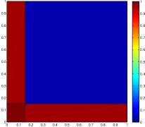
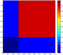
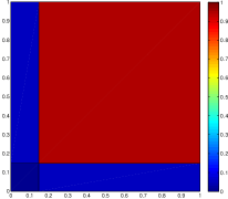
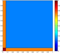
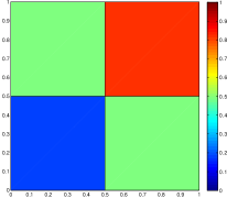
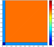
Figure 3: Maximizing graphons at $\epsilon=0.3$ (left column), $\epsilon=0.5$ (middle column) and $\epsilon=0.7$ (right column). For each column $\tau_{2}$ values decrease from top to bottom.

The values of $s$ corresponding to the maximizing graphons are shown in the left plot of Fig. 4 for a fine grid of $(\epsilon,\sigma^{2})$ (with $\sigma^{2}=\tau_{2}-\epsilon^{2}$ as defined in Fig. 1) pairs in the phase space. We first observe that the plot is symmetric with respect to $\epsilon=1/2$. The symmetry comes from the fact (see the proof of Theorem 5.1) that the map $g\to 1-g$ takes $\epsilon\to 1-\epsilon$, $\tau_{2}\to 1-2\epsilon+\tau_{2}$ and thus $\sigma^{2}\to\sigma^{2}$. To visualize the landscape of $s$ better in the phase space, we also show the cross-sections of $s_{(\epsilon,\tau_{2})}(\epsilon,\sigma^{2})$ along the lines $\epsilon_{k}=0.05k$, $k=7,\cdots,13$, in the right plots of Fig. 4.

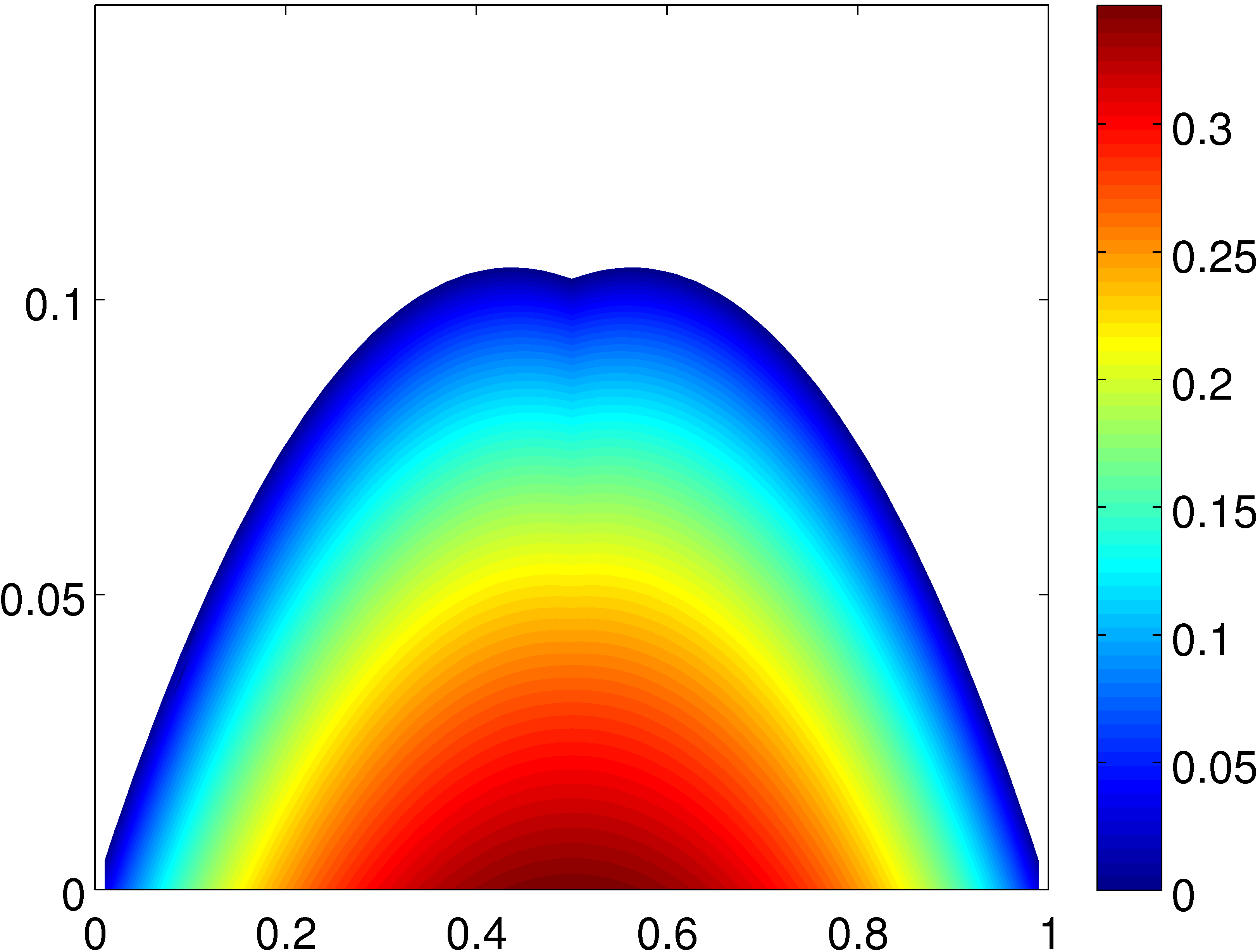
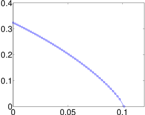
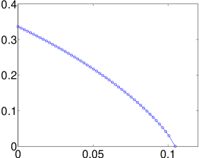
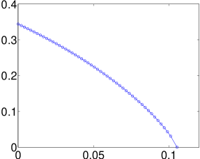
Figure 4: Left: values of $s_{(\epsilon,\tau_{2})}$ at different $(\epsilon,\sigma^{2})$ pairs; Right: cross-sections of $s_{(\epsilon,\tau_{2})}(\epsilon,\sigma^{2})$ along lines $\epsilon=\epsilon_{k}=0.05k$ ($k=7,\cdots,13$) (from top left to bottom right).

We show in the left plot of Fig. 5 the values of $c_{1}$ of the maximizing graphons as a function of the pair $(\epsilon,\sigma^{2})$. Here we associate $c_{1}$ with the set of vertices among $V_{1}$ and $V_{2}$ that has the larger probability of an interior edge. This is done to avoid the ambiguity caused by the fact that one can relabel $V_{1}$, $V_{2}$ and exchange $c_{1}$ and $c_{2}$ to get an equivalent graphon with the same $\epsilon$, $\tau_{2}$ and $\mathcal{S}$ values. We again observe the symmetry with respect to $\epsilon=1/2$. The cross-sections of $c_{1}(\epsilon,\sigma^{2})$ along the lines of $\epsilon_{k}=0.05k$ ($k=7,\cdots,13$) are shown in the right plots of Fig. 5.

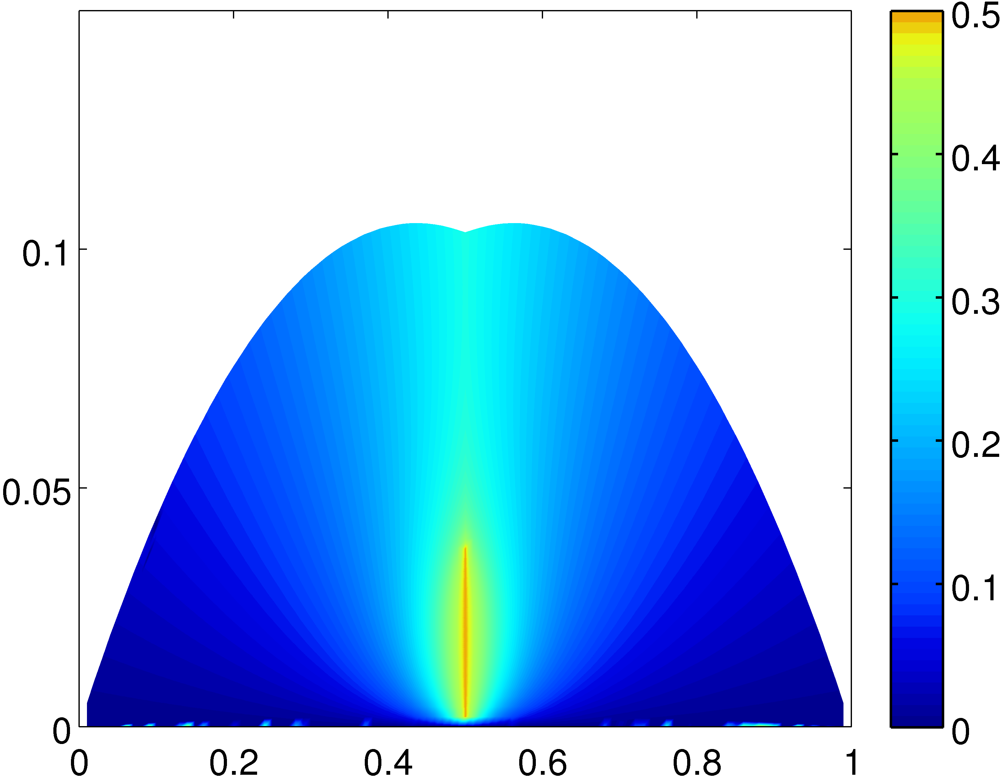
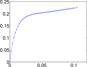
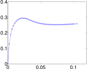
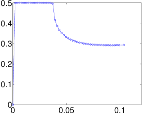
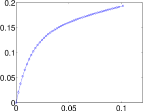
Figure 5: Left: $c_{1}$ of the maximizing bipodal graphons as a function of $(\epsilon,\sigma^{2})$; Right: cross-sections of $c_{1}(\epsilon,\sigma^{2})$ along lines of $\epsilon_{k}=0.05k$ ($k=7,\cdots,13$).

The last set of numerical simulations were devoted to the study of a phase transition in the 2-star model. The existence of this phase transition is suggested by the degeneracy in Theorem 5.1. Our numerical simulations indicate that the functions differ to first order in $\epsilon-1/2$, and that the actual entropy $s_{(\epsilon,\tau_{2})}=\max\{{s^{L}}_{(\epsilon,\tau_{2})},s^{R}_{(\epsilon,\tau_{2})}\}$ has a discontinuity in $\partial_{\epsilon}s_{(\epsilon,\tau_{2})}$ at $\epsilon=1/2$ above a critical value $\tau_{2}^{c}$. Below $\tau_{2}^{c}$, there is a single maximizer, of the form

$$g(x,y)=\begin{cases}\frac{1}{2}+\nu&x,y<\frac{1}{2}\cr\frac{1}{2}-\nu&x,y>\frac{1}{2}\cr\frac{1}{2}&\hbox{otherwise}\end{cases}$$ (83)

Here $\nu$ is a parameter related to $\tau_{2}$ by $\tau_{2}=1/4+{\nu^{2}}/{4}$. Applying the symmetry $g\to 1-g$ and reordering the interval $[0,1]$ by $x\to 1-x$ sends $g$ to itself.

The critical point $\tau_{2}^{c}$ is located on the boundary of the region in which the maximizer (83) is stable. The value of $\tau_{2}^{c}$ can be found by computing the second variation of $\mathcal{S}(g)$ within the space of bipodal graphons with fixed values of $(\epsilon=\frac{1}{2},\tau_{2})$, evaluated at the maximizer (83). This second variation is positive-definite for $\nu$ small (i.e. for $\tau_{2}$ close to $1/4$) and becomes indefinite for larger values of $\nu$. At the critical value of $\tau_{2}^{c}$, $\nu=2\sqrt{\tau_{2}^{c}-1/4}$ satisfies

$$\left(2S(\frac{1}{2}-\nu)-2S(\frac{1}{2})+3\nu S^{\prime}(\frac{1}{2}-\nu)\right)(2-\frac{1}{2}S^{\prime\prime}(\frac{1}{2}-\nu))+8\nu^{2}S^{\prime\prime}(\frac{1}{2}-\nu)=0$$ (84)

where $S^{\prime}$ and $S^{\prime\prime}$ are respectively the first and second order derivatives of $S(g)$ (defined in (6)) with respect to $g$. This equation is transcendental, and so cannot be solved in closed form. Solving it numerically for $\nu$ leads to the value $\tau_{2}^{c}\approx 0.287$, or $\sigma^{2}\approx 0.037$. This agrees precisely with what we previously observed in our simulations of optimizing graphons, and corresponds to the point in the left plot Fig. 5 where the $c_{1}=1/2$ region stops.

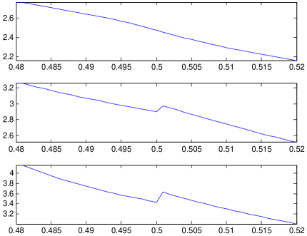
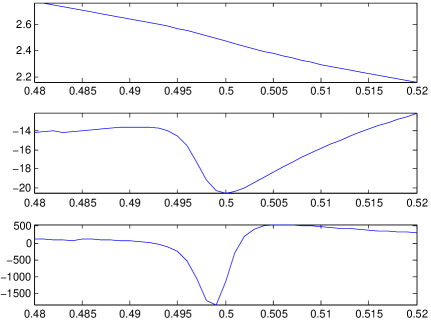
Figure 6: Left: the derivative $\frac{\partial s_{(\epsilon,\tau_{2})}}{\partial\epsilon}$ at $\tau_{2}=0.28$ (top), $\tau_{2}=0.30$ (middle) and $\tau_{2}=0.32$ (bottom) in the neighborhood of $\epsilon=0.5$; Right: the derivatives $\frac{\partial s_{(\epsilon,\tau_{2})}}{\partial\epsilon}$ (top), $\frac{\partial^{2}s_{(\epsilon,\tau_{2})}}{\partial\epsilon^{2}}$ (middle) and $\frac{\partial^{3}s_{(\epsilon,\tau_{2})}}{\partial\epsilon^{3}}$ (bottom) in the neighborhood of $\epsilon=0.5$ for $\tau_{2}=0.28$.

In the left plot of Fig. 6, we show numerically computed derivatives of $s_{(\epsilon,\tau_{2})}$ with respect to $\epsilon$ in the neighborhood of $\epsilon=0.5$ for three different values of $\tau_{2}$: one below the critical point and two above it. It is clear that discontinuities in the first order derivative of $s$ appears at $\epsilon=0.5$ for $\tau_{2}>\tau_{2}^{c}$. When $\tau_{2}<\tau_{2}^{c}$, we do not observe any discontinuity in the first three derivatives of $s$.

7 The Taco Model

We next compute the phase space of a model with constrained densities of $k$-stars for $k=1,2,3$. We call this the “taco” model from the shape of its phase space; see Figure 8. Let $t_{k}$ be the density of $k$-stars.

A simple application of the Cauchy-Schwarz inequality applied to $d^{1/2}$ and $d^{3/2}$ shows that

$$t_{1}t_{3}\geq t_{2}^{2}.$$ (85)

Under the symmetry $g(x,y)\to 1-g(x,y)$ we have

$$t_{1} \to 1-t_{1},$$ (86)

$$t_{2} \to 1-2t_{1}+t_{2},$$ (87)

$$t_{3} \to 1-3t_{1}+3t_{2}-t_{3}.$$ (88)

The inequality (85) thus gives another inequality

$$(1-t_{1})(1-3t_{1}+3t_{2}-t_{3})\geq(1-2t_{1}+t_{2})^{2}.$$ (89)

These two inequalities (or more precisely, the corresponding equalities) form two boundaries of the phase space. The rest of the boundary is determined by an Euler-Lagrange equation, and is given by the locus of values obtained by the tripodal $\{0,1\}$-valued graphons of Figure 7, right, when $x_{1},x_{2},x_{3}$ vary over all possible values with $x_{1}+x_{2}+x_{3}=1$.

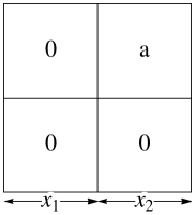
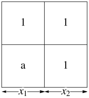
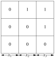
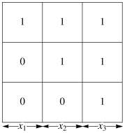
Figure 7: Graphons defining the boundary of the phase space.

Theorem 7.1.

The phase space of $t_{1},t_{2},t_{3}$-values of graphons is the solid domain delimited by these four algebraic surfaces. See Figure 8. Its boundary is piecewise analytic with four pieces; the four families of graphons parameterized by the four pieces are indicated in Figure 7.

The two upper surfaces (corresponding to the two right graphons in Figure 7) meet along three algebraic curves: one corresponding to $a=1$ in the first graphon (the curve along the top of the front part of the “shell” of the taco), one corresponding to $a=0$ in the second graphon (the curve along the top of the back part of the shell) and a third curve running along the center of the taco. Along this third curve we have two inequivalent graphons. This coexistence curve is a high-degree algebraic curve in $x_{1},x_{2},x_{3}$.

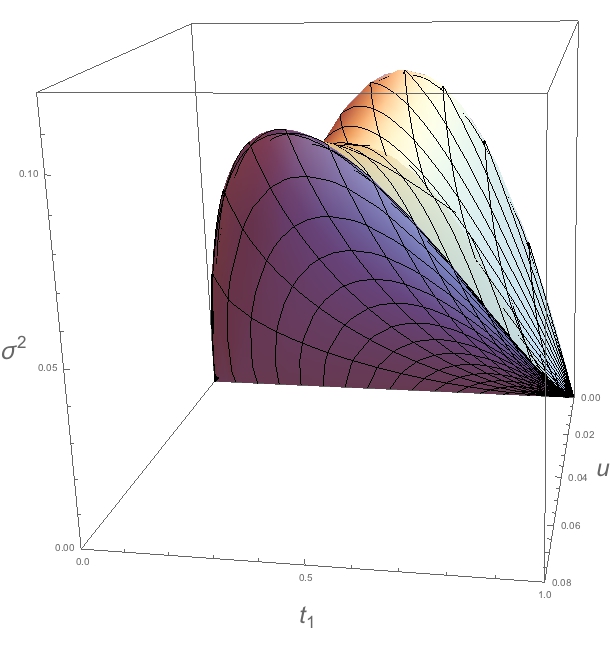
Figure 8: The phase space, or “taco”. The axes are $t_{1},\sigma^{2}=t_{2}-t_{1}^{2},$ and $u=t_{3}-t_{2}^{2}/t_{1}$. The front (dark shaded) face is the surface defined by the equality in (89). The back face (flush with the back boundary $u=0$) is defined by equality in (85). The “upper” faces are surfaces defined by the tripodal $0-1$-valued graphons of Figure 7, right. Note that if we project the taco along the $u$ direction we get Figure 1, right; one sees that the coexistence line there in fact lifts to two different curves in the taco phase space.

I’m inserting a new proof, more or less from scratch, but am leaving the older proof intact.

Proof.

The two graphon families on the left in Figure 7 correspond to $t_{1},t_{2},t_{3}$-values satisfying equality in (85) and (89), respectively, so they indeed comprise part of the boundary of the phase space. We need to verify only that there are no graphons above the “upper” boundaries.

By Theorem 3.1 we may assume that $d(x)$ is monotone increasing and $g(x,y)$ is monotone increasing in both variables. We fix $t_{1}$ and $t_{3}$ and look for extremal values of $t_{2}$. Our goal is to show that if $t_{2}$ is maximized, then the form of $g$ is either that of the first graphon in Figure 7 or of the last two (possibly with one of the podes having zero width). Likewise, if we minimize $t_{2}$ for fixed $t_{1}$ and $t_{2}$ we get the form of the second graphon.

First we limit the number of distinct values that the degree function $d(x)$ can take.

Lemma 7.2.

Suppose that $x_{1}<x_{2}<x_{3}$ and that $d(x_{2})<d(x_{3})$ and that there exists a $y$ such that $0<g(x_{1},y)\leq(g(x_{2},y)<1$. Then the graphon does not maximize $t_{2}$ for fixed $t_{1}$ and $t_{3}$.

Proof.

Since $d(x)$ is monotonic, we much have $d(x_{1})\leq d(x_{2})<d(x_{3})$. We first rule out the possibility that $d(x_{1})<d(x_{2})$, and then the possiblity that $d(x_{1})=d(x_{2})$. In all cases we consider the change to $t_{1}$, $t_{2}$ and $t_{3}$ from moving mass.

Since $t_{k}=\int_{0}^{1}d(x)^{k}dx$, changing the degree function $d(x)$ to $d(x)+\Delta d(x)$ results in the following changes to the dentisites:

$$\Delta t_{1} = \int_{0}^{1}\Delta d(x)dx$$ (90)

$$\Delta t_{2} = \int_{0}^{1}2d(x)\Delta d(x)+\Delta d(x)^{2}dx$$ (91)

$$\Delta t_{3} = \int_{0}^{1}3d(x)^{2}\Delta d(x)+3d(x)\Delta d(x)^{2}+\Delta d(x)^{3}dx$$ (92)

We consider the effect of moving mass from near $(x_{3},y)$ to near $(x_{2},y)$, thereby decreasing $d(x)$ near $x=x_{3}$ and increasing $d(x)$ near $x=x_{2}$. (To maintain symmetry we must also move mass from $(y,x_{3})$ to $(y,x_{2})$, but that does not affect the degree function.) If the amount of mass moved is $\epsilon$, then

$$\Delta t_{1} = 0$$ (93)

$$\Delta t_{2} = \epsilon 2(d(x_{2})-d(x_{3}))+O(\epsilon^{2})$$ (94)

$$\Delta t_{3} = \epsilon 3(d(x_{2})^{2}-d(x_{3})^{2}).$$ (95)

Note that $\Delta t_{2}/\Delta t_{3}\approx\frac{2}{3(d(x_{2})+d(x_{3}))}$. If $d(x_{1})<d(x_{2})$, then we can increase $t_{2}$ and $t_{3}$ by moving mass $\epsilon^{\prime}$ from $(x_{1},y)$ to $(x_{2},y)$ and in this case $\Delta t_{2}/\Delta t_{3}\approx\frac{2}{3(d(x_{1})+d(x_{2})}$, which is strictly larger than $\frac{2}{3(d(x_{2})+d(x_{3}))}$. By combining the two moves with $\epsilon^{\prime}=\frac{d(x_{3})^{2}-d(x_{2})^{2}}{d(x_{2})^{2}-d(x_{1})^{2}}\epsilon+O(\epsilon^{2})$, we can obtain $\Delta t_{1}=\Delta t_{3}=0$ and $\Delta t_{2}>0$, which shows that $t_{2}$ is not maximized.

If $d(x_{1})=d(x_{2})$, then moving mass from $(x_{1},y)$ to $(x_{2},y)$ only changes $t_{2}$ and $t_{3}$ to second order in $\epsilon^{\prime}$, but we still have $\Delta t_{2}/\Delta t_{3}\approx\frac{1}{3d(x_{1})}$, which is still strictly larger than $\frac{2}{3(d(x_{2})+d(x_{3}))}$. By taking $\epsilon^{\prime}$ of order $\sqrt{\epsilon}$ (with the exact constant depending on the details of the transport), we can again obtain $\Delta t_{1}=\Delta t_{3}=0$ and $\Delta t_{2}>0$.

∎

It follows from the lemma that if $g$ is a graphon that maximizes $t_{2}$, then either

• $g(x,y)=0$ or 1 almost everywhere, a possiblility that will be explored further below, or

• There is only one value of $d(x)$ corresponding to $x$’s for which $0<g(x,y)<1$, and there are no larger values of $d(x)$. In this case, we must have the first graphon shown in Figure 7. Note that in this case $t_{2}=\sqrt{t_{1}t_{3}}$, and is in fact maximal.

We now assume that $g$ takes values only in $\{0,1\}$, and, reversing our convention for the rest of the proof, is monotone decreasing in both variables.

As in the proof of Theorem 4.1, we consider the boundary between the regions where $g=1$ and $g=0$; it is a montone path in $[0,1]^{2}$ from $(0,1)$ to $(1,0)$ symmetric with respect to the line $\{x=y\}$. Consider the upper part of the path from $(0,1)$ to $(c,c)$. As in the proof of Theorem 4.1, the path necessarily maximizes the integral $\int_{0}^{c}y^{2}+2xy\,dx$ subject to the constraints of constant integrals of $y\,dx$ and $y^{3}+3x^{2}y\,dx$. We consider several possibilities.

1. If $y$ only takes one value for $x\in(0,c)$, or only takes on the values 1 and $c$, then we have either the third or fourth graphon in Figure 7 (possibly with one of the three regions having zero width).

2. In all other cases, we are neither at a stationary point of $t_{2}$ (for fixed $t_{1}$) nor a stationary point of $t_{3}$. In this case we can use the method of Lagrange multipliers . If we vary the path from $(0,1)$ to $(c,c)$, while holding $c$ fixed, then the (first-order) variations in $t_{1}$, $t_{2}$ and $t_{3}$ are:

   $$\delta t_{1} = \int_{0}^{c}2\delta ydx$$ (96)

   $$\delta t_{2} = \int_{0}^{c}2(y+x)\delta ydx$$ (97)

   $$\delta t_{3} = \int_{0}^{c}3(y^{2}+x^{2})\delta ydx$$ (98)

   There must exist constants $\alpha$ and $\beta$ such that $\delta t_{3}=\alpha\delta t_{1}+\beta\delta t_{3}$ for all possible variations $\delta y$. This means that our boundary is the circle

   $$x+y=\alpha+\frac{3\beta}{2}(x^{2}+y^{2}).$$ (99)

   Furthermore, by varying $y$ we can vary any two of $(t_{1},t_{2},t_{3})$ freely, with the third determined by the other two.

   Here’s where I need to check my algebra. I think the answer is basically to do a variation of size $\epsilon^{\prime}$ that doesn’t change any of the densities to first order, but that increases $t_{2}$ and $t_{3}$ to second order. Then do a move, of size $\epsilon=O(\epsilon^{\prime}{}^{2})$, that changes both $t_{2}$ and $t_{3}$ to first order in $\epsilon$ (hence second order in $\epsilon^{\prime}$). If the ratios $\Delta t_{3}/\Delta t_{2}$ satisfy some inequalities, we can piece it all together to get a variation that keeps $t_{1}$ and $t_{3}$ fixed and increases $t_{2}$.

∎

Proof.

The two graphon families on the left in Figure 7 correspond to $t_{1},t_{2},t_{3}$-values satisfying equality in (85) and (89), respectively, so they indeed comprise part of the boundary of the phase space. We need to verify only that there are no graphons above the “upper” boundaries.

By Theorem 3.1 we may assume that $d(x)$ is monotone increasing and $g(x,y)$ is monotone increasing in both variables.

Now fix $t_{1},t_{3}$ and take $t_{2}$ maximal. Our goal is to show that $g$ is then one of the two graphons on the right in Figure 7. We first show that $g$ only takes values in $\{0,1\}$. To accomplish this, we show first that if $g(x,y)\in(0,1)$ on a positive measure set, then $d$ can take at most $2$ values, then show that $d$ can in fact take at most one value (which would mean the graphon is an Erdős-Renyi graphon).

Suppose that $g(x,y)\in(0,1)$ on a positive measure set; then by montonicity $g\in(0,1)$ on an open set containing a rectangle $R_{1}=[x^{\prime},x^{\prime\prime}]\times[y^{\prime},y^{\prime\prime}]$.

Suppose now that $d$ takes at least three values on $(0,1)$.

• If $d(x)$ takes at least two values on $R_{1}$, we can find $x_{1},x_{2}\in[x^{\prime},x^{\prime\prime}]$ and $x_{3}\in[0,1]$ such that $d(x_{1})<d(x_{2})<d(x_{3})$ or $d(x_{3})<d(x_{1})<d(x_{2})$ (again using montonicity). Suppose we are in the first case; the second is similar. By shifting mass $\delta$ from $g(x_{1},y)$ to $g(x_{2},y)$ and $\varepsilon$ from $g(x_{3},y)$ to $g(x_{2},y)$, where

  $$\varepsilon=\frac{d(x_{2})^{2}-d(x_{1})^{2}}{d(x_{3})^{2}-d(x_{2})^{2}}\delta+O(\delta)^{2}$$ (100)

  we can fix $t_{1},t_{3}$ while increasing $t_{2}$; a short calculation yields

  $$\Delta t_{2}=\frac{(d(x_{2})-d(x_{1}))(d(x_{3})-d(x_{1}))}{d(x_{2})+d(x_{3})}\delta+O(\delta^{2}).$$ (101)

  This contradicts maximality.

• Suppose that $d(x)$ is constant on $R_{1}$. Let $(x_{1},y_{1}),(x_{2},y_{1})\in R_{1}$ and find a point $(x_{3},y_{1})\not\in R_{1}$ with $d(x_{3})\neq d(x_{1})$. We assume $d(x_{3})>d(x_{1})$, the other case is similar. Since $x_{3}>x_{1}$ by monotonicity, $g(x_{3},y_{1})>0$. We move mass $\varepsilon$ from $(x_{3},y_{1})$ to $(x_{1},y_{1})$, and mass $\delta$ from $(x_{2},y_{1})$ to $(x_{1},y_{1})$. Here we let $\varepsilon$ be of order $\delta^{2}$. The changes in $t_{3}$ and $t_{2}$ are then respectively

  $$\Delta t_{3} = 3\varepsilon(-d(x_{3})^{2}+d(x_{1})^{2})+6\delta^{2}d(x_{1})+O(\delta^{3})$$ (102)

  $$\Delta t_{2} = 2\varepsilon(-d(x_{3})+d(x_{1}))+2\delta^{2}.$$ (103)

  In particular by setting

  $$\varepsilon=\frac{2d(x_{1})\delta^{2}}{d(x_{3})^{2}-d(x_{1})^{2}}+O(\delta^{3})$$ (104)

  we can fix $t_{3}$ while increasing $t_{2}$: with this value of $\varepsilon$,

  $$\Delta t_{2}=\frac{2(d(x_{3})-d(x_{1}))\delta^{2}}{d(x_{3})+d(x_{1})}.$$ (105)

  This contradicts maximality of $t_{2}$.

This completes the proof of the claim that $d$ takes at most $2$ values globally. However the argument of the second bullet point shows in fact that either $d$ takes only one value, or $g$ takes values only in $\{0,1\}$. Thus we may assume $g$ takes values only in $\{0,1\}$.

We now assume that $g$ takes values only in $\{0,1\}$, and, reversing our convention for the rest of the proof, is monotone decreasing in both variables.

As in the proof of Theorem 4.1, we consider the boundary between the regions where $g=1$ and $g=0$; it is a montone path in $[0,1]^{2}$ from $(0,1)$ to $(1,0)$ symmetric with respect to the line $\{x=y\}$. Consider the upper part of the path from $(0,1)$ to $(c,c)$. As in the proof of Theorem 4.1, the path necessarily maximizes the integral $\int_{0}^{c}y^{2}+2xy\,dx$ subject to the constraints of constant integrals of $y\,dx$ and $y^{3}+3x^{2}y\,dx$. By the method of Lagrange multipliers we find that $y$ can take at most $2$ values: the endpoints $c,1$ or the roots of the derivative

$$\frac{d}{dy}(y^{2}+2xy+\lambda_{1}y+\lambda_{2}(y^{3}+3x^{2}y))$$ (106)

which, being a quadratic polynomial, has at most two roots.

Thus we can assume that $g$ is at worst $5$-podal.

We conclude [missing argument] that $t_{2}$ is maximized only when it is tripodal, that is, $g$ (reordered to be increasing) has one of the two forms of Figure 7, right.

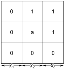
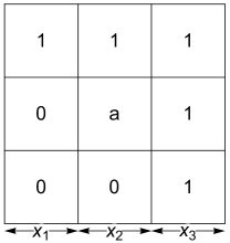
Figure 9: Graphons covering the interior of the taco.

It remains to show that the taco is full, that is, each interior point is realizable. We consider the $3$-parameter family $\Omega$ of tripodal graphons of Figure 9 (left). This family maps into $t_{1},t_{2},t_{3}$-space with Jacobian nonzero on the interior: the Jacobian is

$$(a-1)^{2}x_{2}^{4}\left(a^{2}x_{2}^{3}+2a^{2}x_{3}x_{2}^{2}+2ax_{3}^{2}x_{2}+x_{3}x_{2}^{2}+x_{3}^{2}x_{2}+x_{3}^{3}\right)$$ (107)

which is a sum of positive terms. Moreover the boundary of $\Omega$ maps to the part of the taco boundary consisting of three of the faces of the taco, only missing an area below one of the upper faces (see Figure 10). The map is thus a homeomorphism on the interior of $\Omega$ to the interior of its image. Now let $\Omega^{\prime}$ be the image of $\Omega$ under the involution, or equivalently, the graphons from Figure 9 (right); this covers the remaining part of the taco. ∎

Figure 10: The image of the upper boundary of $\Omega$; shown in transparent rendering is the other half of the upper boundary of the taco, which is part of the boundary of the image of $\Omega^{\prime}$.

8 A Finitely Forced Model

We have shown that, in the interior of the phase space, entropy maximizers with edge and $k$-star densities as constraints are multipodal. It is known from extremal graph theory that this is not true in general on the boundary of the phase space. We now briefly look at this issue using the concept of finitely forcible graphons introduced in [LS3].

Let $h(x,y)$ be any doubly monotonic function with 0 as a regular value, and consider the graphon

$$g(x,y)=\begin{cases}1&h(x,y)>0\cr 0&h(x,y)<0\end{cases}.$$ (108)

Then it is shown in [LS3] that for this graphon, the density of the signed quadrilateral subgraph $Q$ (with signs going around the quadrilateral as $+$, $-$, $+$, $-$), is zero. In other words,

$$t_{Q}(g)=\int g(w,x)[1-g(x,y)]g(y,z)[1-g(w,z)]dw\,dx\,dy\,dz=0,$$ (109)

where we have labelled the four vertices as $w,x,y,z$. It is straightforward to verify that $t_{Q}=t_{1}^{2}-2\tilde{t}_{3}+\tilde{t}_{4}$ where $\tilde{t}_{3}$ is the density of 3-chains while $\tilde{t}_{4}$ is the density of the un-signed quadrilateral:

$$\begin{array}[]{rcl}\tilde{t}_{3}(g)&=&\int g(w,x)g(x,y)g(y,z)dw\,dx\,dy\,dz,\\ \tilde{t}_{4}(g)&=&\int g(w,x)g(x,y)g(y,z)g(z,w)dw\,dx\,dy\,dz.\end{array}$$ (110)

The triangle graphon $g_{T}$ defined by

$$g_{T}(x,y)=\begin{cases}1&x+y>1\cr 0&x+y<1\end{cases}$$ (111)

is a special case of (108) with $h(x,y)=x+y-1$. For the triangle graphon we check that it has edge density $t_{1}=1/2$, 2-star density $t_{2}=1/3$, 3-chain density $\tilde{t}_{3}=5/24$ and quadrilateral density $\tilde{t}_{4}=1/6$. This clearly gives us $t_{Q}(g_{T})=0$.

It is shown in [LS3] that (up to rearranging vertices) graphons of the form (108) are the only kind of graphon for which $t_{Q}(g)=0$. Moreover, among graphons of the form (108) the density of edges minus the density of 2-stars is at most 1/6, and this upper bound is achieved uniquely by the graphon $g_{T}$. Thus the triangle graphon $g_{T}$ is finitely forcible with the two constraints:

1. $\zeta_{1}(g)\equiv t_{1}(g)-t_{2}(g)-\frac{1}{6}\geq 0$, i.e. the density of edges should be 1/6 greater than the density of 2-stars.

2. $\zeta_{2}(g)\equiv t_{Q}(g)=t_{1}^{2}(g)-2\tilde{t}_{3}(g)+\tilde{t}_{4}(g)=0$, i.e. the density of the signed quadrilateral subgraph $Q$ should be zero.

Here we look at a path toward the triangle graphon by considering the parameterized family of graphons $g_{\alpha}(x,y)=\alpha+(1-2\alpha)g_{T}(x,y)$ ($0\leq\alpha\leq 0.5$). We attempt to maximize the entropy among graphons that have the same values of ${t}=(t_{1},t_{2},\tilde{t}_{3},\tilde{t}_{4})$ as $g_{\alpha}$. We first check that

$$t_{1} = 1/2$$ (112)

$$t_{2} = (1-\alpha+\alpha^{2})/3$$ (113)

$$\tilde{t}_{3} = (5-8\alpha+8\alpha^{2})/24$$ (114)

$$\tilde{t}_{4} = (1-3\alpha+5\alpha^{2}-4\alpha^{3}+2\alpha^{4})/6.$$ (115)

This gives $\zeta_{1}(g_{\alpha})=\alpha(1-\alpha)/3$ and $\zeta_{2}(g_{\alpha})=\alpha(1+\alpha-4\alpha^{2}+2\alpha^{3})/6$.

We can show that by enforcing the densities $(t_{1},t_{2},\tilde{t}_{3},\tilde{t}_{4})$, we are approaching the triangle graphon from the interior of the profile when we let $\alpha\to 0$, as stated in the following theorem.

Theorem 8.1.

For any $\alpha>0$, the values of $t$ lie in the interior of the profile.

Proof.

Since the graphon $g_{a}$ is strictly between 0 and 1, it is enough to show that the four functional derivatives, $\delta t_{1}/\delta g$, $\delta t_{2}/\delta g$, $\delta\tilde{t}_{3}/\delta g$ and $\delta\tilde{t}_{4}/\delta g$, are linearly independent functions of $x$ and $y$, since then by varying $g$ we can change ${t}$ in any direction to first order. A simple computation shows that $\delta t_{1}/\delta g(x,y)$ is a constant, $\delta t_{2}/\delta g(x,y)$ is a linear polynomial in $x$ and $y$, and $\delta\tilde{t}_{3}/\delta g(x,y)$ is a quadratic polynomial with an $xy$ term as well as linear terms. These three are analytic and manifestly linearly independent.

However, $\delta\tilde{t}_{4}/\delta g(x,y)$ is not analytic across the line $x+y=1$, and so cannot be a linear combination of the first three functional derivatives. To see this, it is enough to consider the case of $\alpha=0$. $\delta t_{4}/\delta g(x,y)$ is a multiple of the probability of $x$ being connected to $y$ via a 3-chain $y$-$z$-$w$-$x$. When $x+y<1$, this is exactly $xy$, since if $z>1-y$ and $w>1-x$ then $z+w$ is automatically greater than $1$. When $x+y>1$, the requirement that $z+w>1$ provides an extra condition, and the functional derivative is strictly less than $xy$. ∎

We can now show that if we try to fit the density $t$ with $M$-podal graphons, then $M$ blows up as $\alpha$ goes to zero. More precisely,

Theorem 8.2.

For each positive integer $M$ there is an $\epsilon_{M}>0$ such that for $\alpha<\epsilon_{M}$ there are no $M$-podal graphons whose densities ${t}$ are the same as those of $g_{\alpha}$.

Proof.

Suppose otherwise. Then we could find $M$-podal graphons for arbitrarily small $\alpha$. Since the space of $M$-podal (or smaller) graphons is compact, we can find a subsequence that converges to $g_{0}$ as $\alpha\to 0$. But densities vary continuously with the graphon, being simply integrals of products of $g$’s. So the densities of the $M$-podal graphon $g_{0}$ are the same as the densities of $g_{T}$. But that is a contradiction, since $g_{T}$ was finitely forced. ∎

Therefore, we know that $M\to\infty$ as $\alpha\to 0$. The fact that the densities are polynomials in $g$ (of degree at most 4) suggests that the growth should be at least a power law.

We performed two sets of numerical simulations. In the first set of simulations, we enforce the densities $(t_{1},t_{2},\tilde{t}_{3},\tilde{t}_{4})$ by solving the following minimization problem for some $\alpha$:

$$\max_{\{c_{j}\}_{1\leq j\leq K},\{g_{i,j}\}_{1\leq i,j\leq K}}\mathcal{S}(g),\quad\mbox{subject to:}\quad t(g)=\boldsymbol{(}\tau_{1},\tau_{2},\tilde{\tau}_{3},\tilde{\tau}_{4}),\quad\displaystyle\sum_{1\leq j\leq K}c_{j}=1,\quad g_{ij}=g_{ji}.$$ (116)

For values of $\alpha\in[0.001,0.5)$ we get multipodal maximizers with a small number of podes. To be precise we obtain, numerically, 3-podal maximizers for $\alpha$ values in $(0.02,0.5)$, 4-podal maximizers for $\alpha$ values in $(0.004,0.020)$, and 5-podal maximizers for $\alpha$ values in $(0.001,0.004)$. The transition from 3-podal to 4-podal occurs around $\alpha=0.02$, and the transition from 4-podal to 5-podal occurs around $\alpha=0.004$; see the top row of Fig. 11 for typical 3-, 4- and 5-podal maximizers we obtained in this case.

In the second set of simulations, we solve a similar minimization problem that enforce the constaints on $\zeta_{1}$ and $\zeta_{2}$, instead of the four densities. For $\alpha$ values in $[0.001,0.5)$ we again get multipodal maximizers with a small number of podes. Precisely, we obtain 2-podal maximizers for $\alpha$ values in $(0.04,0.5)$, 3-podal maximizers for $\alpha$ values in $(0.015,0.040)$, and 4-podal maximizers for $\alpha$ values in $(0.001,0.015)$. The transition from 2-podal to 3-podal occurs around $\alpha=0.04$, and the transition from 3-podal to 4-podal occurs around $\alpha=0.015$; see the bottom row of Fig. 11 for typical 2-, 3- and 4-podal maximizers we obtained in this case.

Overall, our numerical simulations show that in a large fraction of the profile the maximizing graphons are multipodal with a small number of podes. The simulations also demonstrate that $M$ increases as $\alpha$ decreases. However, the numerical evidences are far from conclusive in the sense that we are not able to push $\alpha$ small enough to see the (necessary) blow up behavior of $M$ more precisely, let alone the nature of the optimizing graphon as that occurs.

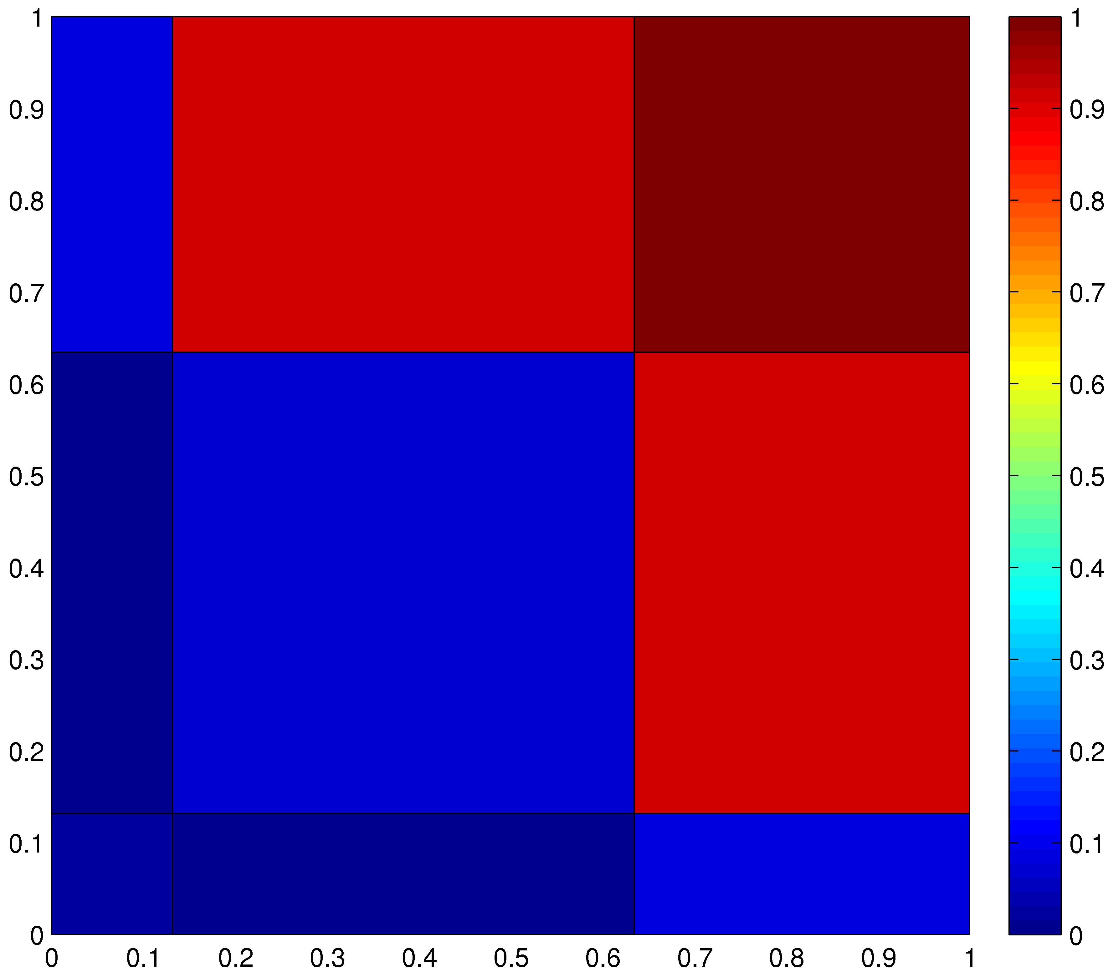
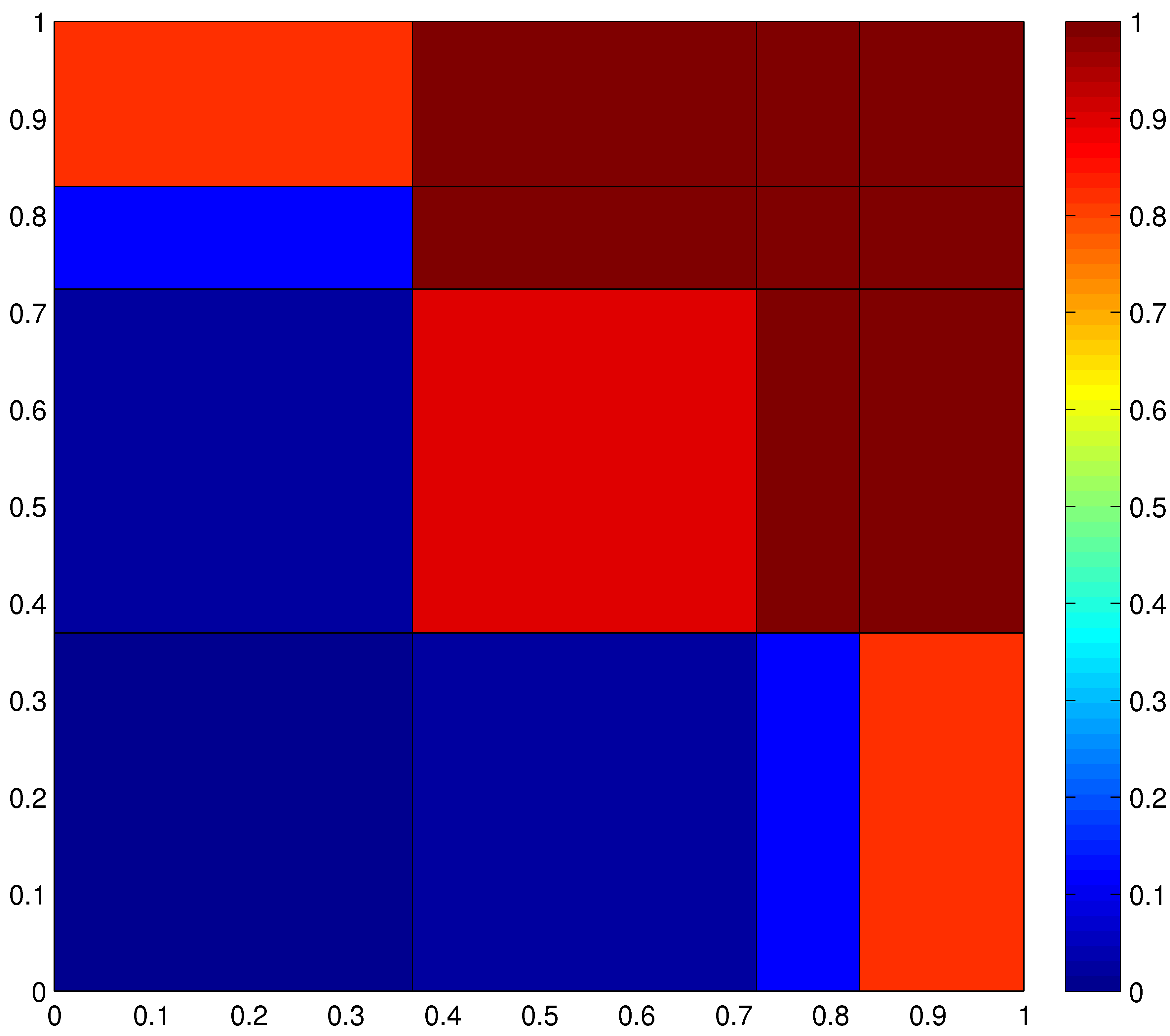
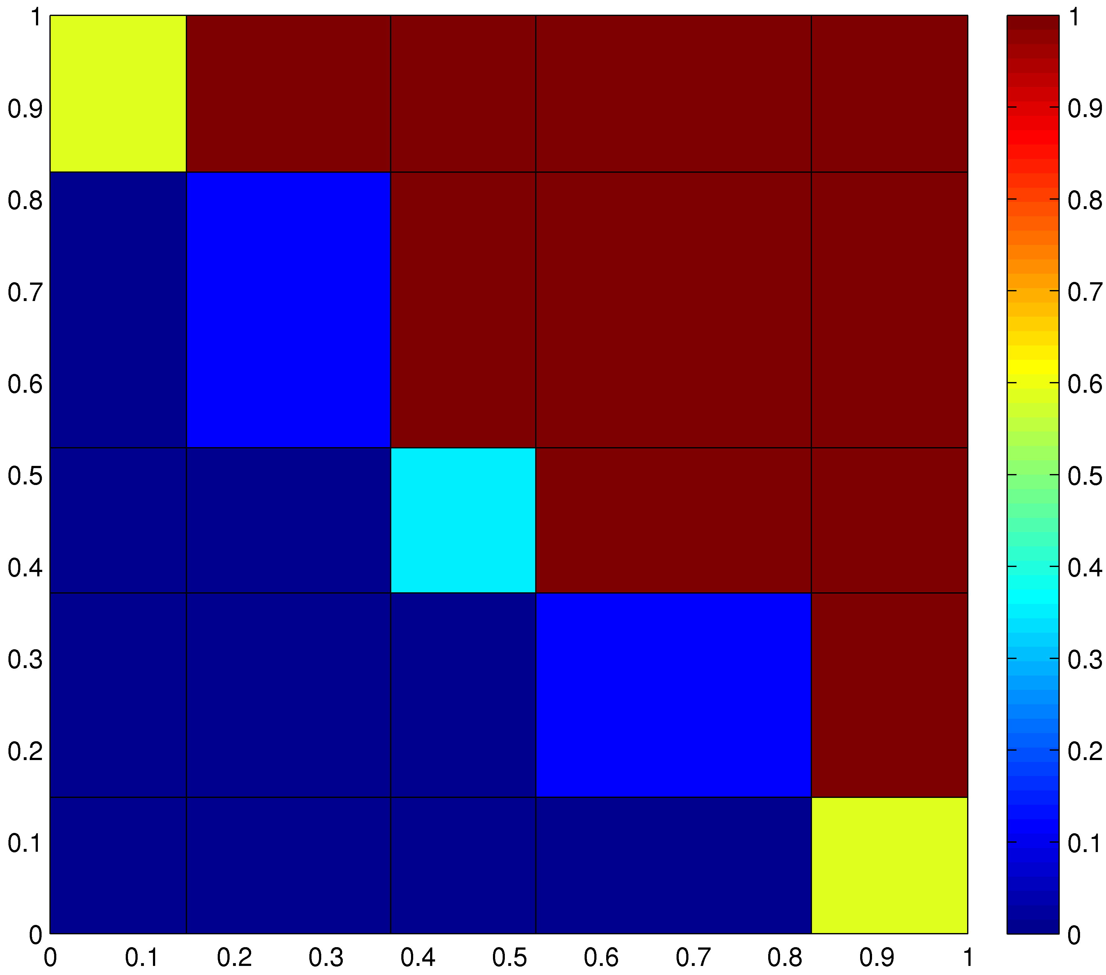
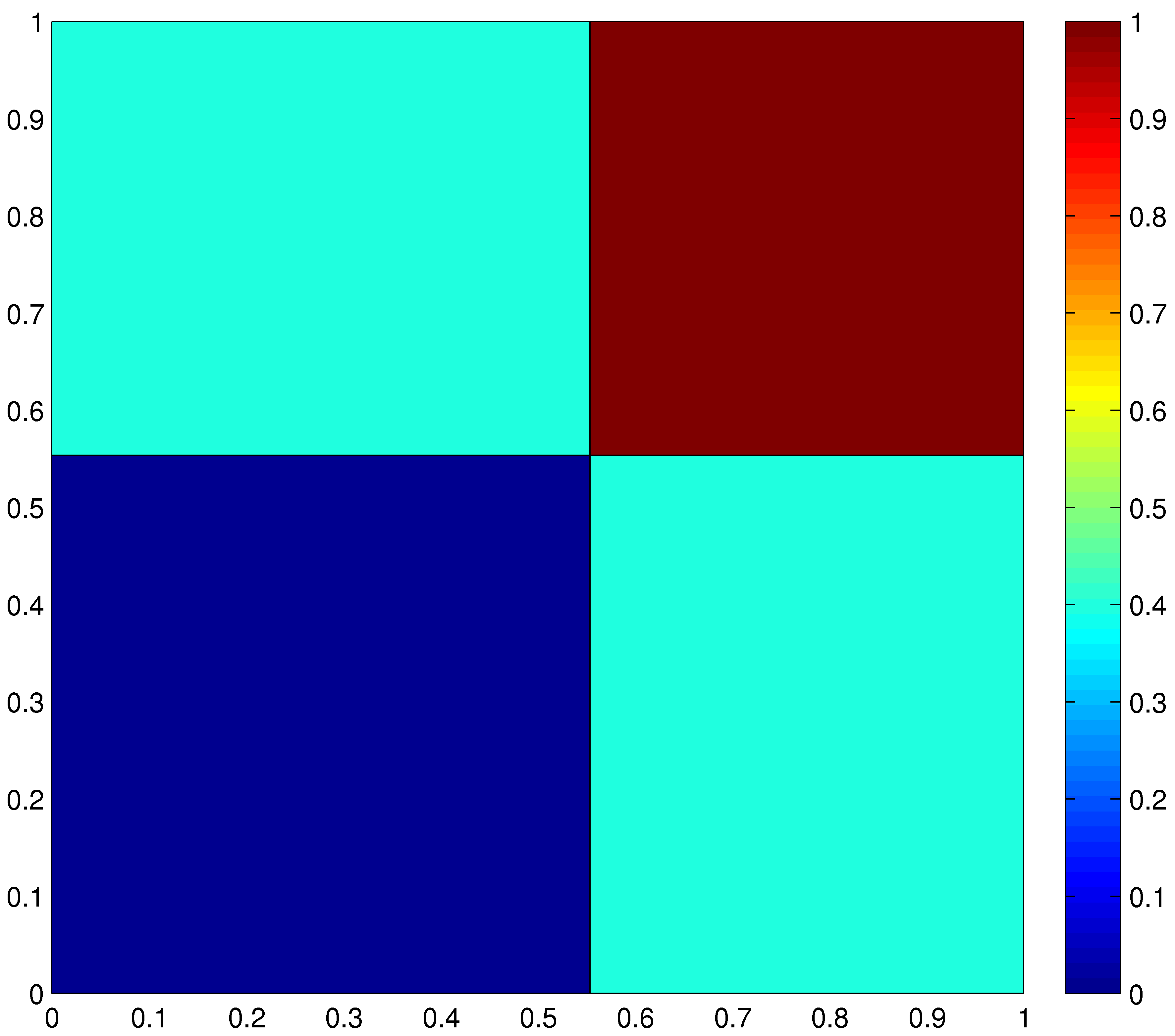
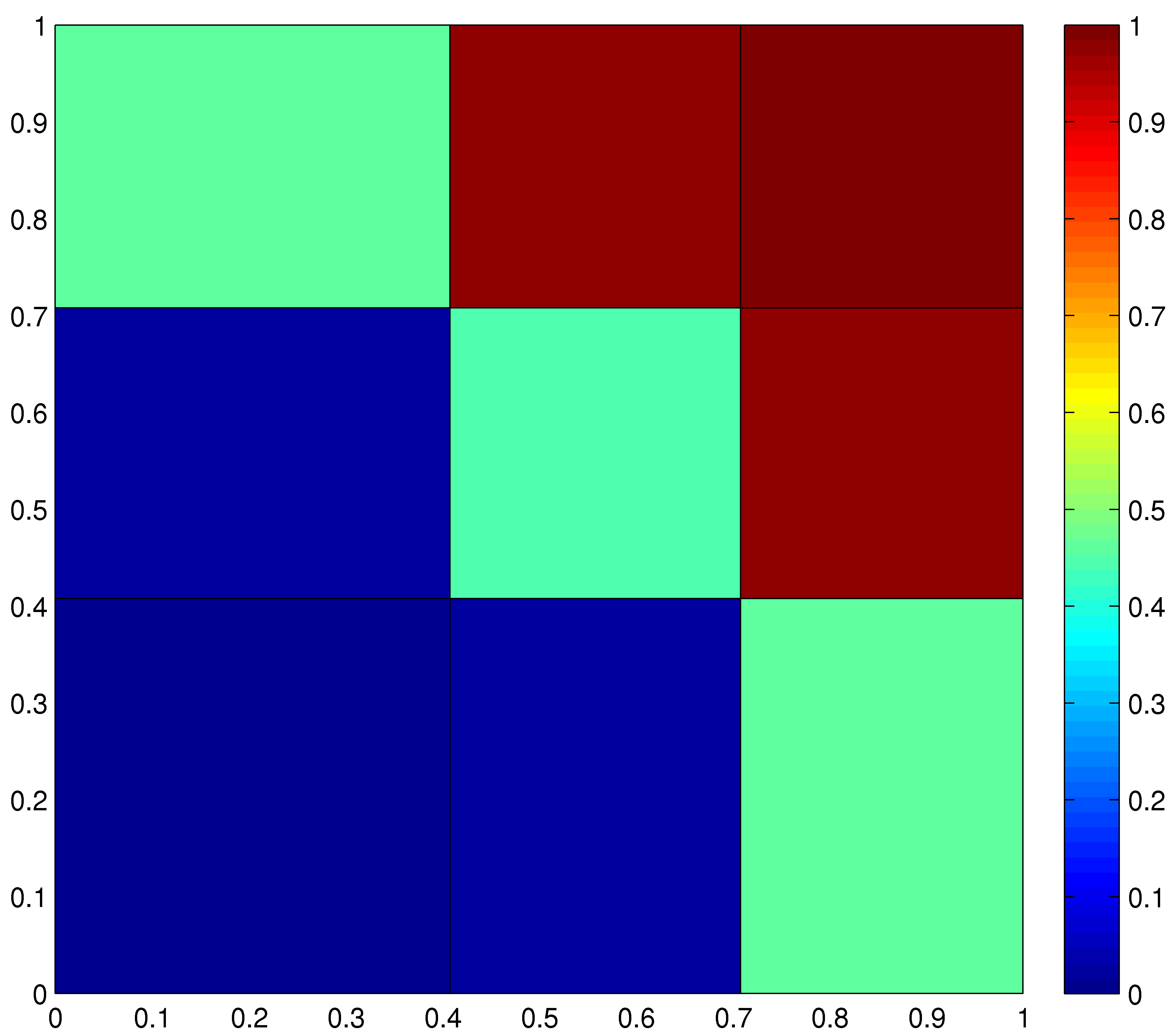
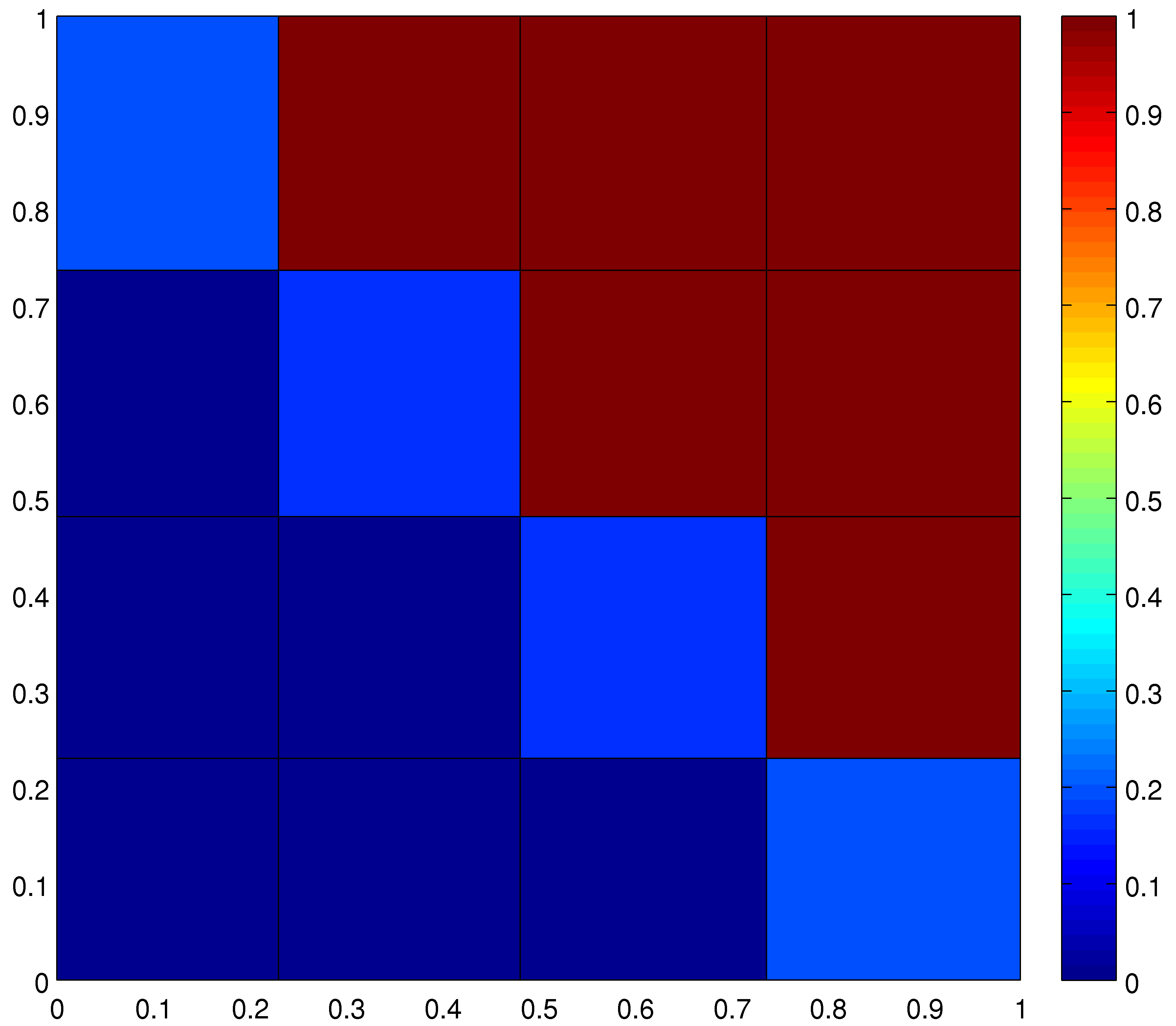
Figure 11: Maximizing graphons for the finitely forced model. Top row: maximizers with $(t_{1},t_{2},\tilde{t}_{3},\tilde{t}_{4})$ constraints at $\alpha=0.0200$ (left, 3-podal), $\alpha=0.0050$ (middle, 4-podal) and $\alpha=0.0015$ (right, 5-podal); Bottom row: maximizers with $(\zeta_{1},\zeta_{2})$ constraints at $\alpha=0.0200$ (left, 2-podal), $\alpha=0.0050$ (middle, 3-podal) and $\alpha=0.0015$ (right, 4-podal).

9 Conclusion

We first compare our results with exponential random graph models (ERGMs), also based on given subgraph densities; see [CD, RY, AR2, LZ, Y, YRF, AZ] for previous mathematical work on their asymptotics. For this we contrast the basic optimization problems underlying ERGMs and the models of this paper.

Intuitively the randomness in such random graph models arises, in modeling large networks, by starting with an assumption that a certain set of subgraphs $H=(H_{1},\ldots,H_{\ell})$ are ‘significant’ for the networks; one can then try to understand a large network as a ‘typical’ one for certain values $t_{H}(g)=(t_{H_{1}},\ldots,t_{H_{\ell}})$ of the densities $t_{H_{j}}$ of those subgraphs. Large deviations theory [CV] can then give probabilistic descriptions of such typical graphs through a variational principle for the constrained Shannon entropy, $s_{\tau}=\sup_{g|t_{H}(g)=\tau}\mathcal{S}(g)$.

In this paper, as in [RS1, RS2, RRS], we use such constrained optimization of entropy, and by analogy with statistical mechanics we call such models ‘microcanonical’. In contrast, ERGMs are analogues of ‘grand canonical’ models of statistical mechanics. As noted in Section 2, our microcanonical version consists of maximizing $\mathcal{S}(g)$ over graphons $g$ with fixed values $t_{H}(g)=\tau$, leading to a constrained-maximum entropy $s_{\tau}=\sup_{g|t_{H}(g)=\tau}\mathcal{S}(g)$. The optimizing graphons satisfy the Euler-Lagrange variational equation, $\delta[\mathcal{S}(g)+\beta\cdot t_{H}(g)]=0$, together with the constraints $t_{H}(g)=\tau$, for some set of Lagrange multipliers $\beta=(\beta_{1},\ldots,\beta_{\ell})$.

For the ERGM (grand canonical) approach, instead of fixing $t_{H}(g)$ one maximizes $\tilde{F}(g)=\mathcal{S}(g)+\beta\cdot t_{H}(g)$ for fixed $\beta$, obtaining

$$F_{\beta}=\sup_{g}\tilde{F}(g)=\sup_{g}[\mathcal{S}(g)+\beta\cdot t_{H}(g)].$$ (117)

It is typical for there to be a loss of information in the grand canonical modelling of large graphs. One way to see the loss is by comparing the parameter (“phase”) space $\Sigma_{mc}=\{\tau\}$ of the microcanonical model with that for the grand canonical model, $\Sigma_{gc}=\{\beta\}$. For each point $\beta$ of $\Sigma_{gc}$ there are optimizing graphons $\tilde{g}_{{}_{\beta}}$ such that $\tilde{F}(\tilde{g}_{{}_{\beta}})=F_{\beta}$, and for each point $\tau$ of $\Sigma_{mc}$ there are optimizing graphons $\tilde{g}_{\tau}$ such that $t_{H}(\tilde{g}_{\tau})=\tau$ and $\mathcal{S}(\tilde{g}_{\tau})=s_{\tau}$. Defining $\tau^{\prime}$ as $t_{H}(\tilde{g}_{{}_{\beta}})$ it follows that $\tilde{g}_{{}_{\beta}}$ maximizes $\mathcal{S}(g)$ under some constraint $\tau$, namely $\mathcal{S}(\tilde{g}_{{}_{\beta}})=s_{\tau^{\prime}}$. But the converse fails: there are some $\tau$ for which no optimizing $\tilde{g}_{{}_{\beta}}$ satisfies $t_{H}(\tilde{g}_{{}_{\beta}})=\tau$ [CD, RS1].

This asymmetry is particularly acute for the $k$-star models we discuss in this paper: it follows from [CD] that all of $\Sigma_{gc}$ is represented only on the lower boundary curve of $\Sigma_{mc}$, $\tau_{k}=\epsilon^{k}$: see Fig. 1. If one is interested in the influence of certain subgraph densities in a large network it is therefore preferable to use constrained optimization of entropy rather than to use the ERGM approach.

Finally, in trying to understand the ‘phase transition’ in the ERGM edge/triangle model it seems significant that the functional derivatives of the densities $\delta t/\delta g$ are linearly dependent at the optimizing (constant) graphons relevant to that transition. This was quite relevant in the perturbative analysis along the Erdős-Rényi curve in the microcanonical edge/triangle model [RS1]. And of course when the $\delta t/\delta g$ are linearly dependent they cannot play their usual role as coefficients in the expansion of the entropy $s_{\tau}$.

Next we consider the role of multipodal states in modeling large graphs. In [RS1, RS2, RRS] evidence, but not proof, of multipodal entropy optimizers was found throughout the phase space of the microcanonical edge/triangle model, and in this paper we have proven this to hold throughout the phase space of all $k$-star models. Consider more general microcanonical graph models with constraints on edge density, $e(g)$, and the densities $t_{H}(g)$ of a finite number of other subgraphs, $H$. We are interested in the generality of multipodality for entropy maximizing graphons in such models. As noted in the Introduction there are known examples (in some sense ‘rare’: see Theorem 7.12 in [LS3]) with nonmultipodality on phase space boundaries, but this is not known to occur in the interior of any phase space.

To pursue this we first note a superficial similarity between the subject of extremal graphs and the older subject of ‘densest packings of bodies’: Given a finite collection $\mathcal{C}$ of bodies $\{B_{1},\ldots,B_{\ell}\}$ in $\mathcal{R}^{d}$ determine those nonoverlapping arrangements, of unlimited numbers of congruent copies of the $B$’s, which maximize the fraction of $\mathcal{R}^{d}$ covered by the $B$’s. (See [Fej] for an overview.) As in extremal graph theory few examples have been solved, the main ones being congruent spheres for dimensions $d\leq 3$ and those bodies which can tile space, such as congruent regular hexagons in the plane. Based on this limited experience the assumption/expectation developed that for every collection $\mathcal{C}$ there would be a ‘crystalline’ densest packing, a packing whose symmetry group was small (cocompact) in the group of symmetries of $\mathcal{R}^{d}$. This assumption was proven incorrect in 1966 by the construction of ‘aperiodic tilings’; see [Sen, Ra] for an overview. One can therefore draw a parallel between aperiodic ‘counterexamples’ in the study of densest packings, and nonmultipodal ‘counterexamples’ in extremal graph theory. Using nonoverlapping bodies to model molecules, physicists have applied the formalism of statistical mechanics to packings of bodies. Packings of spheres then give rise to the ‘hard sphere model’ which is a simple model for which simulation (not proof) shows the emergence of a crystalline phase in the interior of the phase space [Low]. More recently, aperiodic tilings have been used to model quasicrystalline phases of matter. (See [J] for an introductory guide to quasicrystals.) Although it is expected that the tilings, corresponding to optimal density on the boundary of the microcanonical phase space, give rise to an emergent quasicrystalline phase in the interior, there is much less simulation evidence of this, as yet, than for crystalline phases emerging from crystalline sphere packings; see [AR1] and references therein.

Getting back to networks we note that simple constraints give rise to multipodal optimal graphs on the boundary of the phase space, and also [RS1, RS2, RRS] multipodal phases in the interior, in parallel to the crystalline situation in packing. By analogy with packing therefore, a natural question is: do the nonmultipodal ‘counterexamples’ on the phase space boundary of random graph models give rise to nonmultipodal phases in the interior of the phase space, in parallel to aperiodic tilings and quasicrystalline phases? (As in statistical mechanics a phase is defined as a connected open subset of the phase space of the model, in which the entropy is analytic; see [RS1].)

Question 1. Are random graph phases always multipodal?

Our attempt to investigate this in Section 8 was inconclusive.

Multipodality is a useful tool in understanding phases. For instance in the edge/triangle model [RS1, RS2, RRS] even a cursory inspection of the largest values of such an optimizing graphon concentrates attention on the conditions under which edges tend to clump together (fluid-like behavior) or push apart into segregated patterns (solid-like behavior). More specifically, we note that in simulations of the edge/triangle model [RRS] it is very noticeable that at densities above the Erdős-Rényi curve the optimizing graphons are always monotone, while this is rarely if ever the case below the curve. We proved in this paper that in $k$-star models, for which densities are always above the ER curve, the optimizing graphons are always monotone. Consider a general model with two densities, edges and some graph $H$. The ER curve is $\tau_{H}=\epsilon^{k}$ where $k$ is the number of edges in $H$. A natural question is:

Question 2. Are the optimizing graphons always monotone above the ER curve in such random graph models?

In equilibrium statistical mechanics [Ru] one can rarely understand directly the equilibrium distribution in a useful way, at least away from extreme values of energy or pressure, so one determines the basic characteristics of a model by estimating order parameters or other secondary quantities. In random graph models multipodal structure of the optimizing state gives hope for a more direct understanding of the emergent properties of a model. This would be a significant shift of viewpoint.

References

- [AK] R. Ahlswede and G.O.H. Katona, Graphs with maximal number of adjacent pairs of edges, Acta Math. Acad. Sci. Hungar. 32 (1978) 97-120
- [AR1] D. Aristoff and C. Radin, First order phase transition in a model of quasicrystals, J. Phys. A: Math. Theor. 44(2011), 255001.
- [AR2] D. Aristoff and C. Radin, Emergent structures in large networks, J. Appl. Probab. 50 (2013) 883-888.
- [AZ] D. Aristoff and L. Zhu, On the phase transition curve in a directed exponential random graph model, arxiv:1404.6514
- [B] B. Bollobas, Extremal graph theory, Dover Publications, New York, 2004.
- [BCL] C. Borgs, J. Chayes and L. Lovász, Moments of two-variable functions and the uniqueness of graph limits, Geom. Funct. Anal. 19 (2010) 1597-1619.
- [BCLSV] C. Borgs, J. Chayes, L. Lovász, V.T. Sós and K. Vesztergombi, Convergent graph sequences I: subgraph frequencies, metric properties, and testing, Adv. Math. 219 (2008) 1801-1851.
- [CD] S. Chatterjee and P. Diaconis, Estimating and understanding exponential random graph models, Ann. Statist. 41 (2013) 2428-2461.
- [CDS] S. Chatterjee, P. Diaconis and A. Sly, Random graphs with a given degree sequence, Ann. Appl. Probab. 21 (2011) 1400-1435.
- [CV] S. Chatterjee and S.R.S. Varadhan, The large deviation principle for the Erdős-Rényi random graph, Eur. J. Comb. 32 (2011) 1000-1017.
- [Fej] L. Fejes Tóth, Regular Figures, Macmillan, New York, 1964.
- [J] C. Janot, Quasicrystals: A primer, Oxford University Press, Oxford, 1997.
- [Lov] L. Lovász, Large networks and graph limits, American Mathematical Society, Providence, 2012.
- [Low] H. Löwen, Fun with hard spheres, In: “Spatial Statistics and Statistical Physics”, edited by K. Mecke and D. Stoyan, Springer Lecture Notes in Physics, volume 554, pages 295–331, Berlin, 2000.
- [LS1] L. Lovász and B. Szegedy, Limits of dense graph sequences, J. Combin. Theory Ser. B 98 (2006) 933-957.
- [LS2] L. Lovász and B. Szegedy, Szemerédi’s lemma for the analyst, GAFA 17 (2007) 252-270.
- [LS3] L. Lovász and B. Szegedy, Finitely forcible graphons, J. Combin. Theory Ser. B 101 (2011) 269-301.
- [LZ] E. Lubetzky and Y. Zhao, On replica symmetry of large deviations in random graphs, Random Structures and Algorithms 47 (2015) 109–146.
- [N] M.E.J. Newman, Networks: an Introduction, Oxford University Press, 2010.
- [P] O. Pikhurko, private communication.
- [R] C. Reiher, The clique density theorem, Ann. Math. (to appear), arXiv:1212.2454.
- [Ra] C. Radin, Miles of Tiles, Student Mathematical Library, Vol 1, Amer. Math. Soc., Providence, 1999.
- [RRS] C. Radin, K. Ren and L. Sadun, The asymptotics of large constrained graphs, J. Phys. A: Math. Theor. 47 (2014) 175001.
- [RS1] C. Radin and L. Sadun, Phase transitions in a complex network, J. Phys. A: Math. Theor. 46 (2013) 305002.
- [RS2] C. Radin and L. Sadun, Singularities in the entropy of asymptotically large simple graphs, J. Stat. Phys. 158 (2015) 853–865.
- [Ru] D. Ruelle Statistical Mechanics; Rigorous Results, Benjamin, New York, 1969.
- [RY] C. Radin and M. Yin, Phase transitions in exponential random graphs, Ann. Appl. Probab. 23 (2013) 2458-2471.
- [Sen] M. Senechal, Quasicrystals and geometry, Cambridge University Press, Cambridge, 1995.
- [TET] H. Touchette, R.S. Ellis and B. Turkington, Physica A 340 (2004) 138-146.
- [Y] M. Yin, Critical phenomena in exponential random graphs, J. Stat. Phys. 153 (2013) 1008-1021.
- [YRF] M. Yin, A. Rinaldo and S. Fadnavis, Asymptotic quantization of exponential random graphs, Ann. Appl. Probab. (to appear), arXiv:1311.1738 (2013).