Force fluctuations in stretching a tethered polymer

Abstract

The recently proposed fluctuation relation in unfolding forces [Phys. Rev. E 84, 060101(R) (2011)] is re-examined taking into account the explicit time dependence of the force distribution. The stretching of a tethered Rouse polymer is exactly solved and the ratio of the probabilities of positive to negative forces is shown to be an exponential in force. Extensive steered molecular dynamics simulations of unfolding of deca alanine peptide confirm the form of fluctuation relation proposed earlier, but with explicit correct time dependence of unfolding forces taken into account. From exact calculations and simulations, a linear dependence of the constant in the exponential of the fluctuation relation on average unfolding forces and inverse temperature is proposed.

I Introduction

Fluctuation theorems provide a mechanism for characterizing fluctuations in non-equilibrium processes Bustamante et al. (2005); Evans et al. (2002); Jarzynski (2008); Sevick et al. (2008); Jarzynski (2011). These fluctuations become increasingly relevant as the system size becomes smaller. Many biological systems are nano-sized and have inherently non-equilibrium processes. Fluctuation theorems have been realized in single molecule experiments such as dragging of a colloidal particle in an optical trap Wang et al. (2002͒); Trepagnier et al. (2004), RNA unfolding experiments Liphardt et al. (2002); Collin et al. (2005), and mechanical unfolding of proteins Shank et al. (2010); Imparato et al. (2008).

Non-equilibrium transient and steady states follow transient Evans and Searles (1994); Evans et al. (2002); Van Zon and Cohen (2003); Chakrabarti (2009) (TFT) and steady state (SSFT) Evans et al. (1993); Gallavotti and Cohen (1995); Searles and Evans (1999); Bonetto and Lebowitz (2001); Zamponi et al. (2004); Belushkin et al. (2011) fluctuation theorems respectively. In this paper, we are concerned with TFT-like relation in unfolding forces of a tethered polymer. In TFT, the system is initially in an equilibrium state and fluctuations of quantities such as entropy, work, power flux and heat absorbed are measured over an arbitrary time interval Wang et al. (2002͒); Feitosa and Menon (2004͒); van Zon and Cohen (2003); Aumatre et al. (2001); van Zon et al. (2004); Goldburg et al. (2001). For instance, the transient work fluctuation theorem Evans and Searles (1994); Kurchan (2007) has the form $P(W)/P(-W)=e^{\beta W}$, where $P(W)$ is the probability of work $W$ being done on the system. The Jarzynski’s relation Jarzynski (1997), which relates the equilibrium free energy to non-equilibrium work, is a special form of transient work fluctuation theorem, when the initial and final states are equilibrium states.

More recently, fluctuation theorems of non-traditional thermodynamic variables like reaction coordinates Paramore et al. (2007a, b) and unfolding forces Ponmurugan and Vemparala (2011) have been studied. In Ref. Ponmurugan and Vemparala (2011), based on constant velocity steered molecular dynamics (SMD) simulations of unfolding of contactin1 protein and deca alanine peptide, a fluctuation relation of the form

$$\frac{P_{v}(+f)}{P_{v}(-f)}=\exp\left[\Gamma(T,v)f\right],$$ (1)

was proposed, where, $v$ is the unfolding velocity and $f$ is the unfolding force at constant temperature $T$. The constant $\Gamma(T,v)$ was observed to have the scaling form

$$\Gamma(T,v)\sim v^{\alpha}T^{-\delta}.$$ (2)

For contactin1 protein $\alpha\approx 0.15$ and $\delta\approx 0.7$ and for deca alanine $\alpha\approx 0.03$ and $\delta\approx 3.8$ Ponmurugan and Vemparala (2011). However, analytical calculations for a Brownian particle in a harmonic oscillator, moving at a constant velocity, show that though the form of the fluctuation relation as proposed in Ref. Ponmurugan and Vemparala (2011) is retained, the exponents $\alpha$ and $\delta$ are equal to $1$ Minh (2012); Sharma and Cherayil (2012). It is to be noted that while the SMD simulations Ponmurugan and Vemparala (2011) were for a tethered molecule, the calculations Minh (2012); Sharma and Cherayil (2012) are for a non-tethered particle. For a tethered molecule, the unfolding process is non-stationary and the fluctuation relation, if it exists, should include an explicit time dependence. To address this issue, in this paper, we solve exactly the time dependent force distribution $P_{v}(f,t)$ for a Rouse polymer and show that $P_{v}(f,t)$ is Gaussian and hence follows a fluctuation relation

$$\frac{P_{v}(+f,t)}{P_{v}(-f,t)}=\exp\left[\Gamma\left(T,\langle f(t)\rangle\right)f\right],$$ (3)

with

$$\Gamma(T,\langle f(t)\rangle)=\frac{2\langle f(t)\rangle}{\alpha^{\prime}T},$$ (4)

where $\langle f(t)\rangle$ is the time dependent average force and $\alpha^{\prime}$ is a system dependent constant. In case of Rouse polymer, the time dependent average force is linear in extension and hence unfolding velocity. We then perform extensive SMD simulations of deca alanine in vacuum and show that, though the system has non-linear force-extension relation, the data for force distribution is still consistent with Eq. (3).

II Force distribution while stretching a rouse polymer

In this section, we solve for the time dependent force distribution in a tethered Rouse polymer. We closely follow the solution for the work distribution derived in Ref. Dhar (2005). Consider a one dimensional Gaussian chain consisting of $N+2$ particles. The particles are connected to each other by harmonic springs such that the Hamiltonian of the system is

$$H=\frac{k}{2}\sum_{i=1}^{N+1}\left(x_{i}-x_{i-1}\right)^{2},$$ (5)

where $x_{i}$ is the position of the $i^{\text{th}}$ particle, and $k$ is a constant. The first particle is held fixed at the origin and the last particle is pulled with a constant velocity $v$, i.e., $x_{0}(t)=0$, and $x_{N+1}(t)=x_{N+1}(0)+vt$. We assume Rouse dynamics, where the over damped Langevin equation for the chain is given by

$$\frac{dx_{i}}{dt}=-\frac{k}{\gamma}(2x_{i}-x_{i+1}-x_{i-1})+\eta_{i}(t),~{}i=1,2,\ldots N,$$ (6)

where $\gamma$ is the friction coefficient and $\eta$ is white Gaussian noise with $\langle\eta_{i}(t)\rangle=0$ and $\langle\eta_{i}(t)\eta_{j}(t^{\prime})\rangle=\frac{2}{\beta\gamma}\delta(t-t^{\prime})$, where $\beta$ is the inverse temperature. For convenience, we set $\gamma=1$. It can be recovered in the later expressions by letting $k\rightarrow k/\gamma$ and $\beta\rightarrow\beta\gamma$. Equation (6) may be written in matrix notation as

$$\frac{d{\bf x}}{dt}=-{\bf A}{\bf x}+{\bf h}(t)+{\bf\eta}(t).$$ (7)

where ${\bf x}=(x_{1},...,x_{N})^{T}$, ${\bf\eta}=(\eta_{1},...,\eta_{N})^{T}$, and ${\bf h}=(0,...,h_{N})^{T}$, $h_{N}$ being $k\left[x_{N+1}(0)+vt\right]$. A is a tridiagonal symmetric matrix with non-zero entries $A_{i,i}=2k$, $A_{i,i+1}=A_{i,i-1}=-k$.

${\bf A}$ is diagonalized by an orthogonal transformation ${\bf O}^{T}{\bf AO}={\bf\Lambda}$, where ${\bf O}^{T}$ = ${\bf O}^{-1}$ and ${\bf\Lambda}$ is diagonal with $\Lambda_{mn}=\lambda_{m}\delta_{mn}$, where $\lambda_{m}$’s are the eigenvalues of ${\bf A}$. The eigenvalues $\lambda_{m}$ of ${\bf A}$, and the orthogonal matrix ${\bf O}$ are given by Mehta (1989)

$$\lambda_{m} = 2k\left[1-\cos\left(\frac{m\pi}{N+1}\right)\right],$$ (8)

$$O_{mn} = \sqrt{\frac{2}{N+1}}\sin\left(\frac{mn\pi}{N+1}\right).$$ (9)

Multiplying Eq. (7) with ${\bf O}^{T}$, we obtain

$$\frac{d\tilde{\bf x}}{dt}=-{\bf\Lambda}\tilde{\bf x}+\tilde{\bf h}+\tilde{\bf\eta},$$ (10)

where $\tilde{\bf x}={\bf O}^{T}{\bf x}$, $\tilde{\bf h}={\bf O}^{T}{\bf h}$ and $\tilde{\bf\eta}={\bf O}^{T}{\bf\eta}$. The general solution of Eq. (10) is

$$\tilde{\bf x}(t)=e^{-{\bf\Lambda}t}\tilde{\bf x}(0)+\int_{0}^{t}dt^{\prime}e^{-{\bf\Lambda}(t-t^{\prime})}\left[\tilde{\bf h}(t^{\prime})+\tilde{\bf\eta}(t^{\prime})\right].$$ (11)

The positions ${\bf x}(t)$ can be obtained from $\tilde{\bf x}(t)$ by ${\bf x}={\bf O}\tilde{\bf x}$. Since all the eigenvalues of the matrix ${\bf A}$ are positive [see Eq. (8)], the first term in Eq. (11) does not contribute in the limit of large time and for convenience we set $\tilde{\bf x}(0)={\bf 0}$. Then, the position of the $N^{\text{th}}$ particle is given by

$$x_{N}(t)=\sum_{m=1}^{N}O_{Nm}\int_{0}^{t}dt_{1}e^{-\lambda_{m}(t-t_{1})}\left[\tilde{h}_{m}(t_{1})+\tilde{\eta}_{m}(t_{1})\right].$$ (12)

The stretching force in the spring connecting the $N^{\text{th}}$ and the $(N+1)^{\text{th}}$ particle is given by $f(t)=k\left[x_{N+1}(t)-x_{N}(t)\right]=k\left[vt-x_{N}(t)\right]$. From Eq. (12) we see that $x_{N}$ is linear in the white noise $\eta$ and therefore its probability distribution function will be a Gaussian. Likewise, $P_{v}(f,t$), the distribution for force will be a Gaussian with $\langle f\rangle=k\left[vt-\langle x_{N}(t)\rangle\right]$ and $\langle f^{2}\rangle-\langle f\rangle^{2}=k^{2}[\langle x_{N}^{2}\rangle-\langle x_{N}\rangle^{2}]$. We have to compute only the first two moments of $x_{N}(t)$.

Averaging over noise in Eq. (12), and using $\tilde{h}_{m}=kvtO_{Nm}$, we obtain

$$\langle x_{N}(t)\rangle=\sum_{m=1}^{N}O_{Nm}^{2}\frac{kv}{\lambda_{m}}\left[t-\frac{1-e^{-\lambda_{m}t}}{\lambda_{m}}\right],$$ (13)

and

$$\langle x_{N}^{2}(t)\rangle-\langle x_{N}(t)\rangle^{2}=\frac{1}{\beta}\sum_{m=1}^{N}O_{Nm}^{2}\frac{1-e^{-2\lambda_{m}t}}{\lambda_{m}}.$$ (14)

The results simplify in the limit of large time, when the exponential terms in Eq. (13) and Eq. (14) can be dropped. Then,

$$\langle x_{N}(t)\rangle = vt\alpha_{1}-\frac{v}{k}\alpha_{2},$$ (15)

$$\langle x_{N}^{2}(t)\rangle-\langle x_{N}(t)\rangle^{2} = \frac{T}{k}\alpha_{1},$$ (16)

where

$$\alpha_{1} = k\sum_{m=1}^{N}\frac{O_{Nm}^{2}}{\lambda_{m}}$$ (17)

$$= \frac{1}{N+1}\sum_{m=1}^{N}\frac{\sin^{2}\left(\frac{N\pi}{N+1}m\right)}{\left[1-\cos\left(\frac{m\pi}{N+1}\right)\right]},$$

and

$$\alpha_{2} = k^{2}\sum_{m=1}^{N}\frac{O_{Nm}^{2}}{\lambda_{m}^{2}}$$ (18)

$$= \frac{1}{2\left(N+1\right)}\sum_{m=1}^{N}\frac{\sin^{2}\left(\frac{N\pi}{N+1}m\right)}{\left[1-\cos\left(\frac{m\pi}{N+1}\right)\right]^{2}},$$

are constants which depend only on $N$. Rewriting in terms of force, we obtain

$$\langle f\rangle = kvt[1-\alpha_{1}]+v\alpha_{2},$$ (19)

$$\sigma^{2} = \langle f^{2}\rangle-\langle f\rangle^{2}=kT\alpha_{1}.$$ (20)

The force is then distributed as

$$P_{v}(f,t)=\frac{1}{\left(2\pi kT\alpha_{1}\right)^{1/2}}\exp\left[-\frac{\left(f-\langle f\rangle\right)^{2}}{2kT\alpha_{1}}\right],$$ (21)

with $\langle f\rangle$ as in Eq. (19). Clearly,

$$\ln\left[\frac{P_{v}(+f,t)}{P_{v}(-f,t)}\right]=\frac{2f\langle f\rangle}{kT\alpha_{1}},$$ (22)

where the unfolding velocity $v$ is absorbed into $\langle f\rangle$ through Eq. (19). For the Rouse model considered here, $\langle f\rangle\propto v$, and hence Eq. (22) has the same form as the fluctuation relation Eq. (1) with $\alpha=1$ and $\delta=1$, identical to the results obtained for a Brownian particle in a harmonic oscillator Minh (2012); Sharma and Cherayil (2012). However, if the dependence of $\langle f\rangle$ on $v$ is more complicated, then the exponent in unfolding velocity, $\alpha$, may not be well defined.

We now do a numerical validation of the solution. We numerically solve Rouse model by integrating the equations of motion, Eq (6), with initial condition $x_{i}(0)=0$ for all $i$. The force $f$ is then obtained by $f=k(vt-x_{N})$. In Fig. 1 we show the data collapse of $\ln[P_{v}(+f,t)/P_{v}(-f,t)]$ for various values of $v$ and $T$, when scaled as in Eq. (22) with $\langle f\rangle\sim v$. The agreement between the numerical and exact solutions is excellent.

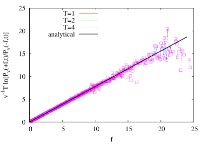
Figure 1: (Color online) The ratio $\ln[P_{v}(+f,t)/P_{v}(-f,t)]$ for different temperatures and unfolding velocities for the Rouse model collapse onto a single curve when scaled as in Eq. (22). The data are for $T=1,2$ and $4$. The unfolding velocities are $1.0$ ($\Box$), $2.0$ ($\circ$) and $4.0$ ($\triangle$). The data points are averaged over $3\times 10^{6}$ realizations.

Now, we would like to confirm whether Eq. (22) holds for a more realistic polymer. For contactin1 protein simulations done in Ref. Ponmurugan and Vemparala (2011), the prohibitive computational time due to presence of large number of solvent molecules limited the number of SMD runs from $3$–$30$. Obtaining reliable time dependent $P_{v}(f,t)$ from such limited data set is not possible. On the other hand, deca alanine in vacuum is a good test system that is computationally inexpensive. In the next section, we describe set up and results of extensive SMD runs for deca alanine.

III Steered MD simulations of deca alanine

In this section, we describe the results of SMD simulations on deca alanine molecule, a prototypical system that has been used earlier for demonstrating calculation of potential of mean force using Jarzynski’s relation Park et al. (2003); Park and Schulten (2004); Oer et al. (2012) and adaptive bias force methods Henin and Chipot (2004); Chipot and Henin (2005). Deca alanine molecule adopts a helical conformation in vacuum and the SMD simulations have been performed by fixing the C-terminal C$\alpha$ atom and unfolding the molecule by pulling the N-terminal C$\alpha$ atom along the helical axis with a constant velocity. SMD simulations were performed at three different temperatures using three different unfolding velocities (details of simulation setup are given in Table 1). For each of the parameter sets, 1000 SMD simulations were performed. Deca alanine was equilibrated for 10 ns in vacuum in constant temperature-volume (NVT) conditions and from the last 5 ns of the run, the initial configurations for the SMD simulations were generated by extracting 1000 snap shots. All the equilibrium and SMD simulations were performed by NAMD (version 2.7b3) Phillips et al. (2005) using the CHARMM22 force field supplemented by CMAP corrections Buck et al. (2006) for deca alanine. A cutoff of $12$Åwas used for van der Waals interactions and particle mesh Ewald method was used to handle long range electrostatics interactions. Langevin dynamics were used for temperature control and the box size was chosen to be large enough to accommodate the stretched deca alanine molecule and to avoid interactions with the periodic images. A spring constant of 10 Kcal/mol/Ų was used for all the SMD runs.

Table 1: SMD simulation details of unfolding deca alanine for different unfolding velocities $v$ and temperatures $T$ for spring constant $K=10$ Kcal/mol/Ų.

$v$	$T$	number of
(Å/ps)	(K)	SMD runs
0.05	300	1000
0.1	300	1000
0.1	250	1000
0.1	150	1000
0.2	300	1000

To construct $P_{v}(f,t)$, we consider all the unfolding forces in a time window $(t-\Delta,t+\Delta)$ and average over $1000$ SMD runs, where an optimum value of $\Delta$ is chosen such that we obtain good statistics that are independent of $\Delta$. In Fig. 2, we show that the data for different temperatures and times, for the same unfolding velocity, collapse on to one curve when scaled as in Eq. (22). Likewise, we find good collapse for data for different unfolding velocities and same temperature (see Fig. 3).

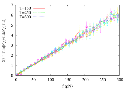
Figure 2: (Color online) The ratio $\ln[P_{v}(+f,t)/P_{v}(-f,t)]$ for different extensions and temperatures for deca alanine collapse onto a single curve when scaled as in Eq. (22). The data are for $T=150,250$ and $300K$. The extensions are $2$Å($\Box$), $4$Å($\circ$) and $7$Å($\triangle$). All data are for unfolding velocity $v=0.1$Å/ps.

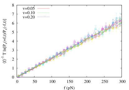
Figure 3: (Color online) The ratio $\ln[P_{v}(+f,t)/P_{v}(-f,t)]$ for different extensions and unfolding velocities for deca alanine collapse onto a single curve when scaled as in Eq. (22). The data are for $v=0.05,0.10$ and $0.20$Å/ps. The extensions are $2$Å($\Box$), $4$Å($\circ$) and $7$Å($\triangle$). All data are for temperature $T=300K$.

It is to be noted that for the collapse in Figs. 2 and 3, we scaled the ratio of probabilities by the mean force $\langle f\rangle$ rather than by $v$ as in Fig. 1. The average force $\langle f\rangle$ for deca alanine is not a simple linear function of the extension $vt$ (see Fig. 4). Therefore, $\alpha$ [see Eq. (2] is ill-defined for deca alanine, though $\delta$ is seen to be $1$. From the exact calculations and simulations, we expect that Eq. (4) rather than Eq. (2) will hold for the stretching of a generic molecule.

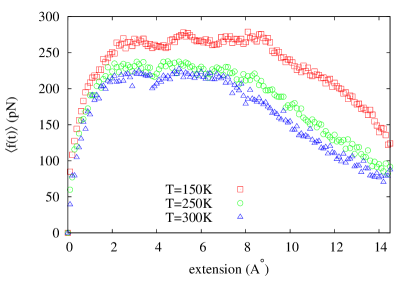
Figure 4: (Color online) The average force as a function of extension for different temperatures and fixed unfolding velocity $v=0.10$Å/ps for deca alanine .

IV Conclusion

In this paper, we re-examine the recently proposed fluctuation relation, Eqs. (1) and (2), in unfolding forces observed in the SMD simulations of single molecules Ponmurugan and Vemparala (2011). Here, we include the essential time dependence into the force distributions, which was ignored in Ref. Ponmurugan and Vemparala (2011). First, we solved exactly the time dependent force distribution for a tethered Rouse polymer that is being unfolded at constant velocity. For this system, we obtain the fluctuation relation Eq. (3) which has the same form as Eq. (1) when the average unfolding force is proportional to the unfolding velocity as is the case in the Rouse model. Second, using extensive SMD simulations of deca alanine peptide in vacuum for varying temperatures and unfolding velocities, we show that the data are consistent with the fluctuation relation as in Eq. (3) even though the average unfolding force is not a simple function of unfolding velocity. The constant $\Gamma$ defined in Eq. (1) was proposed to be of the form $v^{\alpha}T^{-\delta}$ Ponmurugan and Vemparala (2011). Rather, we find $\Gamma\propto\langle f\rangle T^{-1}$ as in Eq. (4), where $\langle f\rangle$ is a system dependent function of the unfolding velocity. It reduces to the form $vT^{-1}$ for simple cases of a Brownian particle in a harmonic potential  Minh (2012); Sharma and Cherayil (2012) or the Rouse model considered here.

If the time dependent force distribution is Gaussian, then the fluctuation relation will have the form Eqs. (3) and (22). In this paper, we showed that for a Rouse polymer the force distribution is indeed Gaussian. A priori, there is no obvious reason to expect Gaussian distribution for a more realistic polymer. However, for the prototypical deca alanine peptide studied here, the force distribution appears to be Gaussian throughout the range of unfolding forces considered and also at various times along the unfolding trajectory making it plausible that the force distribution is Gaussian for an arbitrary molecule.

The proposed fluctuation relation in Ref  Ponmurugan and Vemparala (2011) and its time dependent form in this paper, augment the list of fluctuation relations (albeit in more conventional variables) in the literature. This may be realized in the single molecule unfolding experiments.

References

- Bustamante et al. (2005) C. Bustamante, J. Liphardt, and F. Ritort, Phys. Today 58, 43 (2005).
- Evans et al. (2002) D. J. Evans, E. G. D. Cohen, and G. P. Morriss, Adv. Phys. 51, 1529 (2002).
- Jarzynski (2008) C. Jarzynski, Eur. Phys. J. B 64, 331 (2008).
- Sevick et al. (2008) E. Sevick, R. Prabhakar, S. R. Williams, and D. J. Searles, Annu. Rev. Phys. Chem. 59, 603 (2008).
- Jarzynski (2011) C. Jarzynski, Annu. Rev. Condense. Matter Phys. 2, 329 (2011).
- Wang et al. (2002͒) G. M. Wang, E. M. Sevick, E. Mittag, D. J. Searles, and D. J. Evans, Phys. Rev. Lett. 89, 050601 (2002͒).
- Trepagnier et al. (2004) E. H. Trepagnier, C. Jarzynski, F. Ritort, G. E. Crooks, C. Bustamante, and J. Liphardt, Proc. Nat. Acad. Sci. 101, 15038–15041 (2004).
- Liphardt et al. (2002) J. Liphardt, S. Dumont, S. B. Smith, I. Tinoco, and C. Bustamante, Science 296, 1832 (2002).
- Collin et al. (2005) D. Collin, F. Ritort, C. Jarzynski, S. B. Smith, I. T. Jr., and C. Bustamante, Nature 437, 231–234 (2005).
- Shank et al. (2010) E. A. Shank, C. Cecconi, J. W. Dill, S. Marqusee, and C. Bustamante, Nature 465, 637 (2010).
- Imparato et al. (2008) A. Imparato, F. Sbrana, and M. Vassalli, Europhys. Lett. 82, 58006 (2008).
- Evans and Searles (1994) D. J. Evans and D. J. Searles, Phys. Rev. E 50, 1645 (1994).
- Van Zon and Cohen (2003) R. Van Zon and E. G. D. Cohen, Phys. Rev. E 67, 046102 (2003).
- Chakrabarti (2009) R. Chakrabarti, Pramana 72, 665 (2009).
- Evans et al. (1993) D. J. Evans, E. G. D. Cohen, and G. P. Morriss, Phys. Rev. Lett. 71, 2401 (1993).
- Gallavotti and Cohen (1995) G. Gallavotti and E. G. D. Cohen, Phys. Rev. Lett. 74, 2694 (1995).
- Searles and Evans (1999) D. J. Searles and D. J. Evans, Phys. Rev. E 60, 159 (1999).
- Bonetto and Lebowitz (2001) F. Bonetto and J. L. Lebowitz, Phys. Rev. E 64, 056129 (2001).
- Zamponi et al. (2004) F. Zamponi, G. Ruocco, and L. Angelani, J. Stat. Phys. 115, 1655 (2004).
- Belushkin et al. (2011) M. Belushkin, R. Livi, and G. Foffi, Phys. Rev. Lett. 106, 210601 (2011).
- Feitosa and Menon (2004͒) K. Feitosa and N. Menon, Phys. Rev. Lett. 92, 164301 (2004͒).
- van Zon and Cohen (2003) R. van Zon and E. G. D. Cohen, Phys. Rev. Lett. 91, 110601 (2003).
- Aumatre et al. (2001) S. Aumatre, S. Fauve, S. McNamara, and P. Poggi, Eur. Phys. J. B 19, 449 (2001).
- van Zon et al. (2004) R. van Zon, S. Ciliberto, and E. G. D. Cohen, Phys. Rev. Lett. 92, 130601 (2004).
- Goldburg et al. (2001) W. I. Goldburg, Y. Y. Goldschmidt, and H. Kellay, Phys. Rev. Lett. 87, 245502 (2001).
- Kurchan (2007) J. Kurchan, J. Stat. Mech. 2007, P07005 (2007).
- Jarzynski (1997) C. Jarzynski, Phys. Rev. Lett. 78, 2690 (1997).
- Paramore et al. (2007a) S. Paramore, G. S. Ayton, and G. A. Voth, J. Chem. Phys. 126, 051102 (2007a).
- Paramore et al. (2007b) S. Paramore, G. S. Ayton, and G. A. Voth, J. Chem. Phys. 127, 105105 (2007b).
- Ponmurugan and Vemparala (2011) M. Ponmurugan and S. Vemparala, Phys. Rev. E 84, 060101(R) (2011).
- Minh (2012) D. D. L. Minh, Phys. Rev. E 85, 053103 (2012).
- Sharma and Cherayil (2012) R. Sharma and B. J. Cherayil, J. Stat. Mech. P05019 (2012).
- Dhar (2005) A. Dhar, Phys. Rev. E 71, 036126 (2005).
- Mehta (1989) M. L. Mehta, Matrix Theory (Hindustan Publishing Corp., Delhi, 1989).
- Park et al. (2003) S. Park, F. Khalil-Araghi, E. Tajkhorshid, and K. Schulten, J. Chem. Phys. 119, 3559 (2003).
- Park and Schulten (2004) S. Park and K. Schulten, J. Chem. Phys. 120, 5946 (2004).
- Oer et al. (2012) G. Oer, S. Quirk, and R. Hernandez, J. Chem. Theory Comput. 8, 4837 (2012).
- Henin and Chipot (2004) J. Henin and C. Chipot, J. Chem. Phys. 121, 2904 (2004).
- Chipot and Henin (2005) C. Chipot and J. Henin, J. Chem. Phys. 123, 244906 (2005).
- Phillips et al. (2005) J. C. Phillips, R. Braun, W. Wang, J. Gumbart, E. Tajkhorshid, E. Villa, C. Chipot, R. D. Skeel, L. Kale, and K. Schulten, J. Comp. Chem. 26, 1781 (2005).
- Buck et al. (2006) M. Buck, S. Bouguet-Bonnet, R. W. Pastor, and A. D. J. MacKerell, Biophys. J. 90, L36 (2006).