Lie Symmetry Classification and Numerical Analysis of KdV Equation with Power-law Nonlinearity

Abstract.

In this paper, a complete Lie symmetry analysis of the damped wave equation with time-dependent coefficients is investigated. Then the invariant solutions and the exact solutions generated from the symmetries are presented. Moreover, a Lie algebraic classifications and the optimal system are discussed. Finally, using Chebyshev pseudo-spectral method (CPSM), a numerical analysis to solve the invariant solutions corresponded the Lie symmetries of main equation is presented. This method applies the Chebyshev-Gauss-Lobatto points as collocation points.

1. Introduction

The symmetry group analysis plays an critical role in the analysis of differential equations. The first paper on group classification methods is [3], where Lie proves that a linear two-dimensional second-order partial differential equation may admit at most a three-parameter invariance group. He computed the maximal invariance group of the one–dimensional heat conductivity equation and applied the symmetries to construct invariant solutions. The symmetry reduction is an interesting method for solving nonlinear partial differential equations, [5, 6, 7]. There have been some new generalizations of the classical Lie group analysis for symmetry reductions. For instance, L. V. Ovsiannikov [9] is one of the mathematicians which extended the method of partially invariant solutions. His works is based on the concept of an equivalence group, which is a Lie transformation group acting in the extended space that is called jet space, and preserving the class of given partial differential equations.

The nonlinear evolution equations are especially generated as a extended kinds of the well known equations like the Korteweg-de Vries (KdV) equations and Kadomtsev-Petviasvilli equations, [1].

The KdV equation, with power law nonlinearity and linear damping with dispersion has the following form

(1.1) $$u_{t}+[a(t)u^{n}-l(t)]u_{x}+b(t)u_{xxx}-c(t)u=0,$$

where $a,b,c$ and $l$ are arbitrary smooth functions with respect to $t$. In [1], an exact solitary wave solution of the KdV equation with power law nonlinearity with time-dependent coefficients of the nonlinear as well as the dispersion terms is obtained.

In [2], the authors have investigated a exact solutions and Lie symmetries of the mKdV equation with time-dependent coefficients of (1.1), in special cases of $\displaystyle{a(t)={1\over t}}$, $\displaystyle{b(t)={K\over t^{2}}}$, and $\displaystyle{a(t)=K_{0}}$, $\displaystyle{b(t)=K_{1}\exp(-2K_{0}t)}$ where $K,K_{0}$ and $K$ are constants. Gungor and et. al. have investigated a Lie symmetry classification of this KdV equation, [4].

This paper is devoted to calculate the symmetries of (1.1) equation. In the (1.1) equation, $u_{t}$ shows the evolution term, $a(t)u^{n}u_{x}$ is the power law nonlinearity, while $n$ is the index of power law and $b(t)u_{xxx}$ is the dispersion term. Moreover, $c(t)u$ is the linear damping while $l(t)u_{x}$ is the first order dispersion term, [1]. In case of $n=1$, the (1.1) equation is the KdV equation while for $n=2$, we have the modified version of KdV equation. As an example, a special form of (1.1) with $a(t)=6,n=1,b(t)=1$ with $c(t)=0$ and $l(t)=-1/2t$ in investigated. Lie symmetry analysis, invariant solution and optimal system of this case is obtained.

2. Lie Symmetry Methods

2.1. Preliminaries

Consider a partial differential equation with $p$ independent variables and $q$ dependent variables with the one-parameter Lie group of transformations

(2.1) $$x_{i}\longmapsto x_{i}+\epsilon\xi^{i}(x,u)+O(\epsilon^{2}),\qquad u_{\alpha}\longmapsto u_{\alpha}+\epsilon\varphi^{\alpha}(x,u)+O(\epsilon^{2}),$$

where $i=1,\ldots,p$ and $\alpha=1,\ldots,q$. The general vector field

(2.2) $${\bf X}=\sum_{i=1}^{p}\xi^{i}(x,u)\frac{\partial}{{\partial}x_{i}}+\sum_{\alpha=1}^{q}\varphi^{\alpha}(x,u)\frac{\partial}{{\partial}u_{\alpha}},$$

on the $(x,u)$ space is given. So the characteristic of the vector field ${\bf X}$ is equal to

(2.3) $$Q^{\alpha}(x,u^{(1)})=\varphi^{\alpha}(x,u)-\sum_{i=1}^{p}\xi^{i}(x,u)\frac{{\partial}u^{\alpha}}{{\partial}x_{i}},\;\;\;\;\;\;\alpha=1,\ldots,q.$$

Theorem 1.

[8] Let ${\bf X}$ be a vector field given by (2.2), and let $Q=(Q^{1},\ldots,Q^{q})$ be its characteristic, as in (2.3). The $n$-th prolongation of ${\bf X}$ is given explicitly by

(2.4) $${\rm Pr}^{(n)}{\bf X}=\sum_{i=1}^{p}\xi^{i}(x,u)\frac{\partial}{{\partial}x^{i}}+\sum_{\alpha=1}^{q}\sum_{J}\varphi_{J}^{\alpha}(x,u^{(n)})\frac{\partial}{{\partial}u_{J}^{\alpha}},$$

with coefficients

(2.5) $$\varphi_{J,i}^{\alpha}=D_{i}\varphi_{J}^{\alpha}-\sum_{j=1}^{p}D_{i}\xi^{j}u_{J,j}^{\alpha}~{}.$$

Here, $J=(j_{1},\ldots,j_{k})$, with $1\leq k\leq p$ is a multi-indices, and $D_{i}$ is total derivative and subscripts of $u$ are derivative with respect to the respective coordinates.

Theorem 2.

[8] A connected group of transformations $G$ is a symmetry group of a differential equation $\Delta=0$ if and only if the classical infinitesimal symmetry condition

(2.6) $${\rm Pr}^{(n)}{\bf X}(\Delta)=0\qquad{\rm whenever}\qquad\Delta=0,$$

holds for every infinitesimal generator $X\in\mathfrak{g}$ of $G$.

2.2. Governing Equation

In order to find Lie point symmetries of the partial differential equation (1.1), we consider one-parameter Lie group of transformations

$$\overline{x} = \xi(x,t,u,\epsilon),$$

(2.7) $$\overline{t} = \tau(x,t,u,\epsilon),$$

$$\overline{u} = \varphi(x,t,u,\epsilon),$$

under which (1.1) must be invariant. The group action is infinitesimally given by

$$\overline{x} = x+\epsilon\xi(x,t,u)+O(\epsilon^{2}),$$

(2.8) $$\overline{t} = t+\epsilon\tau(x,t,u)+O(\epsilon^{2}),$$

$$\overline{u} = u+\epsilon\varphi(x,t,u)+O(\epsilon^{2}),$$

where $\displaystyle{\xi=\frac{{\partial}\overline{x}}{{\partial}\epsilon}\big{|}_{\epsilon=0},~{}\tau=\frac{{\partial}\overline{t}}{{\partial}\epsilon}\big{|}_{\epsilon=0}}$, and $\displaystyle{\varphi=\frac{{\partial}\overline{u}}{{\partial}\epsilon}\big{|}_{\epsilon=0}}$. The general vector field

(2.9) $${\bf X}=\xi(x,t,u)\frac{\partial}{{\partial}x}+\tau(x,t,u)\frac{\partial}{{\partial}t}+\varphi(x,t,u)\frac{\partial}{{\partial}u}~{}.$$

on the $(x,t,u)$ space is assumed. We define the characteristic function $Q=\varphi-\xi u_{x}-\tau u_{t}$. Then the third order prolongation of the infinitesimal operator (2.9) can be showed by the following prolongation formulas:

(2.10) $${\rm Pr}^{(3)}{\bf X}=\xi(x,t,u)\frac{\partial}{{\partial}x}+\tau(x,t,u)\frac{\partial}{{\partial}t}+\sum_{\#J=j=0}^{3}\varphi_{J}(x,t,u^{(j)})\frac{\partial}{{\partial}u_{J}},$$

with coefficients

(2.11) $$\varphi_{J}=D_{J}Q+\xi u_{J,x}+\tau u_{J,t}.$$

Here, $J=(j_{1},j_{2},j_{3})$ is a multi-indices, and $D_{i}$ is total derivative.

Using theorem 2 and relation (2.6), we have

(2.12) $${\rm Pr}^{(3)}{\bf X}\left[u_{t}+[a(t)u^{n}-l(t)]u_{x}+b(t)u_{xxx}-c(t)u\right]=0,$$

whenever

$$u_{t}+[a(t)u^{n}-l(t)]u_{x}+b(t)u_{xxx}-c(t)u=0.$$

Since $\xi,\tau$ and $\varphi$ only depend on $x,t,u$ one may calculate the coefficients to zer which leads to the following determining equations:

(2.19) $$\left\{\begin{array}[]{lcl}\xi_{u}=\tau_{u}=\tau_{x}=0,\\[5.69054pt] \varphi_{xu}=\varphi_{uu}=0,\\[5.69054pt] 3b(t)\xi_{x}=\dot{b}(t)\tau+b(t)\tau_{t},\\[5.69054pt] \varphi_{t}+[(\varphi_{u}-\tau_{t})c(t)-\tau\dot{c}(t)]u+\varphi_{x}a(t)u^{n}-\varphi_{x}l(t)-\varphi c(t)+\varphi_{xxx}b(t)=0,\\[5.69054pt] n\varphi a(t)u^{n-1}+\xi_{x}l(t)-\xi_{u}c(t)u-b(t)\xi_{xxx}-\tau\dot{l}(t)-\xi a(t)u^{n}+\tau_{t}(a(t)u^{n}-l(t))\\ -\xi_{t}+\tau\dot{a}(t)u^{n}=0.\end{array}\right.$$

The general solution to system of partial differential equations (2.19) is

$$\xi(x,t,u) = {1\over 3}\left(\frac{\dot{b}(t)\beta(t)}{b(t)}+\dot{\beta}(t)\;\right)x+\alpha(t),$$

(2.20) $$\tau(x,t,u) = \beta(t),$$

$$\varphi(x,t,u) = \gamma(t)u+\eta(x,t),$$

where $b,\alpha,\beta,\gamma$ are arbitrary smooth functions with respect to $t$ and $\eta$ also is a smooth function with respect to $x,t$.

3. The Cylindrical KdV Equation

One of a special case of (1.1) equation is $a(t)=6,n=1,b(t)=1$ with $c(t)=0$ and $l(t)=-1/2t$ which the (1.1) reduces to [11]

(3.1) $$u_{t}+6uu_{x}+u_{xxx}+{1\over 2t}u=0,$$

Using the (2.9) vector field and its third prolong (2.10), we have

(3.2) $${\rm Pr}^{(3)}{\bf X}\left[u_{t}+6uu_{x}+u_{xxx}+{1\over 2t}u\right]=0,$$

whenever

$$u_{t}+6uu_{x}+u_{xxx}+{1\over 2t}u=0.$$

Solving (3.2) leads to following determining system

(3.8) $$\left\{\begin{array}[]{lcl}\xi_{u}=\tau_{u}=\tau_{x}=0,\\[5.69054pt] \xi_{xx}=\varphi_{xu}=\varphi_{uu}=0,\\[5.69054pt] \tau_{t}=3\xi_{x},\\[5.69054pt] [t\varphi_{u}-t\tau_{t}+12t^{2}\varphi_{x}-\tau]u+2t^{2}(\varphi_{t}+\varphi_{xxx})-t\varphi=0\\[5.69054pt] 6\varphi-6u(\xi_{x}-\tau_{t})u-\xi_{t}=0.\end{array}\right.$$

By solving (3.8) system with respect to $\xi,\tau$ and $\varphi$, we obtain

(3.9) $$\xi(x,t)={c_{1}\over 3}x+c_{3}t\sqrt{t}+c_{2},\qquad\tau(t)=c_{1}t,\qquad\varphi(x,t,u)=-{2\over 3}c_{1}u+{c_{3}\over 4}\sqrt{t}.$$

Therefore the infinitesimal generators are

(3.10a) $${\bf X}_{1}={x\over 3}{\partial}_{x}+t{\partial}_{t}-{2\over 3}u{\partial}_{u},$$

(3.10b) $${\bf X}_{2}={\partial}_{x},$$

(3.10c) $${\bf X}_{3}=t\sqrt{t}{\partial}_{x}+{\sqrt{t}\over 4}{\partial}_{u},$$

with following commutation relations

(3.11) $$[{\bf X}_{1},{\bf X}_{2}]=-{1\over 3}{\bf X}_{2},\quad[{\bf X}_{1},{\bf X}_{3}]=-{7\over 6}{\bf X}_{3},\quad[{\bf X}_{2},{\bf X}_{3}]=0.$$

4. Optimal System

Assume $G$ is a Lie group and $\mathfrak{g}$ its Lie algebra. For any element $T\in G$ we have a inner automorphism with definition $T_{a}\longmapsto TT_{a}T^{-1}$ on the Lie group $G$. This automorphism of the group $G$ induces an automorphism of $\mathfrak{g}$. The group of all these automorphisms forms a Lie group that is called the adjoint group $G^{A}$. For arbirary $X,Y\in g$, we can define the linear mapping ${\rm Ad}X(Y):Y\longrightarrow[X,Y]$ which is an automorphism of $\mathfrak{g}$, called the inner derivation of $\mathfrak{g}$. For all $X,Y\in\mathfrak{g}$, the algebra of all inner derivations ${\rm ad}X(Y)$ together with the Lie bracket $[{\rm Ad}X,{\rm Ad}Y]={\rm Ad}[X,Y]$ is a Lie algebra $\mathfrak{g}^{A}$ called the adjoint algebra of $\mathfrak{g}$ which $\mathfrak{g}^{A}$ is the Lie algebra of $G^{A}$. Two subalgebras in $\mathfrak{g}$ are conjugate if there is a transformation of $G^{A}$ which takes one subalgebra into the other. The collection of pairwise non-conjugate $s$-dimensional subalgebras is the optimal system of subalgebras of order $s$. The construction of the one-dimensional optimal system of subalgebras can be carried out by using a global matrix of the adjoint transformations as suggested by Ovsiannikov [9]. The latter problem, tends to determine a list (that is called an optimal system) of conjugacy inequivalent subalgebras with the property that any other subalgebra is equivalent to a unique member of the list under some element of the adjoint representation i.e. $\overline{\mathfrak{h}}\,{\rm Ad(g)}\,\mathfrak{h}$ for some ${\rm g}$ of a considered Lie group. Thus we will deal with the construction of the optimal system of subalgebras of $\mathfrak{g}$. The adjoint action is given by the Lie series

(4.1) $${\rm Ad}(\exp(s\,{\bf X}_{i})){\bf X}_{j}={\bf X}_{j}-s\,[{\bf X}_{i},{\bf X}_{j}]+\frac{s^{2}}{2}\,[{\bf X}_{i},[{\bf X}_{i},{\bf X}_{j}]]-\cdots,$$

where $s$ is a parameter and $i,j=1,\cdots,n$.

We can expect to simplify a given arbitrary element,

(4.2) $${\bf X}=\sum_{i=1}^{3}a_{i}{\bf X}_{i},$$

of the Lie algebra $\mathfrak{g}$. Note that the elements of $\mathfrak{g}$ can be represented by vectors $(a_{1},a_{2},a_{3})\in{\mathbb{R}}^{3}$ since each of them can be written in the form (4.2) for some constants $a_{1},a_{2},a_{3}$. Hence, the adjoint action can be regarded as (in fact is) a group of linear transformations of the vectors $(a_{1},a_{2},a_{3})$.

Theorem 3.

An optimal system of one–dimensional Lie subalgebras of (3.10) equation is generated by

$$(1)\quad A^{1}_{1}=\langle a{\bf X}_{2}+b{\bf X}_{3}\rangle\qquad\qquad\qquad(2)\quad A^{2}_{1}=\langle{\bf X}_{1}\rangle$$

where $a,b\in{\mathbb{R}}$ are arbitrary constants.

Proof.

Suppose that $F^{\varepsilon}_{i}:{\mathfrak{g}}\rightarrow{\mathfrak{g}}$ defined by ${\bf X}\mapsto\mbox{Ad}(\exp(\varepsilon{\bf X}_{i}){\bf X})$ is a linear map, for $i=1,2,3$. The matrices $M^{\varepsilon}_{i}$ of $F^{\varepsilon}_{i}$, $i=1,2,3$, with respect to basis $\{{\bf X}_{1},{\bf X}_{2},{\bf X}_{3}\}$ are

$$\begin{array}[]{lcl}M^{\varepsilon}_{1}=\left[\begin{array}[]{ccccccc}1&0&0\\ 0&\exp({1\over 3}\varepsilon)&0\\ 0&0&\exp(-{7\over 6}\varepsilon)\end{array}\right],\quad M^{\varepsilon}_{2}=\left[\begin{array}[]{ccccccc}1&-{1\over 3}\varepsilon&0\\ 0&1&0\\ 0&0&1\end{array}\right],\quad M^{\varepsilon}_{3}=\left[\begin{array}[]{ccccccc}1&0&{7\over 6}\varepsilon\\ 0&1&0\\ 0&0&1\end{array}\right].\end{array}$$

Let $\displaystyle{{\bf X}=\sum_{i=1}^{3}a_{i}{\bf X}_{i}}$, then we have

$$F_{3}^{s_{3}}\circ F_{2}^{s_{2}}\circ F_{1}^{s_{1}}:{\bf X}\mapsto[a_{1}-{s_{2}\over 3}a_{2}+{7s_{3}\over 6}a_{3}]{\bf X}_{1}+[\exp({s_{1}\over 3})a_{2}]{\bf X}_{2}+[\exp(-{7s_{1}\over 6})a_{3}]{\bf X}_{3}.$$

If $a_{2},a_{3}\neq 0$ then we can omit the coefficients of ${\bf X}_{1}$ by setting $\displaystyle{s_{2}={3a_{1}\over a_{2}}}$ and $\displaystyle{s_{3}=-{6a_{1}\over 7a_{3}}}$ So, ${\bf X}$ is reduced to the case (1). But if $a_{2},a_{3}=0$, then ${\bf X}$ is reduced to the case (2). There is no any new case. ∎

5. Symmetry Reductions and Exact Solutions

The invariants associated with the infinitesimal generator ${\bf X}_{2}$ are obtained by integrating the characteristic equation

(5.1) $${3dx\over x}={dt\over t}={-3du\over 2u},$$

which generates the invariants

(5.2) $$r={x^{3}\over t},\quad g(r)=x^{2}u(x,t).$$

Substituting (5.5) into (3.1), to determine the form of the function $g$, the (3.1) is reduced to following third order ordinary differential equation

(5.3) $$54r^{3}\dddot{g}-2r^{2}\dot{g}+84rg(r)\dot{g}-24g^{2}(r)-(48+r)g(r)=0,$$

with respect to $g(r)$ and here $\displaystyle{\dot{g}={dg\over dr}}$ and $\displaystyle{\dddot{g}={d^{3}g\over dr^{3}}}$.

The characteristic equation associated with ${\bf X}_{3}$ is

(5.4) $${dt\over t\sqrt{t}}={4du\over\sqrt{t}},$$

which generates the invariants $x,\sqrt[4]{t}\exp(u)$. Then the similarity solution have the form

(5.5) $$u(x,t)=\ln\left({f(x)\over\sqrt[4]{t}}\right).$$

By substituting (5.5) into (3.1), to determine the form of the function $f$, the (3.1) is reduced to following third order ordinary differential equation

(5.6) $$4tf^{2}\dddot{f}-12tf\dot{f}\ddot{f}+8t\dot{f}^{3}+24t\ln({f\over\sqrt[4]{t}})f^{2}\dot{f}-2\ln({f\over\sqrt[4]{t}})f^{3}-f^{3}=0,$$

with respect to $f$ and here $\displaystyle{\dot{f}={df\over dx}}$.

The associated invariants of ${\bf X}_{2}$ are the arbitrary function $h(t,u)$.

6. Numerical Analysis

In this section, we use Chebyshev pseudo-spectral method (CPSM) to solve the introduced problems (5.3) and (5.6). This method applies the Chebyshev-Gauss-Lobatto points

$$\xi_{j}=\cos\left(\frac{j\pi}{N}\right)\,,\,\,j=0,\ldots,\,N$$

as collocation points, that satisfy $T^{\prime}(\zeta_{j})(1-\zeta_{j}^{2})=0$ where $T_{N}(x)$ is the Chebyshev polynomial of degree $N$. Then, the Lagrange interpolating polynomials based on $\xi_{j}\,,\,\,j=0,\ldots,\,N$ can be got as follows:

(6.1) $$L_{N,j}(x)=\frac{(-1)^{j+1}(1-x^{2})T^{\prime}_{N}(x)}{c_{j}N^{2}(x-\zeta_{j})}\qquad j=0,\ldots,\,N,$$

where $\displaystyle{c_{j}=\left\{\begin{array}[]{l}{2\,\,\,\,j=0,N}\\ {1\,\,\,\,\,j=1,\ldots,N-1}\end{array}\right.}$. It is clear that $L_{N,j}(\zeta_{k})=\delta_{j\,k}$ where $\delta_{j\,k}$ denotes Kronecker delta. Therefore, a function $z(x)$ is approximated in interval $[-1,1]$ as below:

(6.2) $$z(x)\approx\sum_{j=0}^{N}L_{N,j}(x)\,z(\zeta_{j}).$$

Also, we can obtain approximation for derivative values at collocation points $\zeta_{i}\,(i=0,\ldots,N)$ for $z(x)$ as follows:

(6.3) $$z^{\prime}(\zeta_{i})\approx\sum_{j=0}^{N}L^{\prime}_{N,j}(\zeta_{i})z(\zeta_{j})=\sum_{j=0}^{N}d_{i\,j}z(\zeta_{j})\qquad i=0,\ldots,N,$$

where $\displaystyle{D_{N}=\left(d_{ij}\right)_{i,j=0}^{N}}$ denotes Chebyshev collocation derivative matrix with $\displaystyle{d_{i,j}=L^{\prime}_{N,j}(\zeta_{i})}$ that can be got as [10]:

(6.7) $$c_{j}=\left\{\begin{array}[]{l}{\displaystyle{d_{ij}=\frac{c_{i}(-1)^{i+j}}{c_{j}(\zeta_{i}-\zeta_{j})}}\qquad i,j=0,\cdots,N\;{\rm and}\;i\neq j}\\[5.69054pt] {\displaystyle{d_{ii}=\frac{-\zeta_{i}}{2(1-\zeta_{i}^{2})}}\qquad\;i=1,\cdots,N-1,}\\[5.69054pt] {\displaystyle{d_{0,0}=-d_{N,N}=\frac{2N^{2}+1}{6}}}\end{array}\right.$$

So, in the matrix form, we can write ${\bf z}_{1}=D_{N}{\bf z}$ where ${\bf z}=\left[z(\zeta_{0}),\cdots,z(\zeta_{N})\right]^{T}$ and ${\bf z}^{\prime}=\left[z^{\prime}(\zeta_{0}),\cdots,z^{\prime}(\zeta_{N})\right]^{T}$. Now, in a similar way, $z^{(k)}(\zeta_{j})$ for $j=0,\cdots,N$ can be approximated by ${\bf z}_{k}\approx D_{N}^{k}{\bf z}$ with ${\bf z}_{k}=\left[z^{(k)}(\zeta_{0}),\cdots,z^{(k)}(\zeta_{N})\right]^{T}$ where $\displaystyle{D_{N}=\left(d_{ij}^{(k)}\right)_{i,j=0}^{N}}$ represents the $k$-th power of $D_{N}$. Note that $d_{ij}=d_{ij}^{(1)}$. So we have

(6.8) $$z^{(k)}(\zeta_{i})\approx\sum_{j=0}^{N}d_{ij}^{(k)}z(\zeta_{j}),\qquad i=0,\cdots,N.$$

6.1. Problem 1: CPSM for (5.3)

We apply CPSM for solving the differential equation (5.3) with boundary conditions $g(-1)=g^{\prime}(-1)=g(1)=1$. By employing the approximate formulas of derivatives (6.8), the problem is reduced as below:

$$\left\{\begin{array}[]{l}{\displaystyle{54\zeta_{i}^{3}\left(\sum_{j=0}^{N}d_{ij}^{(3)}g(\zeta_{j})\right)+(84\zeta_{i}g(\zeta_{i})-2\zeta_{i}^{2})\left(\sum_{j=0}^{N}d_{ij}g(\zeta_{j})\right)+24g^{2}(\zeta_{i})}}\\ {\displaystyle{-(48+\zeta_{i})g(\zeta_{i})=0,}\qquad i=0,\cdots,N-2,}\\[5.69054pt] {\displaystyle{g(\zeta_{N})=g(\zeta_{0})=1,\quad\sum_{j=0}^{N}d_{Nj}g(\zeta_{j})=1}}\end{array}\right.$$

Therefore, we have a nonlinear system of $N-1$ equations and $N-1$ unknown parameters $g(\zeta_{i})$ , for $i=1,\cdots,N-1$, which can be solved by Newton’s method. We set the obtained approximate solutions for collocations points $\zeta_{i}$, for $i=1,\cdots,N-1$, in the problem (5.3) and get the residuals for these points (i.e. $L[g(\zeta_{i})]$, if $L$ be the operator of the problem (5.3) that it operate on function $g$). We can see the results for $N=25$ in Table 1. Also, from (5.2), we can observe the behaviors of solutions $u(x,t)$ for $t=1,2,3$ in Figures 1. The results show that the obtained solutions have high accuracy.

Table 1. Residuals for $N=25$ in Problem 1.

$i$	$|L[g(\zeta_{i})]|$
1	$4.97523869142924*10^{-5}$
2	$7.23248462008996*10^{-6}$
3	$8.63460245170699*10^{-6}$
4	$1.49965897122683*10^{-6}$
5	$1.17603000404642*10^{-6}$
6	$6.85683971823891*10^{-8}$
7	$7.78958764158233*10^{-9}$
8	$3.41905703749034*10^{-9}$
9	$5.87228043968934*10^{-11}$
10	$1.35065292283798*10^{-11}$
11	$3.37907479774912*10^{-12}$
12	$1.07969189144796*10^{-13}$
13	$1.16351372980716*10^{-13}$
14	$2.84927637039800*10^{-12}$
15	$1.23083765402043*10^{-11}$
16	$1.10974340827851*10^{-10}$
17	$2.13702122664471*10^{-9}$
18	$1.56747148594149*10^{-9}$
19	$1.25001037076799*10^{-7}$
20	$1.83994266933495*10^{-7}$
21	$1.65322587974969*10^{-6}$
22	$4.29589790940099*10^{-6}$
23	$2.31182675776153*10^{-5}$
24	$1.02044087658533*10^{-6}$

Table 2. Residuals for $N=25$ in Problem 2.

$i$	$t=1$	$t=2$	$t=3$
1	$1.079968190431*10^{-7}$	$2.16307934230997*10^{-7}$	$3.328058753027108*^{-7}$
2	$1.355961942728*10^{-8}$	$2.81342655839011*10^{-8}$	$4.211412374388601*^{-8}$
3	$3.660495906387*10^{-9}$	$7.69985497584002*10^{-9}$	$1.167282093206267*^{-8}$
4	$1.316350584090*10^{-9}$	$2.77901524015078*10^{-9}$	$4.188224878021174*^{-9}$
5	$4.581313106655*10^{-10}$	$9.81683345724349*10^{-10}$	$1.433773988424036*^{-9}$
6	$1.671205396291*10^{-10}$	$2.87156076694827*10^{-10}$	$4.428528654898400*^{-10}$
7	$6.472511415722*10^{-11}$	$1.17186260695234*10^{-10}$	$1.448259290270925*^{-10}$
8	$6.582823175449*10^{-11}$	$1.23897336834488*10^{-10}$	$1.694715479061415*^{-10}$
9	$8.133582696245*10^{-11}$	$1.53065116137440*10^{-10}$	$1.938946780910555*^{-10}$
10	$4.537525910564*10^{-11}$	$1.10620845816811*10^{-10}$	$1.189839338167075*^{-10}$
11	$4.972022793481*10^{-11}$	$6.80735467994964*10^{-11}$	$9.872991313386592*^{-11}$
12	$1.749356215441*10^{-11}$	$4.08562073062057*10^{-13}$	$2.186339997933828*^{-11}$
13	$2.106403940160*10^{-11}$	$3.94928534319660*10^{-11}$	$4.613376347606390*^{-11}$
14	$2.006395050102*10^{-12}$	$1.84368076361352*10^{-11}$	$1.365929591656822*^{-11}$
15	$3.616218435809*10^{-11}$	$5.69819746942812*10^{-11}$	$5.420552895429864*^{-11}$
16	$4.798295094587*10^{-11}$	$1.01785246897634*10^{-10}$	$1.384812264859647*^{-10}$
17	$6.135358887604*10^{-11}$	$1.11201714503295*10^{-10}$	$1.379252267952324*^{-10}$
18	$5.050537765782*10^{-11}$	$1.04055430938387*10^{-10}$	$1.556180739825663*^{-10}$
19	$2.251852038170*10^{-10}$	$5.15020026625734*10^{-10}$	$7.070202201475695*^{-10}$
20	$5.082538834244*10^{-10}$	$1.06219899542736*10^{-9}$	$1.523963177874065*^{-9}$
21	$1.287500328572*10^{-9}$	$2.73905342851321*10^{-9}$	$3.971750928144502*^{-9}$
22	$3.731360831427*10^{-9}$	$7.70869235111604*10^{-9}$	$1.125179949212906*^{-8}$
23	$1.381041303538*10^{-8}$	$2.82384888805609*10^{-8}$	$4.212327198160892*^{-8}$
24	$2.073358654819*10^{-5}$	$6.92459967588376*10^{-6}$	$3.196776287239799*^{-6}$

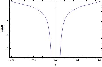
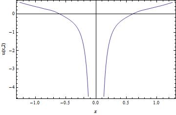
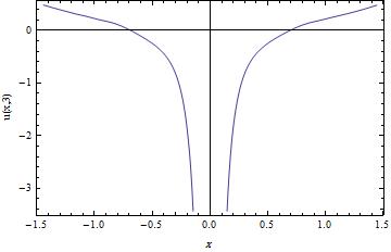
Figure 1. Plot of approximate solution $u(x,t)$ for $t=1,2,3$ and $N=25$ in Problem 1.

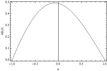
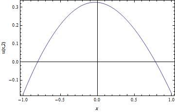
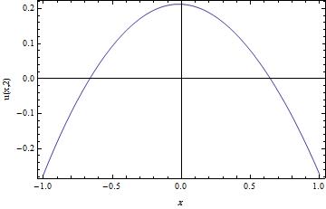
Figure 2. Plot of approximate solution $u(x,t)$ for $t=1,2,3$ and $N=25$ in Problem 2.

6.2. Problem 2: CPSM for (5.6)

We can use CPSM for the differential equation (5.6) that obtained the previous section. We consider boundary conditions $f(-1)=f^{\prime}(-1)=f(1)=1$ for this problem. After inserting the formulas (6.8), we have the reduce form:

$$\left\{\begin{array}[]{l}{\displaystyle{4tf^{2}(\zeta_{i})\left(\sum_{j=0}^{N}d_{ij}^{(3)}f(\zeta_{j})\right)-12tf(\zeta_{i})\left(\sum_{j=0}^{N}d_{ij}f(\zeta_{j})\right)\left(\sum_{j=0}^{N}d_{ij}^{(2)}f(\zeta_{j})\right)+8t\left(\sum_{j=0}^{N}d_{ij}f(\zeta_{j})\right)^{3}}}\\ {\displaystyle{+24tf^{2}(\zeta_{i})\ln\left(\frac{f(\zeta_{i})}{\sqrt[4]{t}}\right)\left(\sum_{j=0}^{N}d_{ij}f(\zeta_{j})\right)-2f^{3}(\zeta_{i})\ln\left(\frac{f(\zeta_{i})}{\sqrt[4]{t}}\right)-f^{3}(\zeta_{i})=0,}\qquad i=0,\cdots,N-2.}\\[14.22636pt] {\displaystyle{f(\zeta_{N})=f(\zeta_{0})=1,\quad\sum_{j=0}^{N}d_{Nj}f(\zeta_{j})=1.}}\end{array}\right.$$

Similar to the Problem 1, for any $t$, we get a system of $N-1$ nonlinear equations and $N-1$ unknown parameters $f(\zeta_{i})$ for $i=1,\cdots,N-1$ . Accuracy of the approximate solutions for $N=25$ and $t=1,2,3$ is observable in Table 2. Also, by (5.5) we can show the behaviors of $u(x,t)$ for $N=25$ and $t=1,2,3$ in Figures 2.

7. Conclusion and Results

Lie point symmetries of the Korteweg-de Vries equation with power-law nonlinearity (1.1) in a particular form of is $a(t)=6,n=1,b(t)=1$ with $c(t)=0$ and $l(t)=-1/2t$, form a three dimensional Lie symmetry algebra. The invariant solution of these symmetries is reduced The optimal system of one-dimensional Lie subalgebras associated to this symmetry algebra is generated by two vector fields.

The Chebyshev pseudo-spectral method (CPSM) as a numerical analysis is applied for invariant solutions. In this method, we use the Chebyshev-Gauss-Lobatto points as collocation points.

References

• [1] A. Biswas, Solitary wave solution for KdV equation with power-law nonlinearity and time-dependent coefficients, Nonlinear Dyn (2009) 58: 345-348.
• [2] A. G. Johnpillai, C. M. Khalique and A. Biswas,Exact solutions of the mKdV equation with time-dependent coeffcients, Math. Commun. 16(2011), 509–518.
• [3] S. Lie, Arch. for Math. 6 (1881) 328–368; translation by N.H. Ibragimov: S. Lie, On integration of a class of linear partial differential equations by means of definite integrals, in: N.H. Ibragimov (Ed.), CRC Handbook of Lie Group Analysis of Differential Equations in 3 Volumes, vol. 2, 1994, pp. 473–508.
• [4] F. Gungor, V. I. Lahno, R. Z. Zhdanov, Symmetry classification of KdV-type nonlinear evolution equations, J. Math. Phys., Vol. 45, No. 6, 2004.
• [5] M. Nadjafikhah, R. Bakhshandeh Chamazkoti, A. Mahdipour-Shirayeh, A symmetry classification for a class of (2+1)-nonlinear wave equation, Nonlinear Analysis 71 (2009) 5164–5169.
• [6] M. Nadjafikhah, R. Bakhshandeh-Chamazkoti, Symmetry group classification for general Burgers’ equation, Commun Nonlinear Sci Numer Simulat 15 (2010) 2303–2310.
• [7] M. Nadjafikhah, R. Bakhshandeh-Chamazkoti, Preliminarily group classification of a class of 2D nonlinear heat equations, IL NUOVO CIMENTO, Vol. 125 B, N. 12, 1465–1478.
• [8] P.J. Olver, Equivalence, Invariants, and Symmetry, Cambridge University Press, (1995).
• [9] L. V. Ovsiannikov, Group analysis of differential equations, New York: Academic Press; 1982.
• [10] R. Peyret, Spectral methods for incompressible viscous flow, Applied Mathematical Sciences 148, Springer-Verlag, 2002.
• [11] S. Zhang, Exact solution of a KdV equation with variable coefficients via exp-function method, Nonlinear Dyn. 52(1-2), 11-17 (2007).