3D MHD simulation of linearly polarised Alfven wave dynamics in Arnold-Beltrami-Childress magnetic field

Abstract

Previous studies (e.g. Malara et al ApJ, 533, 523 (2000)) considered small-amplitude Alfven wave (AW) packets in Arnold-Beltrami-Childress (ABC) magnetic field using WKB approximation. They draw a distinction between 2D AW dissipation via phase mixing and 3D AW dissipation via exponentially divergent magnetic field lines. In the former case AW dissipation time scales as $S^{1/3}$ and in the latter as $\log(S)$, where $S$ is the Lundquist number. In this work linearly polarised Alfven wave dynamics in ABC magnetic field via direct 3D MHD numerical simulation is studied for the first time. A Gaussian AW pulse with length-scale much shorter than ABC domain length and a harmonic AW with wavelength equal to ABC domain length are studied for four different resistivities. While it is found that AWs dissipate quickly in the ABC field, contrary to an expectation, it is found the AW perturbation energy increases in time. In the case of the harmonic AW the perturbation energy growth is transient in time, attaining peaks in both velocity and magnetic perturbation energies within timescales much smaller than the resistive time. In the case of the Gaussian AW pulse the velocity perturbation energy growth is still transient in time, attaining a peak within few resistive times, while magnetic perturbation energy continues to grow. It is also shown that the total magnetic energy decreases in time and this is governed by the resistive evolution of the background ABC magnetic field rather than AW damping. On contrary, when the background magnetic field is uniform, the total magnetic energy decrease is prescribed by AW damping, because there is no resistive evolution of the background. By considering runs with different amplitudes and by analysing the perturbation spectra, possible dynamo action by AW perturbation-induced peristaltic flow and inverse cascade of magnetic energy have been excluded. Therefore, the perturbation energy growth is attributed to a new instability. The growth rate appears to be dependent on the value of the resistivity and the spatial scale of the AW disturbance. Thus, when going beyond WKB approximation, AW damping, described by full MHD equations, does not guarantee decrease of perturbation energy. This has implications for the MHD wave plasma heating in exponentially divergent magnetic fields.

I Introduction

Damping of magnetohydrodynamic (MHD) waves is of importance to the solar coronal heating problem (e.g. Ref.Aschwanden (2005) and references therein) and Tokamak plasmas Hung and Hassam (2013); Podestà et al. (2013); Farmer and Morales (2013). Phase mixing of harmonic Alfven waves (AW), which propagate in plasma which has a density inhomogeneity in transverse to the uniform background magnetic field (UBMF) direction, results in their fast damping in the density gradient regions. In this case the dissipation time scales as $\tau_{D}\propto S^{1/3}$. Where $S=LV/\eta\propto 1/\eta$ is the Lundquist number. $\eta=1/(\mu_{0}\sigma)$ is plasma resistivity, while $L$ and $V$ are characteristic length- and velocity- scales of the system. This is a consequence of the fact that AW amplitude damps in time as $B_{y}(x,z,t)\propto\exp(-\eta C^{\prime}_{A}(x)^{2}t^{3}k^{2}/6)$, where symbols have their usual meaning and $C^{\prime}_{A}(x)$ denotes Alfven speed derivative in the density inhomogeneity direction Heyvaerts and Priest (1983). Phase mixing of Alfven waves which have Gaussian profile along the background magnetic field results in somewhat slower, power-law damping, $B_{y}\propto t^{-3/2}$, as established in Ref.Hood et al. (2002), whilst more elegantly (in mathematical sense) derived in Ref. Tsiklauri et al. (2003). In a different physical contexts it was shown that exponentially diverging magnetic field lines provide even faster damping $B_{y}=\exp\left(-A_{1}\exp(A_{2}t)\right)$ Similon and Sudan (1989); De Moortel et al. (2000); Smith et al. (2007), resulting in the wave damping timescale as $\tau_{D}\propto\log(S)$.

Ref.Malara et al. (2000) considered small-amplitude AW packets in WKB approximation in Arnold-Beltrami-Childress (ABC) magnetic field, which for certain set of parameters and in known regions of space possesses property of exponentially diverging magnetic fields. Using WKB reduced version of MHD equations they have convincingly demonstrated that when a random number of AW packets are injected in the said ABC field, two distinct populations emerge: (i) ones that dissipate quickly whose damping time $\tau_{D}\propto\log(S)$ and (ii) slowly dissipating AW packets whose damping time scales as $\tau_{D}\propto S^{1/3}$. Moreover, they have established that quickly dissipating AW packets can be associated with damping in exponentially divergent magnetic field regions of the simulation domain, while slowly dissipating AW packets damp in smooth, magnetic-flux-tube-like regions of space. Also, exponentially diverging magnetic fields were discussed in the context of magnetic reconnection Boozer (2012a, b).

To our knowledge the present study is the first that investigates AW damping in ABC magnetic fields using a general, rather than WKB version of 3D resistive MHD equations. Therefore the present work can account for (i) time evolution of the background magnetic field and (ii) the effect of launched Alfvenic waves on the physical system. The latter is not at all a trivial matter, as there are works Grappin et al. (2008) that show in the solar coronal plasma context that directly coupling the low beta coronal evolution to prescribed photospheric motions of the magnetic footpoints allows strong magnetic energy accumulation in the corona. They argue that this amounts to ignoring a possible feedback from coronal loops on photospheric motions. However, the energy injected into the corona comes from the photosphere, so in principle the coronal loop might act as a conduit communicating photospheric dynamics from one region to another.

Section II presents the model and results. Section III summarises the main findings.

II The model and results

The numerical simulations presented here are performed using Lare3d Arber et al. (2001) – a Lagrangian remap code for solving non-linear MHD equations in 3D spatial dimensions. The code is second order accurate in space and time. The use of shock viscosity and gradient limiters make the code ideally suited to shock calculations. The code is available for download from http://ccpforge.cse.rl.ac.uk/gf/project/lare3d/.

The considered numerical runs with their identifying names used throughout this paper are shown in Table 1.

Table 1: Numerical simulation summary table: Columns from left to right indicate: (i) numerical simulation run identification, (ii) type of background magnetic field used, (iii) AW perturbation type (”pulse” stands for ”Gaussian pulse” and ”harm.” stands for ”harmonic”), (iv) resistivity $\hat{\eta}$ (in units of $\mu_{0}L_{0}C_{A}$), (v) end simulation time (in units of $\tau_{A}$), (vi) pertaining movie numbers, (vii) pertaining figure numbers.

$$\begin{array}[]{lllllll}\hline\cr\vskip 3.0pt plus 1.0pt minus 1.0pt\cr\mathrm{Run}&\mathrm{Backgr.}&\mathrm{Perturb.}&\mathrm{Resis-}&t_{end}&\mathrm{Movies}&\mathrm{Figs.}\\ \mathrm{ID}&\mathrm{field}&\mathrm{type}&\mathrm{tivity}&[\tau_{A}]&\mathrm{}&\mathrm{}\\ \vskip 3.0pt plus 1.0pt minus 1.0pt\cr\hline\cr\mathrm{con_{e}}&\mathrm{const}||z&\mathrm{none}&5\times 10^{-4}&20&1,2&1,2\\ \mathrm{con_{p}}&\mathrm{const}||z&\mathrm{pulse}&5\times 10^{-4}&20&1&1\\ \mathrm{con_{h}}&\mathrm{const}||z&\mathrm{harm.}&5\times 10^{-4}&20&2&2\\ \mathrm{abc_{e}0}&\mathrm{ABC}&\mathrm{none}&0&20&1&3\\ \mathrm{abc_{e}1}&\mathrm{ABC}&\mathrm{none}&5\times 10^{-4}&10\pi&3,4,5&3,4,6,7,9,10\\ \mathrm{abc_{e}2}&\mathrm{ABC}&\mathrm{none}&1\times 10^{-4}&10\pi&\mathrm{none}&6,7\\ \mathrm{abc_{e}3}&\mathrm{ABC}&\mathrm{none}&5\times 10^{-5}&10\pi&\mathrm{none}&6,7\\ \mathrm{abc_{e}4}&\mathrm{ABC}&\mathrm{none}&1\times 10^{-5}&10\pi&\mathrm{none}&6,7\\ \mathrm{abc_{p}1}&\mathrm{ABC}&\mathrm{pulse}&5\times 10^{-4}&10\pi&4&6,8,9\\ \mathrm{abc_{p}2}&\mathrm{ABC}&\mathrm{pulse}&1\times 10^{-4}&10\pi&\mathrm{none}&6\\ \mathrm{abc_{p}3}&\mathrm{ABC}&\mathrm{pulse}&5\times 10^{-5}&10\pi&\mathrm{none}&6\\ \mathrm{abc_{p}4}&\mathrm{ABC}&\mathrm{pulse}&1\times 10^{-5}&10\pi&\mathrm{none}&6\\ \mathrm{abc_{h}1}&\mathrm{ABC}&\mathrm{harm.}&5\times 10^{-4}&10\pi&5&7,10\\ \mathrm{abc_{h}2}&\mathrm{ABC}&\mathrm{harm.}&1\times 10^{-4}&10\pi&\mathrm{none}&7\\ \mathrm{abc_{h}3}&\mathrm{ABC}&\mathrm{harm.}&5\times 10^{-5}&10\pi&\mathrm{none}&7\\ \mathrm{abc_{h}4}&\mathrm{ABC}&\mathrm{harm.}&1\times 10^{-5}&10\pi&\mathrm{none}&7\\ \mathrm{abc_{a}1}&\mathrm{ABC}&\mathrm{pulse}&5\times 10^{-4}&10\pi&\mathrm{none}&8\\ \mathrm{abc_{a}2}&\mathrm{ABC}&\mathrm{pulse}&5\times 10^{-4}&10\pi&\mathrm{none}&8\\ \vskip 3.0pt plus 1.0pt minus 1.0pt\cr\hline\cr\end{array}$$

Figure 1: Time evolution of an amplitude, normalised to its initial value, for the case of Alfven pulse in uniform magnetic field. The thin solid line corresponds to the asymptotic solution for large times, Eq.(1). A more general analytical form Eq.(2) is plotted with stars connected by thick line. Crosses and open diamonds are numerical simulation results in the strongest density gradient point $x=(155/512)\times(2\pi)=1.90214$ and away from the gradient $x=(1/512)\times(2\pi)=0.0122718$ (first grid cell in $x$-direction), respectively.

Figure 2: As in Fig.(1) but for the case of harmonic AW, except for there is no thin solid line and an analytical solution is according to Eq.(3) (stars connected by thick line). The crosses (simulation data) practically overlap with the analytical solution.

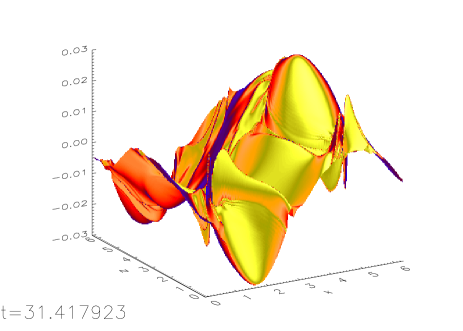
Figure 3: $B_{y}(x,y=y_{max}/2,z,t_{end})-B_{y0}(x,y=y_{max}/2,z,t_{end})$ shaded surface plot, i.e. difference between the magnetic field y-component in the case of ABC field without AW pulse but with resistivity $\hat{\eta}=5\times 10^{-4}$, i.e. numerical run $\mathrm{abc_{e}1}$, (denoted by $B_{y}(x,y=y_{max}/2,z)$ in the animated version of this figure i.e. Movie 3 from Ref.mov ) and magnetic field y-component in the case of ABC field without AW pulse and without resistivity $\hat{\eta}=0$, i.e. numerical run $\mathrm{abc_{e}0}$, (denoted by $B_{y0}(x,y=y_{max}/2,z)$ in Movie 3).

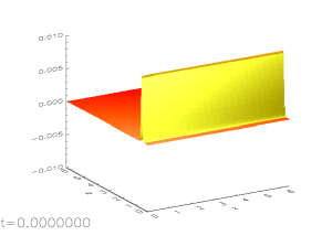
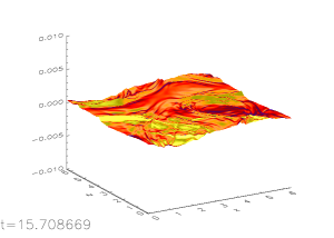
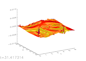
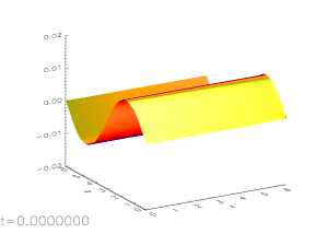
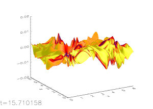
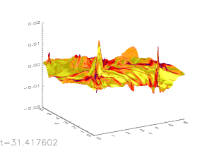
Figure 4: Top panels are three time snapshots $t=0,t=t_{end}/2,t=t_{end}$ of $B_{y}(x,y=y_{max}/2,z)-B_{y0}(x,y=y_{max}/2,z,t)$ shaded surface plot, i.e. difference between the magnetic field y-component in the case of ABC field with AW Gaussian pulse and with resistivity $\hat{\eta}=5\times 10^{-4}$, i.e. numerical run $\mathrm{abc_{p}1}$, (denoted by $B_{y}(x,y=y_{max}/2,z)$ in the the animated version of this figure i.e. Movie 4 from Ref.mov ) and magnetic field y-component in the case of ABC field without a AW pulse and with the same resistivity $\hat{\eta}=5\times 10^{-4}$, i.e. numerical run $\mathrm{abc_{e}1}$, (denoted by $B_{y0}(x,y=y_{max}/2,z)$ in Movie 4). Bottom panels are the same as top ones, but for the case of harmonic wave (the animated version of this figure’s bottom row is shown in Movie 5 from Ref.mov ), therefore now corresponding numerical runs used in the subtraction are $\mathrm{abc_{h}1}$ and $\mathrm{abc_{e}1}$.

Figure 5: Energies for the case of UBMF integrated over entire simulation box. In particular, the panels show: (a) full magnetic energy (background plus AW perturbation), $E_{mag}$, (b) full kinetic energy (background plus AW perturbation), $E_{kin}$, (c) internal energy, $E_{int}$, (d) magnetic perturbation energy, according to Eq.(5), $E_{mag}^{\prime}$, (e) resistive energy (Ohmic heating), $E_{res}$, (f) total energy, $E_{tot}\equiv E_{mag}+E_{kin}+E_{int}$. In all panels solid line is for run $\mathrm{con_{p}}$, while dotted line is for $\mathrm{con_{h}}$.

Figure 6: Similar to Fig. 5 but here solid, dotted, dashed, dash-dotted lines pertain to the runs $\mathrm{abc_{p}1}$, $\mathrm{abc_{p}2}$, $\mathrm{abc_{p}3}$ and $\mathrm{abc_{p}4}$ respectively and panel (e) here is replaced by kinetic perturbation energy, $E_{kin}^{\prime}$, according to Eq.(6).

Figure 7: Similar to Fig. 5 but here solid, dotted, dashed, dash-dotted lines pertain to the runs $\mathrm{abc_{h}1}$, $\mathrm{abc_{h}2}$, $\mathrm{abc_{h}3}$ and $\mathrm{abc_{h}4}$ respectively and panel (e) here is replaced by kinetic perturbation energy, $E_{kin}^{\prime}$, according to Eq.(6).

Although Lare3d has been extensively tested before, there were several significant recent updates. Thus, we start from presenting numerical code validation. This is done showing the results from two numerical runs of the code. In all our numerical simulations we use a 3D box with 512³ uniform grids in $x$,$y$, and $z$ direction having length of $2\pi$ in each spatial direction. Distance, magnetic field and density are normalised to their background values $L_{0},B_{0},\rho_{0}$. Whereas, velocity and time to the respective Alfven values $C_{A}=B_{0}/\sqrt{\mu_{0}\rho_{0}}$ and $\tau_{A}=L_{0}/C_{A}$. Boundary conditions are periodic in all three spatial directions. When using resistivity we have tested cases with zero and non-zero values of the resistivity in the ghost cells around the physical simulation domain. No noticeable difference was found by setting resistivity to zero in the ghost cells. For the first two runs, normalised, uniform magnetic field, of strength unity, is in $z$-direction. Plasma density has a profile in $x$-direction $\rho(x)=1+9\exp(-(x-\pi)^{4})$. For the runs with ABC magnetic field (see below) the density is set constant $\rho=1$. Plasma beta and gravity are set to zero in all numerical runs. We launch: (i) a Gaussian pulse which has two components, $B_{y}=0.01\exp(-(z-0.5)^{2}/(2\times 0.05^{2}))$, $V_{y}=-0.01\exp(-(z-0.5)^{2}/(2\times 0.05^{2}))/\sqrt{\rho(x)}$, making it a linearly polarised AW packet, which has an amplitude of $0.01$ (except for numerical runs $\mathrm{abc_{a}1}$ where amplitude is $0.05$ and $\mathrm{abc_{a}2}$ where amplitude is $0.1$), starts at $z=0.5$ and has a width of $0.05$. (ii) a harmonic wave which has two components, $B_{y}=0.01\sin(z)$, $V_{y}=-0.01\sin(z)/\sqrt{\rho(x)}$, making it also a linearly polarised AW packet, with an amplitude of $0.01$, and spanning the full domain length in $z$ direction (contrary to pulse case that is rather spatially localised). Plasma viscosity is set to zero, while first and second shock viscosity coefficients are 0.01 and 0.05 (see Ref.Arber et al. (2001) for further details). Figs. 1 and 2 show time evolution of the AW damping for plasma resistivity of $\hat{\eta}=5\times 10^{-4}$ for the cases of Gaussian pulse and harmonic wave respectively (runs $\mathrm{con_{p}}$ and $\mathrm{con_{e}}$ from Table 1). The resistivity is in units of $\mu_{0}L_{0}C_{A}$. Thus, $1/{\hat{\eta}}=S$ is the Lundquist number. In the both figures, crosses and open diamonds are numerical simulation results in the strongest density gradient point $x=(155/512)\times(2\pi)=1.90214$ and away from the gradient $x=(1/512)\times(2\pi)=0.0122718$ (first grid cell in $x$-direction). We essentially plot the simulation values by tracing crests of the numerical arrays $B_{y}(155,256,z)$ and $B_{y}(1,256,z)$ that track damping of the AW. In Fig. 1 the thin solid line corresponds to the asymptotic solution for large times

$$B_{y}=t^{-3/2}/(5\sqrt{2\pi C^{\prime}_{A}(x)^{2}/3}),$$ (1)

i.e. true for $t\gg\tau_{A}$, while a more general analytical form Hood et al. (2002); Tsiklauri et al. (2003)

$$B_{y}={\frac{\alpha_{0}}{\sqrt{1+\eta C^{\prime}_{A}(x)^{2}t^{3}/3\sigma^{2}}}}\\ \exp{\left[{-{\frac{(z-C_{A}(x)t)^{2}}{2(\sigma^{2}+\eta C^{\prime}_{A}(x)^{2}t^{3}/3)}}}\right]},$$ (2)

is plotted with stars connected by thick line. In Fig. 2 stars connected by thick line correspond to the analytical solution Heyvaerts and Priest (1983)

$$B_{y}=\exp(-\eta C^{\prime}_{A}(x)^{2}t^{3}k^{2}/6)\exp(-ik(z-C_{A}(x)t)).$$ (3)

Note in Fig. 2 that away from the density gradient AW is not damped noticeably (open diamonds near top of the figure). We see that AW damping closely follows the analytical theory expressions. The percentage errors at $t=20$ Alfven times are 2.6% for the case of Gaussian pulse and 1.1% in the case of harmonic wave. Naturally, the pulse is more spatially localised while the harmonic wave spans entire domain length in $z$ direction, thus when resolved by 512 grid points the larger error is for the case of the Gaussian pulse. Movies 1 and 2 from Ref.mov show time evolution of AW damping in the Gaussian pulse and harmonic wave respectively. Note how AWs quickly damp (contours thin or fade away) in the density inhomogeneity regions $x\approx 1.5-2$ and $x\approx 4.0-4.5$ where the wave fronts bend strongly starting at $t=0$ from initially flat profiles. It is this derivative of the Alfven speed, $C^{\prime}_{A}(x)$, in $x$-direction, which enters equations (1)–(3), that is responsible for the fast damping of the AW. Away from the density gradient regions much slower damping, $\exp(-\eta k^{2}t)\propto\exp(-t)$, operates, which is barely noticeable on the time-scales concerned.

It should be noted we have checked how well the resistive equilibrium holds in the case of UBMF. This was done in runs $\mathrm{con_{e}}$ from Table 1. We confirm that e.g. the difference of magnetic field component $B_{y}(x,y=y_{max}/2,z,t=t_{end}=20)$ with its initial value $B_{y}(x,y=y_{max}/2,z,0)$ with $\hat{\eta}=5\times 10^{-4}$ does not exceed $3\times 10^{-14}$, i.e. resistive equilibrium holds and subtracting the modification of $B_{y}(x,y=y_{max}/2,z,t)$ from the ideal (non-resistive) plasma case does not make any difference. However, the same does not hold for the ABC field and the resistive evolution of the background magnetic field turns out to be significant.

Figure 8: Magnetic perturbation energy, normalised to its initial value, according to Eq.(5), $E_{mag}^{\prime}/E_{mag}^{\prime}(0)$, for runs $\mathrm{abc_{p}1}$ (with the pulse amplitude $0.01$) solid line, $\mathrm{abc_{a}1}$ (with pulse amplitude $0.05$) dotted line and $\mathrm{abc_{a}2}$ (with pulse amplitude $0.1$) dashed line.

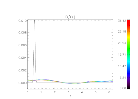
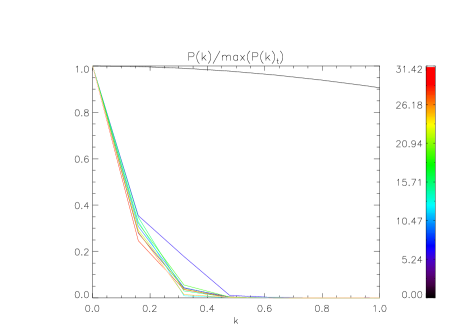
Figure 9: Top panel: time evolution of physical quantity $B_{y}^{*}(z)$ calculated by Eq.(7) for the case of Gaussian AW pulse. The numerical runs used in the subtraction are $\mathrm{abc_{p}1}$ and $\mathrm{abc_{e}1}$. Bottom panel: time evolution of the Fourier spectrum of $B_{y}^{*}(z)$ from the top panel. See text for the normalisation of the Fourier spectrum used. Colour bar and colour lines show the advance of simulation time from $t=0$ (black) to $10\pi$ (red).

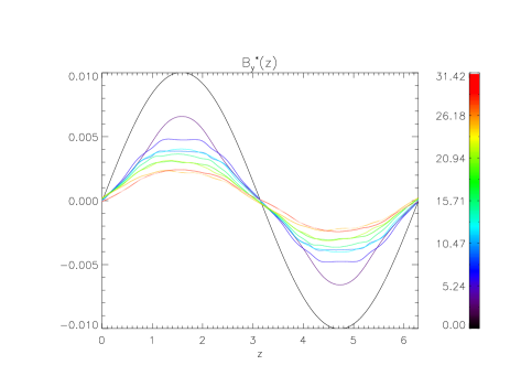
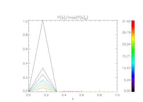
Figure 10: The same as in Fig. 9 but for the case of the harmonic AW. The numerical runs used in the subtraction here are $\mathrm{abc_{h}1}$ and $\mathrm{abc_{e}1}$.

The ABC magnetic field is given by the following expressions Malara et al. (2000):

$$B_{x}(x,y,z)=A\sin(z)+C\cos(y),$$

$$B_{y}(x,y,z)=B\sin(x)+A\cos(z),$$

$$B_{z}(x,y,z)=C\sin(y)+B\cos(x).$$

Following Ref.Malara et al. (2000) we fix the values of the coefficients as $A=\sqrt{1/3},\,B=1,\,C=\sqrt{2/3}$. This choice insures that ABC field has essentially entangled magnetic flux tube-like structure along $z$-coordinate, with regions of space that have regular (nearly uniform) magnetic flux-tubes and also regions that have exponentially divergent magnetic fields (cf. Fig. 1 from Ref.Malara et al. (2000)). It is easy to show by an analytical calculation that in the ideal ($\hat{\eta}=0$) case for the ABC field the usual plasma MHD equilibrium equation $\nabla(p+\vec{B}^{2}/(2\mu_{0}))=(\vec{B}\cdot\nabla)\vec{B})/\mu_{0}$ holds when pressure $p$ is constant (or zero). However, the latter equation ignores the resistive effects and when included these drive the magnetic field out of equilibrium. The deviation from the initial equilibrium is studied in Fig. 3 and its animated version Movie 3 from Ref.mov , where we plot time dynamics of $B_{y}(x,y=y_{max}/2,z,t)-B_{y0}(x,y=y_{max}/2,z,t)$ shaded surface plot, i.e. difference between the magnetic field y-component in the case of ABC field without AW pulse but with resistivity $\hat{\eta}=5\times 10^{-4}$, i.e. numerical $\mathrm{abc_{e}1}$, (denoted by $B_{y}(x,y=y_{max}/2,z)$ in Movie 3) and magnetic field y-component in the case of ABC field without AW pulse and without resistivity $\hat{\eta}=0$, i.e. numerical $\mathrm{abc_{e}0}$, (denoted by $B_{y0}(x,y=y_{max}/2,z)$ in Movie 3). It can be deduced that the difference attains a value of 0.029228 which is about three times the amplitude of the AW (either Gaussian pulse or harmonic wave). Other ($x$- and $z$-) magnetic field component differences are of the same order. It should be noted that the difference scales with $\hat{\eta}$, i.e. in the run $\mathrm{abc_{e}3}$ where $\hat{\eta}=5\times 10^{-5}$ the difference is 0.0029228.

Therefore it is rather important to take into account resistive evolution of the equilibrium of the magnetic field when studying propagation of AWs in ABC fields. In practice this means that when launching AWs we need to correctly single out the magnetic perturbation from the background, i.e. ABC field without an AW pulse but with the same resistivity. This is achieved by calculation using Eq.(5), where $\vec{B}$ (and its components $B_{x}$, $B_{y}$ and $B_{z}$) stands for full magnetic field (background plus AW) while $\vec{B}_{0}$ stands for just background i.e. ABC field without an AW pulse but with the same resistivity.

$$E_{mag}^{\prime}={\frac{1}{2}}\int_{0}^{2\pi}\int_{0}^{2\pi}\int_{0}^{2\pi}[(B_{x}^{2}+B_{y}^{2}+B_{z}^{2})-$$

$$(B_{x0}^{2}+B_{y0}^{2}+B_{z0}^{2})-2\vec{B}_{0}\cdot(\vec{B}-\vec{B}_{0})]dxdydz.$$ (5)

A similar approach is adopted for the velocity perturbations:

$$E_{kin}^{\prime}={\frac{1}{2}}\int_{0}^{2\pi}\int_{0}^{2\pi}\int_{0}^{2\pi}[(V_{x}^{2}+V_{y}^{2}+V_{z}^{2})-$$

$$(V_{x0}^{2}+V_{y0}^{2}+V_{z0}^{2})-2\vec{V}_{0}\cdot(\vec{V}-\vec{V}_{0})]dxdydz.$$ (6)

As with magnetic field in Eq.(6), $\vec{V}$ (and its components $V_{x}$, $V_{y}$ and $V_{z}$) stands for full velocity field (background plus AW) while $\vec{V}_{0}$ stands for just background i.e. ABC field without an AW pulse but with the same resistivity.

The dynamics of AW Gaussian pulse and harmonic wave is shown in Fig. 4 with corresponding animated versions presented in Movie 4 and Movie 5 from Ref.mov . It is clear that both AWs damp rather quickly. Note that both in Fig. 1, Fig. 2, and Fig. 4 resistivity is the same ($\hat{\eta}=5\times 10^{-4}$), and the end simulation times are $t_{end}=20$ and $10\pi$, respectively. This shows that in the case of ABC background field the AW damping is faster. Note from the movies that, because of existence of exponentially divergent field line regions, initially flat AW fronts became quickly corrugated via wave refraction, because of rather complicated form of the local Alfven speed $C_{A}(x,y,z)$ prescribed by Eq. (4). As in the case of UBMF, in ABC fields the Gaussian pulse damping is also faster because its strong localisation along $z$-coordinate.

The most interesting findings of this study come to light when investigating the energetics of the AW dynamics/damping. Fig. 5 shows energies for the UBMF. The energies are calculated over entire simulation domain using Lare3d code’s built-in function called $\mathrm{getenergy()}$. The latter takes the averages of $B_{x}^{2}/2$, $B_{y}^{2}/2$ and $B_{z}^{2}/2$ to cell centres and then sums over all simulation cells. The latter function produces magnetic, kinetic, internal and resistive (Ohmic) heating energies. The only exception is panel (d) where magnetic perturbation energy is plotted, according to Eq.(5). Note that in panels (d), in all figures 5, 6, 7 and in Fig. 8, there are only 10 equally spaced data points, while in all other panels there thousands of data points. This is because Lare3d’s $\mathrm{getenergy()}$ outputs energy at every time step, whereas when we use Eqs.(5) and (6), we use IDL’s built in function $\mathrm{int\_tabulated}$, which employs five-point Newton-Cotes integration formula, to do the manual integrations. We have tested energy calculation using $\mathrm{int\_tabulated}$ and $\mathrm{getenergy()}$ and concluded while the both yield similarly close results, $\mathrm{int\_tabulated}$ has a superior accuracy.

One can gather from Fig. 5(a,b,d) that the magnetic, kinetic and AW perturbation magnetic energies start from their respective values and then decrease in time. Whereas internal and resistive heating energies start from zero and increase in time – see Fig. 5(c,e). Note that all of the above energies include contributions from both inhomogeneous density parts where AW damping is rather vigorous and homogeneous density parts where damping is weak. Because density gradient regions are not large, overall AW damping is not strong. Overall, UBMF cases produce the expected result that AW perturbation energy is damped and converted in plasma resistive heating. We see in Fig. 5(f) that the total energy is conserved, indicating that numerical errors (numerical dissipation) are tolerably small.

The most surprising result is obtained in the study of ABC-field energetics, shown in Fig. 6 and Fig. 7. The latter two plots are similar to Fig. 5, but now show energies for the ABC background magnetic field for the Gaussian pulse and harmonic wave cases, respectively. The four curves in Fig. 6 and Fig. 7 correspond to the four different resistivities, as detailed in Table 1.

One can gather from Fig. 6(a) and Fig. 7(a) that the total magnetic energies start from their respective initial values and then decrease in time. Note that, naturally, larger resistivity results in larger dissipation of magnetic energy. The total kinetic energy seems to transiently increase, see solid curves in Fig. 6(b) and Fig. 7(b), and this can be attributed to the resistive evolution of the background. The transient increase in the total kinetic energy can be only seen for $\hat{\eta}=5\times 10^{-4}$. It is not certain, but is a likely possibly that for smaller resistivity (dotted, dashed and dash-dotted curves in Fig. 6(b) and Fig. 7(b)) will behave in a similar time-transient way.

Note that Figs. 6(a), (b) and (c) are nearly identical to Figs. 7(a), (b) and (c), with the exception of Fig. 7(b), where a small ”wiggle” in the lower left corner is noticeable. This similarity can be attributed to the fact that the behavior of the energies is prescribed by the resistive evolution of the ABC background magnetic field rather than AW perturbation damping. The proof of this can be found by looking at Figs. 5(a), (b) and (c) where cases with UBMF are shown. Here the corresponding energies behave distinctly differently in the case of different types of AW perturbations, because now their time evolution is prescribed by AW damping and there is no resistive evolution of the uniform background magnetic field.

Because in panels Fig. 6(d) and Fig. 7(d) behaviour of $E_{mag}^{\prime}$ becomes different (at least on the timescales considered), let us estimate the resistive times for the Gaussian and harmonic AWs. Based on the one dimensional diffusion equation, $\partial B/\partial t={\hat{\eta}}\partial^{2}B/\partial^{2}_{xx}$, which governs phase-mixed AW damping, we define the resistive time as $\tau_{r}=L^{2}/{\hat{\eta}}$, where reciprocal of $1/L\approx\partial/\partial x$ is the length-scale of variation of magnetic field in AW. Therefore, for the largest value of resistivity considered, $\hat{\eta}=5\times 10^{-4}$, we have $\tau_{r}=(2\pi)^{2}/5\times 10^{-4}=7.9\times 10^{4}\tau_{A}$ for the harmonic AW. For Gaussian pulse case for the same resistivity $\tau_{r}=(0.05)^{2}/5\times 10^{-4}=5\tau_{A}$. Here, Gaussian pulse width is taken as 0.05 which can be also inferred from the black solid curve in the top panel of Fig.9. We gather from Fig. 6(d) and Fig. 6(e) that in the case of the Gaussian AW pulse the velocity perturbation energy growth is transient in time for $\hat{\eta}=5\times 10^{-4}$, attaining a peak within few resistive times $\tau_{r}=5$, while magnetic perturbation energy continues to grow. The numerical values that can be also read from Fig. 6(d) and Fig. 8 are such that $E_{mag}^{\prime}(t=t_{end})/E_{mag}^{\prime}(0)=49.25$ for $\hat{\eta}=10^{-5}$ (dash-dotted curve) and $E_{mag}^{\prime}(t=t_{end})/E_{mag}^{\prime}(0)=16.62$ for $\hat{\eta}=5\times 10^{-4}$ (solid curve). We also gather from Fig. 7(d) and Fig. 7(e) that for $\hat{\eta}=5\times 10^{-4}$, in the case of the harmonic AW, the perturbation energy growth is transient in time, attaining peaks in both velocity ($t\approx 25$) and magnetic ($t\approx 5$) perturbation energies within timescales much smaller than the resistive time $\tau_{r}=7.9\times 10^{4}$. The numerical values that can be also read from Fig. 7(d) are such that $max(E_{mag}^{\prime}(t)/E_{mag}^{\prime}(0))=1.49$ for $\hat{\eta}=10^{-5}$ (dash-dotted curve) and $max(E_{mag}^{\prime}(t)/E_{mag}^{\prime}(0))=1.35$ for $\hat{\eta}=5\times 10^{-4}$ (solid curve). Figures with the internal (Fig. 6(c) and 7(c)) and resistive heating energies (not shown here) start from zero and increase in time. Again larger resistivity results in the larger growth. The unexpected result is that the magnetic perturbation energy, $E_{mag}^{\prime}$, calculated using Eq.(5), increases in time, in the case of Gaussian pulse and time-transiently in the case of harmonic AW, despite that (i) AW damps (cf. Fig. 4) and (ii) total magnetic energy decreases in time (cf. Fig. 6(a) and 7(a)).

The initial AW perturbation has $V_{y}$ and $B_{y}$ components and whilst the amplitudes are small, 0.01, one could conjecture that even a small non-linearity can produce a flow by a peristaltic mechanism Aarts and Ooms (1998). As the AWs travel along the field lines (due to the plasma frozen-in condition that is somewhat offset by a finite resistivity) the flow that derives from the AW perturbation might generate the magnetic field by the dynamo action. It is a well-known fact that flows that have similar mathematical structure to Eq.(4) result in a magnetic dynamo action. We explore this in Fig. 8 where essentially we repeat numerical run $\mathrm{abc_{p}1}$, which has pulse amplitude of $0.01$, for two additional pulse amplitudes $0.05$ and $0.1$. Because the strength of the peristaltic flow is an effect that is proportional to the amplitude squared (i.e. quadratical non-linearity effect), one would expect a stronger growth of AW magnetic perturbation energy with an increase of amplitude. We gather from Fig. 8 that the increase of amplitude does not alter AW magnetic perturbation energy growth. Thus both peristalsis and magnetic dynamo action can be excluded as a cause of AW magnetic perturbation energy growth.

Next, we conjecture that magnetic perturbation energy growth can be attributed to the inverse cascade of magnetic energy Kraichnan (1967). The conjecture of the inverse cascade has strong support from both computer simulations Sommeria (1986) and laboratory experiments Bardóczi et al. (2012). We explore this idea in Fig. 9 for the case of the Gaussian AW pulse and in Fig. 10 for the case of the harmonic AW. Colour bar and colour lines in both figures show advance of simulation time from $t=0$ (black) to $10\pi$ (red). Top panels in both figures show time evolution of physical quantity $B_{y}^{*}(z)$ calculated by

$$B_{y}^{*}(z)={\frac{1}{4\pi^{2}}}\int_{0}^{2\pi}\int_{0}^{2\pi}(B_{y}-B_{y0})dxdy,$$ (7)

where $B_{y}$ stands for full magnetic field (background plus AW) while $B_{y0}$ stands for just background i.e. ABC field without an AW pulse but with the same resistivity. We clearly see at $t=0$ a Gaussian pulse with width 0.05 (Fig. 9) and harmonic wave with wavelength of $2\pi$ (Fig. 10). Time evolution can be tracked by looking at different colour lines which represent time interval of $\pi$ (ten of such intervals altogether). We see in Fig. 9 that the Gaussian pulse quickly diffuses away by increasing its width. In Fig. 10 we see that despite such complicated behaviour as seen in Fig. 4, after all the wave refraction, due to coordinate dependent Alfven speed is integrated out, the sinusoidal shape is still retained and we only see the AW amplitude fading away. Note that the wave is not standing but moving many times in the periodic box – it is the choice of snapshot times create this stroboscopic effect. Bottom panel of Fig. 9 shows time evolution of the Fourier spectrum. Each different colour line is normalised to a maximum value at different times (hence subscript in $max(P(k)_{t})$) therefore all curves start from unity. Black curve that can be seen in the upper part of the plot is actually a Gaussian, because Fourier transform of a Gaussian is a Gaussian. It appears as a very flat Gaussian because we wanted to show clearly later time evolution, thus we had to restrict the range of wavenumbers $k$ to unity. We see no evidence for the inverse cascade because no more wave power is seen at smaller $k$ for large times. We see a simple diffusion process of AW, when initially narrow Gaussian pulse widens by diffusion (via resistivity). Bottom panel of Fig. 10 also shows time evolution of the Fourier spectrum but for harmonic AW. Now each different colour line is normalised to a maximum value at $t=0$ (hence subscript in $max(P(k)_{0})$) therefore black curve peaks with the value of unity. At all later times the peak amplitudes decrease because wave damps. The prominent peak is at $1/(2\pi)=0.159$, as expected of Fourier transform of $\sin(z)$. More importantly, as the time progresses the peak does not shift in $k$, therefore again we see no evidence for the inverse cascade.

III conclusions

Motivated by Ref.Malara et al. (2000), who studied small-amplitude AW packets in WKB approximation in ABC magnetic fields, we relax the approximation and solve fully 3D MHD problem. Ref.Malara et al. (2000) drew a distinction between 2D AW dissipation via phase mixing, with AW dissipation time scaling of $S^{1/3}$, and 3D AW dissipation via exponentially divergent magnetic field lines, with dissipation time scaling of $\log(S)$. They also suggested that for $S\leq 4\times 10^{6}$ no clear distinction could be drawn between the two regimes, as the large resistivity $\hat{\eta}=1/S=2.5\times 10^{-7}$ made damping too strong. In the current study because we used full 3D MHD simulations (as opposed to WKB approximation used by Ref.Malara et al. (2000)) we could not access large enough end simulation times for the damping to be noticeable in the small resistivity regime. Thus testing of the above AW damping scaling laws within full MHD is still not achieved. However, we found other interesting effects: We studied two types of AW perturbations: (i) a Gaussian pulse with length-scale much shorter than ABC domain length and (ii) a harmonic AW with wavelength equal to ABC domain length. We have shown that AWs dissipate quickly in the ABC field. Our results are surprising in that AWs magnetic perturbation energies increase in time, monotonously or in time-transient manner, depending on the spatial scale of the AW disturbance, within the considered end simulation time. In the case of the harmonic AW the perturbation energy growth is transient in time, attaining peaks in both velocity and magnetic perturbation energies within timescales much smaller than the resistive time. In the case of the Gaussian AW pulse the velocity perturbation energy growth is also transient in time, attaining a peak within few resistive times, while magnetic perturbation energy continues to grow. We find that the total magnetic energy decreases in time and this is prescribed by the resistive evolution of the background ABC magnetic field rather than AW damping. Moreover, in the case of uniform background magnetic field, the total magnetic energy decrease in time is prescribed by AW damping, because of the absence of resistive evolution of the background. We then considered runs with different amplitudes and performed analysis of the perturbation spectra. We excluded both (i) a possible dynamo action by AW perturbation-induced peristaltic flow and (ii) an inverse cascade of magnetic energy. The only remaining reasonable explanation to the perturbation energy growth is a new instability. The growth rate seems to be dependent of the value of the resistivity and also on the spatial scale of the AW disturbance. Further analysis is needed in order to determine the exact mathematical nature of the growth rate dependence on these parameters.

The main conclusion is that in the complex, exponentially diverging magnetic fields that can occur e.g. in the lower solar corona, in cusps of Earth magnetosphere and/or Tokamak/Stellarator, ABC-like background magnetic field, with periodic boundary conditions, evolve significantly in time caused by the slow diffusion. The deviations from the initial state can be as large as 0.03 (with initial background magnetic fields being of the order of unity) within $10\pi\approx 30$ Alfven times. Thus, the fast damping in these entangled magnetic fields, as predicted by the WKB approximation, seems not to be guaranteed.