Integral Equation Theory for Pair Correlation Functions in a Crystal

Abstract

A method for calculating pair correlation functions in a crystal is developed. The method is based on separating the one- and two- particle correlation functions into the symmetry conserving and the symmetry broken parts. The conserving parts are calculated using the integral equation theory of homogeneous fluids. The symmetry broken part of the direct pair correlation function is calculated from a series written in powers of order parameters and that of the total pair correlation function from the Ornstein- Zernike equation. The results found for a two-dimensional hexagonal lattice show that the method provides accurate and detailed informations about the pair correlation functions in a crystal.

The structural and thermodynamic properties of a classical system can adequately be described in terms of one and two-particle density distributions 1 ; 2 . The one particle density distribution $\rho(\vec{r_{1}})$ gives the probability of finding a particle at position $\vec{r_{1}}$ while the two-particle density distribution $\rho^{(2)}(\vec{r_{1}},\vec{r_{2}})$ gives the probability of finding simultaneously a particle at position $\vec{r}_{1}$ and another particle at position $\vec{r}_{2}$. The pair distribution function $g(\vec{r}_{1},\vec{r}_{2})$ which in the case of a homogeneous system reduces to the radial distribution function (RDF) $g^{(0)}(|\vec{r}_{2}-\vec{r}_{1}|)$ is related to $\rho^{(2)}(\vec{r}_{1},\vec{r}_{2})$ through the relation $\rho^{(2)}(\vec{r}_{1},\vec{r}_{2})=\rho(\vec{r}_{1})\rho(\vec{r}_{2})g(\vec{r}_{1},\vec{r}_{2})$. The two related but different pair correlation functions (PCFs) that appear in the statistical theory of classical systems are the total pair correlation function $h(\vec{r}_{1},\vec{r}_{2})$ defined as $h(\vec{r}_{1},\vec{r}_{2})=g(\vec{r}_{1},\vec{r}_{2})-1$ and the direct pair correlation function (DPCF) $c(\vec{r}_{1},\vec{r}_{2})$. These functions are related through the Ornstein-Zernike (OZ) equation. In a homogeneous system, functions $\rho^{(2)}$, h and c depend only on the inter-particle separation and are function of density $\rho=\frac{N}{V}$ (N being the number of particles in volume V), whereas in an inhomogeneous system they depend on position vectors of particles and are functional of $\rho(\vec{r})$.

A crystal is a system of extreme inhomogeneities where values of $\rho(\vec{r})$ shows several order of magnitude difference between its values on the lattice sites and in the interstitial regions. The periodic structure of crystals allows one to expand $\rho({\roarrow{r}})$ in a Fourier series where the sum is carried over the reciprocal lattice vectors or to write it as a superposition of normalised Gaussians centred around the lattice points. The two-particle density distribution has been approximated as $\rho^{(2)}(\vec{r}_{1},\vec{r}_{2})=\rho(\vec{r}_{1})\rho(\vec{r}_{2})g(|\vec{r}_{2}-\vec{r}_{1}|,\bar{\rho})$ where $g(|\vec{r}_{2}-\vec{r}_{1}|,\bar{\rho})$ is the RDF of a fluid of density $\bar{\rho}$ which is taken to be much lower than the averaged crystal density $\rho$ [3-6]. This amounts to assuming that $g(\vec{r}_{1},\vec{r}_{2})$ is a function of magnitude of the interparticle separation $r=|{\roarrow{r}}_{2}-{\roarrow{r}}_{1}|$ only and also its value is much lower compared to that of a fluid of density $\rho$. Moreover, as the value of $g(r,\bar{\rho})$ decays exponentially, the assumption means that $\rho(\vec{r}_{1})\rho(\vec{r}_{2})h(\vec{r}_{1},\vec{r}_{2})$ is a short range function. On the other hand, calculation of $\rho(\vec{r}_{1})\rho(\vec{r}_{2})h(\vec{r}_{1},\vec{r}_{2})$ done in the harmonic model of crystals shows that this quantity decays as $|\vec{r}_{2}-\vec{r}_{1}|^{-1}$ in three-dimensions 7 ; 8 . Obviously, there is a need to have a theory for PCFs in crystals analogous to the integral equation theory (IET) of homogeneous fluids. Accurate knowledge of PCFs will provide a unified approach to describe both states of matter including the freezing/melting and the solid-solid transitions.

The IET which is used to calculate PCFs in a system interacting via a known pair potential, consists of the OZ equation and a closure relation that relates PCFs to the pair potential 2 . The theory has been used successfully to find values of PCFs h and c in fluids from zero density to close to the freezing density. The application of the theory to crystals or to other inhomogeneous systems has, however, so far been limited 9 . In this context, it is important to note that while the OZ equation is general and applicable to fluids as well as to crystals, the closure relations which have been derived assuming continuous translational symmetry are valid only in homogeneous fluids but not in crystals. This limits the applicability of the existing IET to crystals.

The method proposed here uses the OZ equation and some relations (Eqs (6)-(8)) of density functional theory 2 . The method has following steps: (I) One- and two- particle distribution functions are written as a sum of two contributions; one which preserves the continuous symmetry of the fluid and the other that arises due to breaking of this symmetry at the freezing point. (II) Separation of the OZ equation into two equations; one which contains the symmetry conserving part of $\rho(\vec{r})$, $h(\vec{r}_{1},\vec{r}_{2})$ and $c(\vec{r}_{1},\vec{r}_{2})$ and the other in which the symmetry broken part of these functions appear. (III) Evaluation of symmetry conserving part of correlations and their derivatives with respect to density $\rho$ using the IET of homogeneous systems. (IV) Evaluation of the symmetry broken part of $c(\vec{r}_{1},\vec{r}_{2})$ using a series expressed in powers of order parameters (order parameters are amplitudes of density waves of wavelength $\frac{2\pi}{|G|}$ ; $\vec{G}$ being the reciprocal lattice vectors (RLVs.). (V) Using known values of $c(\vec{r}_{1},\vec{r}_{2})$ the OZ equation is solved to find $h(\vec{r}_{1},\vec{r}_{2})$ for a given $\rho(\vec{r})$. We describe these steps below and report results for a two-dimensional solid of hexagonal symmetry and use Ward identities to check their accuracy.

The OZ equation that connects $h$ and $c$ functions in an inhomogeneous system is,

$$h(\vec{r}_{1},\vec{r}_{2})=c(\vec{r}_{1},\vec{r}_{2})+\int d\vec{r}_{3}c(\vec{r}_{1},\vec{r}_{3})\rho(\vec{r}_{3})h(\vec{r}_{2},\vec{r}_{3}),$$ (1)

The $\rho(\vec{r})$ in a crystal can be written as a sum of two terms $\rho(\vec{r})=\rho+\rho^{b}(\vec{r})$ where $\rho^{b}(\vec{r})=\sum_{G}\rho_{G}\exp(i\vec{G}\cdot\vec{r})$ . Here $\rho$ is the average density of the crystal, $\rho_{G}$ are the order parameters and sum is over the complete set of RLVs. We refer the first term $\rho$ as symmetry conserved and the second $\rho^{(b)}({\roarrow{r}})$ as symmetry broken parts of $\rho(\vec{r})$. Similarly PCFs $h$ and $c$ can be written as a sum of symmetry conserved and symmetry broken parts 10 ;

$$h(\vec{r}_{1},\vec{r}_{2})=h^{(0)}(|\vec{r}_{2}-\vec{r}_{1}|,\rho)+h^{(b)}(\vec{r}_{1},\vec{r}_{2},[\rho])$$

$$c(\vec{r}_{1},\vec{r}_{2})=c^{(0)}(|\vec{r}_{2}-\vec{r}_{1}|,\rho)+c^{(b)}(\vec{r}_{1},\vec{r}_{2},[\rho]).$$ (2)

The symmetry conserved part $(h^{(0)},c^{(0)})$ depends on magnitude of the interparticle separation $r=|\vec{r}_{2}-\vec{r}_{1}|$ and is a function of density $\rho$, whereas the symmetry broken part $(h^{(b)},c^{(b)})$ is functional of $\rho(\vec{r})$ (indicated by square bracket ) and is invariant only under a discrete set of translations corresponding to lattice vectors $\vec{R}_{i}$. The functions $h^{(b)}$ and $c^{(b)}$ can therefore be written as a periodic function of the center of mass variable $r_{c}=\frac{r_{1}+r_{2}}{2}$ and a continuous function of the difference variable $\vec{r}=\vec{r}_{2}-\vec{r}_{1}$ .Thus 8

$$h^{(b)}(\vec{r}_{1},\vec{r}_{2})=\sum_{G}e^{i\vec{G}.\vec{r}_{c}}\>h^{(G)}(\vec{r})$$

$$c^{(b)}(\vec{r}_{1},\vec{r}_{2})=\sum_{G}e^{i\vec{G}.\vec{r}_{c}}\>c^{(G)}(\vec{r}).$$ (3)

Since $h^{(G)}$ and $c^{(G)}$ are real and symmetric with respect to interchange of $\vec{r}_{1}$ and $\vec{r}_{2}$, they satisfy relations $f^{(G)}(\vec{r})=f^{(-G)}(\vec{r})$ and $f^{(G)}(-\vec{r})=f^{(G)}(\vec{r})$ where $f^{(G)}$ is $h^{(G)}$ or $c^{(G)}$.

Substitution of $(2)$ into $(1)$ makes the OZ equation to split into two equations; one that contains $h^{(0)},c^{(0)}$ and $\rho$ whereas the other that contains $h^{(b)},c^{(b)},\rho^{(b)}$ along with $h^{(0)},c^{(0)}$ and $\rho$,

$$h^{(0)}(|\vec{r}_{2}-\vec{r}_{1}|)=c^{(0)}(|\vec{r}_{2}-\vec{r}_{1}|) +\rho\int d\vec{r}_{3}c^{(0)}(|\vec{r}_{3}-\vec{r}_{1}|)$$

$$\times h^{(0)}(|\vec{r}_{3}-\vec{r}_{2}|),$$ (4)

$$h^{(b)}(\vec{r}_{1},\vec{r}_{2})=c^{(b)}(\vec{r}_{1},\vec{r}_{2})+\int d\vec{r}_{3}[\{\rho^{(b)}({\roarrow{r}}_{3})c^{(0)}(|{\roarrow{r}}_{3}-{\roarrow{r}}_{1}|)$$

$$\>+\rho({\roarrow{r}}_{3})c^{(b)}(\vec{r}_{1},\vec{r}_{3})\}h^{(0)}(|\vec{r}_{3}-\vec{r}_{2}|)+\rho({\roarrow{r}}_{3})\{c^{(0)}(|\vec{r}_{3}-\vec{r}_{1}|)$$

$$\>+c^{(b)}(\vec{r}_{1},{{\roarrow{r}}_{3}})\}h^{(b)}(\vec{r}_{2},\vec{r}_{3})].$$ (5)

Eq (4) is the well-known OZ equation of a homogeneous system. It is used along with a closure relation to calculate values of $h^{(0)},c^{(0)}$ and their derivatives with respect to $\rho$ 2 ; 11 ; 12 . Eq (5)is the OZ equation that connects the symmetry broken part of PCFs. We use it to calculate $h^{(b)}(\vec{r}_{1},\vec{r}_{2})$ from known values of $c(\vec{r}_{1},\vec{r}_{2})$ and $\rho(\vec{r})$.

Using the relation 2 ; 13

$$\frac{\delta^{n}c(\vec{r}_{1},\vec{r}_{2})}{\delta\rho(\vec{r}_{3})\cdots\delta\rho(\vec{r}_{n})}=c_{n+2}(\vec{r}_{1},\cdots,\vec{r}_{n}),$$ (6)

where $c_{m}$ is the $m-$ body direct correlation function, and the functional Taylor expansion, one can write the following series for $c^{(b)}(\vec{r}_{1},\vec{r}_{2})$ 10 ,

$$c^{(b)}(\vec{r}_{1},\vec{r}_{2})=\int d\vec{r}_{3}{c_{3}}^{(0)}(\vec{r}_{1},\vec{r}_{2},\vec{r}_{3};\rho)(\rho(\vec{r}_{3})-\rho)$$

$$+\frac{1}{2}\int d\vec{r}_{3}\int d\vec{r}_{4}{c_{4}}^{(0)}(\vec{r}_{1},\vec{r}_{2},\vec{r}_{3},\vec{r}_{4};\rho)(\rho(\vec{r}_{3})-\rho)(\rho(\vec{r}_{4})-\rho)+\cdots,$$ (7)

where $c^{(0)}_{n}$ is the $n-$ body direct correlation function of a homogeneous system of density $\rho$ and $(\rho(\vec{r})-\rho)=\sum_{G}\rho_{G}\exp(i\vec{G}.\vec{r})$. The vales of $c_{m}^{(0)}$ are found from exact relations 13 ,

$$\frac{\partial^{n}c^{(0)}(\vec{r},\rho)}{\partial\rho^{n}}=\int d\vec{r}_{3}\cdots\int d\vec{r}_{n+2}{c^{(0)}}_{n+2}(\vec{r}_{1},\cdots,\vec{r}_{n+2}),$$ (8)

The values of $c^{(0)}(\vec{r},\rho)$ and $\frac{\partial^{n}c^{(0)}(\vec{r},\rho)}{\partial\rho^{n}}$ are calculated from the OZ equation (4) and the Roger-Young closure relation 14 for a system of soft disks interacting via reduced pair potential $\beta u(r)=\frac{\Gamma}{r^{3}}$ where $\beta$ is the inverse temperature in unit of the Boltzmann constant and distance $r$ is measured in unit of $(\frac{1}{\rho})^{\frac{1}{2}}$. The system freezes into a hexagonal crystal at $\Gamma\simeq 10$ 12 ; 15 . The values of $\frac{\partial^{n}c^{(0)}(\vec{r},\rho)}{\partial\rho^{n}}$ and the factorization ansatz 11 ; 16 have been used to find values of $c^{(0)}_{n+2}$ from (8) which are then used in (7) to calculate $c^{(G)}({\roarrow{r}})$ 11 ; 12

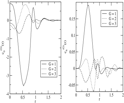
Figure 1: Harmonic coefficients $c_{M}^{(G)}(r)$ for RLV’s of first three sets. The full line represents values for the first set, the dotted line of the second set and dashed line of the third set. the distance r is in unit of $(\frac{1}{\rho})^{\frac{1}{2}}$ for a system of soft disks interacting via a reduced pair potential $\beta u(r)=\Gamma/r^{3}(\Gamma=12)$

In Fig.(1) we plot $c_{M}^{(G)}(r)$ which for a two- dimensional crystal is defined as 12

$$c^{(G)}(\vec{r})=\sum_{M}\>(i)^{M}\>c_{M}^{(G)}(\vec{r})\>e^{iM\phi_{G}}\>e^{-iM\phi_{r}}$$ (9)

where $M=0,\pm 6$ for a hexagonal lattice ,$\phi_{G}$ and $\phi_{r}$ are angles of vectors $\vec{G}$ and $\vec{r}$ with respect to a space fixed coordinate frame. The results given in the figure are for $\Gamma=12$ and found from the first term of (7). The values of ${c_{M}}^{(G)}$ is found to depend on values of order parameters $\rho_{G}$ and of RLVs. The values plotted are for RLVs of the first three sets. We see that for different set of $G$, ${c_{M}}^{(G)}(\vec{r})$ varies with $r$ in different way. The value becomes negligible for $r>1.5$ in all cases. For any given value of $G$, the value of ${c_{0}}^{(G)}(\vec{r})$ is about an order of magnitude higher than ${c_{6}}^{(G)}(\vec{r})$ at their maxima and minima. As the magnitude of $G$ increases, value of ${c_{M}}^{(G)}{(\vec{r})}$ decreases and after sixth set the value becomes negligible. As one goes at lower temperature/higher density more sets may contribute but the number will always remain few.

The usefulness of this method, however, depends on the convergence of the series (7). It has been shown in refs. 11 ; 12 that at the melting point $c^{(b)}$ is accurately approximated by the first term of (7). The following identity (see 17 ; 18 ), can be used to find contributions made by different terms of (7) and therefore its convergence :

$$\nabla_{1}\ln\rho({\roarrow{r}}_{1})=\int d{\roarrow{r}}_{2}c^{(0)}(|{\roarrow{r}}_{2}-{\roarrow{r}}_{1}|)+\sum_{G}\int d{\roarrow{r}}_{2}$$

$$\>\times[\nabla_{2}\rho({\roarrow{r}}_{2})+i(\rho({\roarrow{r}}_{2})-\rho)\vec{G}]e^{i\vec{G}\cdot{\roarrow{r}}_{c}}\tilde{c}^{(G)}({\roarrow{r}}_{2}-{\roarrow{r}}_{1}),$$ (10)

where, $\tilde{c}^{(b)}({\roarrow{r}})=\int^{1}_{0}d\xi\int^{1}_{0}d\lambda c^{(G)}({\roarrow{r}},\lambda\rho,\xi\rho_{G})$.

The l.h.s. of (10) is evaluated using $\rho({\roarrow{r}}_{1})=(\alpha/\pi)\sum_{i}\exp{[-\alpha({\roarrow{r}}-\vec{R_{i}})^{2}]}$ and the r.h.s. $\rho({\roarrow{r}})=\rho+\sum_{G}\mu_{G}\exp[-i\vec{G}\cdot{\roarrow{r}}]$ where $\rho_{G}=\rho\exp[-G^{2}/4\alpha]$. The value of $\alpha$ is taken 100 12 ; 19 . When values of $c^{(0)}(r)$ and of $c^{(G)}({\roarrow{r}})$ found from the first term of (7) are used, the r.h.s. of (10) gives values which are on the average $20\%$ higher than the values found from the l.h.s. This is an estimate of the contribution expected to come from higher order terms of (7), which as shown in ref 11 can be evaluated using the procedure describe above. We now proceed to calculate $h^{(b)}({\roarrow{r}}_{1},{\roarrow{r}}_{2})$.

Using (3) we can write (5) as (see 18 )

$$h^{(G)}(\vec{r})=\frac{1}{V}\sum_{k}H^{(G)}(\vec{k})e^{i\vec{k}\cdot{\roarrow{r}}}+\frac{\rho}{V}\sum_{G_{1}}\sum_{k}$$

$$\>h^{(G_{1})}\left(\vec{k}-\frac{1}{2}\vec{G}-\frac{1}{2}\vec{G_{1}}\right)\left[\mu_{G-G_{1}}c^{(0)}\left(-|\vec{k}+\frac{1}{2}\vec{G}|\right)\right.$$

$$\>\left.+\sum_{G_{2}}\mu_{G-G_{1}-G_{2}}c^{(G_{2})}\left(\frac{1}{2}\vec{G_{2}}-\frac{1}{2}\vec{G}-\vec{k}\right)\right]e^{i\vec{k}.\vec{r}},$$ (11)

where

$$H^{(G)}(\vec{k})=c^{(G)}(\vec{k})+\rho\>\mu_{G}\>c^{(0)}\left(|\vec{k}-\frac{1}{2}\vec{G}|\right)h^{(0)}\left(-|\vec{k}+\frac{1}{2}\vec{G}|\right)$$

$$\>+\rho\sum_{G_{1}}\mu_{G_{1}-G}\>c^{(G_{1})}\left(\vec{k}-\frac{1}{2}\vec{G}+\frac{1}{2}\vec{G_{1}}\right)h^{(0)}\left(-|\vec{k}+\frac{1}{2}\vec{G_{1}}|\right).$$ (12)

We adopt iterative method (see 18 ) to calculate values of $h^{(G)}({\roarrow{r}})$ from (11). It is found that the term that contains $c^{(G)}$ in (11) makes small contribution compared to the term that contains $c^{(0)}$, therefore some error in $c^{(G)}$ due to truncation of the series (7) will not affect the value of $h^{G}(r)$ in any significant way.

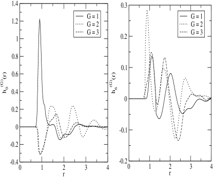
Figure 2: Harmonic coefficients $h_{M}^{(G)}(r)$ for RLV’s of first three sets. Notation are same as in Fig. 1

In Fig (2) we plot values of $h^{(G)}_{M}(r)$ defied as

$$h^{(G)}(\vec{r})=\sum_{M}(i)^{M}\>h^{(G)}_{M}(r)\>e^{iM\phi_{G}}\>e^{-iM\phi_{r}},$$ (13)

For the first three sets of $\vec{G}$ for $\Gamma=12$ and $\alpha=100$. The values of $h^{(G)}_{M}(r)$ depend on values of order parameters $\rho_{G}$ and on values of $\vec{G}$ vectors. For $G$ belonging to different sets, values of $h^{(G)}_{M}(r)$ as a function of $r$ oscillate about zero in different ways; the maxima and minima are located at different values of $r$. The values decay rapidly and become almost zero for $r>5$ in all cases. Unlike $c^{(G)}_{M}(r)$, the values of maxima and minima of $h^{(G)}_{0}(r)$ and $h^{(G)}_{6}(r)$ are comparable. As the magnitude of $G$ increases the value of $h^{(G)}_{M}(r)$ decreases and as in the case of $c^{(G)}_{M}(r)$ after sixth set the values become negligible.

The accuracy of $h^{(G)}(r)$ can be tested using a Ward identity which in this case is represented by the Born-Green -Yoven (YGB) equation 2 ,

$$\nabla_{1}\ln\rho(\vec{r}_{1}) =-\beta\int d\vec{r}_{2}\rho(\vec{r}_{2})(g^{(0)}(|\vec{r_{2}}-\vec{r}_{1}|)$$

$$\qquad+h^{(b)}(\vec{r}_{1},\vec{r}_{2}))\nabla_{1}u(|\vec{r}_{2}-\vec{r}_{1}|),$$ (14)

where $u(|\vec{r}_{2}-\vec{r}_{1}|)$ is the pair potential. It is solved to give

$$1=- \frac{\rho}{2\alpha r_{1}}\sum_{G}iJ_{1}(Gr_{1})\int d{\roarrow{r}}\left(\frac{\vec{G}}{|\vec{G}|}\cdot\frac{{\roarrow{r}}}{|{\roarrow{r}}|}\right)\frac{\delta(\beta u(r))}{\delta r}$$

$$\times\left[\mu_{G}g^{(0)}(r)e^{i\vec{G}\cdot{\roarrow{r}}}+h^{(G)}({\roarrow{r}})e^{\frac{1}{2}i\vec{G}\cdot{\roarrow{r}}}\right.$$

$$\left.+\sum_{G_{1}}\mu_{G-G_{1}}h^{(G_{1})}({\roarrow{r}})e^{i(\vec{G}-\frac{1}{2}\vec{G_{1}})\cdot{\roarrow{r}}}\right]$$ (15)

The values calculated for several values of $r_{1}$ are found to lie between $0.92-1.10$ indicating that the value of $h^{(G)}_{M}(r)$ given in Fig 2 are reasonably accurate.

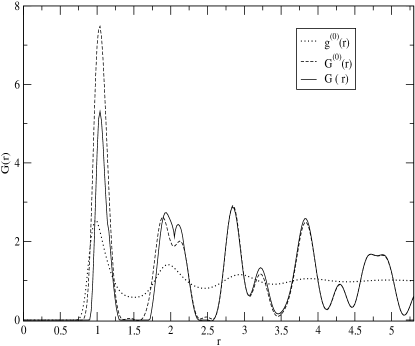
Figure 3: Correlation function $G(r)$ (see Eq. (16)) as a function of r. $G^{(0)}$ refers to values found without symmetry breaking part of $h({\roarrow{r}}_{1},{\roarrow{r}}_{2})$. $g^{(0)}(r)$ is the radial distribution function in a fluid of the average density of the crystal.

In computer simulations 20 and in experiments 21 $g(\vec{r}_{1},\vec{r}_{2})$ is reduced to a function of one variable,

$$G(r) =\frac{1}{\rho^{2}V}\int_{0}^{2\pi}\frac{d\phi_{r}}{2\pi}\int d\vec{r_{1}}\rho(\vec{r}_{1})\rho(\vec{r_{2}})$$

$$\qquad\times\left[g^{(0)}(|\vec{r_{2}}-\vec{r}_{1}|)+h^{(b)}(\vec{r_{1}},\vec{r}_{2})\right],$$ (16)

where $\phi_{r}$ is the angle of vector ${\roarrow{r}}={\roarrow{r}}_{2}-{\roarrow{r}}_{1}$. In the fluid $G(r)$ reduces to the radial distribution function $g^{(0)}(r)$. The values of $G(r)$ plotted in Fig (3) for $\Gamma=12$ as a function of r are in good qualitative agreement with the values found from simulations and experiments for soft colloidal particles 20 ; 21 ; as the pair potentials in these work are different we can not expect quantitative agreement. In the figure we also give the values of $g^{(0)}(r)$ and the value of $G^{(0)}(r)$ found without including the contribution of $h^{(b)}(\vec{r}_{1},\vec{r}_{2})$. It is seen that the effect of $h^{(b)}(\vec{r}_{1},\vec{r}_{2})$ is limited to the first two peaks of $G(r)$ only.

In conclusion; we developed a method to calculate PCFs in a crystal. This method is based on separating the correlation functions into the symmetry conserving and the symmetry broken parts. The symmetry conserving parts are calculated using the IET of homogeneous fluids. The symmetry broken part of $c(\vec{r}_{1},\vec{r}_{2})$ is calculated from a series written in powers of order parameters. The series involves three- and higher-body direct correlation functions of a homogeneous system which are calculated from relations connecting them with the density derivatives of $c^{(0)}(r,\rho)$ . It is shown that near the melting point most of the contribution comes from the first term of the series. As one goes deeper into the solid higher order terms may start contributing which can easily be calculated using the method used for the first term and described in 11 . The term $h^{(b)}(\vec{r}_{1},\vec{r}_{2})$ is calculated from the OZ equation using an iterative method. The values found for $h^{(G)}({\roarrow{r}})$ for $G$ of different sets differ substantively from each other, but in all cases they decay to zero for $r\geq 5$. This shows that $\rho(\vec{r}_{1})\rho(\vec{r}_{2})h(\vec{r}_{1},\vec{r}_{2})$ is a short range function. The accuracy of the values found for $h(\vec{r}_{1},\vec{r}_{2})$ has been examined using the YGB equation that relates $\rho(\vec{r}_{1})$ to the integral of $h(\vec{r}_{1},\vec{r}_{2})$. Fig 3 shows that it is the first two peaks of $G(r)$ which are mainly affected due to $h^{(G)}({\roarrow{r}})$ , this is due to mutual cancellations of values of different $G$ sets. Though the results reported here are for a two-dimensional solid, it is straightforward to apply the theory to three-dimensional crystals. On the basis of these results we conclude that the method proposed here can be used to obtain accurate and detailed informations about PCFs in crystals.

References

- (1) P. M. Chaikin and T. C. Lubensky, Principles of Condensed Matter Physics (Cambridge University Press, 1995).
- (2) J. P. Hansen and I. R. McDonald, Theory of Simple Liquids, 3rd ed (Academic press, Boston, 2006).
- (3) W. A. Curtin and N. W. Ashcroft, Phys. Rev. Lett. 56, 2775 (1986); Z Tang, L. E. Seriven and H. T. Davis, J Chem. Phys 95, 2659 (1991); S Sokolowski and J. Fischer, J. Chem. Phys. 96, 5441 (1992).
- (4) A. Kyrlidis and R. A. Brown, Phys. Rev. E 47, 427 (1993).
- (5) L. Mederas, G. Navascues and P. Tarazona, Phys. Rev. E 49, 2161 (1994); 47, 4284 (1993).
- (6) C. Rascon, L. Mederas, G. Navascues and P. Tarazona, Phys. Rev. Lett. 77, 2249 (1996).
- (7) R. F. Kayser, Jr., J.B. Hubbard and H. J. Raveche, Phys. Rev. B 24, 51 (1981).
- (8) J.S. McCarley and N. W. Ashcroft, Phys. Rev. E 55, 4990 (1997).
-
(9)
P. Mishra and Y. Singh, Phys. Rev. Lett. 97, 177801 (2006);
P. Mishra, S. L. Singh, J. Ram and Y. Singh, J. Chem. Phys. 127, 044905 (2007). -
(10)
S. L. Singh and Y. Singh, Europhys. Lett. 88, 16005 (2009)
S. L. Singh, A. S. Bharadwaj and Y. Singh, Phys. Rev. E 83, 051506 (2011). - (11) A. S. Bharadwaj, S. L. Singh and Y. Singh, Phys. Rev. E 88, 022112 (2013).
- (12) A. Jaiswal, S. L. Singh and Y. Singh, Phys. Rev. E 87, 012309 (2013).
- (13) Y. Singh, Phys. Rep. 207, 351 (1991).
- (14) F. J. Rogers and D. A. Young, Phys. Rev. A 30, 999 (1984).
- (15) K.Zahn, R. Lenke and G. Maret, Phys. Rev. Lett. 82, 2721 (1999); H. H. Grunberg, P. Keim, K. Zahn and G. Maret, Phys. Rev. Lett. 93 255703 (2004).
- (16) J. L. Barrat, J. P. Hansen and G. Pastore Mol. Phys. 63, 747 (1988); Phys. Rev. Lett. 58 2075 (1987).
- (17) R. Lovett, C. Y. Mou and F. P. Buff, J. Chem. Phys. 65, 570 (1976).
- (18) See Supplemental Material at
- (19) S. van Teeffelen, H. Lowen and C. N. Likos, J. Phys. Condens. Matter 20, 404217 (2008)
- (20) M. Antanger, G. Doppelbauer, M. Mazars and G. Kahl, J. Chem. Phys. 140, 044507 (2014).
- (21) Y. Han, N. Y. Ha, A. M. Alsayed, and A. G. Yodh, Phys. Rev. E 77, 041406 (2008).