Concise analytic solutions to the quantum Rabi model with two arbitrary qubits

Abstract

Using extended coherent states, an analytical exact study has been carried out for the quantum Rabi model (QRM) with two arbitrary qubits in a very concise way. The $G$-functions with $2\times 2$ determinants are generally derived. For the same coupling constants, the simplest $G$-function, resembling that in the one-qubit QRM, can be obtained. Zeros of the $G$-function yield the whole regular spectrum. The exceptional eigenvalues, which do not belong to the zeros of the $G$ function, are obtained in the closed form. The Dark states in the case of the same coupling can be detected clearly in a continued-fraction technique. The present concise solution is conceptually clear and practically feasible to the general two-qubit QRM and therefore has many applications.

1 Introduction

Quantum Rabi model (QRM) describes a two-level atom (qubit) coupled to a cavity electromagnetic mode (an oscillator) [1], a minimalist paradigm of matter-light interactions with applications in numerous fields ranging from quantum optics, quantum information science to condensed matter physics. The solutions to the QRM are however highly nontrivial. Whether an analytical exact solution even exists is uncertain for a long time. Recently, Braak presented an analytical exact solution [2] to the QRM using the representation of bosonic creation and annihilation operators in the Bargmann space of analytical functions [3]. A so-called $G$-function with a single energy variable was derived yielding exact eigensolutions, which is not in the closed form but well defined mathematically. Alternatively, using the method of extended coherent states (ECS), this $G$-function was recovered in a simpler, yet physically more transparent manner by Chen et al. [4]. Braak’s solution has stimulated extensive research interests in the single-qubit QRM [5].

As quantum information resources, such as the quantum entanglement [6] and the quantum discord [7], can be easily stored in two qubits, two qubits in a common cavity have potential applications in quantum information technology. Such a model system with two qubits now can be constructed in several solid devices [8, 9, 10]. Recently, some analytical studies to the QRM with two qubits have been attempted within various approaches [11, 12, 13, 14, 15, 16, 17]. By using the ECS technique, a $G$-function for the QRM with two equivalent qubits, resembling the simplest one without a determinant in the single-qubit QRM [2], was obtained [15]. While in the Bargmann representation, the $G$-function was built as a high order determinant, such as $8\times 8$ determinants for QRM with two different qubits [12, 13, 14].

Practically, the QRM with two arbitrary qubits is the most general one, and can be realized in experimental device with the greatest possibility. We believe that a simpler $G$-function is more convenient to obtain the eigensolutions, and can also shed light on many physical processes more clearly. In this work, employing the ECS, we demonstrate a successful derivation of a very concise $G$-function, which is just a $2\times 2$ determinant for the QRM with two arbitrary qubits. Furthermore, for the same coupling, the $G$-function even for two different qubits can be reduced to a simplest one without the use of the determinant, like that in the single-qubit QRM [2].

2 Analytical scheme to exact solutions

The Hamiltonian of the QRM with two qubits can be generally written as [12, 13, 14]

$$H={\omega}d^{{\dagger}}d+g_{1}\sigma_{1x}(d^{{\dagger}}+d)+g_{2}\sigma_{2x}\;(d^{{\dagger}}+d)+\Delta_{1}\sigma_{1z}+\Delta_{2}\sigma_{2z},$$ (1)

where $\Delta_{i}(i=1,2)$ is the energy splitting of the $i$-th qubit, $d^{{\dagger}}$ creates one photon in the common single-mode cavity with frequency $\omega$, $g_{i}$ describes the coupling strength between the $i$-th qubit and the cavity,    $\sigma_{ix}$ and $\sigma_{iz}~{}$ are the usual Pauli matrices of the $i$-th qubit. After a rotation with respect to the $y$-axis by an angle $\frac{\pi}{2},$ the Hamiltonian in the two-qubit basis $\left|1,1\right\rangle$, $\left|1,-1\right\rangle$, $\left|-1,1\right\rangle$, and $\left|-1,-1\right\rangle$, which are eigenstates of $\sigma_{1z}\otimes\sigma_{2z}$, can be written as the following symmetric matrix (in unit of $\omega=1$)

$$H=\left(\begin{array}[]{cccc}d^{{\dagger}}d+g\left(d^{{\dagger}}+d\right)&-\Delta_{2}&-\Delta_{1}&0\\ -\Delta_{2}&d^{{\dagger}}d+g^{\prime}\left(d^{{\dagger}}+d\right)&0&-\Delta_{1}\\ -\Delta_{1}&0&d^{{\dagger}}d-g^{\prime}\left(d^{{\dagger}}+d\right)&-\Delta_{2}\\ 0&-\Delta_{1}&-\Delta_{2}&d^{{\dagger}}d-g\left(d^{{\dagger}}+d\right)\end{array}\right),$$ (2)

where $g=g_{1}+g_{2}$ and $g^{\prime}=g_{1}-g_{2}$.

For later use, we express the wavefunction in terms of the Fock space as

$$\left|d\right\rangle=\sum_{n=0}^{\infty}\sqrt{n!}\left\{a_{n}\left[\left|1,1\right\rangle\pm\left(-1\right)^{n}\left|-1,-1\right\rangle\right]+b_{n}\left[\left|1,-1\right\rangle\pm\left(-1\right)^{n}\left|-1,1\right\rangle\right]\right\}|n\rangle,$$ (3)

where $+(-)$ corresponds to even (odd) parity, $\left|n\right\rangle\$is the photonic number state. The Schrödinger equation leads to the recurrence relation

$$a_{m+1} = \frac{\left[\Delta_{2}\pm\Delta_{1}\left(-1\right)^{m}\right]b_{m}-\left(m-E\right)a_{m}-ga_{m-1}}{g\left(m+1\right)},$$

$$b_{m+1} = \frac{\left[\Delta_{2}\pm\Delta_{1}\left(-1\right)^{m}\right]a_{m}-\left(m-E\right)b_{m}-g^{\prime}b_{m-1}}{g^{\prime}\left(m+1\right)}.$$ (4)

Note that they cannot be reduced to a linear three-term recurrence form. The coefficients $a_{n},b_{n}$ can be obtained in terms of two initial values of $a_{0}$ and $b_{0}$ recursively.

In this paper, we will first study the general case of different coupling strengths with the same cavity, then we turn to the special equal coupling case.

2.1 Two-qubit QRM for $g_{1}\neq g_{2}$

To employ the ECS approach, we first perform the following pair of Bogoliubov transformations with finite displacements

$$A_{+}^{\dagger} = d^{\dagger}+g,\;A_{-}^{\dagger}=d^{\dagger}-g;$$ (5)

$$B_{+}^{\dagger} = d^{\dagger}+g^{\prime},\;B_{-}^{\dagger}=d^{\dagger}-g^{\prime},$$ (6)

by which some diagonal matrix element   can be reduced to the free particle number operators plus a constant, which is very helpful for the further study.

The wavefunction can be expanded in the Fock space of the operator $A_{+}^{\dagger}$

$$|A_{+}\rangle=\sum_{n=0}^{\infty}\sqrt{n!}\left[u_{n}^{A}\left|1,1\right\rangle+z_{n}^{A}\left|-1,-1\right\rangle+v_{n}^{A}\left|1,-1\right\rangle+w_{n}^{A}\left|-1,1\right\rangle\right]|n\rangle_{A_{+}},$$ (7)

where$\;|n\rangle_{A_{+}}\;$is the number state in the $A_{+}^{\dagger}$-space, and termed as the ECS previously [19]. The Schrödinger equation straightforwardly gives

$$u_{m}^{A} = \frac{\Delta_{2}v_{m}^{A}+\Delta_{1}w_{m}^{A}}{m-E-g^{2}},$$

$$v_{m+1}^{A} = -\frac{\Delta_{1}z_{m}^{A}+\Delta_{2}u_{m}^{A}-\left(m-E+g^{2}-2gg^{\prime}\right)v_{m}^{A}}{\left(m+1\right)\left(g-g^{\prime}\right)}-\frac{v_{m-1}^{A}}{m+1},$$

$$w_{m+1}^{A} = -\frac{\Delta_{2}z_{m}^{A}+\Delta_{1}u_{m}^{A}-\left(m-E+g^{2}+2gg^{\prime}\right)w_{m}^{A}}{\left(g+g^{\prime}\right)\left(m+1\right)}-\frac{w_{m-1}^{A}}{\left(m+1\right)},$$

$$z_{m+1}^{A} = -\frac{\Delta_{1}v_{m}^{A}+\Delta_{2}w_{m}^{A}-\left(m-E+3g^{2}\right)z_{m}^{A}}{2g\left(m+1\right)}-\frac{z_{m-1}^{A}}{\left(m+1\right)},$$ (8)

which cannot be reduced to the linear three-term recurrence relation either. Note that if three initial coefficients $v_{0}^{A},w_{0}^{A},z_{0}^{A}$ are given, all other coefficients will be uniquely determined recursively.

Considering the conserved parity, the wavefunction can be also expressed in series expansion in the Fock space of $A_{-}^{\dagger}$

$$\left|A_{-}\right\rangle=\sum_{n=0}^{\infty}(-1)^{n}\sqrt{n!}\left[z_{n}^{A}\left|1,1\right\rangle+u_{n}^{A}\left|-1,-1\right\rangle+w_{n}^{A}\left|1,-1\right\rangle+v_{n}^{A}\left|-1,1\right\rangle\right]|n\rangle_{A_{-}}.$$

The wavefunction for non-degenerate state should be the same, so we have

$$\sum_{n=0}^{\infty}\sqrt{n!}u_{n}^{A}|n\rangle_{A_{+}}=r\sum_{n=0}^{\infty}(-1)^{n}\sqrt{n!}z_{n}^{A}|n\rangle_{A_{-}};\;\;\sum_{n=0}^{\infty}\sqrt{n!}z_{n}^{A}|n\rangle_{A_{+}}=r\sum_{n=0}^{\infty}(-1)^{n}\sqrt{n!}u_{n}^{A}|n\rangle_{A_{-}}.$$

Projecting onto $\langle 0|$ and with the use of $\sqrt{n!}\left\langle 0\right||n\rangle_{A_{+}}=(-1)^{n}\sqrt{n!}\left\langle 0\right||n\rangle_{A_{-}}=e^{-g^{2}/2}(g)^{n}$, we have one linear equation

$$G_{\pm}^{A}=\sum_{n=0}^{\infty}\left[u_{n}^{A}\mp z_{n}^{A}\right]g^{n}=0,$$ (9)

where $+(-)$ in left-hand-side is for even (odd) parity.

We can also expand the wavefunction in the Fock space of the second displaced operators $B_{+}^{\dagger}$

$$\left|B_{+}\right\rangle=\sum_{n=0}^{\infty}\sqrt{n!}\left[u_{n}^{B}\left|1,1\right\rangle+z_{n}^{B}\left|-1,-1\right\rangle+v_{n}^{B}\left|1,-1\right\rangle+w_{n}^{B}\left|-1,1\right\rangle\right]|n\rangle_{B_{+}}.$$ (10)

The Schrödinger equation yields

$$u_{m+1}^{B} = -\frac{\Delta_{2}v_{m}^{B}+\Delta_{1}w_{m}^{B}-\left(m-E+g^{\prime 2}-2g^{\prime}g\right)u_{m}^{B}}{\left(m+1\right)\left(g^{\prime}-g\right)}-\frac{u_{m-1}^{B}}{m+1},$$

$$v_{m}^{B} = \frac{\Delta_{1}z_{m}^{B}+\Delta_{2}u_{m}^{B}}{\left(m-E-g^{\prime 2}\right)},$$

$$w_{m+1}^{B} = -\frac{\Delta_{2}z_{m}^{B}+\Delta_{1}u_{m}^{B}-\left(m-E+3g^{\prime 2}\right)w_{m}^{B}}{2g^{\prime}\left(m+1\right)}-\frac{w_{m-1}^{B}}{\left(m+1\right)},$$

$$z_{m+1}^{B} = -\frac{\Delta_{1}v_{m}^{B}+\Delta_{2}w_{m}^{B}-\left(m-E++g^{\prime 2}+2g^{\prime}g\right)z_{n}^{B}}{\left(m+1\right)\left(g+g^{\prime}\right)}-\frac{z_{m-1}^{B}}{\left(m+1\right)}.$$ (11)

All coefficients for $m>0$ can be determined from three initial parameters $u_{0}^{B},w_{0}^{B},z_{0}^{B}$ recursively. Through the similar procedure, we can obtain the second linear equation as

$$G_{\pm}^{B}=\sum_{n=0}^{\infty}\left[v_{n}^{B}\mp w_{n}^{B}\right](g^{\prime})^{n}=0.$$ (12)

There seems to be $6$ initial coefficients in Eqs. (9) and (12). Fortunately, they can be determined by coefficients in the series expansion Eq. (3) in the original Fock space. For example, the same wavefunction for non-degenerate states implies $|A_{+}\rangle\varpropto|d\rangle$. Projecting onto ${}_{A+}\langle 0|$ yields

$$v_{0}^{A}=\sum_{n=0}^{\infty}b_{n}\;\left(-g\right)^{n};\;w_{0}^{A}=\pm\sum_{n=0}^{\infty}b_{n}g^{n};z_{0}^{A}=\pm\sum_{n=0}^{\infty}a_{n}g^{n},$$ (13)

where we have used ${}_{\ A_{+}}\langle 0|n\rangle=\sqrt{\frac{1}{n!}}e^{-g^{2}/2}\left(-g\right)^{n}$, and removed irrelevant constants. Then we can obtain $u_{n}^{A}\;$and$\;z_{n}^{A}$ in Eq. (9) through Eq. (8) recursively. Similarly, $v_{0}^{B},w_{0}^{B},z_{0}^{B}$ can also be obtained by coefficients $a_{n}$ and $b_{n}$. Through Eq. (11), we can get all $v_{n}^{B}$ and $w_{n}^{B}$ in Eq. (12).

Inserting these coefficients into Eqs. (9) and (12), we can arrive at two linear equations for $a_{0}$ and $b_{0}$

$$G_{11}a_{0}+G_{12}b_{0} = 0,$$

$$G_{21}a_{0}+G_{22}b_{0} = 0,$$

where $G_{11}\;$and $G_{21}$ are obtained from Eqs. (9) and (12)  by setting $a_{0}=1$ and $b_{0}=0$ ; $G_{12}\;$and $G_{22}\;$are obtained by setting $a_{0}=0$ and $b_{0}=1$. The $G$-function is then defined with the following $2\times 2$ determinant

$$G_{\pm}(E)=\left|\begin{array}[]{ll}G_{11}&G_{12}\\ G_{21}&G_{22}\end{array}\right|=0.$$ (14)

Nonzero coefficients require the vanishing $G$-function in the real physics problems. So the zeros of this $G$-function will give the energy spectrum for the present model. In addition, from the first one in Eq. (8) and the second one in Eq. (11), we immediately know that $E_{ex}^{(1)}=m-g^{2}$ and $E_{ex}^{(2)}=m-(g^{\prime})^{2}$ are two sets of the exceptional solutions, which are not the zeros of the $G$-function. It is interesting to note from the coefficients in Eqs. (8), (11), and (13) that the present $G$-function is a well defined transcendental function. Thus analytical exact solutions have been formally found.

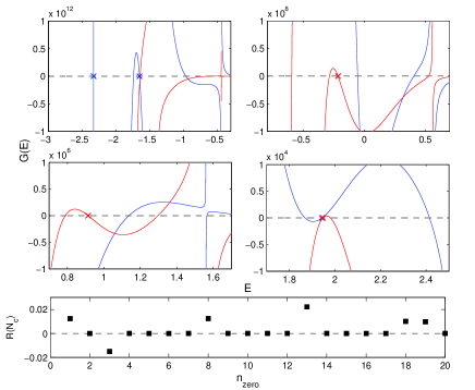
Figure 1: (Color online) (upper and middle panels) $G$-functions for the two-qubit QRM with even (blue) and odd (red) parity using different scales in four energy intervals connected successively. Crosses denote the unstable zeros. (Bottom) $R_{N_{c}}=\ln\left(E_{N_{c}}/E_{N_{c}+1}\right)$ for different zeros with the serial number $n_{zero}$. $\Delta_{1}=0.7$, $\Delta_{2}=0.4$ and $g_{1}=2g_{2}=0.8$.

We plot the $G$-function for $\Delta_{1}=0.7,$ $\Delta_{2}=0.4\;$and $g_{1}=2g_{2}=0.8\;$ in Fig. 1. The stable zeros reproduce all regular spectra, which can be confirmed by the numerical exact solutions. Typically, the convergence is assumed to be achieved if zeros (i.e. $E$) are determined within relative errors $\left|\left(E_{N_{c}}-E_{N_{c}+1}\right)/E_{N_{c}+1}\right|<10^{-8}$, where $N_{c}$ is the truncated number of the series expansions in the space of the displaced operators. We also calculate $R_{N_{c}}=\ln\left(E_{N_{c}}/E_{N_{c}+1}\right)$ for all zeros, which are exhibited in Fig. 1 (b). For the stable zeros, $R_{N_{c}}$ is almost the same as the relative errors and should be around the $R_{N_{c}}=0$ line within error $10^{-8}$, much smaller than the symbol size.

While, very few unstable zeros, which are not the true eigenvalues, are also present in practical calculations because of unavoidable finite truncations. Fortunately, they can be excluded very easily. They are very sensitive to the truncated number $N_{c}$ and cannot converge with increasing $N_{c}$, because the corresponding coefficients oscillate with increasing magnitudes as $n$ increases. In sharp contrast, for the stable zeros, the coefficients converges to zero rapidly with $n$. The positions of unstable zeros must change even increasing $N_{c}$ by $1$. So they can be easily figured out in Fig. 1 (b) for apparent deviation from $R_{N_{c}}=0$ line. It should be pointed out here that these unstable zeros are absolutely not the true zeros of $G$-function, and will disappear if the summations are really performed infinitely.

The baselines shown in Fig. 1 (a) are close to $E_{ex}^{(1)}$ and $E_{ex}^{(2)}$ exceptional eigenvalues due to the divergence in the $G$-functions. Generally, the exceptional eigenvalues hardly occur for given rational model parameters.

It is interesting to note that the present $G$-function within ECS is only a $2\times 2$ determinant, much simpler than those with $8\times 8$ determinants in the same model using the Bargmann representation [14].

2.2 Two-qubit QRM for $g_{1}=g_{2}$

For the same coupling, $g^{\prime}=0,$ the Hamiltonian matrix (2) is of higher symmetry due to $H_{22}=H_{33}$, the solution will become simpler. The wavefunction in the series expansion in the original Fock space is the same as Eq. (3), but the recurrence relation obtained from the Schrödinger equation should take a simpler form

$$\left[\Delta_{2}\pm\Delta_{1}\left(-1\right)^{m}\right]a_{m} = \left(m-E\right)b_{m},$$ (15)

$$\left[\Delta_{2}\pm\Delta_{1}\left(-1\right)^{m}\right]b_{m} = \left(m-E\right)a_{m}+g\left[a_{m-1}+\left(m+1\right)a_{m+1}\right].$$

Note that one-to-one relation of $a_{m}\;$and $b_{m}\;$is found, and thus a three-term recurrence relation can be obtained, in contrast with the case of $g_{1}\neq g_{2}$. The coefficients can be obtained in terms of only one initial value $b_{0}=1$ or $a_{0}=1$ recursively, so the continued-fraction technique is directly applicable, similar to that in the single-qubit QRM [18]. We can choose initial parameter $b_{0}=1$ for $\Delta_{2}\neq\Delta_{1}$,   and $a_{0}=1\;$for $\Delta_{2}=\Delta_{1}$ to avoid the artificial divergence.

Alternatively, we propose a mathematically well-defined technique. The wavefunction can be expressed as Eq. (7) in terms of the sole pair of the displaced operators $A$ in Eq. (5). Set $y_{m}=\Delta_{2}v_{m}^{A}+\Delta_{1}w_{m}^{A}$, Eq. (8) can be reduced to the following recurrence relation

$$u_{m}^{A} = \frac{y_{m}}{m-E-g^{2}},$$

$$y_{m+1} = -\frac{2\Delta_{2}\Delta_{1}z_{m}^{A}+\left(\Delta_{1}^{2}+\Delta_{2}^{2}\right)u_{m}^{A}-\left(m-E+g^{2}\right)y_{m}}{\left(m+1\right)g}-\frac{y_{m-1}}{m+1},$$

$$z_{m+1}^{A} = -\frac{y_{m}-\left(m-E+3g^{2}\right)z_{m}^{A}}{2g\left(m+1\right)}-\frac{z_{m-1}^{A}}{\left(m+1\right)}.$$ (16)

Although they cannot be reduced to a linear three-term relation either, the coefficients can be uniquely given recursively by only two initial coefficients $y_{0}^{A}$ and $z_{0}^{A}$ in this case. To this end, we can define the $G$-function as

$$G_{\pm}=\sum_{n=0}^{\infty}\left[u_{n}^{A}\mp z_{n}^{A}\right]g^{n}=0.$$ (17)

Next we need build the relationship between two sets of coefficients for series expansions in $d$ and $A$. For the same wavefunction, we have

$$\sum_{n=0}^{\infty}\sqrt{n!}y_{n}^{A}|n\rangle_{A_{+}}=r\sum_{n=0}^{\infty}\sqrt{n!}\left[\Delta_{2}\pm\Delta_{1}\right]b_{n}|n\rangle,\;\sum_{n=0}^{\infty}\sqrt{n!}z_{n}^{A}|n\rangle_{A_{+}}=\pm r\sum_{n=0}^{\infty}\left(-1\right)^{n}\sqrt{n!}a_{n}|n\rangle.$$

Projecting onto ${}_{A+}\langle 0|$ yields

$$y_{0}^{A}=\pm\sum_{n=0}^{\infty}\left(\Delta_{2}\pm\Delta_{1}\right)b_{n}g^{n},z_{0}^{A}=\pm\sum_{n=0}^{\infty}a_{n}g^{n}.$$

Both $y_{0}^{A}$ and $z_{0}^{A}$ are determined by coefficients $a_{n}$ and $b_{n}$, which are only dependent on the initial parameter. Hence $u_{n}^{A}$ and $z_{n}^{A}$ in Eq. (17 ) can be obtained recursively from Eq. (16). Thus for the QRM of two different qubits but with the same coupling, we have derived the simplest $G$-function without the use of the determinant, similar to that in the one-qubit QRM [2, 4]. Note that the $G$-function in this case in Ref. [14] is a $4\times 4$ determinant.

Similarly, we also plot the $G$-function for $\Delta_{1}=0.7,$ $\Delta_{2}=0.4$ and $g_{1}=g_{2}=0.4$ in Fig. 2. The stable zeros give all eigenvalues and the unstable zeros can be distinguished by the same trick outlined above.

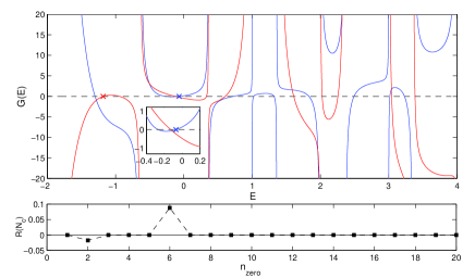
Figure 2: (Color online) (upper) $G$-functions for the two-qubit QRM with the same coupling constants with even (blue) and odd (red) parity. Crosses denote the unstable zeros. (Bottom) $R_{N_{c}}=\ln\left(E_{N_{c}}/E_{N_{c}+1}\right)$ for different zeros with the serial number $n_{zero}$. $g_{1}=g_{2}=0.4$ and $\Delta_{1}=0.7,\Delta_{2}=0.4$.

From Eq. (16), we know that $E=m-g^{2}$ is an exceptional solution. However, $E=m$ is neither an exceptional solution nor a singularity for    $\Delta_{1}\neq\Delta_{2}$, in contrast with the previous observation [14]. We attribute the difference to the possible enlarged dimension where their G function is defined. The final results should be the same in both kinds of treatments, but the present scheme is much more concise and allows an in-depth discussion.

By Eq. (15) we may write the recurrence relation as

$$g\left(m+1\right)a_{m+1}=\frac{\left[\Delta_{2}\pm\Delta_{1}\left(-1\right)^{m}\right]^{2}}{\left(m-E\right)}a_{m}-\left(m-E\right)a_{m}-ga_{m-1}.$$ (18)

For $\Delta_{2}=\Delta_{1}=\Delta$, the analyticity of the wave function requires $E=m$ for the even $m$ for odd parity and odd $m$ for even parity, independent of the coupling strength $g$. It is just the trivial eigenvalue for the spin-singlet state.

For $\Delta_{1}\neq\Delta_{2}$, the first two coefficients for the states with even parity are

$$a_{1}=-\frac{1}{g}\left[\left(\Delta_{2}+\Delta_{1}\right)^{2}-1\right]a_{0};\;a_{2}=\lim_{E\rightarrow 1}\frac{1}{2g}\left[\frac{a_{1}}{E-1}\left(\Delta_{2}-\Delta_{1}\right)^{2}-ga_{0}\right].$$

The non-analyticity of the eigenfunction only occurs for the possible divergence of $a_{2}$ where the denominator is zero. To lift the pole of $a_{2}$, it is required that $a_{1}=0$, which immediately yields

$$\left(\Delta_{2}+\Delta_{1}\right)^{2}=1.$$ (19)

While the first two coefficients for states with odd parity are

$$a_{1}=-\frac{1}{g}\left[\left(\Delta_{2}-\Delta_{1}\right)^{2}-1\right]a_{0};\;a_{2}=\lim_{E\rightarrow 1}\frac{1}{2g}\left[\frac{a_{1}}{E-1}\left(\Delta_{2}+\Delta_{1}\right)^{2}-ga_{0}\right].$$

The analyticity of $a_{2}\;$requires $a_{1}=0,$ which gives

$$\left(\Delta_{2}-\Delta_{1}\right)^{2}=1.$$ (20)

Equations (19) and (20) are just the conditions for special Dark states with $E=1$ found by Peng et al., [14]. So they can be easily figured out in the continued-fraction technique.

Figure 3: (Color online) The energy levels for the two-qubit QRM as a function of the coupling $g=2g_{1}=2g_{2}$. (left) $\Delta_{1}=0.7,$ $\Delta_{2}=0.3$; (right) $\Delta_{1}=1.3$ $\Delta_{2}=0.3$. $E=m$ denoted by dashed lines.

Figure 3 presents the energy spectra for two sets of $\Delta_{1}$, $\Delta_{2}$, which satisfy Eqs. (19) and (20) respectively. It is shown clearly that $E=1$ for $\Delta_{1}+\Delta_{2}=1$ and $\Delta_{1}-\Delta_{2}=1$ are $g$ independent eigenvalues for even and odd parity respectively. The states with $E=m\neq 1$ are not the dark states, which are exhibited obviously in Fig. 3.

3 Summary and discussion

In this work, we have derived the concise $G$-function for the QRM with two arbitrary qubits by using ECS, which leads to simple, analytic solutions. Although the coefficients in the recurrence relations look complicated, actually they can be uniquely and straightforwardly given by the Schrödinger equations. Our $G$-function is only a $2\times 2$ determinant for the general case and a rather simple one without a determinant for the same coupling case, much more concise than those derived recently in the Bargmann space. This work is to extend the methodology of a compact $G$-function in the QRM with one qubit to the QRM with two arbitrary qubits in the simplest way, thereby allowing a conceptually clear, practically feasible treatment to energy spectra. It is our expectation that the present concise approach will find more applications in the future.

We stress that the present analytic solution is well defined mathematically, because of no built-in truncations, which is essentially different from the previous finite truncation approaches [11, 16, 17] and the continued-fraction technique, therefore of both fundamental and practical interest.

ACKNOWLEDGEMENTS

QHC acknowledge useful discussions with Daniel Braak and Jie Peng. This work was supported by National Natural Science Foundation of China under Grant No. 11174254, National Basic Research Program of China under Grant No. 2011CBA00103.

^∗ Corresponding author. Email:qhchen@zju.edu.cn

References

References

• [1] I. I. Rabi, Phys. Rev. 49 (1936)324 ; 51 (1937)652.
• [2] D. Braak, Phys. Rev. Lett. 107 (2011)100401.
• [3] V. Bargmann, Comm. Pure Appl. Math. 14 (1961)197 .
• [4] Q. H Chen, C. Wang, S. He, T. Liu, and K. L. Wang, Phys. Rev. A 86 (2012)023822.
• [5] A. Moroz, Europhys. Lett. 100 (2012)60010 ; I. Travenec, Phys. Rev. A 85 (2012)043805; B. Gardas, J. Dajka, J. Phys. A 46 (2013)265302 ; Y. Z. Zhang, J. Phys. A 54 (2013)102104; A. J. Maciejewski, M. Przybylska, T. Stachowiak, Phys. Lett. A 378 (2014)3445; H. H. Zhong et al., J. Phys. A 46 (2013)415302; inbid 47 (2014)045301.
• [6] M. A. Nielsen and I. L. Chuang, Quantum Computation and Quantum Information (Cambridge University Press, Cambridge, England, 2000).
• [7] H. Ollivier and W. H. Zurek, Phys. Rev. Lett. 88 (2001)017901; W. H. Zurek, Phys. Rev. A 67 (2003)012320 .
• [8] M. A. Sillanpaa, J. I. Park, and R. W. Simmons R W, Nature 449 (2007)438; G. Haack, F. Helmer, M. Mariantoni, F. Marquardt and E. Solano, Phys. Rev. B 82 (2010)024514; F. Altintas and R. Eryigit, Phys. Lett. A 376 (2012)1791.
• [9] J. Benhelm, G. Kirchmair, C. F. Roos, and R. Blatt, Nature Phys. 4 (2008)463 ; C. A. Ryan, M. Laforest, and R. Laflamme, New J. Phys. 11 (2009)013034 ; A. D. Corcoles, Phys. Rev. A 87 (2013)030301.
• [10] L. DiCarlo et al., Nature 460,(2009)240 ; M. Neeley et al., Nature 467 (2010)570 ; R. Barends et al., Nature 508,(2014)500.
• [11] S. Agarwal, S. M. Hashemi Rafsanjani, and J. H. Eberly, Phys. Rev. A 85 (2012)043815 .
• [12] S. A. Chilingaryan and B. M. Rodriguez-Lara, J. Phys. A. : Math. Theor 46 (2013)335301.
• [13] B. M. Rodriguez-Lara, J. Phys. A: Math. Theor. 47 (2014)135306.
• [14] J. Peng et al. J. Phys. A: Math. Theor. 47 (2014)265303 .
• [15] H. Wang, S. He, L. W. Duan, and Q. H. Chen, EPL 106 (2014)54001.
• [16] L. J. Mao, S. N. Huai, Y. B. Zhang, arXiv:1403.5893 (2014).
• [17] Y. Y. Zhang and Q. H. Chen, arXiv:1410.1965(2014).
• [18] S. Swain, J. Phys. A 6 (1973)1919 .
• [19] Q. H. Chen, Y. Y. Zhang, T. Liu, and K. L. Wang, Phys. Rev. A 78 (2008) 051801(R) ; T. Liu, Y. Y. Zhang, Q. H. Chen, and K. L. Wang, Phys. Rev. A 80 (2009) 023810.