Effective orbital ordering in multiwell optical lattices with fermionic atoms

Abstract

We consider the behavior of Fermi atoms on optical superlattices with two-well structure of each node. Fermions on such lattices serve as an analog simulator of Fermi type Hamiltonian. We derive a mapping between fermion quantum ordering in the optical superlattices and the spin-orbital physics developed for degenerate $d$-electron compounds. The appropriate effective spin-orbital model appears to be the modification of the Kugel-Khomskii Hamiltonian. We show how different ground states of this Hamiltonian correspond to particular spin-pseudospin arrangement patterns of fermions on the lattice. The dependence of fermion arrangement on phases of complex hopping amplitudes is illustrated.

I Introduction

Experimental investigations of ultracold atoms in optical lattices have opened up a unique flexibly tunable simulator for study of quantum many-body physics Greiner et al. (2002); Köhl et al. (2005); Kawaguchi and Ueda (2012); Hauke et al. (2012) in the parameter range that had been hardly possible or even impossible to achieve in the natural solid state systems Meacher (1998); Jaksch et al. (1998); Grimm et al. (2000); Corboz et al. (2012).

Atom temperature on the optical lattice can be made extremely low. It opens the experimental way to investigate in detail the structure of the ground state and the low-lying many-body states of atoms Bloch et al. (2008); Quéméner and Julienne (2012). One of the most interesting regimes corresponds to the strong atom-atom quantum correlations. Interactions between atoms on the lattice have different nature. Atoms can jump (tunnel) from site to site of the optical lattice with the characteristic hoping energy $t$. Within the site typically there is repulsion $U$ between atoms. While the atoms have spins there is exchange interaction between the spins of the atoms on the neighboring sites of the lattice. The quantum state of the atoms on the lattice also strongly depends on the statistics of atoms, either they are bosons or fermions Lewenstein et al. (2007). In what follows we shall focus on the fermion case.

Typically atoms on the lattice could be well described by modifications of the Hubbard model due to the short-range character of the atom-atom interaction $U$ Jaksch et al. (1998). The problem of the ground state and the low-lying many-body states of atoms on the lattice have been successfully investigated within the mean-field theory, see e.g. Ref. Lewenstein et al., 2007. Progress have also been made beyond the mean-field theory in particular with numerical simulations of the Hubbard-type models. For bosons on the lattice parameter range of $U$ and $t$ at which one could expect Bose-condensation or the Mott-insulator behavior was thoroughly investigated Lewenstein et al. (2007); Wagner et al. (2011). Experimental realization of a Mott insulator regime of fermions on the optical lattice Jördens et al. (2008) opened a unique possibility to simulate various ground states and spin orderings of fermions, complying with theoretical predictions for the repulsive Fermi-Hubbard model.

Recently optical lattices with complicated structure of the node attracted much attention, in particular, superlattices with two-well structure Anderlini et al. (2007a); Fölling et al. (2007); Anderlini et al. (2007b); Trotzky et al. (2008); Wagner et al. (2012). The mean-field ground-state phase diagram of spinor bosons in two-well superlattice was found using Bose-Hubbard Hamiltonian in Ref. Wagner et al., 2012. It was shown that the system supports Mott-insulating as well as superfluid phases like in one-well latices. But the quadratic Zeeman effect lifts the degeneracy between different polar superfluid phases leading to additional metastable phases and first-order phase transitions.

Here we focus our study on spinor fermions on optical superlattices with multi-well structure of each node. Specifically, we consider two-well nodes in the regime of strong correlations (large $U/t$). We show how the ground many-body atom state on the lattice can be understood without direct solving of the Hubbard model but using the well known results of the machinery developed long ago for degenerate $d$-electron compounds Kugel and Khomskii (1973); Kugel’ and Khomskii (1982). We show that there is a mapping between fermion quantum ordering in the optical superlattices and the spin-orbital physics of degenerate $d$-electron compounds. We derive the effective spin-orbital model and show that it appears to be the generalization of the Kugel-Khomskii Hamiltonian Kugel and Khomskii (1973). Different ground states of this Hamiltonian correspond to particular nontrivial fermion arrangement on the lattice.

The paper is organized as follows: In the beginning of Sec. II we write down the Hubbard-type Hamiltonian for fermions on multi-well lattice. Then in Sec. II.2 more or less standard steps have been done to reduce the model to the effective spin-orbital Hamiltonian. Some rather cumbersome technical details of the reduction we put in the Appendix. In the Discussions, Sec. III, we give examples of possible atom many-body ground states on the lattice that can be obtained from the mapping to orbital-spin physics.

II Microscopic model for the fermions in the double-well optical lattice

II.1 Tunnel Hamiltonian model

We consider the $d$-dimensional hypercube optical lattice where each node is a double well, as is illustrated for the two-dimensional lattice in Fig. 1.

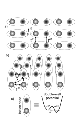
Figure 1: a,b) The sketch of possible optical lattices with two-well structure where spin-orbital effects may show up. $t^{\alpha\beta}$ are hopping amplitudes between wells on nearest nodes. Indices $\alpha,\beta=1,2$ numerate the two wells at a given lattice node (two quantum pseudospin states). c) The structure of the lattice node. $\Delta^{z}$ is the energy offset between the two wells.

The Hamiltonian describing the quantum states of fermions on the lattice can be written as

$$H=H_{\Delta}+\operatorname{\mathit{H}_{\mathrm{\scriptscriptstyle T}}}+\operatorname{\mathit{H}_{\mathrm{\scriptscriptstyle U}}}+\operatorname{\mathit{H}_{\mathrm{\scriptscriptstyle J}}}.$$ (1)

The term $H_{\Delta}$ describes the level structure of each node

$$H_{\Delta}=\sum_{i,\sigma,\alpha,\beta}\frac{1}{2}\left(\Delta_{i}^{z}\sigma^{z}_{\alpha\beta}+\Delta_{i}^{x}\sigma^{x}_{\alpha\beta}\right){\,}c^{\dagger}_{i\alpha\sigma}c_{i\beta\sigma},$$ (2)

where index $i$ labels the nodes, $\alpha=1,2$ is the well number at a given node, $\Delta_{i}^{z}$ is the difference of the ground state energies between the two wells, while $\Delta_{i}^{x}$ takes into account possible tunneling between the wells in a node. $\sigma^{z}$ and $\sigma^{x}$ are Pauli matrices. Operator $c^{{\dagger}}_{i\alpha\sigma}(c_{i\alpha\sigma})$ is the fermion creation (annihilation) operator for fermion atom residing at a node $i$, in a well $\alpha$ with spin projection $\sigma$.

Tunneling between the nodes specifies

$$\operatorname{\mathit{H}_{\mathrm{\scriptscriptstyle T}}}=-\sum_{i\neq j,\sigma,\alpha,\beta}t_{ij}^{\alpha\beta}c^{\dagger}_{i\alpha\sigma}c_{j\beta\sigma},$$ (3)

where $t_{ij}^{\alpha\beta}$ is the tunnel matrix element. The structure of the tunnel matrix elements is schematically depicted in Fig. 1a,b. The hopping amplitudes $t_{ij}^{\alpha\beta}$ can be arranged into complex-valued amplitude matrix in the well-space:

$$t_{ij}^{\alpha\beta}=t^{\alpha\beta}=\begin{pmatrix}t^{11}&t^{12}\\ t^{21}&t^{22}\end{pmatrix}.$$ (4)

We shall omit for brevity the lattice indices in hopping amplitudes. Below notation $t^{\dagger}=t^{\dagger}_{ij}$ will be used for the Hermitian conjugation in the well-subspace. Note that, in general, $t\neq t^{\dagger}$. Due to the Hermitian character of $\operatorname{\mathit{H}_{\mathrm{\scriptscriptstyle T}}}$ there is a standard symmetry, $t_{ij}^{\alpha\beta}=(t_{ji}^{\beta\alpha})^{*}$. It follows that $t^{\dagger}$ corresponds to the hopping amplitude matrix with interchanged lattice indices, i.e. $(t^{\dagger})^{\alpha\beta}=(t_{ij}^{\beta\alpha})^{*}=t_{ji}^{\alpha\beta}$.

Since each node has the “fine” structure related to the wells it is convenient to split the interaction Hamiltonian into two parts, $\operatorname{\mathit{H}_{\mathrm{\scriptscriptstyle U}}}+\operatorname{\mathit{H}_{\mathrm{\scriptscriptstyle J}}}$. The first term has a trivial structure in the well index space, and describes the Coulomb repulsion $(U_{i}>0)$ of fermions at one node:

$$\operatorname{\mathit{H}_{\mathrm{\scriptscriptstyle U}}}=\sum_{i,\sigma,\sigma^{\prime},\alpha,\alpha^{\prime}}U_{i}n_{i\alpha\sigma}n_{i,\alpha^{\prime},\sigma^{\prime}}(1-\delta_{\alpha\alpha^{\prime}}\delta_{\sigma\sigma^{\prime}}),$$ (5)

where $n_{i\alpha\sigma}=c^{\dagger}_{i\alpha\sigma}c_{i\alpha\sigma}$. The second term describes the ferromagnetic Hund’s coupling Kugel’ and Khomskii (1982) $(\operatorname{\mathit{J}_{\mathrm{\scriptscriptstyle H}}}^{(i)}>0)$ between fermions in wells $\alpha=1$ and 2 at a given lattice node

$$\operatorname{\mathit{H}_{\mathrm{\scriptscriptstyle J}}}=-\sum_{i,\sigma,\sigma^{\prime}}\operatorname{\mathit{J}_{\mathrm{\scriptscriptstyle H}}}^{(i)}c_{i,1,\sigma}^{\dagger}c_{i,1,\sigma^{\prime}}c_{i,2,\sigma^{\prime}}^{\dagger}c_{i,2,\sigma},$$ (6)

This term comes into effect if the average fermion density at a node $\langle n_{i}\rangle=\sum_{\sigma}(\langle n_{i1\sigma}\rangle+\langle n_{i2\sigma}\rangle)$ is equal to $\langle n_{i}\rangle=2$.

II.2 The effective Hamiltonian for single-atom filling of the nodes

We shall focus on the case when $U_{i}$ is the largest energy scale, in particular $U_{i}$ is much larger than the hopping amplitudes, $t_{ij}^{\alpha\beta}$. Then each node, on average, is occupied by one fermion and the Hamiltonian (1) can be simplified. To proceed, we introduce standard presentation Abrikosov (1965) of the spin $S=1/2$ and the pseudospin $\tau=1/2$ operators through the fermion creation and annihilation operators, see, e.g., Ref. Yamashita et al., 1998:

$$S^{a}_{i}=\frac{1}{2}c^{\dagger}_{i\alpha\sigma}\sigma^{a}_{\sigma\sigma^{\prime}}c_{i\alpha\sigma^{\prime}},$$ (7)

$$\tau^{a}_{i}=\frac{1}{2}c^{\dagger}_{i\alpha\sigma}\sigma^{a}_{\alpha\beta}c_{i\beta\sigma}.$$ (8)

Index $a=x,y,z$, or sometimes, it is convenient to use $a=1,2,3$. Summation over recurring spin and pseudospin indices is implied. We remind that representation (7)-(8) is valid only at the single-atom filling of each node.

Below we focus on the case when the interactions, $U$ and $\operatorname{\mathit{J}_{\mathrm{\scriptscriptstyle H}}}$, do not depend on the site index. Using (7) and (8) we can present the term $H_{\Delta}$ in the form $H_{\Delta}=\sum_{i}\left(\Delta_{i}^{z}\tau^{z}_{i}+\Delta_{i}^{x}\tau^{x}_{i}\right)$. The term $H_{\operatorname{\mathrm{\scriptscriptstyle TUJ}}}=\operatorname{\mathit{H}_{\mathrm{\scriptscriptstyle T}}}+\operatorname{\mathit{H}_{\mathrm{\scriptscriptstyle U}}}+\operatorname{\mathit{H}_{\mathrm{\scriptscriptstyle J}}}$ after the standard perturbation procedure in hopping amplitudes Kugel and Khomskii (1973); Kugel’ and Khomskii (1982); Auerbach (1994); Feiner et al. (1997); Ishihara et al. (1997); Yamashita et al. (1998); Brzezicki et al. (2013) can be transformed into the following general form [derivation details we put in Appendix A]

$$H_{\operatorname{\mathrm{\scriptscriptstyle TUJ}}}=\sum_{\langle i,j\rangle}\biggl{[}\frac{1}{4}A_{ij}+A_{ij}\mathbf{S}_{i}\cdot\mathbf{S}_{j}+B_{ij}^{ab}\tau_{i}^{a}\tau_{j}^{b}-\frac{1}{2}K^{a}_{ij}{\,}(\tau_{i}^{a}+\\ \tau_{j}^{a})+4{\,}\mathbf{S}_{i}\cdot\mathbf{S}_{j}{\,}\Bigl{\{}D_{ij}^{ab}\tau_{i}^{a}\tau_{j}^{b}+\frac{1}{2}K^{a}_{ij}{\,}(\tau_{i}^{a}+\tau_{j}^{a})\Bigr{\}}\biggr{]},$$ (9)

where the summation runs over bonds $\langle i,j\rangle$ between nearest neighbors. Coefficients $A_{ij}$ $B^{ab}_{ij}$, $K^{a}_{ij}$, and $D^{ab}_{ij}$ are quadratic in the tunnel amplitudes $t^{\alpha\beta}_{ij}$ and can be considered as generalized exchange coupling constants of the resulting spin-spin, spin-pseudospin and pseudospin-pseudospin interactions between fermions. Vectors $K^{a}_{ij}$ introduce as well an effective magnetic field into the pseudospin space, resulting from nondiagonal structure of the hopping matrix $t^{\alpha\beta}$.

For particular case of real hopping amplitudes, $t^{11}=t^{22}=t$, $t^{12}=t^{21}=0$ and zero Hund’s coupling $J_{H}=0$, the model (9) is equivalent to the Hamiltonian of the $SU(4)$ model Yamashita et al. (1998)

$$H_{\operatorname{\mathrm{\scriptscriptstyle TUJ}}}\to\frac{2t^{2}}{U}{\,}\sum_{\langle i,j\rangle}\left(\frac{1}{2}+2\mathbf{S}_{i}\cdot\mathbf{S}_{j}\right)\left(\frac{1}{2}+2{\bm{\tau}}_{i}\cdot{\bm{\tau}}_{j}\right)$$ (10)

If we identify the space of well indices with the “orbital” space then the Hamiltonian (9) for real $t_{ij}^{\alpha\beta}$ becomes similar to the Kugel-Homsky Hamiltonian Kugel and Khomskii (1973) developed for degenerate $d$-electron compounds.Kugel’ and Khomskii (1982); Auerbach (1994); Feiner et al. (1997); Ishihara et al. (1997); Yamashita et al. (1998); Brzezicki et al. (2013)

Eq. (9) has been derived assuming $\operatorname{\mathit{J}_{\mathrm{\scriptscriptstyle H}}}/U\ll 1$. However in $d$-electron compounds it is quite often that $\operatorname{\mathit{J}_{\mathrm{\scriptscriptstyle H}}}\sim U$. In a similar way it may take place for atoms on the optical lattice. The conjecture has been made in Ref. Kugel’ and Khomskii, 1982 that the form of interaction terms the Kugel-Khomskii Hamiltonian remains the same for $\operatorname{\mathit{J}_{\mathrm{\scriptscriptstyle H}}}\sim U$ and tensor coefficients $A$, $K$, $B$ and $D$ would preserve their symmetry structure in the orbital space. For the case of diagonal hopping amplitude matrix $t^{\alpha\beta}\sim\delta^{\alpha\beta}$ this conjecture has been confirmed in Ref. Kugel’ and Khomskii, 1982 by direct calculation of the Kugel-Khomskii Hamiltonian coefficients in all orders in $\operatorname{\mathit{J}_{\mathrm{\scriptscriptstyle H}}}/U$. The same conclusion applies for atoms on the lattice described by the effective Hamiltonian (9).

III Discussion

III.1 Symmetrical Hamiltonian.

Now we focus on the symmetrical case when the nearest neighbor hopping matrix $t^{\alpha\beta}$ is diagonal in the orbital space. This case could be realized in the optical lattice sketched in Fig. 1b. Then $K^{a}_{ij}$ is equal to zero while $B^{ab}_{ij}$ and $D^{ab}_{ij}$ are diagonal matrices in the orbital space. For this case the symmetrical model Hamiltonian follows from Eq. (9) (see Appendix A)

$$H_{\operatorname{\mathrm{\scriptscriptstyle TUJ}}}\to H_{\rm sym}=\sum_{\langle ij\rangle}\left\{J_{1}\,{\mathbf{S}}_{i}\cdot{\mathbf{S}}_{j}+\right.\\ \left.J_{2}\,{\bm{\tau}}_{i}\cdot{\bm{\tau}}_{j}+4J_{3}({\mathbf{S}}_{i}\cdot{\mathbf{S}}_{j})\,({\bm{\tau}}_{i}\cdot{\bm{\tau}}_{j})\right\},$$ (11)

where we shall consider exchange constants $J_{1}$, $J_{2}$ and $J_{3}$ as independent input parameters.

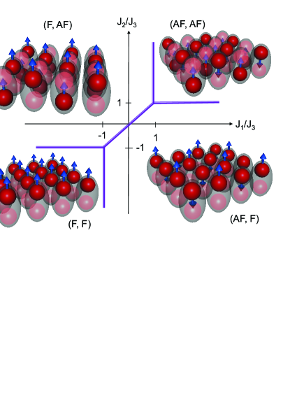
Figure 2: (Color online) The mean field phase diagram of symmetrical model (11) for $J_{3}>0$, see, e.g., Refs. Oleś et al. (2000); Ishihara et al. (1996) for $d$-electron compounds. Here “F” stands for ferromagnetic ordering, and “AF” is for antiferromagnetic ordering. The first and the second abbreviation in the designations of phases are for the spin and pseudospin subsystems, respectively. The ordering patterns of atoms on the optical lattice are shown in the insets. For ferromagnetic orbital arrangement atoms are localized in one particular type of sub-wells (for example in the upper sub-wells). For antiferromagnetic orbital arrangement atoms alternate between the lower and upper sub-wells. Red spheres show the lattice site with the maximum probability of occupation by atom, while transparent spheres show “nearly” empty sites. Arrows indicate spin directions.

Let us consider the most interesting case $\Delta^{x,z}\ll J_{1,2,3}$ and we can neglect the term $H_{\Delta}$ comparing with $H_{\operatorname{\mathrm{\scriptscriptstyle TUJ}}}$. Then the isolated minima of the double-well potential are the same. The spin-pseudospin interaction resulted from virtual hoppings between neighboring notches gives rise to the occupancy of that sub-well which is more preferable.

The properties of the Kugel-Khomskii symmetrical Hamiltonian (11) have been well investigated, see e.g., Refs. Kugel and Khomskii, 1973; Kugel’ and Khomskii, 1982. In Fig. 2 we present the result of the analysis of the model (11) in the mean-field approximation for $J_{3}>0$ [similarly would look like the figure for $J_{3}<0$ van den Brink et al. (1998)]. The figure shows possible phases of spin-pseudospin arrangements for various values of exchange parameters. For example, the case $J_{1}>J_{3}>J_{2}>0$ corresponds to the ground state of $H_{\rm sym}$ which is antiferromagnetic in the spin space and ferromagnetic in the pseudospin space, (AF-F) phase in Fig. 2. The effective orbital exchange can be estimated as $J_{\tau}^{\rm eff}=J_{2}+4J_{3}\langle{\mathbf{S}}_{i}\cdot{\mathbf{S}}_{j}\rangle$. Similarly the effective spin-exchange is approximately equal to $J_{s}^{\rm eff}=J_{1}+4J_{3}\langle{\bm{\tau}}_{i}\cdot{\bm{\tau}}_{j}\rangle$. When spins are antiferromagnetically ordered $J_{\tau}^{\rm eff}=J_{2}-J_{3}<0$ and one obtains “orbital ferromagnetism”. If we turn on the external effective magnetic field we can change the orbital ferromagnetism to orbital antiferromagnetism when the field is sufficiently strong that $\langle{\textbf{S}}_{i}\cdot{\textbf{S}}_{j}\rangle>J_{2}/4J_{3}$. Finite $\Delta^{x}$, $\Delta^{z}$ play the role of the built-in effective magnetic field in the pseudo-spin space. Large enough $\Delta^{z}$ would also drive the system into the ferromagnetic orbital state (in such a case one of the two minima of the double well is much lower than the other).

To illustrate the possible arrangement patterns of atoms in real space let us consider pseudospin (orbital) state in the mean field approximation . It can be presented as a product of one-site orbital states, $|\psi_{\rm mf}\rangle=\prod_{i}|\theta_{i}\varphi_{i}\rangle$. The orbital one-site state $|\theta_{i}\varphi_{i}\rangle$ can be chosen as

$$|\theta_{i}\varphi_{i}\rangle=\cos\frac{\theta_{i}}{2}|1\rangle+e^{i\varphi_{i}}\sin\frac{\theta_{i}}{2}|2\rangle.$$ (12)

The direction (in pseudospin space) of the averaged pseudospin $\langle{\bm{\tau}}_{i}\rangle$ is defined in terms of the polar and azimuth angles

$$\langle\theta_{i}\varphi_{i}|{\bm{\tau}}_{i}|\theta_{i}\varphi_{i}\rangle=\frac{1}{2}\left(\sin\theta_{i}\cos\varphi_{i},{\>}\sin\theta_{i}\sin\varphi_{i},{\>}\cos\theta_{i}\right).$$ (13)

The orbital state

$$|\pi-\theta_{i},{\;}\pi+\varphi_{i}\rangle=\sin\frac{\theta_{i}}{2}|1\rangle-e^{i\varphi_{i}}\cos\frac{\theta_{i}}{2}|2\rangle$$ (14)

is orthogonal to $|\theta_{i}{\,}\varphi_{i}\rangle$ and sets $\langle{\bm{\tau}}_{i}\rangle$ in the opposite direction. Ferromagnetic orbital arrangement corresponds to identical orbital states $|\theta_{i}{\,}\varphi_{i}\rangle=|\theta{\,}\varphi\rangle$ at different sites. Antiferromagnetic orbital state corresponds to $|\theta_{i}{\,}\varphi_{i}\rangle=|\theta{\,}\varphi\rangle$ at sublattice $i\in A$, and $|\theta_{j}{\,}\varphi_{j}\rangle=|\pi-\theta,{\,}\pi+\varphi\rangle$ at sublattice $i\in B$. The average pseudospin vectors alternate at the sublattices $A$ and $B$, $\langle{\bm{\tau}}_{i}\rangle=-\langle{\bm{\tau}}_{j}\rangle$.

The most simple illustration of the orbital arrangement of atoms can be given for the case of $\theta=0$, or $\theta=\pi$. Then atoms with probability equal to one occupy either well $\alpha=1$, or $\alpha=2$, respectively. The illustrative example of “phase diagrams” for this case is sketched in Fig. 2 where we adopted results of Refs. Feiner et al., 1997; van den Brink et al., 1998; Oleś et al., 2000; Ishihara et al., 1996 on the Kugel-Khomskii model to our problem of atom arrangements on the optical lattice (see also Supplementary Material Sup, ). The sketch shows the ordering patterns of atoms on the optical lattice of the type presented in Fig. 1b. For the ferromagnetic orbital arrangement atoms are localized in one of the sub-wells, for example in upper sub-wells. For the antiferromagnetic arrangement atoms alternates between $\alpha=1$ and $\alpha=2$ wells (upper and lower wells in figure). If we consider the antiferromagnetic orbital arrangement beyond the mean field approximation then atoms are spread between two sub-wells with some probability due to quantum fluctuation. Red spheres in Fig. 2 show lattice sites with the maximum probability of occupation by atom, while white spheres show “nearly” empty sites. Arrows indicate spin directions. The phase boundaries in Fig. 2 actually do not exactly match coordinate axes in $(J_{1},J_{2})$ space: the absolute value and sign of $J_{3}$ specify the position of the phase boundaries Feiner et al. (1997); van den Brink et al. (1998); Oleś et al. (2000); Ishihara et al. (1996), as is illustrated.

III.2 Complex hopping amplitudes

One of the unique properties of optical lattices is the possibility to tune the complex tunnel amplitudes by manipulating the laser field Struck et al. (2012). It includes also the possibility to manipulate the Hamiltonian by changing the phases of the hopping amplitudes $t_{ij}$ and leaving their absolute values fixed (i.e. no geometric distortion of the optical lattice).

Toy model

To illustrate the importance of the complex phases of the hopping amplitudes $t_{ij}$ we consider the following toy-model. We suppose that $\operatorname{\mathit{J}_{\mathrm{\scriptscriptstyle H}}}=0$ and we account for those hoppings which go through different orbitals (wells):

$$t^{11}=0,\quad t^{22}=0,\quad t^{12}=t^{\prime},\quad t^{21}=t^{\prime}e^{i\chi}.$$ (15)

The constant phase $\chi$ accounts for phase difference in the non-diagonal hopping amplitudes. Then the effective Hamiltonian (9) can be written as (see Appendix A)

$$H_{\chi}=J{\,}\sum\limits_{\langle ij\rangle}\Bigl{(}\frac{1}{2}+2{\,}{\bf S}_{i}\cdot{\bf S}_{j}\Bigr{)}\Bigl{(}\frac{1}{2}+2\cos\chi{\,}(\tau^{x}_{i}\tau^{x}_{j}-\tau^{y}_{i}\tau^{y}_{j})+\\ +2\sin\chi{\,}(\tau^{x}_{i}\tau^{y}_{j}+\tau^{y}_{i}\tau^{x}_{j})-2\tau^{z}_{i}\tau^{z}_{j}\Bigr{)}.$$ (16)

The appearance of the phase-dependent ground state can be illustrated as the following. For the ferromagnetic spin background the mean field energy $E_{\rm mf}=\langle\psi_{\rm mf}|H_{\chi}|\psi_{\rm mf}\rangle$ of pseudospin sub-system is

$$E_{\rm mf}=\frac{J}{2}\sum\limits_{\langle i,j\rangle}\Bigl{[}1+\cos(\chi-(\varphi_{i}+\varphi_{j}))\sin\theta_{i}\sin\theta_{j}-\\ -\cos\theta_{i}\cos\theta_{j}\Bigr{]},$$ (17)

where we used $1/2+2{\bf S}_{i}{\bf S}_{j}=1$. Consider now the energy of the antiferromagnetic orbital state. For such a state the mean field energy per site is

$$E_{\rm mf}=\frac{3}{2}J\Bigl{[}1-\cos(\chi-2\varphi)\sin^{2}\theta+\cos^{2}\theta\Bigr{]}.$$ (18)

The minimization of the energy $E_{mf}$ relative to $\theta$ and $\varphi$ gives the twofold degenerate ground state $E_{gs}=0$ with $\theta=\pi/2$ and $\varphi=\chi/2,\chi/2+\pi$, The resulting direction of the pseudospin $\langle{\bm{\tau}}\rangle$ depends on the phase $\chi$. In real space this state describes the situation when the atoms with equal probability are spread over the first and second wells in the notch but the phase relation between pseudospin states $|1\rangle$ and $|2\rangle$ are tuned by the applied phase $\chi$. The change of $\chi$ induces the corresponding variation of the phase $\varphi$, which is equivalent to rotation of the pseudospin vector $\langle{\bm{\tau}}\rangle$ in the pseudospin space.

Conclusions

Optical lattices are quantum simulators of many-particle systems. We have shown that there is a mapping between fermion quantum ordering in the optical superlattices and the spin-orbital physics developed for degenerate $d$-electron compounds. The effective spin-pseudospin model has been derived. This model is the generalization of the Kugel-Khomskii Hamiltonian for complex hopping amplitudes. We have shown how different ground states of this Hamiltonian correspond to particular nontrivial fermion arrangements on the lattice.

Appendix A Perturbative expansion in hopping amplitudes

In the subspace of functions $|\Phi^{0}\rangle$ with occupancy equal to one at each site the hopping term $\operatorname{\mathit{H}_{\mathrm{\scriptscriptstyle T}}}$ creates intermediate states with double occupancy. There are six different intermediate states with double occupancy at a given site $i$, which differ in the well $\alpha$ and spin $\sigma$ indices

$$|\psi_{1}\rangle=\begin{pmatrix}\frac{\quad}{\quad}{\!}{\!}\frac{\quad}{\quad}{\!}{\!}\frac{\quad}{\quad}\\ \frac{\quad}{\quad}{\!}{\!}{\!}{\!}\uparrow{\!}{\!}{\!}{\!}\frac{\;\;\>}{\;\;\;}{\!}{\!}{\!}{\!}\downarrow{\!}{\!}{\!}{\!}\frac{\quad}{\quad}{\!}{\!}\frac{\;\>}{\;\;}\end{pmatrix},\qquad|\psi_{2}\rangle=\begin{pmatrix}\frac{\quad}{\quad}{\!}{\!}{\!}{\!}\uparrow{\!}{\!}{\!}{\!}\frac{\;\;\>}{\;\;\;}{\!}{\!}{\!}{\!}\downarrow{\!}{\!}{\!}{\!}\frac{\quad}{\quad}{\!}{\!}\frac{\;\>}{\;\;}\\ \frac{\quad}{\quad}{\!}{\!}\frac{\quad}{\quad}{\!}{\!}\frac{\quad}{\quad}\end{pmatrix}$$ (19)

$$|\psi_{3}\rangle=\begin{pmatrix}\frac{\quad}{\quad}{\!}{\!}{\!}{\!}\frac{\;\;\;}{\;\;\;}{\!}{\!}\uparrow{\!}{\!}{\!}{\!}{\!}{\!}{\!}{\!}\frac{\qquad}{\qquad}\\ \frac{\quad}{\quad}{\!}{\!}{\!}{\!}\uparrow{\!}{\!}{\!}{\!}{\!}{\!}{\!}{\!}\frac{\qquad}{\qquad}{\!}{\!}\frac{\;\;}{\;\;}\end{pmatrix},\qquad|\psi_{4}\rangle=\begin{pmatrix}\frac{\quad}{\quad}{\!}{\!}{\!}{\!}\frac{\;\;\;}{\;\;\;}{\!}{\!}\downarrow{\!}{\!}{\!}{\!}{\!}{\!}{\!}{\!}\frac{\qquad}{\qquad}\\ \frac{\quad}{\quad}{\!}{\!}{\!}{\!}\downarrow{\!}{\!}{\!}{\!}{\!}{\!}{\!}{\!}\frac{\qquad}{\qquad}{\!}{\!}\frac{\;\;}{\;\;}\end{pmatrix}$$ (20)

$$|\psi_{5}\rangle=\begin{pmatrix}\frac{\quad}{\quad}{\!}{\!}{\!}{\!}\frac{\;\;\;}{\;\;\;}{\!}{\!}\downarrow{\!}{\!}{\!}{\!}{\!}{\!}{\!}{\!}\frac{\qquad}{\qquad}\\ \frac{\quad}{\quad}{\!}{\!}{\!}{\!}\uparrow{\!}{\!}{\!}{\!}{\!}{\!}{\!}{\!}\frac{\qquad}{\qquad}{\!}{\!}\frac{\;\;}{\;\;}\end{pmatrix},\qquad|\psi_{6}\rangle=\begin{pmatrix}\frac{\quad}{\quad}{\!}{\!}{\!}{\!}\frac{\;\;\;}{\;\;\;}{\!}{\!}\uparrow{\!}{\!}{\!}{\!}{\!}{\!}{\!}{\!}\frac{\qquad}{\qquad}\\ \frac{\quad}{\quad}{\!}{\!}{\!}{\!}\downarrow{\!}{\!}{\!}{\!}{\!}{\!}{\!}{\!}\frac{\qquad}{\qquad}{\!}{\!}\frac{\;\;}{\;\;}\end{pmatrix}$$ (21)

Here the lower (upper) level is for the pseudospin state $\alpha=1(2)$. All of them are eigenstates of the $\operatorname{\mathit{H}_{\mathrm{\scriptscriptstyle U}}}$ with the same energy $U$ and the first four are also eigenstates of $\operatorname{\mathit{H}_{\mathrm{\scriptscriptstyle J}}}$. Although the term $\operatorname{\mathit{H}_{\mathrm{\scriptscriptstyle J}}}$ mixes the states $|\psi_{5}\rangle$ and $|\psi_{6}\rangle$ it mixes them into eigenstate of $\operatorname{\mathit{H}_{\mathrm{\scriptscriptstyle U}}}$.

In the second order perturbation theory in hopping term $\operatorname{\mathit{H}_{\mathrm{\scriptscriptstyle T}}}$ the effective Hamiltonian has the form Auerbach (1994)

$$H_{\operatorname{\mathrm{\scriptscriptstyle TUJ}}}=-\operatorname{\mathit{H}_{\mathrm{\scriptscriptstyle T}}}\frac{1}{\operatorname{\mathit{H}_{\mathrm{\scriptscriptstyle U}}}+\operatorname{\mathit{H}_{\mathrm{\scriptscriptstyle J}}}}\operatorname{\mathit{H}_{\mathrm{\scriptscriptstyle T}}}.$$ (22)

Assuming that $\operatorname{\mathit{J}_{\mathrm{\scriptscriptstyle H}}}\ll U$ the above expression in first order of $\operatorname{\mathit{J}_{\mathrm{\scriptscriptstyle H}}}/U$ can be simplified as

$$H_{\operatorname{\mathrm{\scriptscriptstyle TUJ}}}=-\operatorname{\mathit{H}_{\mathrm{\scriptscriptstyle T}}}\left[\frac{1}{\operatorname{\mathit{H}_{\mathrm{\scriptscriptstyle U}}}}-\frac{1}{\operatorname{\mathit{H}_{\mathrm{\scriptscriptstyle U}}}}\operatorname{\mathit{H}_{\mathrm{\scriptscriptstyle J}}}.\frac{1}{\operatorname{\mathit{H}_{\mathrm{\scriptscriptstyle U}}}}\right]\operatorname{\mathit{H}_{\mathrm{\scriptscriptstyle T}}}$$ (23)

As we mentioned above all the intermediate states (19), (20) and (21) after mixing them by $\operatorname{\mathit{H}_{\mathrm{\scriptscriptstyle J}}}$ remain eigenstates of $\operatorname{\mathit{H}_{\mathrm{\scriptscriptstyle U}}}$. It enables to reduce the above expression for $H_{\operatorname{\mathrm{\scriptscriptstyle TUJ}}}$ to the following form

$$H_{\operatorname{\mathrm{\scriptscriptstyle TUJ}}}=-\frac{1}{U}\left(\operatorname{\mathit{H}^{2}_{\mathrm{\scriptscriptstyle T}}}-\frac{1}{U}\operatorname{\mathit{H}_{\mathrm{\scriptscriptstyle T}}}\operatorname{\mathit{H}_{\mathrm{\scriptscriptstyle J}}}\operatorname{\mathit{H}_{\mathrm{\scriptscriptstyle T}}}\right).$$ (24)

Presentation of fermi-operators through the spin and pseudospin operators which is originally due to Kugel and Khomskii Kugel and Khomskii (1973) can be given as

$$c^{\dagger}_{i\alpha\gamma}c_{i\beta\gamma^{\prime}}=\left(\frac{1}{2}\delta_{\alpha\beta}+\tau_{i}^{a}\sigma^{a}_{\beta\alpha}\right)\left(\frac{1}{2}\delta_{\gamma\gamma^{\prime}}+S_{i}^{b}\sigma^{b}_{\gamma^{\prime}\gamma}\right).$$ (25)

In the subspace of functions $|\Phi^{0}\rangle$ the first and the second term of the $\operatorname{\mathit{H}^{2}_{\mathrm{\scriptscriptstyle T}}}$ is reduced to

$$\operatorname{\mathit{H}^{2}_{\mathrm{\scriptscriptstyle T}}}=\sum\limits_{\langle ij\rangle}\biggl{\{}{\rm Sp}(t^{\dagger}t)+{\rm Sp}(t^{\dagger}\sigma^{a}t){\,}\tau^{a}_{i}+{\rm Sp}(t\sigma^{a}t^{\dagger}){\,}\tau^{a}_{j}-\\ \left(\frac{1}{2}+2{\,}{\bf S}_{i}\cdot{\bf S}_{j}\right)\Bigl{[}\frac{1}{2}{\rm Sp}(t^{\dagger}t)+{\rm Sp}(t^{\dagger}\sigma^{a}t){\,}\tau^{a}_{i}+{\rm Sp}(t\sigma^{a}t^{\dagger}){\,}\tau^{a}_{j}+2{\,}{\rm Sp}(t^{\dagger}\sigma^{a}t\sigma^{b}t){\,}\tau^{a}_{i}\tau^{b}_{j}\Bigr{]}\biggr{\}},$$ (26)

$$\frac{1}{U}\operatorname{\mathit{H}_{\mathrm{\scriptscriptstyle T}}}\operatorname{\mathit{H}_{\mathrm{\scriptscriptstyle J}}}\operatorname{\mathit{H}_{\mathrm{\scriptscriptstyle T}}}=\left(\frac{-\operatorname{\mathit{J}_{\mathrm{\scriptscriptstyle H}}}}{U}\right)\sum\limits_{\langle ij\rangle}\biggl{\{}-\frac{1}{2}{\,}{\rm Sp}(t^{\dagger}\sigma^{a^{\prime}}t)\tau^{a^{\prime}}_{i}-\frac{1}{2}{\,}{\rm Sp}(t\sigma^{a^{\prime}}t^{\dagger})\tau^{a^{\prime}}_{j}-{\rm Sp}(t^{\dagger}\sigma^{a^{\prime}}\sigma^{b}t)\tau^{a^{\prime}}_{i}\tau^{b}_{j}-{\rm Sp}(t^{\dagger}\sigma^{b}t\sigma^{a^{\prime}})\tau^{b}_{i}\tau^{a^{\prime}}_{j}+\\ \left(\frac{1}{2}+2{\bf S}_{i}\cdot{\bf S}_{j}\right)\Bigl{[}\frac{1}{2}{\,}{\rm Sp}(t^{\dagger}t)+\frac{1}{2}{\,}{\rm Sp}(t^{\dagger}\sigma^{a^{\prime}}t)\tau^{a^{\prime}}_{i}+\frac{1}{2}{\,}{\rm Sp}(t\sigma^{a^{\prime}}t^{\dagger})\tau^{a^{\prime}}_{j}-{\rm Sp}(t^{\dagger}\sigma^{z}t\sigma^{a})\tau^{z}_{i}\tau^{a}_{j}-{\rm Sp}(t^{\dagger}\sigma^{a}t\sigma^{z})\tau^{a}_{i}\tau^{z}_{j}\Bigr{]}\biggr{\}}$$ (27)

The summation over repeated indices $a,b=1,2,3$ is implied, indices with prime mean that the summation does not include the third component, i.e. $a^{\prime},b^{\prime}=1,2$. In terms proportional to $\tau^{a}_{j}$ we used the property of the Hermitian conjugate hopping matrix $t^{\alpha\beta}_{ji}=(t^{\dagger})^{\alpha\beta}_{ij}$.

In what follows we omit the constant term ${\rm Sp}(t^{\dagger}t)$ in $\operatorname{\mathit{H}^{2}_{\mathrm{\scriptscriptstyle T}}}$. Gathering both terms together we obtain after regrouping the following effective Hamiltonian

$$H_{\operatorname{\mathrm{\scriptscriptstyle TUJ}}}=\sum\limits_{\langle ij\rangle}{\,}\biggl{[}\frac{1}{4}A_{ij}+A_{ij}{\,}{\bf S}_{i}\cdot{\bf S}_{j}+B^{ab}_{ij}{\,}\tau^{a}_{i}\tau^{b}_{j}-\frac{1}{2}(K_{ij}^{a}{\,}\tau^{a}_{i}+K_{ji}^{a}{\,}\tau^{a}_{j})+4{\>}{\bf S}_{i}\cdot{\bf S}_{j}\Bigl{\{}D^{ab}_{ij}{\,}\tau^{a}_{i}\tau^{b}_{j}+\frac{1}{2}(K_{ij}^{a}{\,}\tau^{a}_{i}+K_{ji}^{a}{\,}\tau^{a}_{j})\Bigr{\}}\biggr{]},$$ (28)

where

$$A_{ij}=\frac{1}{U}{\,}{\rm Sp}(t\,t^{\dagger})\left(1-\frac{\operatorname{\mathit{J}_{\mathrm{\scriptscriptstyle H}}}}{U}\right).$$ (29)

$$B^{ab}_{ij}=\frac{1}{U}{\,}{\rm Sp}(t^{\dagger}\sigma^{a}t\sigma^{b})\left\{\begin{aligned} 1&+\frac{2\operatorname{\mathit{J}_{\mathrm{\scriptscriptstyle H}}}}{U},&a,b=1,2\\ 1&+\frac{3\operatorname{\mathit{J}_{\mathrm{\scriptscriptstyle H}}}}{2U},&{a=1,2,b=3\atop a=3,b=1,2}\\ 1&+\frac{\operatorname{\mathit{J}_{\mathrm{\scriptscriptstyle H}}}}{U},&a,b=3\\ \end{aligned}\right.$$ (30)

$$D^{ab}_{ij}=\frac{1}{U}{\,}{\rm Sp}(t^{\dagger}\sigma^{a}t\sigma^{b})\left\{\begin{aligned} 1&,&a,b=1,2\\ 1&+\frac{\operatorname{\mathit{J}_{\mathrm{\scriptscriptstyle H}}}}{2U},&{a=1,2,b=3\atop a=3,b=1,2}\\ 1&+\frac{\operatorname{\mathit{J}_{\mathrm{\scriptscriptstyle H}}}}{U},&a,b=3\\ \end{aligned}\right.$$ (31)

$$K^{a}_{ij}=\frac{1}{U}{\,}{\rm Sp}(t^{\dagger}\sigma^{a}t)\left\{\begin{aligned} 1&-\frac{\operatorname{\mathit{J}_{\mathrm{\scriptscriptstyle H}}}}{2U},&a&=1,2\\ 1&,&a&=3\\ \end{aligned}\right.$$ (32)

Vectors $K^{a}_{ji}$, which enter in Eq. 28, are proportional to ${\rm Sp}(t^{\dagger}_{ji}\sigma^{a}t_{ji})$. They can be given in terms of $t_{ij}$ using the equality ${\rm Sp}(t^{\dagger}_{ji}\sigma^{a}t_{ji})={\rm Sp}(t_{ij}\sigma^{a}t^{\dagger}_{ij})$. Note also that for zero Hund’s coupling, $J_{H}=0$, the second rank tensors are the similar, $B^{ab}_{ij}=D^{ab}_{ij}$.

The presentation in the form (28) can be viewed as a generalization of the corresponding Kugel-Khomskii Kugel and Khomskii (1973) Hamiltonian for complex hopping amplitudes. Below we write down the explicit form of all the traces that contribute to the coefficients of the Hamiltonian:

$${\rm Sp}(t^{\dagger}t) = |t^{11}|^{2}+|t^{22}|^{2}+|t^{12}|^{2}+|t^{21}|^{2}$$

$${\rm Sp}(t^{\dagger}\sigma^{z}t) = |t^{11}|^{2}-|t^{22}|^{2}+|t^{12}|^{2}-|t^{21}|^{2}$$

$${\rm Sp}(t\sigma^{z}t^{\dagger}) = |t^{11}|^{2}-|t^{22}|^{2}+|t^{21}|^{2}-|t^{12}|^{2}$$

$${\rm Sp}(t^{\dagger}\sigma^{z}t\sigma^{z}) = |t^{11}|^{2}+|t^{22}|^{2}-|t^{12}|^{2}-|t^{21}|^{2}$$

$${\rm Sp}(t^{\dagger}\sigma^{x}t) = 2\operatorname{Re}[t^{11}(t^{21})^{*}+t^{22}(t^{12})^{*}]$$

$${\rm Sp}(t\sigma^{x}t^{\dagger}) = 2\operatorname{Re}[t^{11}(t^{12})^{*}+t^{22}(t^{21})^{*}]$$

$${\rm Sp}(t^{\dagger}\sigma^{y}t) = 2\operatorname{Im}[-t^{11}(t^{21})^{*}+t^{22}(t^{12})^{*}]$$

$${\rm Sp}(t\sigma^{y}t^{\dagger}) = 2\operatorname{Im}[t^{11}(t^{12})^{*}-t^{22}(t^{21})^{*}]$$

$${\rm Sp}(t^{\dagger}\sigma^{x}t\sigma^{x}) = 2\operatorname{Re}[t^{11}(t^{22})^{*}+t^{12}(t^{21})^{*}]$$

$${\rm Sp}(t^{\dagger}\sigma^{y}t\sigma^{y}) = 2\operatorname{Re}[t^{11}(t^{22})^{*}-t^{12}(t^{21})^{*}]$$

$${\rm Sp}(t^{\dagger}\sigma^{x}t\sigma^{y}) = 2\operatorname{Im}[t^{11}(t^{22})^{*}-t^{12}(t^{21})^{*}]$$

$${\rm Sp}(t^{\dagger}\sigma^{y}t\sigma^{x}) = 2\operatorname{Im}[-t^{11}(t^{22})^{*}-t^{12}(t^{21})^{*}]$$

$${\rm Sp}(t^{\dagger}\sigma^{x}t\sigma^{z}) = 2\operatorname{Re}[t^{11}(t^{21})^{*}-t^{22}(t^{12})^{*}]$$

$${\rm Sp}(t^{\dagger}\sigma^{z}t\sigma^{x}) = 2\operatorname{Re}[t^{11}(t^{12})^{*}-t^{22}(t^{21})^{*}]$$

$${\rm Sp}(t^{\dagger}\sigma^{z}t\sigma^{y}) = 2\operatorname{Im}[t^{11}(t^{12})^{*}+t^{22}(t^{21})^{*}]$$

$${\rm Sp}(t^{\dagger}\sigma^{y}t\sigma^{z}) = 2\operatorname{Im}[-t^{11}(t^{21})^{*}-t^{22}(t^{12})^{*}]$$

For specific choices of $t^{\alpha\beta}$, in particular for those considered in the paper, $K^{a}_{ji}=K^{a}_{ij}$, and the general form (28) is reduced to the Eq. 9 of the main text.

For the case of real site-independent hopping amplitudes $t^{11}=t_{1}$, $t^{22}=t_{2}$, $t^{12}=t^{21}=t_{12}$ the Hamiltonian (28) is reduced to the original Kugel-Khomskii Hamiltonian

$$H_{\operatorname{\mathrm{\scriptscriptstyle KK}}}=\frac{1}{U}\sum\limits_{\langle ij\rangle}\biggl{[}-(t_{1}^{2}-t_{2}^{2})(\tau^{z}_{i}+\tau^{z}_{j})-\left(1-\frac{J_{H}}{2U}\right)2t_{12}(t_{1}+t_{2})(\tau^{x}_{i}+\tau^{x}_{j})+\\ \frac{J_{H}}{U}{\,}4(t_{1}t_{2}+t_{12}^{2})\tau^{x}_{i}\tau^{x}_{j}+\frac{J_{H}}{U}{\,}4(t_{1}t_{2}-t_{12}^{2})\tau^{y}_{i}\tau^{y}_{j}+\frac{J_{H}}{U}{\,}2t_{12}(t_{1}-t_{2})(\tau^{z}_{i}\tau^{x}_{j}+\tau^{x}_{i}\tau^{z}_{j})+\\ \Bigl{(}\frac{1}{2}+2{\bf S}_{i}\cdot{\bf S}_{j}\Bigr{)}\biggl{\{}\left(1-\frac{J_{H}}{U}\right)\frac{1}{2}(t_{1}^{2}+t_{2}^{2}+2t_{12}^{2})+(t_{1}^{2}-t_{2}^{2})(\tau^{z}_{i}+\tau^{z}_{j})+\left(1-\frac{J_{H}}{2U}\right)2t_{12}(t_{1}+t_{2})(\tau^{x}_{i}+\tau^{x}_{j})+\\ 4(t_{1}t_{2}+t_{12}^{2})\tau^{x}_{i}\tau^{x}_{j}+4(t_{1}t_{2}-t_{12}^{2})\tau^{y}_{i}\tau^{y}_{j}+\left(1+\frac{J_{H}}{U}\right)2(t_{1}^{2}+t_{2}^{2}-2t_{12}^{2})\tau^{z}_{i}\tau^{z}_{j}+\left(1+\frac{J_{H}}{2U}\right)4t_{12}(t_{1}-t_{2})(\tau^{z}_{i}\tau^{x}_{j}+\tau^{x}_{i}\tau^{z}_{j})\biggr{\}}\biggr{]}$$ (33)

For diagonal hopping matrix $t_{12}=0$, and $t_{1}=t_{2}=t$ the Hamiltonian (33) is simplified to

$$H_{\operatorname{\mathrm{\scriptscriptstyle KK}}}=\frac{1}{4}J_{1}+J_{1}{\bf S}_{i}\cdot{\bf S}_{j}+J_{2}{\bm{\tau}}_{i}\cdot{\bm{\tau}}_{j}+4J_{3}({\bf S}_{i}\cdot{\bf S}_{j}){\,}({\bm{\tau}}_{i}\cdot{\bm{\tau}}_{j})-J_{3}\Bigl{(}1-4{\,}{\bf S}_{i}\cdot{\bf S}_{j}\Bigr{)}\frac{J_{H}}{U}{\,}\tau^{z}_{i}\tau^{z}_{j}$$ (34)

where

$$J_{1}=\frac{2t^{2}}{U}\Bigl{(}1-\frac{J_{H}}{U}\Bigr{)},$$ (35)

$$J_{2}=\frac{2t^{2}}{U}\Bigl{(}1+2\frac{J_{H}}{U}\Bigr{)},$$ (36)

$$J_{3}=\frac{2t^{2}}{U}$$ (37)

The Hamiltonian serves as a starting form for the symmetrical Hamiltonian (11) with independent $J_{1}$, $J_{2}$ and $J_{3}$, if one neglects anisotropy term ($\propto J_{H}/U{\,}\tau^{z}_{i}\tau^{z}_{j}$) in pseudospin space.

Toy model

To illustrate the meaning of complex phases we have considered hereinabove the case when hopping process can be described by the following toy-model

$$t^{11}=0,\quad t^{22}=0,\quad t^{12}=t^{\prime},\quad t^{21}=t^{\prime}e^{i\chi}.$$ (38)

For such amplitudes the only nonzero traces are

$${\rm Sp}(tt^{\dagger})=2|t^{\prime}|^{2},\quad{\rm Sp}(\sigma^{z}t\sigma^{z}t^{\dagger})=-2|t^{\prime}|^{2}$$ (39)

$${\rm Sp}(\sigma^{x}t\sigma^{x}t^{\dagger})=-{\rm Sp}(\sigma^{y}t\sigma^{y}t^{\dagger})=2|t^{\prime}|^{2}\cos\chi$$ (40)

$${\rm Sp}(\sigma^{x}t\sigma^{y}t^{\dagger})={\rm Sp}(\sigma^{y}t\sigma^{x}t^{\dagger})=2|t^{\prime}|^{2}\sin\chi$$ (41)

The Hamiltonian $H_{\operatorname{\mathrm{\scriptscriptstyle TUJ}}}$ can be rewritten as

$$H_{\chi}=J{\,}\sum\limits_{\langle ij\rangle}\Bigl{(}\frac{1}{2}+2{\,}{\bf S}_{i}\cdot{\bf S}_{j}\Bigr{)}\Bigl{(}\frac{1}{2}+2B^{ab}{\,}\tau^{a}_{i}\tau^{b}_{j}\Bigr{)}$$ (42)

where effective exchange is $J=2|t^{\prime}|^{2}/U$ and $B^{12}=B^{21}=\sin\chi$, $B^{11}=-B^{22}=\cos\chi$, $B^{33}=-1$. The Eq. 42 can be rewritten in the form (16).

References

• Greiner et al. (2002) M. Greiner, O. Mandel, T. Esslinger, T. W. Hänsch,  and I. Bloch, Nature 415, 39 (2002).
• Köhl et al. (2005) M. Köhl, H. Moritz, T. Stöferle, K. Günter,  and T. Esslinger, Phys. Rev. Lett. 94, 080403 (2005).
• Kawaguchi and Ueda (2012) Y. Kawaguchi and M. Ueda, Phys. Rep. 253, 253 (2012).
• Hauke et al. (2012) P. Hauke, F. M. Cucchietti, L. Tagliacozzo, I. Deutsch,  and M. Lewenstein, Rep. Prog. Phys. 75, 082401 (2012).
• Meacher (1998) D. R. Meacher, Contemp. Phys. 39, 329 (1998).
• Jaksch et al. (1998) D. Jaksch, C. Bruder, J. I. Cirac, C. W. Gardiner,  and P. Zoller, Phys. Rev. Lett. 81, 3108 (1998).
• Grimm et al. (2000) R. Grimm, M. Weidemuller,  and Y. B. Ovchinnikov (Academic Press, 2000) pp. 95 – 170.
• Corboz et al. (2012) P. Corboz, M. Lajkó, A. M. Läuchli, K. Penc,  and F. Mila, Phys. Rev. X 2, 041013 (2012).
• Bloch et al. (2008) I. Bloch, J. Dalibard,  and W. Zwerger, Rev. Mod. Phys. 80, 885 (2008).
• Quéméner and Julienne (2012) G. Quéméner and P. S. Julienne, Chem. Rev. 112, 4949 (2012).
• Lewenstein et al. (2007) M. Lewenstein, A. Sanpera, V. Ahufinger, B. Damski, A. Sen(De),  and U. Sen, Adv. Phys. 56, 243 (2007).
• Wagner et al. (2011) A. Wagner, C. Bruder,  and E. Demler, Phys. Rev. A 84, 063636 (2011).
• Jördens et al. (2008) R. Jördens, N. Strohmaier, K. Günter, H. Moritz,  and T. Esslinger, Nature 455, 204 (2008).
• Anderlini et al. (2007a) M. Anderlini, P. J. Lee, B. L. Brown, J. Sebby-Strabley, W. D. Phillips,  and J. Porto, Nature 448, 452 (2007a).
• Fölling et al. (2007) S. Fölling, S. Trotzky, P. Cheinet, M. Feld, R. Saers, A. Widera, T. Müller,  and I. Bloch, Nature 448, 1029 (2007).
• Anderlini et al. (2007b) M. Anderlini, P. J. Lee, B. L. Brown, J. Sebby-Strabley, W. D. Phillips,  and J. Porto, Nature 448, 452 (2007b).
• Trotzky et al. (2008) S. Trotzky, P. Cheinet, S. Fölling, M. Feld, U. Schnorrberger, A. Rey, A. Polkovnikov, E. Demler, M. Lukin,  and I. Bloch, Science 319, 295 (2008).
• Wagner et al. (2012) A. Wagner, A. Nunnenkamp,  and C. Bruder, Phys. Rev. A 86, 023624 (2012).
• Kugel and Khomskii (1973) K. Kugel and D. Khomskii, Zh. Eksp. Teor. Fiz 64, 1429 (1973).
• Kugel’ and Khomskii (1982) K. I. Kugel’ and D. I. Khomskii, Uspekhi Fizicheskikh Nauk 136, 621 (1982).
• Abrikosov (1965) A. Abrikosov, Physics 2, 5 (1965).
• Yamashita et al. (1998) Y. Yamashita, N. Shibata,  and K. Ueda, Phys. Rev. B 58, 9114 (1998).
• Auerbach (1994) A. Auerbach, Interacting electrons and quantum magnetism (Springer Verlag, 1994).
• Feiner et al. (1997) L. F. Feiner, A. M. Oleś,  and J. Zaanen, Phys. Rev. Lett. 78, 2799 (1997).
• Ishihara et al. (1997) S. Ishihara, J. Inoue,  and S. Maekawa, Phys. Rev. B 55, 8280 (1997).
• Brzezicki et al. (2013) W. Brzezicki, J. Dziarmaga,  and A. M. Oleś, Phys. Rev. B 87, 064407 (2013).
• Oleś et al. (2000) A. M. Oleś, L. Felix Feiner,  and J. Zaanen, Phys. Rev. B 61, 6257 (2000).
• Ishihara et al. (1996) S. Ishihara, J. Inoue,  and S. Maekawa, Physica C 263, 130 (1996).
• van den Brink et al. (1998) J. van den Brink, W. Stekelenburg, D. I. Khomskii, G. A. Sawatzky,  and K. I. Kugel, Phys. Rev. B 58, 10276 (1998).
• (30) Supplemental Material .
• Struck et al. (2012) J. Struck, C. Ölschläger, M. Weinberg, P. Hauke, J. Simonet, A. Eckardt, M. Lewenstein, K. Sengstock,  and P. Windpassinger, Phys. Rev. Lett. 108, 225304 (2012).