Subarcsecond Imaging of the NGC 6334 I(N) Protocluster:
Two Dozen Compact Sources and a Massive Disk Candidate

Abstract

Using the SMA and VLA, we have imaged the massive protocluster NGC 6334 I(N) at high angular resolution ($0.5^{\prime\prime}\sim 650$ AU) from 6 cm to 0.87 mm, detecting 18 new compact continuum sources. Three of the new sources are coincident with previously-identified H₂O masers. Together with the previously-known sources, these data bring the number of likely protocluster members to 25 for a protostellar density of $\sim 700$ pc^-3. Our preliminary measurement of the $Q$-parameter of the minimum spanning tree is 0.82 – close to the value for a uniform volume distribution. All of the (nine) sources with detections at multiple frequencies have SEDs consistent with dust emission, and two (SMA 1b and SMA 4) also have long wavelength emission consistent with a central hypercompact HII region. Thermal spectral line emission, including CH₃CN, is detected in six sources: LTE model fitting of CH₃CN ($J$=12–11) yields temperatures of 72–373 K, confirming the presence of multiple hot cores. The fitted LSR velocities range from $-3.3$ to $-7.0$ km s^-1, with an unbiased mean square deviation of 2.05 km s^-1, implying a protocluster dynamical mass of 410$\pm$260 $M_{\odot}$. From analysis of a wide range of hot core molecules, the kinematics of SMA 1b are consistent with a rotating, infalling Keplerian disk of diameter 800 AU and enclosed mass of 10-30 $M_{\odot}$ that is perpendicular (within $1\arcdeg$) to the large-scale bipolar outflow axis. A companion to SMA 1b at a projected separation of $0.45\arcsec\/$ (590 AU; SMA 1d), which shows no evidence of spectral line emission, is also confirmed. Finally, we detect one 218.4400 GHz and several 229.7588 GHz Class-I CH₃OH masers.

1 Introduction

Massive star formation is a phenomenon of fundamental importance in astrophysics yet a detailed understanding of it has been elusive (Zinnecker & Yorke, 2007). The present state of theory and numerical simulation research fall into two major categories of processes: “core accretion” and “competitive accretion”, as recently reviewed by Tan et al. (2014). In the core accretion scenario, massive stars (like low-mass stars) are formed via the collapse of self-gravitating, centrally condensed cores. These cores are discrete structures within the larger-scale molecular cloud, and each core constitutes the mass reservoir for a single star or small multiple system. As a result, core mass maps directly to stellar mass, and the core mass function (CMF) maps to the stellar initial mass function (IMF) (e.g. Myers et al., 2013; Krumholz et al., 2009; McKee & Tan, 2003, and references therein). In contrast, competitive accretion models are intrinsically models of star cluster formation. Fragmentation in a cluster-scale gas clump produces many low-mass protostars, which then accrete (competitively) from the large-scale gas reservoir. In this picture, massive stars must form in a cluster environment, and massive stars and their surrounding clusters must form simultaneously (e.g. Bonnell & Smith, 2011; Smith et al., 2009, and references therein).

There are several significant observational constraints that these theories must face. First, there is mass segregation – the fact that the most massive members of young clusters are concentrated in the center (e.g. Kirk & Myers, 2011). It remains unclear whether this property is primordial or a result of dynamical evolution. $N$-body simulations of star clusters have shown that it is common to form compact groupings of massive stars (i.e. Trapezium-like systems) near the center of the cluster in as little as one free-fall time, particularly when there is initial substructure (Allison & Goodwin, 2011). Observational studies of young clusters caught early in the act of forming are critical to address the origin of mass segregation. Second, there is the correlation between the mass of the most massive star and the number of cluster members (Hillenbrand, 1995; Testi et al., 1999). An ensuing question is whether the high-mass and low-mass members of clusters form at the same time. Perhaps the only way to answer this question is to search for actively forming low-mass protostars amidst their high-mass counterparts. Toward this end, the past decade of advances in (sub)millimeter interferometry has enabled the identification of proto-Trapezium-like systems, termed “protoclusters” (e.g. Hunter et al., 2006; Beuther et al., 2007a; Rodón et al., 2008), in which four or more compact millimeter continuum sources exist within a projected diameter of 10000 AU. In many cases, the protocluster members present a striking diversity in star formation indicators – including the presence or absence of H₂O masers, hot core line emission, and free-free emission – providing strong evidence that closely neighboring objects can exist in different evolutionary stages of formation (Zhang et al., 2007; Cyganowski et al., 2007; Brogan et al., 2008, 2011; Zinchenko et al., 2012). At last count of the literature, half of these massive cores studied at $\lesssim 1000$ AU resolution were resolved into four or more millimeter sources (Palau et al., 2013). These results emphasize the possibility of interaction between massive protostars, as well as their probable impact on low-mass protostars forming in their midst. Furthermore, given the deeply embedded nature of protoclusters, sensitive high dynamic range millimeter and centimeter imaging will be needed to obtain an accurate census of their low-mass membership.

A third observational constraint on theory is the tentative yet growing evidence for massive Keplerian accretion disks around massive protostars. Discovered through subarcsecond angular resolution imaging, there is a steadily increasing number of massive disk candidates around central stars of varying mass $M_{*}$. Examples of disk candidates with an enclosed mass of $M_{*}\approx 7-10$ $M_{\odot}$ include IRAS 20126+4104, IRAS 18360-0537, and Orion KL Source I (Cesaroni et al., 2005; Xu et al., 2012; Qiu et al., 2012; Hirota et al., 2014). Larger scale structures (toroids) of diameter several thousand AU have also been reported which may encompass either an O-type protostar or a cluster of massive protostars (e.g. Beltrán et al., 2011; Zapata et al., 2010). There are also cases of apparent sub-Keplerian rotation (AFGL2591-VLA3: Wang et al., 2012) as well as of a lack of Keplerian rotation signatures on 500 AU scales (NGC7538 IRS1: Beuther et al., 2013). Most of the candidate disks show a strong bipolar molecular outflow perpendicular to the disk plane, analogous to low-mass protostellar disk/outflow systems. It is important to note that the presence of such disks does not immediately favor either the core accretion or competitive accretion model, as they are expected to exist under both scenarios. However, as our knowledge of the massive disk population grows, both theories are certain to face new challenges.

To further explore the protostellar population of massive protoclusters, we have been pursuing detailed observations of the nearby examples in NGC 6334, a region containing multiple sites of high mass star formation (Straw and Hyland, 1989; Persi and Tapia, 2008; Russeil et al., 2010). A recent deep near- and mid-infrared survey revealed over 2200 young stellar object (YSO) candidates, and subsequent estimates of the star formation rate suggest that it may be undergoing a “mini-starburst” event (Willis et al., 2013). At the northeastern end of the region, the deeply-embedded source “I(N)” was first identified at 1 mm by Cheung et al. (1978) and later detected at 400 µm by Gezari (1982), who estimated a size of 50″. Single-dish observations of high velocity SiO emission indicated significant outflow activity at this location (Megeath & Tieftrunk, 1999). Our initial SMA observations of NGC 6334 I(N) at $\sim 2$″ resolution resolved a Trapezium-like protocluster of seven compact millimeter continuum sources within a projected diameter of 0.1 pc (Hunter et al., 2006; Brogan et al., 2009). As revealed by the millimeter spectral line data (Brogan et al., 2009), the brightest three continuum sources (SMA 1, SMA 2, and SMA 4) are the origin of the hot core line emission seen in the many single-dish molecular line observations of this source (Kuiper et al., 1995; Thorwirth et al., 2003; Thorwirth et al., 2007; Walsh et al., 2010; Kalinina et al., 2010). Hot NH₃ was resolved by 1.5″ resolution Australia Telescope Compact Array (ATCA) observations of the (5,5) and (6,6) lines, which peak toward SMA 1 (Beuther et al., 2007b). The profile of the (6,6) line showed a double peak separated by $\sim$4 km s^-1, which was interpreted as possibly tracing a rotating circum-protostellar disk (Beuther et al., 2007b). With similar angular resolution, Brogan et al. (2009) detected a comparable velocity gradient toward SMA 1 in a few other hot core molecules. However, Karl G. Jansky Very Large Array (VLA) 7 mm continuum observations with a 0.5″ beam resolved SMA 1 into multiple components (Brogan et al., 2009; Rodríguez et al., 2007), making the larger-scale velocity gradient difficult to interpret.

The NGC 6334 I(N) millimeter protocluster is embedded in a region that is remarkably dim in the mid-infrared Spitzer images, and has the characteristics of an Infrared Dark Cloud (IRDC). To provide an overview, Figure 1 reprises the millimeter and infrared continuum imaging results from Brogan et al. (2009). Despite the millimeter multiplicity, we identified only some extended 4.5 µm emission associated with the bipolar outflows from SMA 1, 4 and 6, and a single 24 µm point source near SMA 4 (Brogan et al., 2009; Hunter et al., 2006). In contrast, our VLA detection of copious amounts of 44 GHz Class I CH₃OH maser emission to the southeast of the compact millimeter continuum sources is indicative of outflow activity (Cyganowski et al., 2009; Kurtz et al., 2004; Voronkov et al., 2014), specifically in the area surrounding the single-dish (sub)millimeter continuum source SM2 (Sandell, 2000). Similarly, our VLA H₂O maser observations revealed 11 locations of emission, only 8 of which were associated with the known compact millimeter continuum sources, suggesting the presence of additional young stellar objects (Brogan et al., 2009).

In this paper, we present new sub-arcsecond SMA 1.3 mm, 0.87 mm and VLA 6 cm imaging that indeed reveals significant further multiplicity in this protocluster, as well as the detailed kinematics of the hot cores and complex spectral energy distributions. The details of the observations are summarized in § 2, while § 3 and § 4 present our key results and discussion, respectively. For the distance to NGC 6334 I(N), we adopt 1.3 kpc based on recent H₂O maser parallax studies: $1.34^{+0.15}_{-0.12}$ kpc (Reid et al., 2014) and $1.26^{+0.33}_{-0.21}$ kpc (Chibueze et al., 2014). In the past, the most commonly used value was 1.7 kpc from photometric estimates for the NGC 6334 region (Neckel, 1978; Pinheiro et al., 2010), implying a reduction by a factor of 1.7 for derived quantities based on the distance squared, such as mass and luminosity. For example, the total luminosity of NGC 6334 I(N) as measured by Sandell (2000) is now $1.0\times 10^{3}$ $L_{\odot}$ with this revised distance.

2 Observations

The details of the SMA 1.3 mm and 0.87 mm observations and the NRAO VLA 6 cm observations are summarized in Table 1. The very extended (henceforth, VEX) 1.3 mm SMA data were calibrated in MIRIAD (Sault et al., 1995), then exported to CASA (McMullin et al., 2007) where the continuum was subtracted to create a line-only VEX dataset. The continuum is then composed of the line-free portions of the dataset. Self-calibration was performed on the continuum data, and solutions were transferred to the line data. Line cubes were generated with a channel spacing of 1.1 km s^-1 and robust weighting of 1.0, with the exception of the 218.44 and 229.76 GHz Class I methanol maser transitions which were imaged with robust weighting of 0.0. The flux calibration is based on Titan, Ceres, and SMA flux monitoring of the observed quasars and is estimated to be accurate to within 20%. The same procedure was also followed for the VEX 0.87 mm data. Unfortunately, the observing conditions for the 0.87 mm data were significantly worse than for the 1.3 mm data in terms of higher winds and more variable opacity, leading to greater phase instability. As a result, the 0.87 mm spectral line cubes are too noisy to be useful.

Two 1.3 mm continuum images were constructed: (1) to maximize the continuum sensitivity and minimize artifacts from resolved out structure, the VEX 1.3 mm continuum data were combined with the extended configuration (henceforth, EXT) continuum data presented in Hunter et al. (2006) and Brogan et al. (2009) and imaged with robust weighting of 0.5. Note that the EXT 1.3 mm data only cover a portion of the spectral coverage of the VEX data so no such combination was possible for the line data. The relative weight of the individual visibilities between the two configurations is such that the angular resolution of the combination is similar to that of the VEX data alone. This “EXT+VEX” continuum image was used to identify and characterize the 1.3 mm dust continuum sources; it is not sensitive to smooth structures larger than about $9^{\prime\prime}$. (2) In an effort to better match the uv-coverage of the VEX 0.87 mm data, the line-free portions of the VEX 1.3 mm data were imaged with uv-spacings $>90$k$\lambda$ and robust=0 weighting. This image is henceforth termed the “VEX-UV” 1.3 mm continuum image. The 0.87 mm continuum image was also created two ways, both using robust weighting of 1.0: (1) a version using all of the data to obtain good angular resolution and sensitivity; and (2) a version with a 300k$\lambda$ uv-taper to better match the VEX 1.3 mm data, which was then subsequently convolved to the same resolution as the VEX-UV 1.3 mm continuum image. This uv-tapered and convolved image was used to determine the 0.87 mm dust continuum properties. The 0.87 mm images are not sensitive to smooth structures larger than about $3^{\prime\prime}$. All measurements from all images were obtained from versions that had been corrected for the primary beam response.

The VLA data were calibrated in CASA with scripts based on the VLA pipeline. Imaging and self-calibration were performed manually in CASA. The flux calibration accuracy is estimated to be 10%. Due to the large primary beam (nearly $10^{\prime}$), the VLA 6 cm data include the bright ultracompact HII region NGC 6334 F as well as the 45″-diameter HII region NGC 6334 E (Rodríguez et al., 2003), which are both located south of the field of interest. We thus imaged a large field ($10^{7}$ pixels) containing these objects in order to minimize the confusion toward NGC 6334 I(N). Comparing the new 6 cm JVLA data to the 1.3 cm and 7 mm VLA data presented in Brogan et al. (2009, see also Rodriguez et al. 2007), we found a $\sim 0.4\arcsec$ disagreement in the astrometry between the old and new data. The most likely culprit was the phase calibrator used in the older VLA observations J1720-358 (B1717-358). We alerted both VLA and ALMA to our suspicion, which led to an ALMA calibration observation of J1720-358 using the nearby VLBA calibrator J1717-3342 (Petrov et al., 2006) at Band 3 (92 GHz) as the reference source with 24 antennas (Oct. 29, 2013, execution blocks: uid://A002/X70c186/X12, X25, and X4a). As a result of these observations, the ALMA calibrator database has been updated with a revised position of 17:20:21.798$\pm$0.030″, -35:52:48.128$\pm$0.010″ (a correction of 0.43″, as of this writing the VLA calibrator database has not yet been updated). We have used this new information to correct the astrometry of the 1.3 cm and 7 mm images used in this paper. We note that our H₂O maser observations used J1717-3342 as the phase calibrator (Brogan et al., 2009) and thus do not require correction.

3 Results

3.1 Continuum emission

3.1.1 1.3 mm continuum

The 1.3 mm EXT+VEX image of the continuum emission is shown in Figure 2. All of the seven previously-identified millimeter sources (Brogan et al., 2009) are detected, with the exception of one of the fainter, more extended sources (SMA 7), whose emission is apparently resolved out by the longer baselines employed in these observations. We detect many new compact sources in the surrounding field, primarily because the rms noise achieved is nearly 4 times better than Brogan et al. (2009), and the higher angular resolution leads to a lower confusion limit. Due to the limited size of the SMA primary beam, the rms noise in the image corrected for primary beam response increases as a function of angular radius from the phase center. Therefore, we have established our detection threshold corresponding to $N\sigma(a)$ where $\sigma(a)$ is the rms noise measured in an annulus $a$. We defined four annuli corresponding to the following levels in the CASA sensitivity image (which for a single pointing observation is simply the image of the primary beam response): 80%–100%, 60%–80%, 40%–60%, and 20%–40%, for which we measured $\sigma(a)$ values of 2.2, 2.5, 3.4 and 5.4 mJy beam^-1. The area of the image above the 20% sensitivity level corresponds to 5500 times the area of the synthesized beam. Therefore, we chose $N=4.5$ because the expected number of false $+4.5\sigma$ “peaks” is only 0.019. (For $4\sigma$, the value is 0.17 which we considered to be too close to 1 false positive.) With our $4.5\sigma$ criterion, we identify 24 sources, 16 of which are new (Table 2), and two of which (SMA 20 and 18) correspond to two of the brightest H₂O maser components (C1 and C2, respectively; Brogan et al., 2009). All of the new sources, starting with SMA 8, are numbered in order of increasing right ascension. The majority of new sources are found in the southern half of the SMA primary beam, consistent with the area of extended dust emission seen in the single dish 0.45 mm image (see Figs 1 and 2). SMA 18 coincides with the single-dish source SM2 to within the single-dish position uncertainty (Sandell, 2000). We used the CASA imfit task to fit each source with a two-dimensional Gaussian to find the peak position and integrated flux density and attempt to find the deconvolved size. For 9 of the 24 sources, the fitted size was well constrained in both the major and minor axes, and we can compute the brightness temperature (a lower limit to the physical temperature). For 11 sources, the minor axis was not well constrained, and the geometric mean of the major and minor axes of the fitted Gaussian was less than that of the synthesized beam (0.5″). Four sources were consistent with a point source in both axes. For the latter two cases, we assign 0.5″ as an upper limit to the size and use this to compute a lower limit to the brightness temperature. With the exception of the 24 µm source near SMA 4, which likely traces hot dust in the walls of the cavity formed by the outflow from that source (e.g. De Buizer & Minier, 2005), none of the millimeter continuum sources have counterparts in the mid-infrared Spitzer images (Brogan et al., 2009).

3.1.2 6 cm to 7 mm continuum and revised astrometry

The VLA 6 cm image (Figure 2) shows two previously known 6 cm point sources, associated with SMA 1 and SMA 4 (Carral et al., 2002), plus two new sources that are not associated with 1.3 mm emission. All four sources are consistent with unresolved compact sources with sizes $<0.3$″. Their positions and flux densities are listed in Table 3. One of the new sources coincides within 0.054″ (70 AU) with the centroid of H₂O maser component C4 (Brogan et al., 2009), hence we call it H₂O-C4. The other new source is located $\approx$30″ (0.2 pc) south of SMA 1. Because it is not coincident with any maser or 1.3 mm source, we call this source VLA 2 in order to distinguish it from both the 1.3 cm source VLA-K1 reported by Rodríguez et al. (2007) (outside the SMA field of view) and the 7 mm source VLA 3 reported by Brogan et al. (2009) (which was named for its proximity to SMA 3 and yet independent nature).

The central portion of the NGC 6334 I(N) protocluster is shown in Figure 3. The 1.3 mm emission from SMA 1 has been clearly resolved into three components (a, b+d, and c), which are composed of the four sources previously identified at 7 mm. In addition, the east/west extension of SMA 1b at 1.3 mm is consistent with the presence of the fourth 7 mm component (SMA 1d). Both SMA 1b and SMA 1d are detected at 1.3 cm and 7 mm while only SMA 1b is detected at 6 cm. Revised positions of the 1.3 cm and 7 mm counterparts based on the corrected astrometry of those images are given in Table 4. With the new astrometry, there is now very good agreement between the VLA and SMA continuum contours for the primary millimeter sources (SMA 1b+d, 4, and 6). The angular separation between SMA 1b and 1d in the 7 mm image is 0.45″ (590 AU) at a position angle of -67° (east of north). The area surrounding SMA 6 is shown in Figure 4. The peaks of the 7 mm, 1.3 mm and 0.87 mm emission are in good agreement. There is an extended ridge of 1.3 mm emission to the southwest, part of which may arise from a distinct source. However, because it is not clearly separated from SMA 6 and there is no compact counterpart at any other wavelength, we have not identified this ridge as a separate object.

3.1.3 0.87 mm continuum

A further zoomed view of the SMA 1b+d region is shown in Figure 5a,b in 1.3 mm and 0.87 mm continuum, along with the H₂O maser positions observed with a beam of $0\farcs 79\times 0\farcs 25$ at P.A.=+7° (Brogan et al., 2009) and the first moment of the CH₃CN $J$=12–11, $K$=7 transition. With higher resolution than the 1.3 mm VEX image, the 0.87 mm image clearly indicates that SMA 1d is a source of submillimeter emission separate from SMA 1b. Further evidence that these are distinct sources comes from the H₂O maser positions: the vast majority are coincident with SMA 1b while none are seen toward SMA 1d (see also Chibueze et al., 2014). The position angle of the spatial extent of the H₂O masers is somewhat inclined to that of the large-scale bipolar outflow axis measured in SiO 5–4 (Brogan et al., 2009). Also, the kinematics are complicated, and reminiscent of the H₂O maser system of radio source I in Orion BN/KL (see e.g. Greenhill et al., 2013) in terms of spatial extent ($\sim$500 AU) and the apparent overlap of widely disparate velocities. Similar to the H₂O emission, the CH₃CN emission is centered on SMA 1b (see § 3.2), with no measurable emission coming from SMA 1d.

In an attempt to apportion the 1.3 mm continuum flux density between SMA 1b and 1d, we fit a single two-dimensional Gaussian to SMA 1b in the 1.3 mm VEX-UV continuum image. The residual image showed a weak source of unresolved emission coincident with the 7 mm and 1.3 cm source SMA 1d. To estimate the flux density of this source, we fit the residual image with a single Gaussian, which yielded a point source of $44\pm\/8$ mJy at the J2000 position: 17:20:55.23$\pm$0.07″, -35:45:04.14 $\pm$ 0.07″. The angular separation of this position from SMA 1b is 0.56$\pm$0.04″ at position angle -69$\pm$10°, in good agreement with the 7 mm separation between SMA 1b and 1d. Finally, we estimate the flux density of SMA 1b alone to be the joint flux density of SMA 1b+d from Table 2 minus the value for SMA 1d, or $1.02\pm\/0.08$ Jy. A similar procedure was then performed on the 0.87 mm image, yielding a flux density of $100\pm\/25$ mJy for SMA 1d.

Eight of the 1.3 mm sources are detected in the uv-tapered 0.87 mm image. Note that 10 of the 16 non-detected sources (including VLA 2) lie beyond the one-third sensitivity radius of the primary beam, where the $4.5\sigma$ limit is $>0.12$ Jy beam^-1. Using this image, the fitted positions, flux densities, and sizes are listed in Table 5. We caution that the uv-tapered 0.87 mm image is still not sensitive to the largest angular scales that the 1.3 mm EXT+VEX image contains. Therefore, the 0.87 mm flux densities should be taken as lower limits for those sources having 1.3 mm fitted sizes significantly larger than $0.5\arcsec$, particularly those located in the complicated central cluster. For the 1.3 mm sources smaller than $0.5\arcsec$ and located away from the central cluster (including SMA 13 and SMA 15), the 0.87 mm measurements are unlikely to suffer from missing flux and may be considered to be accurate.

3.2 Hot core line emission

In our SMA 1.3 mm data cubes, SMA 1b, SMA 2 and SMA 4 all show copious hot core line emission, as do SMA 6, SMA 15, and SMA 18 to a lesser extent. At the current sensitivity, 1.3 mm spectral line emission is not detected toward any of the other cores. The spectral line emission is dominated by spatially compact emission from complex molecules. Indeed, most of the more abundant species that exhibited outflow emission (e.g. CO, ¹³CO, SiO, DCN, etc.) in the lower resolution SMA data presented in Brogan et al. (2009) are mostly resolved out in the very extended configuration data. As a result, the channels with these molecules have significantly higher noise (by factors of 3-10) due to imaging artifacts caused by the lack of short spacing information. From the 8 GHz of available 1.3 mm spectral bandwidth we identified for detailed analysis 12 transitions from 9 different chemical species that are representative of the range of line emission morphologies, kinematics, and line excitation temperatures detected in these data, and furthermore do not suffer significant line blending (see Table 6 for more details). First moment images of these transitions toward the central region of the cluster are shown in Figure 6, where the field of view is the same as Figure 3. The parent cube was made with Briggs weighting and a robust parameter of 1.0. Details of the transitions shown are provided in Table 6, including their rest frequencies, excitation energies, and integrated intensities. The first striking feature in the images is the velocity gradient across the central 0.8″ (1000 AU) of SMA 1b, which is seen consistently in all transitions. The orientation and magnitude of the velocity gradient is comparable to that seen at $\sim$2″ angular resolution (Brogan et al., 2009). In the lower energy lines such as HC₃N and OCS, the emission and its accompanying gradient also extend somewhat to the northeast toward SMA 1c. A zoomed view of the CH₃CN $K$=7 transition is shown in Figure 5b. The magnitude of the gradient ranges from 3 to 5 km s^-1/arcsec, with the largest values seen in the lines of CH₃OH and CH₃OCHO. The position angle of the gradient was measured in each transition by viewing the data cube in CASA, marking the RA/Dec centroid of the emission in the outer velocity channels, and computing the corresponding slope. The median and standard deviation of the position angle taken over all the transitions is -52$\pm$5°.

SMA 2 and SMA 4 also show compact emission, but in only 9 or 10 of the 12 transitions, respectively. The differences in detections indicate differences in both chemistry (HC₃N being detected in SMA 4 but not SMA 2) and excitation conditions (SMA 2 being more extended in the lower energy transitions). Also, the central velocity of the emission in SMA 1b differs by several km s^-1 from the emission seen toward SMA 2 and SMA 4, indicating a significant velocity dispersion in this protocluster. To better quantify the characteristics of the line emission and estimate the gas physical conditions, we extracted the $J$=12–11 CH₃CN spectra at the peak positions of all the continuum sources in Table 2. Only 6 sources show detectable emission; in particular, there is no sign of emission from SMA 1c or 1d. We used the CASSIS package to perform a local thermodynamic equilibrium (LTE) model fit to the CH₃CN and CH${}_{3}^{13}$CN ladders, which provide a good measurement of gas temperature in hot cores (e.g. Pankonin et al., 2001; Araya et al., 2005). There were five free parameters in the model: temperature, velocity, line width, column density, and diameter. Based on the galactocentric distance of NGC 6334, we assume a ¹²C:¹³C ratio of 58 (Milam et al., 2005). We used the Markov Chain Monte Carlo (MCMC) $\chi^{2}$ minimization option, which is far more CPU time-efficient and tractable than a uniform grid search. Unlike a grid search, the MCMC search begins with an initial guess and a range for each parameter, and makes random steps in each parameter in order to explore the range. The amplitude of the random step size is initially large but decreases during the first stage of the computation as the space is explored. In the latter stage, smaller steps are used to refine the best chi-squared potential. In order to establish the parameter space for each source and the initial guess, we ran initial executions with very broad ranges in order to encompass plausible values. Based on these results, we narrowed the ranges somewhat. The typical search parameters were ranges of $\pm 60$ K for cool sources and $\pm 100$ K for warm sources in temperature, $\pm 2$km s^-1 in linewidth, $\pm 3$km s^-1 in velocity, and a factor of 10-50 in column density (all centered on the initial guess), and a range of 0.1″-0.5″ for angular diameter. With these ranges, we ran several executions of MCMC each with a different value of the automatic step size reduction factor (called reducePhysicalParam), thereby achieving a variety of acceptance rates in the range of 0.2 to 0.4 after 2000 iterations. The cutoff parameter, which determines when the step size reduction factor becomes fixed, was set to half the number of iterations.

The best fit values reported in Table 7 are taken from the execution that achieved an optimal acceptance rate of $\approx$0.25. To obtain realistic uncertainties for the parameters, we take the standard deviation from this single execution and add (in quadrature) half the total spread in the individual best fit model values. The best-fit model spectra are overlaid on the observed spectra in Fig. 7. In the case of SMA 4, the line shapes are clearly non-Gaussian and a single component fit yields an abnormally high line width of $>8$ km s^-1. For this source, we also performed a two component fit, which resulted in smaller, more reasonable line widths from two spatially unresolved components that have rather different temperatures and velocities (by 6 km s^-1). This result may indicate the presence of an unresolved binary hot core system. For SMA 1b, we also found that two temperature components produced a better fit to the low and high-$K$ lines of the spectrum, as is typical of many hot cores (e.g. Hernández-Hernández et al., 2014; Cyganowski et al., 2011). In this case, the search range for the cooler component was 60-150 K, and for the hot component was 150-600 K. The best-fit temperature of the hot component of SMA 1b being in excess of 300 K is consistent with the detection of the $K$=10 component with $E_{\rm lower}=771$ K. The final column in Table 7 provides an order-of-magnitude estimate of the volume density of H₂ that was calculated from the fitted column density assuming spherical geometry and an assumed CH₃CN abundance of $1\times 10^{-8}$. This value is intermediate between the extrema of recent measurements of the CH₃CN abundance in hot cores, which range from $1\times 10^{-7}$ to $1\times 10^{-9}$ (see e.g. Remijan et al., 2004; Hernández-Hernández et al., 2014). A comparison of the CH₃CN column density to the dust column density is discussed further in § 4.4.

3.3 Maser Action in two 1.3mm CH₃OH lines

Probable maser emission in the Class I 229.75881 GHz CH₃OH (8_-1,8–7_0,7) E transition is a conspicuous feature of recent SMA observations of massive protostellar outflows (e.g. Cyganowski et al., 2012, 2011, and references therein). In these outflows, the 229 GHz emission is generally co-located (spatially and spectrally) with lower frequency Class I masers. In NGC 6334 I(N), we observe strong features in both the 229 GHz transition and the Class I 218.44005 GHz (4_2,2–3_1,2) E transition at the position of the brightest 44 GHz maser (spot 55 of Brogan et al., 2009), which also coincides in velocity and position with the $-3$ km s^-1 24.9 GHz CH₃OH maser (Beuther et al., 2005; Menten & Batrla, 1989). Although interferometric observations of the 229 GHz line have been reported previously (e.g. Fish et al., 2011; Cyganowski et al., 2011, 2012), our observations are the first with sufficient angular resolution to test unequivocally whether the brightness temperature ($T_{B}$) exceeds the upper energy level of the transition ($E_{upper}$). The peak values of $T_{B}$ in the 229 GHz and 218 GHz lines (3100 K and 270 K, respectively) are both significantly higher than the $E_{upper}$ of these transitions (89 K and 45 K, respectively), indicative of maser emission. Strong, point-like emission also appears at several other positions in these lines, but primarily in the 229 GHz line (Figure 8). We note that the 229 GHz line is part of the 36 GHz maser series, while the 218 GHz line is part of the 25 GHz maser series (Voronkov et al., 2012). All positions with peak intensity greater than 0.55 Jy beam^-1 ($\sim 55$ K) are listed in Table 8; this threshold was chosen because it excludes all of the emission seen toward the hot cores. Seven of the nine components are within 0.2″ of a 44 GHz maser (Brogan et al., 2009) and/or within 0.33″ of a 24.9 GHz CH₃OH maser (Beuther et al., 2005). All nine have brightness temperatures greater than the energy level of the transition. In both transitions, fainter emission appears toward the continuum sources SMA 1, SMA 2 and SMA 4. This emission is likely to be thermal because the brightness temperatures are below 50 K. Finally, there are two candidate maser positions in the 218 GHz line which do not meet our peak intensity threshold, but do have brightness temperatures higher than 50 K and are not associated with a continuum source. One corresponds in position and velocity to component 4 of the 229 GHz line, and the other lies at 17:20:53.781, -35:45:13.58 (J2000) with an LSR velocity of $-$1.3 km s^-1.

4 Discussion

4.1 Nature of the continuum sources

Nine of the continuum sources are detected at more than one wavelength. To explore the nature of these objects, we have constructed the spectral energy distributions (SEDs) in Figure 9. Two of the objects, SMA 1b and SMA 4, are detected longward of 1.3 cm, and their SEDs are well-described by a combination of free-free emission plus dust emission. The other seven sources all show a steeply rising spectral index in the submillimeter. Note, because the existing 3 mm observations (Beuther et al., 2008) have more than four times poorer angular resolution than the other wavelengths presented here, it is not possible to separate the contributions to the 3 mm flux density for the individual components of SMA 1. Additionally, the 3 mm flux densities for SMA 4 and SMA 6 are regarded as upper limits for the size scales considered here. Further details on individual sources are described below along with descriptions of the modelling procedure.

4.1.1 SMA 1b and SMA 4

With the addition of the very sensitive 6 cm data and the improved astrometry at 1.3 cm and 7 mm compared to Brogan et al. (2009), it is now possible and appropriate to do somewhat more sophisticated modeling of the free-free emission from SMA 1b and SMA 4, since the millimeter and centimeter emission have been shown to coincide. The long-wavelength spectral indices are +0.4 and +0.7, respectively. The possible interpretations of a moderately positive spectral index include jets and winds (e.g. Reynolds, 1986; Anglada et al., 1998) and hypercompact HII (HCHII) regions with steep radial density profiles (Avalos et al., 2006). In this case, we do not see any sign of spatial extension in the centimeter wavelength emission for either of these sources – they are both unresolved with sizes $<0.3$″($<400$ AU). Thermal radio jets from massive protostars have been seen to extend to scales as large as 0.1 pc (Rodríguez et al., 2005, e.g. IRAS 16547-4247). However, the small angular extent of the radio jet in the low-to-intermediate mass young stellar object HH 111 VLA 1 (Gómez et al., 2013; Rodriguez & Reipurth, 1994) implies a size of only 116 AU, so the jet interpretation cannot be ruled out entirely on the basis of size alone. Nevertheless, the prior evidence that these are high-mass protostars (Brogan et al., 2009) leads us to favor the HCHII interpretation.

To model HCHII region emission, we have used the bremsstrahlung emission model V of Olnon (1975) in which the electron density profile follows a power-law distribution ($n_{e}(r)\propto r^{-2}$) transitioning to a sphere of constant density embedded in the center, which avoids a non-physical singularity. This formulation yields a spectral index of +0.6 at frequencies below the turnover point, which provides a good match to the SEDs of known hypercompact HII regions (Franco et al., 2000). To determine the optimal model, we used the “lmfit” Python package, which performs non-linear least square minimization using the Levenberg-Marqardt algorithm. Because the free-free emission and dust emission are comparable at frequencies just above the free-free turnover point, it is best to model both emission mechanisms simultaneously. To model the dust emission, we use a single-temperature modified greybody function (Rathborne et al., 2010; Gordon, 1995). With six flux density measurements, we attempted to model five free parameters, including three for the central sphere of the HCHII region: electron temperature ($T_{e}$), electron density ($n_{e0}$), and diameter ($d$); and two for the dust emission: the dust grain opacity index ($\beta$) and the opacity at the reference wavelength of 1.3 mm ($\tau_{\rm 1.3mm}$). Because all of our measurements are on the Rayleigh-Jeans portion of the dust emission, we are unable to fit for the dust temperature; therefore, we fixed the dust temperature to the value determined for the gas (see § 3.2), which is a valid assumption at the high densities of these sources.

Unfortunately, simultaneous fits to all five parameters are not very constraining due to degeneracies between the parameters. Instead, we defined a 16 by 16 point grid of electron density ($10^{5}$ to $10^{8}$ cm^-3) and temperature (4000 to 14000 K), and fit the remaining three parameters at each grid point. The grid points were uniformly distributed – logarithmically for density and linearly for temperature. For SMA 1b, 15% of the results reproduced all the flux density measurements well and had rather similar $\chi^{2}$ values. For SMA 4, 23% of the results were in this category. The rest of the combinations of parameters were notably deviant at one or more data points. In Figure 9, we plot the curve corresponding to the median parameter values and report the standard deviation of the five parameters across the good fits. For SMA 1b, the dotted curve corresponds to $n_{e0}=6\times 10^{5}$ cm^-3 and a diameter of $d=44$ AU. The expected full width at half maximum (FWHM) of the total HCHII emission (i.e. including the portion outside the central sphere) is then 54 AU. The corresponding values for SMA 4 are $1.6\times 10^{7}$ cm^-3 and $d=7$ AU, yielding a FWHM of 9 AU. Both of these sizes are consistent with being unresolved by our beam. Therefore, one explanation for these objects is that they are currently in the gravitationally-trapped phase of HCHII evolution (Keto, 2007, 2003). If so, then in the spherical accretion flow model, the measured radius of an HCHII must be less than the Bondi-Parker transonic radius, which in turn places a lower limit to the central stellar mass (see Equation 3 of Keto, 2007). Using a sound speed of 11 km s^-1 for 10000 K gas, the corresponding lower limits for the central stars in SMA 1b and SMA 4 are 4.4 and 1.4 $M_{\odot}$, respectively. Of course, the presence of ionizing radiation required to form the HCHII implies a central stellar mass of $\sim$8 $M_{\odot}$ or more. Evidently, the accretion flow is still sufficiently strong to maintain the ionization radius significantly inward of the point where pressure-driven expansion can begin, and these stars can potentially continue to gain mass.

4.1.2 SMA 1c

In addition to a dust component, this source shows excess emission at 1.3 cm, the nature of which remains unclear. There is no significant compact spectral line emission coincident with this source; the moment images of HC₃N, OCS and ¹³CS give the impression that emission avoids it and wraps around it (Figure 6). More sensitive observations at wavelengths longward of 2 cm are needed to understand the nature of the centimeter continuum emission. To model the dust emission, we use the 7 mm and 1.3 mm flux densities and the assumed temperature range for the gas (20-50 K, § 3.2). Because only two flux densities are available (as is the case for SMA13 and 15), we cannot fit for $\beta$ and $\tau_{\rm 1.3mm}$ simultaneously. Instead, we first established a $\pm 1\sigma$ range for $\beta$ by a Monte-Carlo treatment of the flux densities and their uncertainties. We then derive the corresponding range of $\tau_{\rm 1.3mm}$ by solving the greybody model at each combination of the $T$ and $\beta$ extrema to find the value of $\tau_{\rm 1.3mm}$ that matches the 1.3 mm flux density measurement. We report the minimum and maximum of the resulting values as the $\tau_{\rm 1.3mm}$ range in the text labels of Figure 9.

4.1.3 SMA 1d

SMA 1d is perhaps the most intriguing source as it shows a consistent spectral index from 1.3 cm to 0.87 mm. With measurements at four wavelengths available, we used “lmfit” to fit the spectral index of +2.25$\pm$0.07. This slope is only marginally steeper than an optically-thick blackbody, and is similar to the values recently reported in the low-mass class 0 protostar L1527 (Tobin et al., 2013) and in source VLA2 in the high mass star-forming core AFGL2591 (van der Tak et al., 2006). If this emission arises from dust, then, as summarized by Tobin et al. (2013), it could be explained by large dust grains (compared to the wavelength), non-isothermal conditions, or optically-thick structure, in which case it must be very compact. A similar spectral index is seen in the source NGC 6334 I-SMA4 (Hunter et al., 2013), suggesting that it arises from a not uncommon phase of evolution of massive star formation. An alternative to dust is the core of an optically thick jet (Reynolds, 1986), in which the outer parts of the jet are too faint to detect at the current sensitivity level. Again, more sensitive and higher resolution observations are needed to explore these possibilities.

4.1.4 SMA 2, SMA 6, SMA 5, SMA 13 and SMA 15

The rest of the continuum sources that are detected at 1.3 mm and 0.87 mm but not at longer wavelengths almost certainly arise from dust emission. If they were free-free emission, the allowed range of spectral index (-0.1 for optically-thin emission to $+2$ for optically-thick emission) would make them easily detectable in the VLA images. As described in § 3.1.3, our 0.87 mm measurements of SMA 13 and SMA 15 do not suffer from missing flux, and their steep spectral indices from 1.3 mm to 0.87 mm are consistent with thermal dust. However, we must consider the chances of these sources being extragalactic background objects dominated by dust emission. The South Pole Telescope (SPT-SZ) survey of 771 square degrees in three frequency bands provides a good reference point for comparison (Mocanu et al., 2013). From their cumulative distribution plot, the number of SPT detections with dust-like spectral energy distributions that are brighter than 25 mJy at 220 GHz is only 0.25-0.40 per square degree. The probability of encountering such a source in the field of view of Figure 2 is only $5\times\/10^{-6}$. Thus, it is safe to conclude that these are not background objects, but are members of the protocluster. In the case of SMA 2 and SMA 5, although the spectral indices are consistent with dust emission, we can only place lower limits on $\beta$: 1.0 and 0.5, respectively (based on the upper limits at 1.3 cm and the lower limits at 0.87 mm).

4.1.5 VLA 2 and H₂O-C4

Regarding the two new 6 cm point sources (VLA 2 and H₂O-C4) that are not detected in millimeter continuum, the fact that one of them (H₂O-C4) coincides with a H₂O maser is compelling evidence that it is tracing a protostellar object, due to the strong association of molecular outflows with H₂O masers (Szymczak et al., 2005; Codella et al., 2004; Tofani et al., 1995). In fact, it is the fourth brightest of the 11 H₂O masers in the region, with an isotropic luminosity of $1.6\times 10^{-6}$ $L_{\odot}$, which is characteristic of massive young stellar objects (MYSOs) (e.g. Cyganowski et al., 2013) and the high end of intermediate-mass YSOs (e.g. Bae et al., 2011). In the Urquhart et al. (2011) Red MSX Source (RMS) survey, which includes over 300 H₂O maser measurements, the bolometric luminosities of MYSOs with this maser luminosity range from $10^{2}-10^{5}$ $L_{\odot}$, suggesting that H₂O-C4 is a massive protostellar object.

The other new source (VLA2) has no maser counterpart, so we must assess the possibility that it is a background source. Using the formula of Anglada et al. (1998) for the expected number of background sources at 6 cm as a function of field size, we calculate a 4.4% chance of finding a background object of $>0.1$ mJy in the field of view in Figure 2. Alternatively, using the source counts from more recent EVLA 10 cm observations and extrapolating their flux densities to 6 cm with the typical spectral index of $-0.7$ (Condon et al., 2012), we find an expected source density of $4.5\times 10^{5}$ sr^-1. Multiplying by the solid angle of Figure 2, we calculate a 6.3% chance of finding a source in the range of 0.05-0.15 mJy. Thus, the most likely scenario is that VLA2 resides in the protocluster and may trace some form of young stellar object. Given the lack of millimeter continuum and maser emission, the centimeter emission could also arise from a low-mass, pre-main sequence (PMS) star in which any associated circumstellar dust emission is too faint to be detected. Such objects have been seen, for example in the Cepheus A East star-forming region (Hughes, 1988; Garay et al., 1996) at a distance of 700 pc (Dzib et al., 2011). The variable sources (HW 3a, 8, 9) emit 0.15–3.0 mJy at 6 cm and show no point source counterparts in SMA 0.87 mm images (Brogan et al., 2007). At the distance of NGC 6334 I(N), the 6 cm flux densities of these objects would be 0.04–0.9 mJy, a range that includes both VLA2 and H₂O-C4. It is interesting to note that HW 8 and HW 9 are both X-ray sources with HW 8 postulated to be a pre-main sequence star (due to its high median photon energy), while the softer, brighter, and more variable HW 9 is consistent with activity on a B-type star (Schneider et al., 2009). In NGC 6334 I(N), a recent Chandra X-ray survey finds 7 sources in the field of Figure 2, but none of the detections correspond in position to within 1.5″ of any of the millimeter or centimeter sources, and their 1$\sigma$ X-ray position uncertainties are $\leq 0.3$″(Feigelson et al., 2009).

4.2 Protocluster structure and statistics

The unprecedented multiplicity of sources in this field allows us to quantitatively analyze the structure of a young massive protocluster for the first time. First, we define the membership of the protocluster by requiring either the detection of compact millimeter continuum emission or the positional coincidence of at least two star formation indicators. Starting with the source list of Table 2, we exclude SMA 7 as there is no compact component detected. Of the two new 6 cm sources, we can include only the H₂O maser source H₂O-C4. VLA 2 could be protostellar, but lacking a second positive indicator we exclude it. Finally, although we have presented strong evidence that SMA 1b and 1d are independent sources, they may form a binary system. Our sensitivity to binaries is clearly limited by our angular resolution, so we choose to count these two objects as a single source in order to avoid biasing the following statistics by double counting some binaries but not others. The final tally of sources is then $N_{\rm total}=25$. The area of the protocluster on the sky is limited by the 1.3 mm primary beam. The largest angular radius from the phase center of a detected source at 1.3 mm is $33^{\prime\prime}$, where $\sigma(r)\approx 5.4$ mJy beam^-1. This implies that our sample of the 1.3 mm compact sources in this region is complete down to 25 mJy across a physical radius of 0.21 pc corresponding to a projected area of 0.14 pc² and a spherical volume of 0.038 pc³. The presence of 25 sources within this volume yields an average number density of 660 pc^-3. We note that only 20 of the sources are above the 25 mJy completeness threshold; therefore, this computed density is strictly a lower limit even if the underlying population does not extend beyond the faintest detection. In other words, due to the radial decrease in sensitivity, the faintest sources detected in the central portion of the field would have been missed in the outer portions of the field.

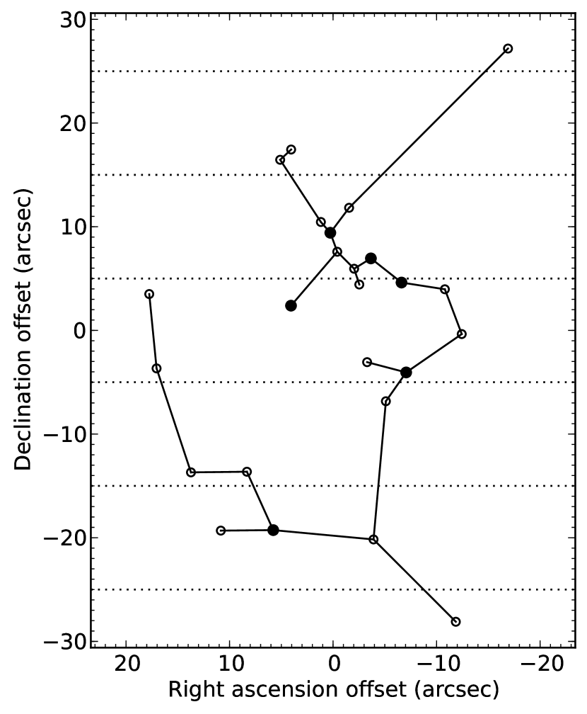
Following the techniques applied to infrared and optical observations of clusters of stars and HII regions (e.g. Pleuss et al., 2000; Schmeja & Klessen, 2006), we have constructed the minimal spanning tree (MST) formed from these 25 sources, as shown in Figure 10. The minimum spanning tree for a set of points is defined as the set of edges connecting them that possesses the smallest sum of edge lengths. To compute it, we used a python function based on the algorithm of Prim (1957). From this result, we compute the Q-parameter, which is defined as the ratio of $\bar{m}$, the normalized mean edge length of the MST, to $\bar{s}$, the correlation length, which is defined as the mean projected separation between sources normalized by the cluster radius, $R_{\rm cluster}$ (Cartwright & Whitworth, 2004). $R_{\rm cluster}$ is defined as the distance from the mean position of all the stars to the furthest star from that point. For this cluster, we obtain $R_{\rm cluster}=31.95\arcsec$ and:

$$Q=\frac{\bar{m}}{\bar{s}}=\frac{6.024\arcsec/\biggl{(}\frac{\sqrt{N_{\rm total}\pi R_{\rm cluster}^{2}}}{(N_{\rm total}-1)}\biggr{)}}{19.93\arcsec/R_{\rm cluster}}=\frac{0.510}{0.623}=0.82$$ (1)

Interestingly, this value (0.82) is close to the critical value that separates clusters between the regime of multiscale (fractal) substructure ($Q<0.8$) typified by the Taurus and Chamaeleon clusters, and a centrally concentrated configuration typified by $\rho$ Oph and IC348 (Cartwright & Whitworth, 2004). It is also close to the value of 0.84 obtained for stars in the Orion Trapezium Cluster (Kumar & Schmeja, 2007). In the smoothed particle hydrodynamics simulation of the formation of a 1000 $M_{\odot}$ cluster (Bonnell et al., 2003), the $Q$-parameter of the resulting stars evolves steadily from initial values of $\sim$0.5 to values greater than 1.1 (Maschberger et al., 2010). It passes the critical 0.8 value after about 1.8 free-fall times. These results suggest that our measured value for $Q$ for this protocluster is not a fixed property but may instead provide a measure of its age. However, we caution that our census of the cluster may be limited by the primary beam of the observations, i.e. the cluster may extend beyond this region in one or more directions. It is also limited in terms of sensitivity depth. Future more sensitive observations with a wider field of view are needed to improve the robustness of this result. In any case, it is likely that this protocluster exists in a stage when its ultimate structure is still to be determined.

4.3 Dynamical mass and relaxation time

Using the virial theorem, the dynamical mass of a stellar cluster can be estimated from the mean square velocity of its members (relative to their mean velocity) as originally performed on the globular cluster M92 by Wilson & Coffeen (1954). For the NGC 6334 I(N) protocluster, we compute the unbiased sample variance of the source-to-source LSR velocities: $\langle v_{\rm 1D}^{2}\rangle=(1/(N_{\rm src}-1))\Sigma(v_{\rm src}-\bar{v})^{2}$, by using the fitted velocities ($v_{\rm src}$) from the single-component CH₃CN spectral models of the $N_{\rm src}=6$ sources in Table 7 and their mean ($\bar{v}$). As seen in Figure 10, three of these sources lie in the central strip, two in the first pair of flanking strips, and one in the second pair of flanking strips. Thus, although small in number, these six sources provide a fair spatial sampling across the cluster. The H₂O maser emission provides a potential kinematic measurement for two additional sources: SMA 20 and H₂O-C4. However, H₂O masers typically span a broad range in velocity, and the centroid can vary widely from the LSR of the thermal gas (Urquhart et al., 2011), as is the case for SMA 18, which is detected in both CH₃CN and H₂O. Therefore we have chosen not to include these two sources in this analysis. The resulting value and uncertainty of the unbiased sample variance are $\langle v_{\rm 1D}^{2}\rangle=2.05\pm 1.29$ km² s^-2, where the uncertainty in the variance is the variance times $\sqrt{2/(N_{\rm src}-1)}$ (e.g. Casella & Berger, 2002). Assuming a random orientation of space velocities, the mean square three dimensional velocity is then $\langle v_{\rm 3D}^{2}\rangle=3\langle v_{\rm 1D}^{2}\rangle=6.15\pm 3.87$ km² s^-2. The proper effective distance to use in the virial theorem, $\bar{r}$, can be determined by numerical integration of the observed strip counts (Schwarzschild & Bernstein, 1955). In this case, the strip counts are the number of stars in each horizontal bin shown in Figure 10. We chose a bin width of 10″ as it provides seven bins, which is a good compromise between having too few bins and having too few sources per bin. Using equation 1 of Schwarzschild & Bernstein (1955), we obtain $\bar{r}=44.3\arcsec$, or 0.28 pc, yielding a dynamical mass estimate of $410\pm 260$ $M_{\odot}$. By comparison, the gas mass of NGC 6334 I(N) plus SM2 based on single-dish submillimeter continuum observations is $280$ $M_{\odot}$, assuming a uniform dust temperature of 30 K (Sandell, 2000), after scaling to the new distance of 1.3 kpc. Because the Sandell (2000) mass is based on Gaussian fits to these two sources, it is a lower limit to the total gas mass as it does not include the mass of the more extended material between them (see Figs. 1 & 2). Furthermore, the total gas mass is a lower limit to the total cluster mass because it does not include the mass of condensed (proto)stars. Considering these effects, the agreement between these two measurements is remarkable, and lends credence to the interpretation of the hot core velocity dispersion as tracing the dynamics of the protocluster. We note that the velocity dispersion $\sigma_{v}=\sqrt{\langle v_{1D}^{2}\rangle}={1.43}$ km s^-1 is in good agreement with the internal radial velocity dispersion of the Scorpius OB2 cluster (1.0-1.5 km s^-1) as measured by kinematic modelling of Hipparcos data (de Bruijne, 1999).

We next consider the relaxation time of the protocluster, which is based on the crossing time:

$$t_{\rm cross}=R_{\rm cluster}/v_{\rm 3D}=87000\mbox{ yr}.$$ (2)

Because the number of known protostars is still fairly small, the relaxation time (see e.g. Binney & Tremaine, 1987) is essentially the same:

$$t_{\rm relax}=t_{\rm crossing}\frac{N_{\rm total}}{8\ln(N_{\rm total})}=84000\mbox{ yr}.$$ (3)

Given the likelihood that the protostellar population continues below our sensitivity limit, this value should be considered an upper limit to the relaxation time. The low value of the $Q$-parameter suggests that the protocluster is dynamically young in the context of evolutionary simulations (Parker et al., 2014). However, the good agreement between the dynamical mass and the gas mass suggests that the protocluster has already persisted for one or more crossing times, which theory suggests is sufficient for dynamical mass segregation to occur (Bonnell & Davies, 1998). Although the number of detected objects is too small to apply a statistical estimate of mass segregation (Allison et al., 2009), the probable most massive source in the protocluster (SMA 1b) is by no measure located near the center of the distribution of members (see Figure 2). Therefore, we do not see any clear evidence for mass segregation.

4.4 Individual dust masses: circumstellar disks?

Our single-component LTE model fits (Table 7) have provided gas temperature and column density measurements for six of the sources. Given the high volume densities implied by these fits, we make the usual assumption that the dust temperature ($T_{dust}$) is well coupled to the gas temperature through collisions. To obtain gas mass estimates from the 1.3 mm dust emission, we follow the procedure of Brogan et al. (2009) using the dust mass opacity coefficient $\kappa_{\rm 1.3mm}=1$ cm² g^-1 appropriate for grains with ice mantles in regions of high gas density (10⁸ cm^-3) (Ossenkopf & Henning, 1994), and a gas to dust mass ratio of 100. In the sources that do not show CH₃CN emission, we have no temperature measurement. In these cases, we have assumed a range of temperatures that are fairly low (20–50 K), and compute the range of masses implied by the measured flux density. This temperature range encompasses both the typical temperature of gas surrounding young protostars prior to the hot core phase, as well as the expected mean temperature of gas in circumstellar disks around stars of type A3 – B5 (Natta et al., 2000). The masses were corrected for the dust opacity by comparing the observed brightness temperature to the assumed dust temperature ($\tau_{dust}=-\ln(1-T_{b}/T_{dust})$) and the correction factor is: $\tau_{dust}/(1-\exp(-\tau_{dust}))$. The resulting mass estimates for all sources are shown in Table 9, and for a subset of sources in Figure 9.

With the exception of SMA 1a,b,c,d, SMA 3, and SMA 9, the mass estimates are in the range of 0.2-2 $M_{\odot}$. These masses cover a range similar to the masses of dense cores in the Perseus molecular cloud (Kirk et al., 2006); however, the smallest Perseus objects have a typical diameter $\approx$5000 AU (20″ at 250 pc) in submillimeter continuum images (Kirk et al., 2007). Such objects would be nearly 4″ in diameter at the distance of NGC 6334 I(N). Therefore, the emission we are detecting must arise from structures that are an order of magnitude (or more) smaller, which includes circumstellar disks. The mass values are not as high as massive disk candidates (e.g. the 0.8-8$M_{\odot}$ of IRAS 20126+4104, Cesaroni et al., 2005), but they are an order of magnitude higher than the typical masses of circumstellar disks around low-mass stars, for example 0.005-0.14 $M_{\odot}$ in the Ophiuchus sample of Andrews et al. (2009). However, they are not too massive to be disks around intermediate mass stars. There are a number of examples of Herbig A stars with disk masses of $\sim$0.2$M_{\odot}$, such as Mac CH12 (Mannings & Sargent, 2000). Its 1.3 mm flux density of 44 mJy (Osterloh & Beckwith, 1995) would be 19 mJy at the distance of NGC 6334 I(N). A more massive example is SMA1 in G5.89-0.39, which appears to be an intermediate mass protostar with $\sim$1 $M_{\odot}$ of circumstellar material (Hunter et al., 2008). Thus, along with the lower mass population of disks around high-mass protostars (such as the 0.8 $M_{\odot}$ of AFGL2591 VLA3; van der Tak et al., 2006), we may also be detecting the most massive tip of the population of disks around intermediate-mass protostars in this protocluster.

Finally, in principle one can use the H₂ gas column density estimated from the dust column density to calculate the CH₃CN abundance, subject to the assumption that both tracers arise from the same volume of gas. In the case of SMA 1b, the fitted size of the dust emission (0.87″ at 1.3 mm and 0.47″ at 0.87 mm) is significantly larger than the modeled size of the CH₃CN emission region (0.38″), so this assumption is not valid. Nevertheless, proceeding with this uncertainty, the gas column density toward SMA 1b inferred from the dust emission is $1\times 10^{25}$ cm^-2, yielding an abundance estimate of $4\times 10^{-8}$. Similarly, for the next two brightest line sources (SMA 2 and SMA 4), we obtain abundances of $5\times 10^{-9}$ and $6\times 10^{-8}$. Given all the uncertainties, these values are in reasonable agreement with the assumed value of $1\times 10^{-8}$ (see § 3.2). Higher resolution observations are needed to obtain more accurate estimates of the molecular abundances via this method.

4.5 A candidate massive rotating disk in SMA 1b

The position angle of the velocity gradient in the molecular gas in SMA 1b ($-52\pm$5°) is equal to the position angle of the two-dimensional Gaussian model fit to the dust emission (Figure 5): $-52\pm$9°at 1.3 mm (Table 2) and $-51\pm$8°at 0.87 mm (Table 5). Furthermore, this position angle is 91° different from the position angle of $+39$° determined for the SiO 5-4 outflow (Brogan et al., 2009, also see Figure 8). This perpendicularity is heavily suggestive of a disk-outflow system. In a few of the lower temperature transitions, including HC₃N, OCS, and ¹³CS, emission extends beyond SMA 1b by up to an arcsecond along the outflow direction on one or both sides. This behavior is not expected from a compact disk. However, at these locations, the kinematic structure changes from a strong gradient to a narrower range of velocities, suggesting that these transitions are tracing an interaction of the outflow with ambient material near the disk.

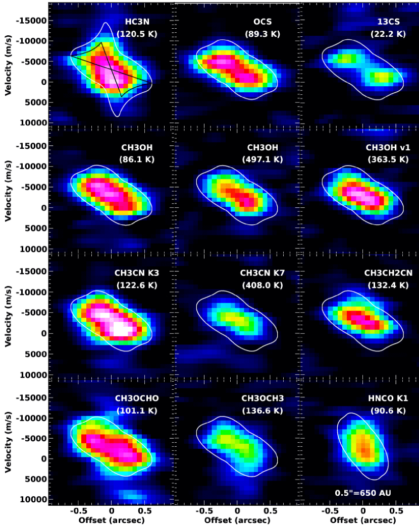
To further explore the velocity gradient toward SMA 1b, we constructed position-velocity (pv) images (Figure 11) for the same 12 transitions whose moment maps were shown in Figure 6 (the position and orientation of the slice is shown on the CH₃OCHO panel of Figure 6). In the context of a disk, three main factors will govern the appearance of the pv image of a molecular line: (1) the overall physical structure of the circum-protostellar material, in particular the outer radius, inner radius (if there is a central cavity), and the thickness; (2) the radial gradient in the temperature, density, and molecular abundance; and (3) the observer’s viewing angle. Evidence for chemical segregation in the context of a hot core was recently reported for the inner 3000 AU of the AFGL2591 VLA3, in which different species appear to trace different radii with respect to the continuum peak (Jiménez-Serra et al., 2012). One interpretation of this object is that it contains a massive disk (Hutawarakorn & Cohen, 2005; Trinidad et al., 2003). In the case of NGC 6334 I(N) SMA 1b, we observe the overall shapes of the structures in the pv images to be generally consistent with one another, but the differences are worth noting. In general, the high temperature transitions are peaked toward the central source, including the two highest temperature CH₃OH lines, CH₃CN K=7, and CH₃CH₂CN. In contrast, most of the lower temperature transitions show a double peak with a local minimum toward the central source, including ¹³CS, OCS, CH₃OCHO and CH₃CN K=3. This pattern is consistent with the combination of a radial temperature gradient in which the hotter gas lies closer to the central heating source, and a viewing angle that is edge-on (or at least moderately so). The two species that deviate from this picture are HNCO, which shows a distinctive compact morphology, and HC₃N, which extends to higher velocities.

Regarding HNCO, Tideswell et al. (2010) recently modelled its abundance in hot cores versus time using a wide range of assumed chemical reactions (both grain and gas-phase), along with different initial cloud collapse temperatures and post-collapse (hot core) temperatures. They find the best agreement with observed abundances from models that include both grain and gas-phase chemistry, cloud collapse temperatures of 10 K, and post-collapse temperatures $>50$ K. Furthermore, the late peak of HNCO abundance with time ($2\times\/10^{5}$ yr) suggests that HNCO is not itself a “first generation” species liberated from dust grains. Instead, it is the ejection of several larger HNCO “daughter” molecules formed on the grains (such as HNCOHO, HNCOCHO, HNCONH, and HNCOOH) and their subsequent destruction that form HNCO in the gas phase. The compact size of the observed HNCO emission relative to other species suggests that this formation scenario is efficiently proceeding only in the inner disk, perhaps due to the higher temperatures there.

Regarding HC₃N, not only does its emission extend to higher velocities, but these velocities arise exclusively from locations close to the center. This pattern suggests faster rotation toward the inner radii. However, it is somewhat surprising that HC₃N is seen closer to the central source than other molecules given that it has a relatively high photodissociation rate (Martín et al., 2012) and that ionizing radiation should be stronger at smaller radii. On the other hand, if there are locations with sufficient shielding, such as in the mid-plane of a high column density disk, the formation of HC₃N can proceed quickly as a product of C₂H₂ and CN (e.g. Meier & Turner, 2005; Fukuzawa & Osamura, 1997), and CN has a low photodissociation rate (Martín et al., 2012). It is interesting to note that the HC₃N abundance observed toward the continuum peak of AFGL2591 VLA3 by Jiménez-Serra et al. (2012) exceeds their gas-grain chemical evolution model predictions by more than two orders of magnitude. Indeed, these authors emphasize that molecular abundances are very sensitive to extinction, and hence the detailed geometry of the system.

As seen in Figure 11, the maximum extent of the emission toward SMA 1b is $\pm 0.6$″ ($\pm$800 AU) and the observed range of gas velocities at that radius is approximately $\pm 3.5$ km s^-1 with respect to the LSR. If this emission is interpreted as arising from a circular rotating disk, then these two quantities alone can be used to make a simple dynamical estimate of the central enclosed mass using Kepler’s law for circular rotation: $M_{\rm enclosed}=R(V/\sin i)^{2}/G=11/\sin^{2}i$ $M_{\odot}$, where $i$ is the angle of inclination of the rotation axis to the line of sight. However, rotation is not the only possible motion, as evidence for infall in this source has already been demonstrated by the trend of the increasingly redshifted absorption features with increasing line excitation seen in three transitions of CN and H₂CO (Brogan et al., 2009). Therefore, to build a more illustrative physical model, we follow the approach of Equation 1 of Cesaroni et al. (2011), where we interpret the pv images as arising from a rotating Keplerian disk undergoing free-fall and having a specific inner and outer radius. Using this model, the white contour in Figure 11 encompasses the entire region where emission can arise (ignoring any effects of line opacity and dust opacity) from a disk with an enclosed mass of $M_{\rm enclosed}=10/\sin^{2}i$ $M_{\odot}$, and the specified inner and outer radii for each transition. (For comparison, the model without free-fall is included as the black contour in the first panel of Figure 11.) The inner radius sets the total extent of the white contour along the velocity axis, while the outer radius sets its total extent along the position axis. Most of the molecular transitions are consistent with a model having an inner radius of 500 AU, and outer radius of 800 AU. The HC₃N line is more consistent with a smaller inner radius of $\sim$200 AU, while the HNCO line is more consistent with originating from a narrow range of inner radii (400-500 AU).

The outer radius of 800 AU seen in most species is comparable to the semi-major axis of the deconvolved Gaussian model of the continuum from SMA 1b, which is 660$\pm$33 AU at 1.3 mm (Table 2) and 403$\pm$20 AU at 0.87 mm (Table 5). For example, an outer radius of 800 AU for the molecular gas would correspond to the 7$\pm$2 percent point of the 0.87 mm model dust source. Thus, the extent of the dust and gas emission yield similar values for the size of the structure. Assuming circular symmetry, the observed ellipticity of the 0.87 mm deconvolved model can then be used to set a lower limit for $i$ of 55°, i.e. nearly edge-on. The corresponding upper limit for the enclosed mass is then 30 $M_{\odot}$. We note that for a disk viewed edge-on, the line emission from the innermost radii will be obscured by the high optical depth of the foreground material in the disk, both from the gas and (at some point) the dust grains. To demonstrate, the CH₃CN optical depths at line center for the $K$=7 and 8 components, derived from their peak brightness temperatures in the single-temperature CASSIS model, are 0.7 and 0.4, respectively. Although the presence of a Keplerian disk is tantalizing, future higher resolution observations are necessary to properly model the geometry and inclination angle and to confirm the expected kinematic structure in more detail. Radiative transfer modelling will no doubt be profitable in delineating and interpreting the chemical structure as it has been for low-mass protostellar disks (Qi et al., 2008).

5 Conclusions

Using new high-resolution SMA and VLA images from 6 cm to 0.87 mm, we have found further multiplicity in NGC 6334 I(N), allowing us to perform the first structural analysis of a massive protocluster using techniques developed for optical/infrared studies of star clusters. We also demonstrate the first use of the thermal gas velocities from an ensemble of hot cores to probe the dynamical properties of a protocluster. Our results are summarized as follows:

• We have identified 16 new compact 1.3 mm continuum sources and two new 6 cm sources. Three of the newly discovered sources are associated with H₂O masers. Combined with the previously-known 1.3 mm sources from Brogan et al. (2009), the total number of compact centimeter or millimeter sources is 28. Limiting our analysis to likely protostars, i.e. 25 sources (see § 4.2), we measure a protostellar density of $\sim 700$ pc^-3 and a minimum spanning tree $Q$-parameter of 0.82. Although our measurement of the $Q$-parameter is likely limited in terms of sensitivity and extent, the value is close to the expected value for a uniform volume density of sources.

• All nine sources detected at more than one continuum wavelength have SEDs indicative of dust emission. The long wavelength emission toward SMA 1b and SMA 4 is well modeled by the additional presence of a HCHII region. Thermal molecular line emission is detected towards six of the 1.3 mm continuum sources (SMA1b, SMA2, SMA4, SMA6, SMA15, and SMA18). From LTE modeling of CH₃CN ($J$=12-11) using CASSIS we find gas temperatures ranging from 95-373 K, CH₃CN column densities from (4-40)$\times 10^{16}$ cm^-2, and H₂ gas densities of (0.8-9)$\times 10^{8}$ cm^-3 (assuming a CH₃CN:H₂ abundance of $1\times 10^{-8}$). The radial velocities of the hot cores, measured from CH₃CN, range from $-3.3$ to $-7.0$ km s^-1, and the corresponding 1D velocity dispersion of 1.43 km s^-1 implies a dynamical mass of $410\pm 260$ $M_{\odot}$. This mass is compatible with the gas mass of $\sim 280$ $M_{\odot}$ based on single dish imaging, and demonstrates that hot core line emission can be an important probe of protocluster dynamics.

• The dominant hot core SMA 1b shows a consistent spatial-velocity structure in a wide range of hot core molecular lines that is consistent with a disk undergoing Keplerian rotation and free-fall. The orientation of the disk is in excellent agreement with the major axis of the dust continuum emission, and is perpendicular to the large scale outflow axis. The outer radius of the disk is $\sim$800 AU, and the enclosed mass is $\sim$10 - 30 $M_{\odot}$ (depending on the inclination angle). The radial distribution of HNCO and HC₃N appears to differ from the rest of the molecules.

• Nine positions in the protocluster exhibit 229.7588 GHz Class I methanol maser emission, generally in close proximity to previously-identified 44 GHz or 24.9 GHz Class I masers. The brightest position also exhibits 218.4400 GHz Class I methanol maser emission. These are the first observations with sufficient angular resolution to directly establish maser activity in these transitions (by demonstrating brightness temperatures in excess of their excitation energies).

Table 1: Parameters of new observations

Parameter	SMA 1.3 mm	SMA 0.87 mm	VLA 6 cm
Observing date	23 Feb 2010	18 Feb 2010	07 Jul 2011
On-source time	240 minutes	210 minutes	84 minutes
Project code	2009B-S036	2009B-S036	10C-186
Antennas	7	6	27
Configuration	very extended (VEX)	very extended (VEX)	A
Projected baseline lengths	28 m – 508 m	26.5 m – 508 m	0.53 km – 36.63 km
J2000 phase center	17:20:55.0, -35:45:07.0	17:20:55.0, -35:45:07.0	17:20:53.33, -35:46:00.0
Primary beam FWHM	53″	34″	9.5′, 6.8′
Synthesized beam	0.68″$\times$0.44″ (+5°)	0.55″$\times$0.26″ (+9°)	0.90″$\times$0.30″ (-2°)
Synthesized beam (EXT+VEX)	0.70″$\times$0.39″ (+5°)	…	…
Synthesized beam (VEX-UV)	0.66″$\times$0.36″ (+5°)	0.66″$\times$0.36″ (+5°)	…
Lower band center	218.85 GHz	335.54 GHz	5.06 GHz
Upper band center	230.83 GHz	347.54 GHz	7.16 GHz
Bandwidth	4 $\times$ 1.968 GHz	4 $\times$ 1.968 GHz	2 $\times$ 1.024 GHz
Subbands	4 $\times$ 24	4 $\times$ 24	2 $\times$ 8
Polarization	single linear	single linear	dual circular
Channel spacing	1.1 km s-1	0.7 km s-1	60 km s-1, 43 km s-1
Continuum rms noise (EXT+VEX)	2.2 mJy beam-1	8.7 mJy beam-1	18, 27 $\mu$Jy beam-1
Spectral line rms noise	30 mJy beam-1	130 mJy beam-1	…
Gain calibrator(s)	J1733-1304, J1924-2914	J1733-1304, J1924-2914	J1717-3342
Bandpass calibrator	3C273	3C273	J1924-2914
Flux calibrator(s)	Titan, Ceres	Ceres	J1331+3030
225 GHz zenith opacity	0.07	0.03-0.06	n/a
Median wind speed	2 m/s	5 m/s	3 m/s

Table 2: Observed properties of the 1.3 mm continuum sources

	Fitted Position (J2000)		Peak intensity	Peak	Fitted flux	Fitted size (Pos. angle E of N)	Fitted size	Tbrightness
Source	$\alpha$ (${}^{\rm h}~{}~{}^{\rm m}~{}~{}^{\rm s}$)	$\delta$ (${}^{\circ}~{}~{}{{}^{\prime}}~{}~{}{{}^{\prime\prime}}$)	(Jy beam-1)	S/N	density (Jy)	${{}^{\prime\prime}}\times{{}^{\prime\prime}}$ (°)	(AU)	(K)
SMA 1a	17:20:55.137	-35:45:05.76	0.0866 $\pm$0.0022	39	0.225$\pm$0.020	0.99$\pm$0.05 $\times$ 0.52$\pm$0.10 (+35$\pm$5)	1300$\times$680	10$\pm$2
SMA 1b+d	17:20:55.192	-35:45:03.93	0.3257 $\pm$0.0022	148	1.059$\pm$0.076	1.02$\pm$0.05 $\times$ 0.74$\pm$0.06 (+128$\pm$9)	1300$\times$960	32$\pm$4
SMA 1c	17:20:55.267	-35:45:02.89	0.1384 $\pm$0.0022	63	0.335$\pm$0.024	0.74$\pm$0.05 $\times$ 0.61$\pm$0.07 (+141$\pm$25)	960$\times$790	17$\pm$3
SMA 2	17:20:54.870	-35:45:06.40	0.1039 $\pm$0.0022	47	0.169$\pm$0.007	0.58$\pm$0.03 $\times$ 0.27$\pm$0.07 (+138$\pm$6)	750$\times$350	24$\pm$6
SMA 3	17:20:55.003	-35:45:07.40	0.0331 $\pm$0.0022	15	0.138$\pm$0.016	1.06$\pm$0.06 $\times$ 0.93$\pm$0.09 (+10$\pm$25)	1400$\times$1200	3.2$\pm$0.5
SMA 4	17:20:54.627	-35:45:08.73	0.0425 $\pm$0.0022	19	0.059$\pm$0.004	$<0.5$	$<650$	$>5.4$
SMA 5	17:20:55.043	-35:45:01.53	0.0433 $\pm$0.0022	20	0.053$\pm$0.002	0.68$\pm$0.01 $\times$ 0.51$\pm$0.03 (+6$\pm$1)	890$\times$660	4.9$\pm$0.3
SMA 6	17:20:54.590	-35:45:17.40	0.1812 $\pm$0.0022	82	0.285$\pm$0.016	$<0.5$	$<650$	$>26$
SMA 7	undetected	…	…	…	…	…	…
SMA 8	17:20:53.782	-35:44:46.16	0.0297 $\pm$0.0034	8.7	0.046$\pm$0.003	$<0.5$	$<650$	$>4.4$
SMA 9	17:20:54.196	-35:45:41.45	0.1070 $\pm$0.0054	20	0.139$\pm$0.006	$<0.5$	$<650$	$>13$
SMA 10	17:20:54.283	-35:45:09.38	0.0115 $\pm$0.0022	5.2	0.025$\pm$0.003	$<0.5$	$<650$	$>2.2$
SMA 11	17:20:54.751	-35:45:20.18	0.0197 $\pm$0.0022	9.0	0.043$\pm$0.004	0.72$\pm$0.07 $\times$ 0.27$\pm$0.15 (+76$\pm$25)	940$\times$350	5.0$\pm$2.5
SMA 12	17:20:54.849	-35:45:33.51	0.0312 $\pm$0.0034	9.2	0.039$\pm$0.004	$<0.5$	$<650$	$>3.5$
SMA 13	17:20:54.900	-35:45:16.41	0.0425 $\pm$0.0022	19	0.049$\pm$0.004	$<0.5$	$<650$	$>4.4$
SMA 14	17:20:54.962	-35:45:08.92	0.0130 $\pm$0.0022	5.9	0.022$\pm$0.002	0.49$\pm$0.09 $\times$ 0.39$\pm$0.11 (+104$\pm$25)	640$\times$510	2.7$\pm$0.9
SMA 15	17:20:55.504	-35:45:10.96	0.0469 $\pm$0.0022	21	0.063$\pm$0.003	$<0.5$	$<650$	$>5.8$
SMA 16	17:20:55.503	-35:44:55.90	0.0179 $\pm$0.0022	8.1	0.031$\pm$0.004	$<0.5$	$<650$	$>2.8$
SMA 17	17:20:55.590	-35:44:56.89	0.0145 $\pm$0.0022	6.6	0.021$\pm$0.003	$<0.5$	$<650$	$>1.9$
SMA 18	17:20:55.645	-35:45:32.61	0.0433 $\pm$0.0034	13	0.043$\pm$0.003	$<0.5$	$<650$	$>3.9$
SMA 19	17:20:55.854	-35:45:26.98	0.0179 $\pm$0.0025	7.2	0.024$\pm$0.004	$<0.5$	$<650$	$>2.1$
SMA 20	17:20:56.061	-35:45:32.66	0.0320 $\pm$0.0034	9.4	0.032$\pm$0.003	$<0.5$	$<650$	$>2.4$
SMA 21	17:20:56.298	-35:45:27.04	0.0362 $\pm$0.0034	11	0.052$\pm$0.004	$<0.5$	$<650$	$>4.7$
SMA 22	17:20:56.571	-35:45:17.01	0.0263 $\pm$0.0025	11	0.042$\pm$0.003	0.58$\pm$0.05 $\times$ 0.31$\pm$0.10 (+2$\pm$4)	750$\times$400	5.5$\pm$1.9
SMA 23	17:20:56.629	-35:45:09.84	0.0167 $\pm$0.0025	6.7	0.017$\pm$0.002	$<0.5$	$<650$	$>1.5$

Table 3: Observed properties of the 6 centimeter continuum sources

	Fitted Position (J2000)		Peak intensity (mJy beam-1)
Source	$\alpha$ (${}^{\rm h}~{}~{}^{\rm m}~{}~{}^{\rm s}$)	$\delta$ (${}^{\circ}~{}~{}{{}^{\prime}}~{}~{}{{}^{\prime\prime}}$)	5.06 GHz	7.16 GHz
SMA 1b	17 20 55.192	-35 45 03.83	0.327$\pm$0.014	0.373$\pm$0.019
SMA 4	17 20 54.619	-35 45 08.57	0.157$\pm$0.014	0.235$\pm$0.026
H2O-C4	17 20 54.149	-35 45 13.70	0.110$\pm$0.011	0.091$\pm$0.019
VLA 2	17 20 54.871	-35 45 36.49	0.102$\pm$0.014	0.133$\pm$0.041

Table 4: Revised positions of the 1.3 and 0.7 centimeter continuum sources

	Fitted Position (J2000)
Source	$\alpha$ (${}^{\rm h}~{}~{}^{\rm m}~{}~{}^{\rm s}$)	$\delta$ (${}^{\circ}~{}~{}{{}^{\prime}}~{}~{}{{}^{\prime\prime}}$)
1.3 Centimeter
SMA 1b	17 20 55.185	-35 45 03.98
SMA 1c	17 20 55.259	-35 45 02.88
SMA 1d	17 20 55.222	-35 45 04.08
SMA 4	17 20 54.616	-35 45 08.66
0.7 Centimeter
SMA 1a	17 20 55.150	-35 45 05.71
SMA 1b	17 20 55.190	-35 45 03.95
SMA 1c	17 20 55.255	-35 45 02.91
SMA 1d	17 20 55.223	-35 45 04.12
VLA 3	17 20 54.992	-35 45 06.92
SMA 4	17 20 54.618	-35 45 08.71
SMA 6	17 20 54.591	-35 45 17.39

Table 5: Observed properties of the 0.87 mm continuum sources

	Fitted Position (J2000)		Peak intensity	Fitted flux	Fitted size (Pos. angle E of N)	Fitted size	Tbrightness
Source	$\alpha$ (${}^{\rm h}~{}~{}^{\rm m}~{}~{}^{\rm s}$)	$\delta$ (${}^{\circ}~{}~{}{{}^{\prime}}~{}~{}{{}^{\prime\prime}}$)	(Jy beam-1)	density (Jy)	${{}^{\prime\prime}}\times{{}^{\prime\prime}}$ (°)	(AU)	(K)
SMA 1c	17:20:55.269	-35:45:02.88	0.296$\pm$0.014	0.63$\pm$0.03	0.63$\pm$0.03 $\times$ 0.42$\pm$0.05 (+113$\pm$10)	820$\times$550	24$\pm$3
SMA 1b+d	17:20:55.194	-35:45:03.98	0.801$\pm$0.014	1.67$\pm$0.08	0.62$\pm$0.03 $\times$ 0.36$\pm$0.06 (+129$\pm$8)	810$\times$470	76$\pm$14
SMA 2	17:20:54.871	-35:45:06.43	0.230$\pm$0.014	0.27$\pm$0.02	0.64$\pm$0.03 $\times$ 0.43$\pm$0.04 (+164$\pm$2)	830$\times$560	9.9$\pm$1.2
SMA 4	17:20:54.626	-35:45:08.73	0.125$\pm$0.015	0.13$\pm$0.02	0.65$\pm$0.02 $\times$ 0.38$\pm$0.04 (+178$\pm$2)	850$\times$490	5.4$\pm$0.7
SMA 5	17:20:55.048	-35:45:01.42	0.061$\pm$0.016	0.06$\pm$0.02	$<0.5$	$<650$	$>3.5$
SMA 6	17:20:54.595	-35:45:17.40	0.461$\pm$0.020	0.66$\pm$0.04	$<0.5$	$<650$	$>41$
SMA 13	17:20:54.883	-35:45:16.32	0.107$\pm$0.018	0.28$\pm$0.03	$<0.5$	$<650$	$>17$
SMA 15	17:20:55.511	-35:45:11.07	0.107$\pm$0.016	0.19$\pm$0.04	$<0.5$	$<650$	$>12$

Table 6: Properties of spectral lines shown in Figure 6.

Species	Transition	Frequency	$E_{lower}$		Integrated Intensity (Jy beam-1*km s-1)
		(GHz)	(K)	Catalog	SMA1b	SMA2	SMA4	SMA6	SMA15	SMA18
HC3N	J=24–23	218.32479	120.5	JPL	7.49 $\pm$ 0.22	$<$0.65	2.48 $\pm$ 0.22	1.52 $\pm$ 0.38	$<$0.74	2.90 $\pm$ 0.41
OCS	J=18–17	218.90336	89.3	CDMS	4.71 $\pm$ 0.21	1.38 $\pm$ 0.21	2.64 $\pm$ 0.21	2.03 $\pm$ 0.28	0.6 $\pm$ 0.2	2.36 $\pm$ 0.36
13CS	J=5–4	231.22069	22.2	CDMS	2.06 $\pm$ 0.30	1.22 $\pm$ 0.30	2.06 $\pm$ 0.30	1.02 $\pm$ 0.29	$<$0.70	$<$1.54
CH3OH ($E$)	80,8–71,6	220.07849	86.1	CDMS	5.45 $\pm$ 0.33	3.16 $\pm$ 0.33	4.48 $\pm$ 0.33	2.04 $\pm$ 0.32	$<$0.79	$<$1.27
CH3OH ($E$)	201,19–200,20	217.88639	497.9	CDMS	3.68 $\pm$ 0.22	1.07 $\pm$ 0.22	2.63 $\pm$ 0.22	$<$0.86	$<$0.84	$<$1.31
CH3OH vt=1 ($A$)	61,5–72,6	217.29920	363.5	CDMS	4.40 $\pm$ 0.28	1.61 $\pm$ 0.28	3.47 $\pm$ 0.28	$<$0.87	$<$0.86	$<$1.72
CH3CN	J=12–11, K=3	220.70902	122.6	JPL	6.08 $\pm$ 0.27	2.56 $\pm$ 0.27	3.29 $\pm$ 0.27	1.87 $\pm$ 0.35	$<$0.80	2.63 $\pm$ 0.39
CH3CN	J=12–11, K=7	220.53932	408.0	JPL	2.63 $\pm$ 0.22	$<$0.65	$<$0.65	$<$0.74	$<$0.49	$<$1.08
CH3CH2CN	252,24–242,23	220.66092	132.4	CDMS	4.34 $\pm$ 0.29	$<$0.88	$<$0.88	$<$0.71	$<$0.66	$<$1.18
CH3OCHO ($A$)	201,20–191,19	216.96590	101.1	JPL	5.75 $\pm$ 0.28	4.34 $\pm$ 0.28	2.53 $\pm$ 0.28	2.03 $\pm$ 0.35	$<$0.99	$<$1.52
CH3OCH3	172,15–163,14	230.23376	136.6	JPL	3.19 $\pm$ 0.23	1.23 $\pm$ 0.23	1.06 $\pm$ 0.23	$<$0.72	$<$0.63	$<$1.25
HNCO	101,10–91,9	218.98101	90.6	CDMS	5.28 $\pm$ 0.23	2.13 $\pm$ 0.23	2.07 $\pm$ 0.23	0.85 $\pm$ 0.27	$<$0.89	$<$1.44

Table 7: Best fit CASSIS LTE models to the CH₃CN spectra

	Temperature	Diameter		Column density	Linewidth	LSR velocity	H2 Density
Source	(K)	(″)	(AU)	(cm-2)	(km s-1)	(km s-1)	(cm-3)
One-component models
SMA 1b	143$\pm$7	0.38$\pm$0.01	490	(3.94$\pm$0.34)E17	4.72$\pm$0.01	-3.29$\pm$0.01	8E9
SMA 2	140$\pm$6	0.30$\pm$0.01	390	(4.26$\pm$0.72)E16	4.40$\pm$0.07	-7.01$\pm$0.02	1E9
SMA 4	208$\pm$2	0.26$\pm$0.01	340	(6.26$\pm$0.20)E16	8.79$\pm$0.04	-6.80$\pm$0.02	2E9
SMA 6	95$\pm$3	0.25$\pm$0.01	330	(9.39$\pm$0.32)E16	4.26$\pm$0.15	-4.91$\pm$0.10	3E9
SMA 15	72$\pm$15	0.22$\pm$0.03	290	(3.76$\pm$0.46)E16	3.76$\pm$0.46	-6.36$\pm$0.37	1E9
SMA 18	139$\pm$10	0.25$\pm$0.02	330	(4.77$\pm$0.51)E16	5.71$\pm$0.36	-4.94$\pm$0.16	1E9
Two-component models
SMA 1b comp. 1	80$\pm$5	0.40$\pm$0.02	520	(4.51$\pm$0.31)E17	3.21$\pm$0.15	-3.24$\pm$0.17	9E9
SMA 1b comp. 2	307$\pm$40	0.24$\pm$0.02	310	(2.89$\pm$0.27)E17	6.63$\pm$0.52	-3.35$\pm$0.17	9E9
SMA 4 comp. 1	135$\pm$5	0.30$\pm$0.01	390	(3.06$\pm$0.25)E16	4.78$\pm$0.66	-8.25$\pm$0.07	8E8
SMA 4 comp. 2	280$\pm$35	0.22$\pm$0.02	290	(3.31$\pm$0.51)E16	6.85$\pm$0.38	-2.67$\pm$0.19	1E9

Table 8: Observed and derived parameters of the 218 and 229 GHz CH₃OH maser emission

	Fitted Position (J2000)		Peak intensity	Flux density	Deconvolved	$T_{\rm B}$	$v_{\rm LSR}$
Component	$\alpha$ (${}^{\rm h}~{}~{}^{\rm m}~{}~{}^{\rm s}$)	$\delta$ (${}^{\circ}~{}~{}{{}^{\prime}}~{}~{}{{}^{\prime\prime}}$)	(Jy/beam)	(Jy)	size (″$\times$ ″)	(K)	(km s-1)
229.75881 GHz (8-1,8-70,7) E transition
1 (8)	17 20 54.327	-35 45 22.31	0.76	$1.51\pm 0.12$	$<0.5$	145	$-7.56\pm 0.06$
2 (9)	17 20 54.392	-35 45 22.68	0.57	$1.91\pm 0.13$	$<0.5$	180	$-8.66\pm 0.13$
3 (11)	17 20 54.447	-35 45 22.76	1.46	$3.19\pm 0.15$	$0.67\times 0.23$	480	$-7.65\pm 0.07$
4	17 20 54.589	-35 45 10.33	0.79	$2.18\pm 0.22$	$0.80\times 0.42$	150	$-2.66\pm 0.06$
5 (22)	17 20 54.925	-35 45 13.70	1.25	$1.45\pm 0.18$	$<0.5$	$>140$	$-5.56\pm 0.06$
6 (25)	17 20 54.952	-35 45 13.99	0.84	$1.98\pm 0.11$	$0.82\times 0.15$	380	$-5.15\pm 0.07$
7	17 20 55.048	-35 45 14.89	0.76	$0.84\pm 0.06$	$0.39\times 0.12$	420	$-5.73\pm 0.08$
8	17 20 55.024	-35 45 15.32	0.60	$1.60\pm 0.07$	$0.82\times 0.42$	110	$-5.15\pm 0.06$
9 (55)	17 20 55.670	-35 45 00.38	6.40	$8.80\pm 0.16$	$0.44\times 0.15$	3100	$-3.03\pm 0.01$
218.44005 GHz ($4_{2,2}$-$3_{1,2}$) E transition
9 (55)	17 20 55.671	-35 45 00.34	2.28	$3.09\pm 0.12$	$<0.5$	270	$-3.07\pm 0.03$

Table 9: Gas properties derived from the dust emission

	Temperature range	Mass range	Column density range
Source	(K)	($M_{\odot}$)	(1024 cm-2)
SMA 1a	20 – 50	2.2 – 15	4.8 – 33
SMA 1b	143$\pm$7	4.3$\pm$1.1	1.0$\pm$0.2
SMA 1c	20 – 50	3.5 – 31	9.6 – 92
SMA 1d	20 – 50	0.4 – 2.2	1.9 – 11
SMA 2	140$\pm$6	0.71$\pm$0.18	8.1$\pm$2.7
SMA 3	20 – 50	1.2 – 6.5	1.5 – 8.1
SMA 4	208$\pm$2	0.15$\pm$0.03	1.1$\pm$0.2
SMA 5	20 – 50	0.5 – 2.5	1.8 – 8.5
SMA 6	95$\pm$3	2.0$\pm$0.5	1.4$\pm$0.3
SMA 8	20 – 50	0.4 – 2.2	2.1 – 10
SMA 9	20 – 50	1.4 – 11	7.3 – 46
SMA 10	20 – 50	0.2 – 1.1	1.1 – 5.5
SMA 11	20 – 50	0.4 – 2.2	1.5 – 16
SMA 12	20 – 50	0.4 – 1.8	1.7 – 8.8
SMA 13	20 – 50	0.5 – 2.4	2.3 – 11
SMA 14	20 – 50	0.2 – 1.0	1.0 – 7.3
SMA 15	72$\pm$15	0.50$\pm$0.16	3.6$\pm$0.8
SMA 16	20 – 50	0.3 – 1.5	1.4 – 6.9
SMA 17	20 – 50	0.2 – 1.0	1.3 – 6.6
SMA 18	139$\pm$10	0.17$\pm$0.04	1.2$\pm$0.3
SMA 19	20 – 50	0.2 – 1.1	1.0 – 5.4
SMA 20	20 – 50	0.3 – 1.5	1.4 – 7.1
SMA 21	20 – 50	0.5 – 2.5	2.4 – 12
SMA 22	20 – 50	0.4 – 2.2	2.1 – 16
SMA 23	20 – 50	0.2 – 0.8	0.7 – 3.6

Figure 1: Overview of the NGC6334 I(N) region in the mid-infrared. The three-color image was generated from the Spitzer MIPSGAL and GLIMPSE survey images at 24, 4.5, and 3.6 µm (Benjamin et al., 2003; Churchwell et al., 2009; Carey et al., 2009). For reference the SMA compact + extended (COMP+EXT) configuration 1.3 mm continuum with $2.2\arcsec\times 1.3\arcsec$ resolution from Brogan et al. (2009) is shown in white contours (levels=40, 80, 160, 320, 640 mJy beam^-1). The dashed yellow contours show the JCMT 0.45 mm emission ($14^{\prime\prime}$ resolution) from Sandell (2000) (levels: 60, 80, 100, 120, 160 Jy beam^-1). The labeled 0.45 mm contour indicates the position of the single-dish source SM2 reported by Sandell (2000).

Figure 2: SMA 1.3 mm EXT+VEX continuum with $0.7\arcsec\times 0.39\arcsec$ resolution in greyscale and a single black solid contour at $4.5\sigma\/=10$ mJy beam^-1. The dotted circle marks the 25% level of the southern edge of the primary beam–although we searched for sources out to 20% level, none were found beyond this radius. The labels correspond to the source names in Tables 2 and 3. The image used in this figure was not corrected for the primary beam response, but all measurements, including Table 2, were taken from the corrected image. The JVLA 6 cm continuum data is shown as a single red contour at 80 $\mu$Jy beam^-1(4.5$\sigma$). For ease of comparison with previous work and Fig. 1, the single dashed blue contour shows the 40 mJy beam^-1 level of the COMP+EXT SMA 1.3 mm continuum and the dashed yellow contour shows the 60 and 100 Jy beam^-1 levels of the JCMT 0.45 mm continuum. The green crosses mark the H₂O masers from Brogan et al. (2009).

Figure 3: Zoom on the central portion of the NGC 6334 I(N) protocluster including SMA1, SMA2, SMA3, and SMA4. The SMA 1.3 mm EXT+VEX continuum image is in greyscale and black contours (levels: 10, 24, and 66 mJy beam^-1). The red contours are the 6 cm VLA image (levels: 80, 144, and 200 $\mu$Jy beam^-1). The blue contours show the 7 mm VLA continuum (levels: 0.63, and 0.84 mJy beam^-1). The yellow contours show the 1.3 cm VLA continuum (levels: 0.23, and 0.35 mJy beam^-1). The green crosses mark the centroid positions of H₂O masers from Brogan et al. (2009). The synthesized beams are shown in the lower left corner coded by contour color, the 7 mm beam is not shown as it is very similar to the SMA 1.3 mm beam (black) (see Table 1).

Figure 4: Zoom on the SMA 6 region. The SMA 1.3 mm EXT+VEX continuum image is shown in greyscale and black contours (levels: 10 ($4.5\sigma$), 24, 66 mJy beam^-1). The magenta contours show the tapered and convolved (to match 1.3 mm) SMA VEX 0.87 mm continuum (levels: 75 ($3\sigma$ at this point in the primary beam), 150, and 300 mJy beam^-1). The blue contours show the 7 mm VLA continuum (levels: 0.63 ($3\sigma$) and 95 mJy beam^-1). The green crosses mark the centroid positions of the three groups of H₂O masers from Brogan et al. (2009). The synthesized beams are shown in the lower left coded by contour color; the 1.3 mm and 0.87 mm resolutions are the same (black).

Figure 5: (a) The SMA 1.3 mm VEX-UV continuum image is in greyscale, and the colored crosses mark the positions and velocities of H₂O masers from Brogan et al. (2009). (b) The velocity field (moment 1) of the CH₃CN $J$=12–11, $K$=7 line is shown in colorscale, and the fitted positions of the 1.3 cm continuum emission (Table 4) are marked by stars. In both panels, the native resolution VEX 0.87 mm continuum image is shown by solid magenta contours (levels: 60, 120, 240 mJy beam^-1) and the 7 mm continuum emission is shown by dashed blue contours (levels: 0.63 and 0.84 mJy beam^-1).

Figure 6: Images of the first moment of the 12 spectral lines listed in Table 6 from the SMA VEX 1.3 mm data. The field of view is the same as Figure 3. The excitation energy (in Kelvin) of the lower level of each transition is indicated. The black contours show the 1.3 mm EXT+VEX continuum emission (contour levels: 10, 24, and 66 mJy beam^-1). The arrow in the lower left panel indicates the cut used to generate the pv diagrams in Figure 11. The resolution of the EXT+VEX continuum and VEX line data is similar (see Table 1); the beamsize is shown in the lower left corner of the lower left panel.

Figure 7: In each panel, the black spectrum is the observed spectrum toward the indicated source in units of brightness temperature (corrected for primary beam response), and the red spectrum is the best fit single-component CASSIS LTE model of CH₃CN and CH${}_{3}^{13}$CN $J$= 12–11. The blue spectrum shown for SMA 1b and SMA 4 is a two component model. The corresponding model parameters are given in Table 7. In the SMA 1b panel, the vertical lines below the spectrum mark the frequencies of the $K$ components of CH₃CN (solid lines) and CH${}_{3}^{13}$CN (dotted lines). The rest frequency of ¹³CO is also marked by the vertical dashed line. The flat tops on many of the low $K$ lines are indicative of high optical depths.

Figure 8: Image of the EXT+VEX 1.3 mm continuum in greyscale and black contours, (same three contours as in Figure 3). The field of view is identical to Figure 2. The integrated intensity of the SiO $J$=5–4 emission from the COMP+EXT SMA data presented in Brogan et al. (2009) is shown in gray contours, indicating strong outflow emission. The positions of the various CH₃OH masers are marked as follows: $\times$: 229.76 GHz; square: 218.44 GHz; $+$: 44 GHz; diamond: 24.9 GHz (Beuther et al., 2005); 5-pointed star: the intensity-weighted centroid of the six 6.7 GHz masers (17:20:54.619, -35:45:08.66) computed from the table in Walsh et al. (1998). The positions and velocities of the newly discovered Class I 218.44 and 229.76 GHz CH₃OH masers are tabulated in Table 8.

Figure 9: The spectral energy distributions of the nine continuum sources detected at more than one wavelength. The 6 cm, 1.3 mm and 0.87 mm measurements are from this paper, while the rest can be found in Brogan et al. (2009). The flux density error bars represent the formal error of the two-dimensional Gaussian model fit plus a fraction of the total flux density (to account for the typical calibration uncertainty, see § 2). Non-detections are shown as 3 $\sigma$ upper limits. The 3 mm flux density measurements for SMA 4 and SMA 6 (Brogan et al., 2009) are regarded as upper limits for the size scales considered here. The lower limits drawn for the detections at 0.87 mm are due to the relative lack of short spacings compared to the 1.3 mm measurements. In SMA 1b and SMA 4, the dotted curve is a free-free emission model ($n_{e}\propto r^{-2}$: Olnon, 1975) whose parameters are listed in the lower right, the dashed curve is the dust model, and the solid curve is the sum. The parameters of the dust emission model are listed in the upper left of each panel. For SMA 1c, 1d, 5, and 13, the dashed and dotted curves are $T$=50 K and $T$=20 K dust, respectively.

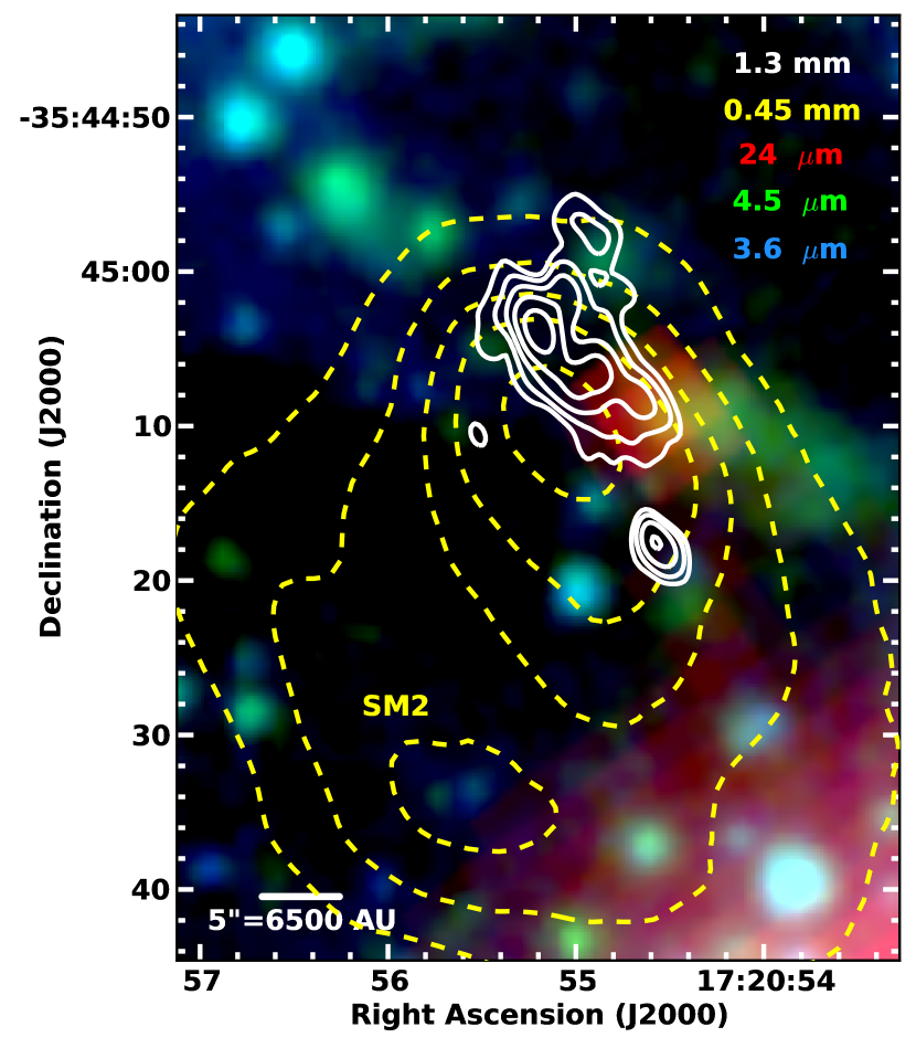
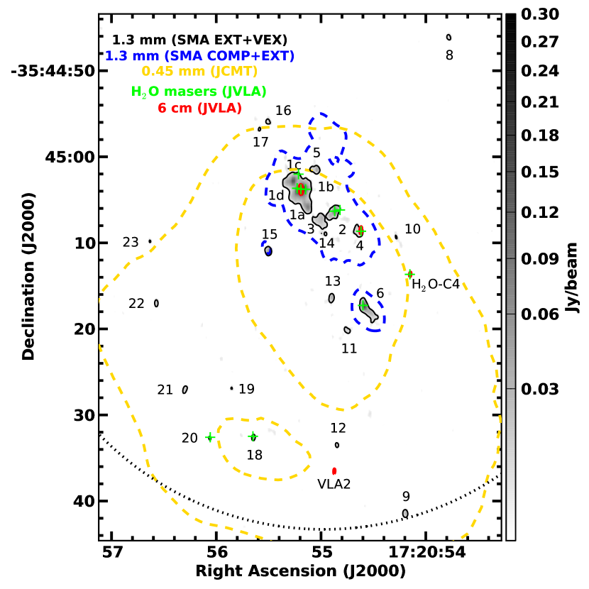
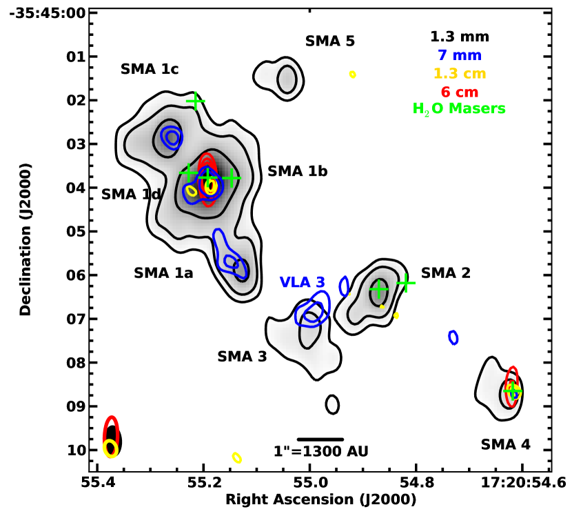
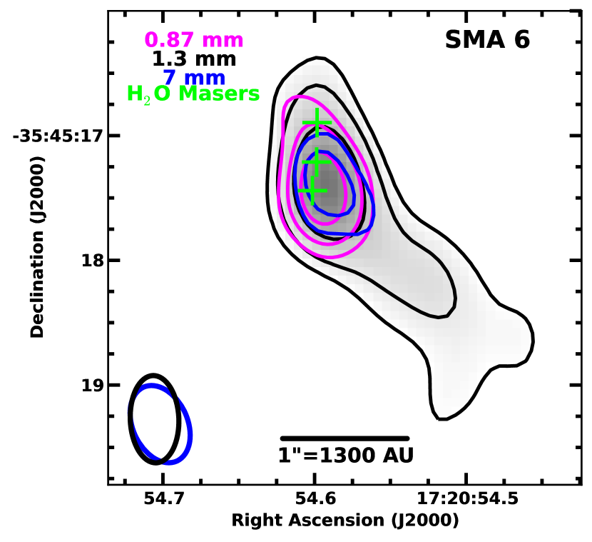
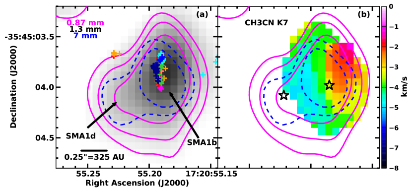
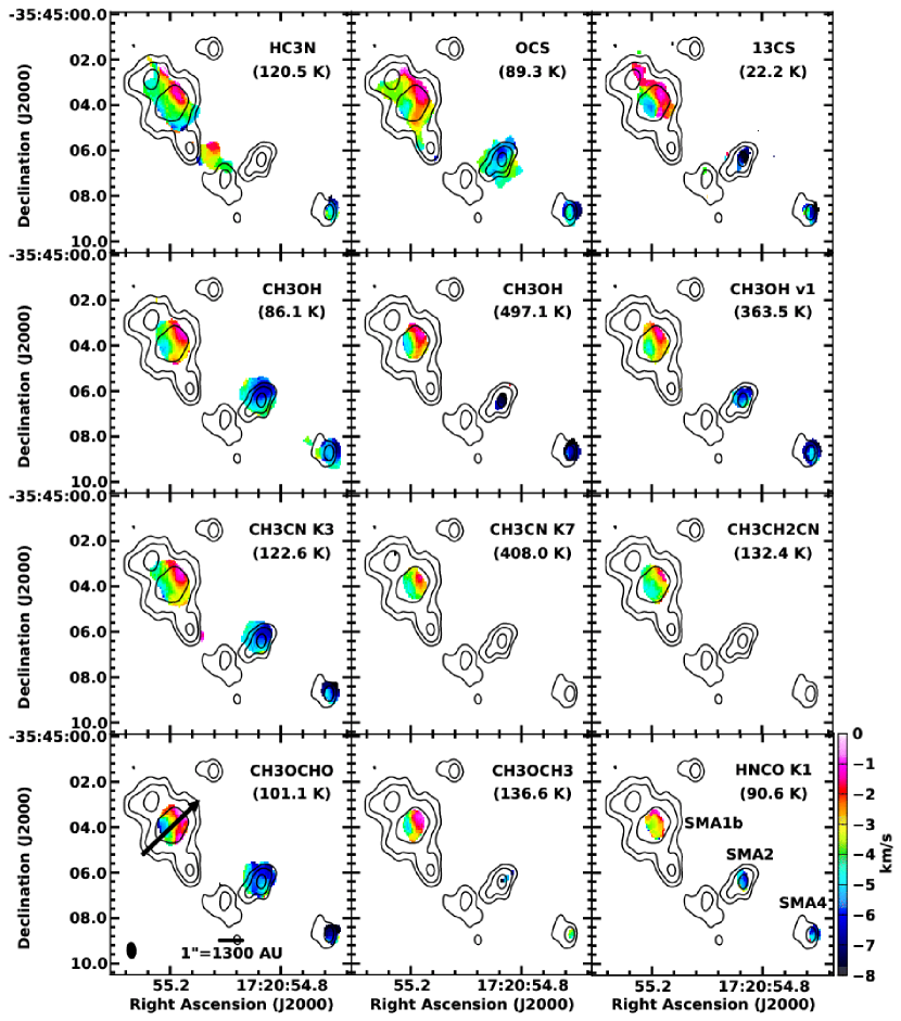
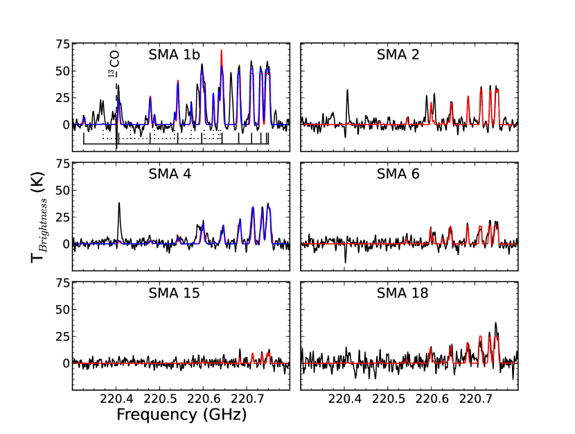
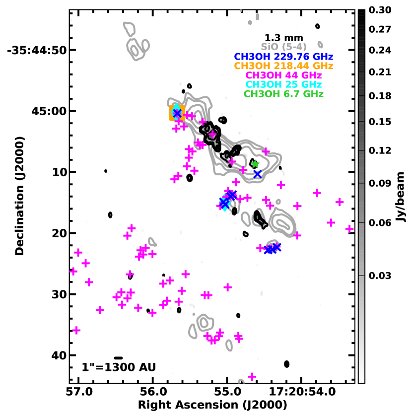
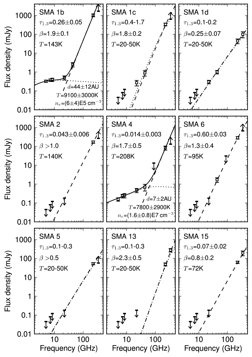
au.clusterStatistics(’25regions_clb_ap_big.crtf.imfit.with_h2o-c4’,1,2, skyCoordinates=True,maxLines=25,horizontalGrid=10, showplot=True,plotwidths=[0.013,0.017],plotfile=’mst’, filledpoints=[0,2,4,12,15,23])

Figure 10: The minimum spanning tree of the protocluster as defined by the 24 detected sources in Table 2 plus the water maser/6 cm source H₂O-C4 from Table 3. The origin is the mean position of all sources. The filled points are the six sources for which we were able to measure the LSR velocity (Table 7). The horizontal dashed lines demarcate the seven 10″-wide strips in which the protostars were counted (from north to south: 1, 2, 6, 9, 3, 3, 1) in order to compute the effective distance to be used in the calculation of the dynamical mass in § 4.3 by the method of Schwarzschild & Bernstein (1955).

Figure 11: Position-velocity diagrams taken along the position angle of the disk ($-52\arcdeg$) for the same molecular transitions shown in Figure 6. The intensity map is the same in all panels (0-0.6 Jy beam^-1). In all panels, the white contour encompasses the region where emission is expected from an edge-on disk at an LSR velocity of $-3.0$ km s^-1 with a central enclosed mass of 10 $M_{\odot}$ undergoing Keplerian rotation and free-fall. In the HC₃N panel, the parameters of the model are $r_{\rm inner}$=200 AU and $r_{\rm outer}$=800 AU, and the black contour shows the model without free-fall. In the HNCO panel, the parameters are $r_{\rm inner}$=400 AU and $r_{\rm outer}$=500 AU, and in the rest of the panels, the parameters are $r_{\rm inner}$=500 AU and $r_{\rm outer}$=800 AU.

References

- Allison & Goodwin (2011) Allison, R. J., & Goodwin, S. P. 2011, MNRAS, 415, 1967
- Allison et al. (2009) Allison, R. J., Goodwin, S. P., Parker, R. J., et al. 2009, MNRAS, 395, 1449
- Andrews et al. (2009) Andrews, S. M., Wilner, D. J., Hughes, A. M., Qi, C., & Dullemond, C. P. 2009, ApJ, 700, 1502
- Anglada et al. (1998) Anglada, G., Villuendas, E., Estalella, R., et al. 1998, AJ, 116, 2953
- Araya et al. (2005) Araya, E., Hofner, P., Kurtz, S., Bronfman, L., and DeDeo, S.: 2005, ApJS, 157, 279
- Astropy Collaboration et al. (2013) Astropy Collaboration, Robitaille, T. P., Tollerud, E. J., et al. 2013, A&A, 558, A33
- Avalos et al. (2006) Avalos, M., Lizano, S., Rodríguez, L. F., Franco-Hernández, R., & Moran, J. M. 2006, ApJ, 641, 406
- Bae et al. (2011) Bae, J.-H., Kim, K.-T., Youn, S.-Y., et al. 2011, ApJS, 196, 21
- Beltrán et al. (2011) Beltrán, M. T., Cesaroni, R., Neri, R., & Codella, C. 2011, A&A, 525, A151
- Benjamin et al. (2003) Benjamin, R. A., Churchwell, E., Babler, B. L., et al. 2003, PASP, 115, 953
- Beuther et al. (2013) Beuther, H., Linz, H., & Henning, T. 2013, A&A, 558, A81
- Beuther et al. (2008) Beuther, H., Walsh, A. J., Thorwirth, S., et al. 2008, A&A, 481, 169
- Beuther et al. (2007a) Beuther, H., Zhang, Q., Bergin, E. A., et al. 2007a, A&A, 468, 1045
- Beuther et al. (2007b) Beuther, H., Walsh, A. J., Thorwirth, S., et al. 2007b, A&A, 466, 989
- Beuther et al. (2005) Beuther, H., Thorwirth, S., Zhang, Q., et al. 2005, ApJ, 627, 834
- Binney & Tremaine (1987) Binney, J., & Tremaine, S. 1987, Princeton, NJ, Princeton University Press, 1987, 747 p.,
- Bonnell & Smith (2011) Bonnell, I. A., & Smith, R. J. 2011, Computational Star Formation, 270, 57
- Bonnell et al. (2003) Bonnell, I. A., Bate, M. R., & Vine, S. G. 2003, MNRAS, 343, 413
- Bonnell & Davies (1998) Bonnell, I. A., & Davies, M. B. 1998, MNRAS, 295, 691
- Brogan et al. (2011) Brogan, C. L., Hunter, T. R., Cyganowski, C. J., et al. 2011, ApJ, 739, L16
- Brogan et al. (2009) Brogan, C. L., Hunter, T. R., Cyganowski, C. J., et al. 2009, ApJ, 707, 1
- Brogan et al. (2008) Brogan, C. L., Hunter, T. R., Indebetouw, R., et al. 2008, Ap&SS, 313, 53
- Brogan et al. (2007) Brogan, C. L., Chandler, C. J., Hunter, T. R., Shirley, Y. L., & Sarma, A. P. 2007, ApJ, 660, L133
- Carey et al. (2009) Carey, S. J., Noriega-Crespo, A., Mizuno, D. R., et al. 2009, PASP, 121, 76
- Carral et al. (2002) Carral, P., Kurtz, S. E., Rodríguez, L. F., et al. 2002, AJ, 123, 2574
- Cartwright & Whitworth (2004) Cartwright, A., & Whitworth, A. P. 2004, MNRAS, 348, 589
- Casella & Berger (2002) Casella, George, & Bergmer, Roger L., 2002, Statistical Inference, 2nd edn., Cengage Learning,
- Cesaroni et al. (2011) Cesaroni, R., Beltrán, M. T., Zhang, Q., Beuther, H., & Fallscheer, C. 2011, A&A, 533, A73
- Cesaroni et al. (2005) Cesaroni, R., Neri, R., Olmi, L., et al. 2005, A&A, 434, 1039
- Cheung et al. (1978) Cheung, L., Frogel, J. A., Hauser, M. G., and Gezari, D. Y.: 1978, ApJ, 226, L149
- Chibueze et al. (2014) Chibueze, J. O., Omodaka, T., Handa, T., et al. 2014, ApJ, 784, 114
- Churchwell et al. (2009) Churchwell, E., Babler, B. L., Meade, M. R., et al. 2009, PASP, 121, 213
- Codella et al. (2004) Codella, C., Lorenzani, A., Gallego, A. T., Cesaroni, R., & Moscadelli, L. 2004, A&A, 417, 615
- Condon et al. (2012) Condon, J. J., Cotton, W. D., Fomalont, E. B., et al. 2012, ApJ, 758, 23
- Cyganowski et al. (2013) Cyganowski, C. J., Koda, J., Rosolowsky, E., et al. 2013, ApJ, 764, 61
- Cyganowski et al. (2012) Cyganowski, C. J., Brogan, C. L., Hunter, T. R., et al. 2012, ApJ, 760, L20
- Cyganowski et al. (2011) Cyganowski, C. J., Brogan, C. L., Hunter, T. R., Churchwell, E., & Zhang, Q. 2011, ApJ, 729, 124
- Cyganowski et al. (2009) Cyganowski, C. J., Brogan, C. L., Hunter, T. R., & Churchwell, E. 2009, ApJ, 702, 1615
- Cyganowski et al. (2007) Cyganowski, C. J., Brogan, C. L., & Hunter, T. R. 2007, AJ, 134, 346
- de Bruijne (1999) de Bruijne, J. H. J. 1999, MNRAS, 310, 585
- De Buizer & Minier (2005) De Buizer, J. M., & Minier, V. 2005, ApJ, 628, L151
- Dzib et al. (2011) Dzib, S., Loinard, L., Rodríguez, L. F., Mioduszewski, A. J., & Torres, R. M. 2011, ApJ, 733, 71
- Feigelson et al. (2009) Feigelson, E. D., Martin, A. L., McNeill, C. J., Broos, P. S., & Garmire, G. P. 2009, AJ, 138, 227
- Fish et al. (2011) Fish, V. L., Muehlbrad, T. C., Pratap, P., et al. 2011, ApJ, 729, 14
- Franco et al. (2000) Franco, J., Kurtz, Hofner, P., et al. 2000, ApJ, 542, L143
- Fukuzawa & Osamura (1997) Fukuzawa, K., & Osamura, Y. 1997, ApJ, 489, 113
- Garay et al. (1996) Garay, G., Ramirez, S., Rodriguez, L. F., Curiel, S., & Torrelles, J. M. 1996, ApJ, 459, 193
- Gezari (1982) Gezari, D. Y.: 1982, ApJ, 259, L29
- Gómez et al. (2013) Gómez, L., Rodríguez, L. F., & Loinard, L. 2013, Rev. Mexicana Astron. Astrofis., 49, 79
- Gordon (1995) Gordon, M. A. 1995, A&A, 301, 853
- Greenhill et al. (2013) Greenhill, L. J., Goddi, C., Chandler, C. J., Matthews, L. D., & Humphreys, E. M. L. 2013, ApJ, 770, L32
- Hernández-Hernández et al. (2014) Hernández-Hernández, V., Zapata, L., Kurtz, S., & Garay, G. 2014, ApJ, 786, 38
- Hillenbrand (1995) Hillenbrand, L. A. 1995, Ph.D. Thesis, Caltech
- Hirota et al. (2014) Hirota, T., Kim, M. K., Kurono, Y., & Honma, M. 2014, ApJ, 782, L28
- Hughes (1988) Hughes, V. A. 1988, ApJ, 333, 788
- Hunter et al. (2013) Hunter, T., Brogan, C., Cyganowski, C., et al. 2013, Protostars and Planets VI, Heidelberg, July 15-20, 2013. Poster #1B034, 34
- Hunter et al. (2008) Hunter, T. R., Brogan, C. L., Indebetouw, R., & Cyganowski, C. J. 2008, ApJ, 680, 1271
- Hunter et al. (2006) Hunter, T. R., Brogan, C. L., Megeath, S. T., Menten, K. M., Beuther, H., and Thorwirth, S.: 2006, ApJ, 649, 888
- Hutawarakorn & Cohen (2005) Hutawarakorn, B., & Cohen, R. J. 2005, MNRAS, 357, 338
- Jiménez-Serra et al. (2012) Jiménez-Serra, I., Zhang, Q., Viti, S., Martín-Pintado, J., & de Wit, W.-J. 2012, ApJ, 753, 34
- Kalinina et al. (2010) Kalinina, N. D., Sobolev, A. M., and Kalenskii, S. V.: 2010, New A, 15, 590
- Keto (2007) Keto, E. 2007, ApJ, 666, 976
- Keto (2003) Keto, E. 2003, ApJ, 599, 1196
- Kirk & Myers (2011) Kirk, H., & Myers, P. C. 2011, ApJ, 727, 64
- Kirk et al. (2007) Kirk, H., Johnstone, D., & Tafalla, M. 2007, ApJ, 668, 1042
- Kirk et al. (2006) Kirk, H., Johnstone, D., & Di Francesco, J. 2006, ApJ, 646, 1009
- Krumholz et al. (2009) Krumholz, M. R., Klein, R. I., McKee, C. F., Offner, S. S. R., & Cunningham, A. J. 2009, Science, 323, 754
- Kuiper et al. (1995) Kuiper, T. B. H., Peters, W. L., III, Forster, J. R., Gardner, F. F., & Whiteoak, J. B. 1995, ApJ, 446, 692
- Kumar & Schmeja (2007) Kumar, M. S. N., & Schmeja, S. 2007, A&A, 471, L33
- Kurtz et al. (2004) Kurtz, S., Hofner, P., & Álvarez, C. V. 2004, ApJS, 155, 149
- Mannings & Sargent (2000) Mannings, V., & Sargent, A. I. 2000, ApJ, 529, 391
- Martín et al. (2012) Martín, S., Martín-Pintado, J., Montero-Castaño, M., Ho, P. T. P., & Blundell, R. 2012, A&A, 539, A29
- Maschberger et al. (2010) Maschberger, T., Clarke, C. J., Bonnell, I. A., & Kroupa, P. 2010, MNRAS, 404, 1061
- McKee & Tan (2003) McKee, C. F., & Tan, J. C. 2003, ApJ, 585, 850
- McMullin et al. (2007) McMullin, J. P., Waters, B., Schiebel, D., Young, W., & Golap, K. 2007, Astronomical Data Analysis Software and Systems XVI, 376, 127
- Megeath & Tieftrunk (1999) Megeath, S. T., & Tieftrunk, A. R. 1999, ApJ, 526, L113
- Meier & Turner (2005) Meier, D. S., & Turner, J. L. 2005, ApJ, 618, 259
- Menten & Batrla (1989) Menten, K. M., & Batrla, W. 1989, ApJ, 341, 839
- Myers et al. (2013) Myers, A. T., McKee, C. F., Cunningham, A. J., Klein, R. I., & Krumholz, M. R. 2013, ApJ, 766, 97
- Milam et al. (2005) Milam, S. N., Savage, C., Brewster, M. A., Ziurys, L. M., & Wyckoff, S. 2005, ApJ, 634, 1126
- Mocanu et al. (2013) Mocanu, L. M., Crawford, T. M., Vieira, J. D., et al. 2013, ApJ, 779, 61
- Natta et al. (2000) Natta, A., Grinin, V., & Mannings, V. 2000, Protostars and Planets IV, 559
- Neckel (1978) Neckel, T. 1978, A&A, 69, 51
- Olnon (1975) Olnon, F. M. 1975, A&A, 39, 217
- Ossenkopf & Henning (1994) Ossenkopf, V., & Henning, T. 1994, A&A, 291, 943
- Osterloh & Beckwith (1995) Osterloh, M., & Beckwith, S. V. W. 1995, ApJ, 439, 288
- Palau et al. (2013) Palau, A., Fuente, A., Girart, J. M., et al. 2013, ApJ, 762, 120
- Pankonin et al. (2001) Pankonin, V., Churchwell, E., Watson, C., and Bieging, J. H.: 2001, ApJ, 558, 194
- Parker et al. (2014) Parker, R. J., Wright, N. J., Goodwin, S. P., & Meyer, M. R. 2014, MNRAS, 438, 620
- Persi and Tapia (2008) Persi, P. and Tapia, M.: 2008, Star Formation in NGC 6334, pp 456–+
- Petrov et al. (2006) Petrov, L., Kovalev, Y. Y., Fomalont, E. B., & Gordon, D. 2006, AJ, 131, 1872
- Pinheiro et al. (2010) Pinheiro, M. C., Copetti, M. V. F., & Oliveira, V. A. 2010, A&A, 521, A26
- Pleuss et al. (2000) Pleuss, P. O., Heller, C. H., & Fricke, K. J. 2000, A&A, 361, 913
- Prim (1957) Prim, R. C. 1957, Bell System Technical Journal, 36, 1389
- Qi et al. (2008) Qi, C., Wilner, D. J., Aikawa, Y., Blake, G. A., & Hogerheijde, M. R. 2008, ApJ, 681, 1396
- Qiu et al. (2012) Qiu, K., Zhang, Q., Beuther, H., & Fallscheer, C. 2012, ApJ, 756, 170
- Rathborne et al. (2010) Rathborne, J. M., Jackson, J. M., Chambers, E. T., et al. 2010, ApJ, 715, 310
- Reid et al. (2014) Reid, M. J., Menten, K. M., Brunthaler, A., et al. 2014, ApJ, 783, 130
- Remijan et al. (2004) Remijan, A., Sutton, E. C., Snyder, L. E., et al. 2004, ApJ, 606, 917
- Reynolds (1986) Reynolds, S. P. 1986, ApJ, 304, 713
- Rodón et al. (2008) Rodón, J. A., Beuther, H., Megeath, S. T., & van der Tak, F. F. S. 2008, A&A, 490, 213
- Rodríguez et al. (2007) Rodríguez, L. F., Zapata, L. A., and Ho, P. T. P.: 2007, ApJ, 654, L143
- Rodríguez et al. (2005) Rodríguez, L. F., Garay, G., Brooks, K. J., & Mardones, D. 2005, ApJ, 626, 953
- Rodríguez et al. (2003) Rodríguez, L. F., Carral, P., Kurtz, S. E., et al. 2003, Revista Mexicana de Astronomia y Astrofisica Conference Series, 15, 194
- Rodriguez & Reipurth (1994) Rodriguez, L. F., & Reipurth, B. 1994, A&A, 281, 882
- Russeil et al. (2010) Russeil, D., Zavagno, A., Motte, F., Schneider, N., Bontemps, S., and Walsh, A. J.: 2010, A&A, 515, A55+
- Sandell (2000) Sandell, G.: 2000, A&A, 358, 242
- Sault et al. (1995) Sault, R. J., Teuben, P. J., & Wright, M. C. H. 1995, Astronomical Data Analysis Software and Systems IV, 77, 433
- Schmeja & Klessen (2006) Schmeja, S., & Klessen, R. S. 2006, A&A, 449, 151
- Schneider et al. (2009) Schneider, P. C., Günther, H. M., & Schmitt, J. H. M. M. 2009, A&A, 508, 321
- Schwarzschild & Bernstein (1955) Schwarzschild, M., & Bernstein, S. 1955, ApJ, 122, 200
- Smith et al. (2009) Smith, R. J., Longmore, S., & Bonnell, I. 2009, MNRAS, 400, 1775
- Straw and Hyland (1989) Straw, S. M. and Hyland, A. R.: 1989, ApJ, 340, 318
- Szymczak et al. (2005) Szymczak, M., Pillai, T., & Menten, K. M. 2005, A&A, 434, 613
- Tan et al. (2014) Tan, J. C., Beltran, M. T., Caselli, P., et al. 2014, arXiv:1402.0919
- Testi et al. (1999) Testi, L., Palla, F., & Natta, A. 1999, A&A, 342, 515
- Thorwirth et al. (2007) Thorwirth, S., Walsh, A. J., Wyrowski, F., et al. 2007, Molecules in Space and Laboratory,
- Thorwirth et al. (2003) Thorwirth, S., Winnewisser, G., Megeath, S. T., and Tieftrunk, A. R.: 2003, in ASP Conf. Ser. 287: Galactic Star Formation Across the Stellar Mass Spectrum, pp 257–260
- Tideswell et al. (2010) Tideswell, D. M., Fuller, G. A., Millar, T. J., & Markwick, A. J. 2010, A&A, 510, A85
- Tobin et al. (2013) Tobin, J. J., Hartmann, L., Chiang, H.-F., et al. 2013, ApJ, 771, 48
- Tofani et al. (1995) Tofani, G., Felli, M., Taylor, G. B., & Hunter, T. R. 1995, A&AS, 112, 299
- Trinidad et al. (2003) Trinidad, M. A., Curiel, S., Cantó, J., et al. 2003, ApJ, 589, 386
- Urquhart et al. (2011) Urquhart, J. S., Morgan, L. K., Figura, C. C., et al. 2011, MNRAS, 418, 1689
- van der Tak et al. (2006) van der Tak, F. F. S., Walmsley, C. M., Herpin, F., & Ceccarelli, C. 2006, A&A, 447, 1011
- Voronkov et al. (2014) Voronkov, M. A., Caswell, J. L., Ellingsen, S. P., Green, J. A., & Breen, S. L. 2014, MNRAS, 439, 2584
- Voronkov et al. (2012) Voronkov, M. A., Caswell, J. L., Ellingsen, S. P., et al. 2012, IAU Symposium, 287, 433
- Walsh et al. (2010) Walsh, A. J., Thorwirth, S., Beuther, H., & Burton, M. G. 2010, MNRAS, 404, 1396
- Walsh et al. (1998) Walsh, A. J., Burton, M. G., Hyland, A. R., & Robinson, G. 1998, MNRAS, 301, 640
- Wang et al. (2012) Wang, K.-S., van der Tak, F. F. S., & Hogerheijde, M. R. 2012, A&A, 543, A22
- Willis et al. (2013) Willis, S., Marengo, M., Allen, L., et al. 2013, ApJ, 778, 96
- Wilson & Coffeen (1954) Wilson, O. C., & Coffeen, M. F. 1954, ApJ, 119, 197
- Xu et al. (2012) Xu, J.-L., Wang, J.-J., & Ning, C.-C. 2012, ApJ, 744, 175
- Zapata et al. (2010) Zapata, L. A., Tang, Y.-W., & Leurini, S. 2010, ApJ, 725, 1091
- Zhang et al. (2007) Zhang, Q., Hunter, T. R., Beuther, H., et al. 2007, ApJ, 658, 1152
- Zinchenko et al. (2012) Zinchenko, I., Liu, S.-Y., Su, Y.-N., et al. 2012, ApJ, 755, 177
- Zinnecker & Yorke (2007) Zinnecker, H., & Yorke, H. W. 2007, ARA&A, 45, 481