Supernova Relic Neutrinos and the Supernova Rate Problem: Analysis of Uncertainties and Detectability of ONeMg and Failed Supernovae

Abstract

Direct measurements of the core-collapse supernova rate ($R_{SN}$) in the redshift range $0\leq z\leq 1$ appear to be about a factor of two smaller than the rate inferred from the measured cosmic massive-star formation rate (SFR). This discrepancy would imply that about one half of the massive stars that have been born in the local observed comoving volume did not explode as luminous supernovae. In this work we explore the possibility that one could clarify the source of this ”supernova rate problem” by detecting the energy spectrum of supernova relic neutrinos with a next generation $10^{6}$ ton water Čerenkov detector like Hyper-Kamiokande. First, we re-examine the supernova rate problem. We make a conservative alternative compilation of the measured SFR data over the redshift range 0 $\leq z\leq$ 7. We show that, by only including published SFR data for which the dust obscuration has been directly determined, the ratio of the observed massive SFR to the observed supernova rate $R_{SN}$ has large uncertainties $\sim 1.8^{+1.6}_{-0.6}$, and is statistically consistent with no supernova rate problem. If we further consider that a significant fraction of massive stars will end their liives as faint ONeMg SNe or as failed SNe leading to a black hole remnant, then the ratio reduces to $\sim 1.1^{+1.0}_{-0.4}$ and the rate problem is essentially solved. We next examine the prospects for detecting this solution to the supernova rate problem. We first study the sources of uncertainty involved in the theoretical estimates of the neutrino detection rate and analyze whether the spectrum of relic neutrinos can be used to independently identify the existence of a supernova rate problem and its source. We consider an ensemble of published and unpublished core collapse supernova simulation models to estimate the uncertainties in the anticipated neutrino luminosities and temperatures. We illustrate how the spectrum of detector events might be used to establish the average neutrino temperature and constrain SN models. We also consider supernova $\nu$-process nucleosynthesis to deduce constraints on the temperature of the various neutrino flavors. We study the effects of neutrino oscillations on the detected neutrino energy spectrum and also show that one might distinguish the equation of state (EoS) as well as the cause of the possible missing luminous supernovae from the detection of supernova relic neutrinos. We also analyze a possible enhanced contribution from failed supernovae leading to a black hole remnant as a solution to the supernova rate problem. We conclude that indeed it might be possible (though difficult) to measure the neutrino temperature, neutrino oscillations, the EOS, and confirm this source of missing luminous supernovae by the detection of the spectrum of relic neutrinos.

1. Introduction

Massive stars ($M\geq 8$ M_⊙) culminate their evolution as core collapse supernovae (CC-SNe). Such supernovae are of particular interest because they are unique sources for all three flavors of energetic neutrinos. An intensive flux of neutrinos with total energy of order $\sim 10^{53}$ ergs is emitted over an interval of $\sim 10$ s during core-collapse supernovae. This energy corresponds to almost 99$\%$ of the released gravitational binding energy during the formation of a 1.4 $M_{\odot}$ proto-neutron star, and this neutrino luminosity is nearly equally partitioned among the three neutrino flavors, i.e. $\nu_{{\rm e},\mu,\tau}$ and their antiparticles. In the case that a black hole is formed instead of a neutron star in the core-collapse of more massive stars, a similar energy $\sim 10^{53}$ ergs is expected to be carried away by more energetic neutrinos during a shorter time interval $\leq 1$ s. If however, a massive star ends its life as an ONeMg supernova, the neutrino flux and energies are diminished. In this paper we investigate the possibility of detecting the various contributions to the supernova relic neutrino background in a $10^{6}$ ton next-generation water Čerenkov detector such as the proposed Hyper-Kamiokande.

Neutrinos are weakly interacting elementary particles, and therefore emerge from deep within the interior of core collapse supernovae. As such, supernova neutrinos have the potential to provide information regarding the physical processes that take place inside the star. For the same reason, the emitted neutrinos can almost freely stream from the time of the early galaxy formation epoch until the present time without absorption in the intervening intergalactic material. Since massive stars have lifetimes ($\sim 10^{6}$ to $10^{7}$ y) that are much shorter than the cosmic age ($\sim 10^{10}$y), supernova neutrinos can be considered to have been emitted almost continuously since the very earliest phase of galaxy formation. This diffuse galactic background of accumulated neutrinos due to SNe is referred to (e.g. Totani et al. (1996) and refs. therein) as the supernova relic neutrinos (SRNs).

The detection of these supernova relic neutrinos and their energy spectrum could be used to study the supernova history from the beginning of galaxy formation (Hopkins & Beacom, 2006). Such data could also provide information on neutrino properties such as flavor oscillations (Chakraborty, Choubey & Kar, 2011; Lunardini & Tamborra, 2012) and/or the neutrino temperatures produced in supernova explosions. One may even be able to discern (Nakazato, 2013) the shock revival time from the detected spectrum of relic neutrinos. Indeed, a next generation Hyper-Kamiokande detector with a mega-ton of pure water is currently being planned with a goal of measuring the relic neutrino background spectrum. Moreover, results from the Super-Kamiokande collaboration (Bayes et al., 2012) already place interesting limits on the total neutrino energies and temperatures from the background spectrum of supernova relic neutrinos (Bayes et al., 2012; Sekiya, 2013).

However, theoretical predictions of the detection rate of supernova relic neutrinos are still subject to a number of uncertainties. These uncertainties include the star formation rate and/or supernova rate and the spectral energy distributions of the three flavors of supernova neutrinos. These in turn depend upon the explosion mechanism, whether the final remnant is a neutron star or black hole, the equation of state (EoS) for proto-neutron stars, and the possibility of neutrino oscillations and self interactions, etc. One goal of the present work is to better clarify these uncertainties.

In this context, it is of particular interest to the present work that an apparent discrepancy has been noted (Horiuchi et al., 2011) between the supernova rate deduced from observations of the cosmic SFR [e.g. Hopkins & Beacom (2006)] at multiple wavelengths, and the detected core-collapse supernova rate ($R_{SN}$) (Leaman et al., 2011; Li et al., 2011a, b; Maoz et al., 2011). The inferred $R_{SN}$ in the redshift range 0 $\leq z\leq$ 1 is about a factor of two smaller than that deduced from the measured SFR. This has been dubbed (Horiuchi et al., 2011) as the ”supernova rate problem.” This discrepancy suggests that either about half of all massive stars are obscured when they explode, or that they do not explode as luminous supernovae.

One explanation for this latter possibility that we explore in this paper is that some of the expected luminous supernovae actually end their lives as faint ONeMg supernovae. Such supernovae should result from progenitor masses in the range 8$M_{\odot}\leq M\leq 10M_{\odot}$ (Isern, Canal & Labay, 1991).

Another aspect is that a significant fraction of relatively massive stars with progenitor masses in the range $M\geq 25$ M_⊙ evolved to failed supernovae leaving black hole remnants rather than to become SNIb,c. In this case, the ejecta falls back onto the central black hole. These failed supernovae have small explosion kinetic energies and are much less luminous. In a series of papers (Lunardini, 2009; Yang & Lunardini, 2011; Keehn & Lunardini, 2012) the contribution of failed SNe to the relic neutrino signal has been analyzed. Here, we expand upon that study by considering the role and associated uncertainties and detectability of failed SNe and also the possibility of an enhanced fraction of such events as a means to resolve the supernova rate problem.

Theoretical studies (Sumiyoshi et al., 2005, 2008; Nakazato et al., 2008) of such failed supernovae, however, show slightly higher neutrino luminosity with much higher neutrino temperatures than those of ordinary supernovae. Depending upon the EoS employed, the difference in neutrino temperatures among the different flavors is even larger than the difference in ordinary supernovae. This opens up the possibility that the spectrum of energetic relic supernova neutrinos could be dominated by a contribution from failed supernovae. A detection of the spectrum of these relic neutrinos could thus provide insight into the supernova rate problem as well as neutrino oscillation effects and the effects of the EoS on supernova collapse (Lunardini & Tamborra, 2012).

One purpose of the present work, therefore, is to explore the possibility that one can solve the ”supernova rate problem” by detecting the energy spectrum of supernova relic neutrinos. For this purpose we first analyze possible uncertainties in both the measured core-collapse supernova rate ($R_{SN}$) and star formation rate (SFR) over the redshift range of 0 $\leq z\leq$ 7. We then study the sources of uncertainty in theoretical calculations of the relic neutrino detection rate.

If we consider only observations for which the dust correction was taken into account, we find that the supernova rate problem has a large uncertainty, i.e. $\sim 1.8^{+1.6}_{-0.6}$ for the ratio of the supernova rate deduced from the observed massive star formation rate (SFR) to the directly observed core-collapse supernova rate $R_{SN}({\rm Obs}$). This is statistically consistent with no supernova rate problem. Moreover, if we consider that a significant fraction of massive stars will end their lives as faint ONeMg SNe or as failed SNe leading to a black hole remnant, then the ratio reduces to $\sim 1.1^{+1.1}_{-0.4}$ and the rate problem is essentially solved.

We next analyze the uncertainties in detecting this solution to the supernova rate problem. We adopt an ensemble of published and unpublished supernova simulation models in order to estimate the uncertainty in the source neutrino luminosities and temperatures. These are taken from core-collapse supernova models leaving either a neutron star or black hole (including possible collapsar gamma-ray burst models) as a remnant, or leading to ONeMg supernovae. We also incorporate several recent studies of supernova nucleosynthesis in order to constrain the neutrino temperatures.

After clarifying and minimizing the temperature uncertainties from the theoretical calculations, we study the effects of different SN models, equations of state, and the effects of the neutrino oscillations on the detected spectrum. We explore whether one can measure the neutrino temperature, distinguish the EoS, and even constrain the unknown neutrino mass hierarchy, through the sensitivity of the resultant detected neutrino spectrum. Finally, we explore whether an enhanced contribution of ”failed supernovae” might be detectable and thereby confirm whether these events are the source of the ”supernova rate problem” (Horiuchi et al., 2011).

2. star formation rate

As noted in the introduction, it is an intriguing conundrum in observational cosmology that the measured core-collapse supernova rate [$R_{SN}({\rm Obs})$] in the redshift range 0$\leq z\leq$1 appears to be about a factor of two smaller than the core-collapse supernova rate deduced from the measured cosmic massive-star formation rate (SFR).

For the present study we consider three different star formation rates as a means to estimate the overall uncertainty in the SFR dependence. For one, we deduce a revised SFR based upon a piecewise linear fit to the observed star formation rate vs. redshift as shown on Figure 1. For illustration we also consider the theoretical SFR model (not shown) of Kobayashi et al. (2000) with and without a correction for dust extinction.

2.1. SFR Data

In view of the importance of clarifying the possible uncertainty in the supernova rate problem we have made an alternative fit to the observed SFR data. As a starting point we use the star formation rate data set employed in Horiuchi et al. (2011). This data set was based upon the compilation of Hopkins & Beacom (2006). A critical part of the SFR data, however, is the correction for extinction by dust. The data of Hopkins & Beacom (2006) is heavily weighted in the interval of $z=0-1$ by the UV data of Balantekin & Yüksel (2005), Wolf et al. (2003) and Arnouts et al. (2005). However, these data were not corrected for obscuration. To implement effective obscurations they utilized the FIR SFR densities (Le Floc’h et al., 2005) up to $z=1$. Although this seems reasonable, the associated dust correction is quite large (up to 80% at $z=1$) and may lead to large systematic errors (Kobayashi et al., 2013). Hence, as an alternative here we consider a more conservative data set that includes only published SFR data for which the dust correction was made by direct observation. This limits our data to a set of 123 data points in X-ray, $\gamma$-ray, UV, Optical, NIR-H$\alpha$, and FIR SFR observations that include dust corrections. In addition to a subset of points from Hopkins & Beacom (2006) these data include some newer data (Reddy & Steidel, 2008; James et al., 2009).

As can be seen on Figure 1, the limitation of the data set to only those that included dust corrections implies a larger uncertainty and lower normalization in the critical redshift range of $z=0-1$ than the compilation of Hopkins & Beacom (2006). This has also been noted in other works (Ouchi et al., 2009; Kobayashi et al., 2013) that discuss the large uncertainties in the dust corrections. Our claim is not that this is a better data set, but that it is a more conservative choice of the data compilation that gives an alternative assessment of the uncertainty in the supernova rate problem.

2.2. fit to the data

For our $\chi^{2}$ fitting, we use the continuous linear [in $\log{(1+z)}$] piecewise star formation rate $\psi_{*}(z)$ as a function of redshift as given in Yüksel et al. (2008), i.e.

$$\psi_{*}(z)=\dot{\rho_{0}}\left[(1+z)^{\alpha\eta}+\left(\frac{1+z}{B}\right)^{\beta\eta}+\left(\frac{1+z}{C}\right)^{\gamma\eta}\right]^{\frac{1}{\eta}},$$ (1)

where our deduced parameters for the best fit and $\pm 1\sigma$ upper and lower limits are given in Table 1 . When deducing the $\pm 1\sigma$ errors in the fit, we use the best-fit value of $\alpha=4.22$. This keeps the curves parallel at low redshift ($z=0-1$) and is consistent with the dispersion in the data. By keeping the curves parallel, the determination of the standard deviation in the fits is just given by a change of normalization to give $\Delta\chi^{2}=1$. The CC-SN rate evolution is assumed to follow the same $(1+z)^{\alpha}$ behavior where $\alpha$ is fixed to 4.22 obtained from SFR fits. This makes a comparison of the overall normalization possible.

In Eq. (1), we have chosen a value of the smoothing parameter $\eta=-10$ consistent with that used in previous works [cf. Hopkins & Beacom (2006); Yüksel et al. (2008); Horiuchi et al. (2011)]. The best fit corresponds to $\chi^{2}=272$ for 118 degrees of freedom implying a reduced $\chi_{r}^{2}=2.3$. Because our adopted data set has a larger dispersion, our $\chi^{2}$ is larger than the fits of Hopkins & Beacom (2006), Yüksel et al. (2008), and Horiuchi et al. (2011). In addition, the data at low redshift cause the best fit slope to be somewhat steeper than in previous works, i.e. $\alpha=4.2$ vs. $\alpha=3.4$ in Hopkins & Beacom (2006), Yüksel et al. (2008) andHoriuchi et al. (2011). This larger value for $\alpha$ also implies that the absolute fit to the SFR at $z=0$ is lower, i.e. we deduce $\dot{\rho}_{0}=0.010^{+0.01}_{-0.004}$ M_⊙ y^-1 (see Table 1) vs. $\dot{\rho}_{0}=0.017$ M_⊙ y^-1 in Horiuchi et al. (2011). This slope, however, also reduces the observed supernova rate so that the supernova rate problem remains at about the same factor as noted below.

We also note that we have not included a correction for the flux sensitivity at high redshift as pointed out in Kistler et al. (2009). Hence, one should not take our fit seriously in the redshift range $z>4$. As noted below, the SFR at high redshift contributes negligibly to the observed SRN spectrum. Thus, for this paper, we are almost entirely concerned with the SFR at low redshift where this correction is not necessary.

Figure 1 shows the data-points from rest-frame X-ray, $\gamma$-ray, UV, Optical, NIR-H$\alpha$, FIR to sub-mm observations compared with our deduced SFR $\psi_{*}$(z) and that given in Yüksel et al. (2008). The thick line shows the best fit SFR. The thin lines show the $\pm 1\sigma$ upper and lower limits to the SFR. As noted above a key difference between our star formation rate data and that of Yüksel et al. (2008) is the limitation to data with published extinction corrections.

As an illustration of the systematic error due the dust extinction corrections, in our analysis below we also consider the theoretical star formation rate deduced in Kobayashi et al. (2000) from a fit to a limited data set both with and without dust corrections. As shown in that paper, the magnitude of the dust correction is comparable to the error bars in the piecewise linear star formation rate of Figure 1.

On the other hand, as shown below, there is little difference between the relic neutrino detection rate with either form for the SFR. For our purposes we will mainly utilize the piecewise linear SFR as the best direct representation of the observed massive star formation rate. However, for illustration, we also make some comparisons with the rate of Kobayashi et al. (2000) with and without dust correction.

2.3. Core-Collapse Supernova Rate

To deduce the core-collapse supernova rate from the total SFR one must determine the fraction of total stars that produce observable supernovae. In the estimated visible supernova rate of Horiuchi et al. (2011) it was assumed that all massive progenitors from 8 to 40 M_⊙ lead to visible SNe. The higher end of this mass range corresponds to SNIb,c, while the lower end corresponds to normal SNII.

We similarly include contributions from both normal core-collapse SNII and SNIb,c, the latter of which accounts for about $\sim 25\pm 10$% of observed core-collapse supernova rate at redshift near $z=0$ (Smartt, 2009). However, we treat the possibility of failed SNe forming a black hole and dim NeOMg supernovae in the low mass end. Hence, for the total observed core-collapse SN rate we write:

$$R_{SN}(z)=R_{SNII}(z)+R_{SNIb,c}(z)$$ (2)

The mass range for Type-II supernova progenitor stars is taken to be from 8 to 25 M_⊙. The minimum mass for observed CC-SN progenitors appears to be $\approx 8\pm 1$ M_⊙ (Smartt, 2009). Nevertheless, there is large uncertainty in the degree to which progenitors have experienced mass loss and the true initial progenitor mass could be greater. Moreover, it is believed (Heger et al., 2003) that initial progenitor stars in the mass range of 8-10 M_⊙ collapse as an electron degenerate ONeMg core and do not produce bright supernovae. Hence, we also consider a lower limit of 10 M_⊙ as discussed below when allowing for the possibility of ONeMg SNe.

Regarding SNIb,c, although it is known (Smartt, 2009) that they are associated with massive star forming regions, there is some ambiguity as to their progenitors. There are two theoretical possibilities. Heger et al. (2003) and Fryer, Woosley & Hartmann (1999) have studied the possibility that massive stars ($M\sim 25-100$ M_⊙) can shed their outer envelope by radiative driven winds leading to bright SNIb,c supernovae. This source for SNIb,c was adopted in Horiuchi et al. (2011) by assuming that all stars with ($M\sim(25-40)$ M_⊙) explode as SNIb,c. We also adopt this as one possibility. We note that Hopkins & Beacom (2006) adopted a range of (25-50) M_⊙ for SNIb,c. Changing the upper mass limit from 40 50 M_⊙ to 50 M_⊙ makes only a slight difference ( 1%) in the inferred total core-collapse supernova rate.

Theoretically, however, this single massive-star paradigm does not occur as visible SNIb,c supernovae until well above solar metallicity (Heger et al., 2003). At lower metallicity most massive stars with $M>25$ M_⊙ collapse as failed supernovae with black hole remnants. Hence, this mechanism is not likely to contribute to the observed SNIb,c rate at the higher redshifts of interest here. On the other hand, it has been estimated (Fryer, Woosley & Hartmann, 1999) that 15 to 30% of massive stars up to $\sim 40$ M_⊙ are members of interacting binaries that can shed their outer envelopes by roche-lobe overflow (Podsiadlowski et al., 1992; Nomoto et al., 1995) leading to bright SNIb,c supernovae. We also consider that hypothesis here. To do so we take a fraction $f_{b}$ of all massive stars in the range of (8 to 40) M_⊙ to result in bright SNIb,c via binary interaction. We adopt $f_{b}=0.25$ consistent with the observed SNIb,c rate (Smartt, 2009) and the theoretical estimate of Fryer, Woosley & Hartmann (1999).

Hence, for $R_{SNIb,c}(z)$ we write two possibilities. One is:

$$\begin{array}[]{c}R^{s}_{SNIb,c}(z)=\psi_{*}(z)\times\frac{\int_{25M_{\sun}}^{40M_{\sun}}dM\phi(M)}{\int_{M_{min}}^{M_{max}}dMM\phi(M)}~{}~{},\end{array}$$ (3)

where the superscript $s$ denotes the single-star paradigm. The other possibility is

$$\begin{array}[]{c}R^{b}_{SNIb,c}(z)=f_{b}\psi_{*}(z)\times\frac{\int_{8M_{\sun}}^{40M_{\sun}}dM\phi(M)}{\int_{M_{min}}^{M_{max}}dMM\phi(M)}~{}~{},\end{array}$$ (4)

where superscript $b$ denotes the interacting binary paradigm.

Similarly, then the rate of normal core-collapse SNII, $R_{SNII}(z)$, is given by

$$\begin{array}[]{c}R_{SNII}(z)=(1-f_{b})\psi_{*}(z)\times\frac{\int_{8M_{\sun}}^{25M_{\sun}}dM\phi(M)}{\int_{M_{min}}^{M_{max}}dMM\phi(M)}~{}~{},\end{array}$$ (5)

where the case of the interacting binary SNIb,c scenario, $R_{SNII}(z)$ is reduced to allow a fraction $f_{b}$ of stars to be in interacting binaries.

As in Horiuchi et al. (2011) we adopt the modified broken power-law Salpeter A IMF (Baldry & Glazebrook, 2003),

$$\phi(M)=M^{-\zeta}~{}~{},$$ (6)

with $\zeta=2.35$ for stars with $M\geq 0.5$ M_⊙ and $\zeta=1.5$ for $0.1$ M${}_{\odot}<M<0.5$ M_⊙. The star formation rate $\psi_{*}(z)$ is taken to be the piecewise linear rate shown in Figure 1. For the integration normalization we adopt M${}_{min}=0.1$ M_⊙ and M${}_{max}=125$ M_⊙. We note that Hopkins & Beacom (2006) and Horiuchi et al. (2011) adopted M${}_{max}=100$ M_⊙, while a number of authors [e.g. Ando (2004); Lunardini (2009); Lunardini & Tamborra (2012)] use 125 M_⊙ based upon the models of Heger et al. (2003). Nevertheless, as noted in Hopkins & Beacom (2006), there is almost no contribution from stars above 100 M_⊙ and there is no significant difference ($\sim 1$%) between the use of 125 or 100 M_⊙ as the upper limit. Hence, there is no need to correct the data for whether the observers employed 100 or 125 M_⊙ in the upper limit of the IMF used to deduce the SFR.

2.4. Failed Supernovae

For failed supernovae (fSNe) we consider all single massive stars with progenitor masses with $M>25$ M_⊙, (Heger et al., 2003), although this cutoff is uncertain. For stars above this cutoff mass the whole star collapses leading to a black hole and no detectable supernovae. Allowing for 25% of stars with $M=(25-40)$ M_⊙ to form SNIb,c by binary interaction as noted above, then the rate for failed supernovae is given by,

$$R({\rm fSN}) = (1-f_{b})\psi_{*}(z)\times\frac{\int_{25M_{\sun}}^{40M_{\sun}}dM\phi(M)}{\int_{M_{min}}^{M_{max}}dMM\phi(M)}~{}~{}$$ (7)

$$+\psi_{*}(z)\times\frac{\int_{40M_{\sun}}^{125M_{\sun}}dM\phi(M)}{\int_{M_{min}}^{M_{max}}dMM\phi(M)}~{}~{}.$$

2.5. ONeMg Supernovae

We also consider here the possibility of ONeMg (or electron-capture) supernovae. Such stars involve explosion energies and luminosities that are an order of magnitude less than normal core collapse supernovae. Hence, they may go undetected. ONeMg supernovae are believed to arise from progenitor masses in the range of 8 $M_{\odot}\leq M\leq 10M_{\odot}$. Such supernovae occur (Isern, Canal & Labay, 1991) when an electron-degenerate ONeMg core reaches a critical density (at $M_{core}\sim 1.4$ M_⊙). In this case the electron Fermi energy exceeds the threshold for electron capture on ²⁴Mg. These electron captures cause a loss of hydrostatic support from the electrons and also a heating of the material. Ultimately, this leads to a dynamical collapse and the ignition of an O-Ne-Mg burning front that consumes the star. The rate for ONeMg SNe is then taken to be,

$$\begin{array}[]{c}R({\rm ONeMg~{}SN})=(1-f_{b})\psi_{*}(z)\times\frac{\int_{8M_{\sun}}^{10M_{\sun}}dM\phi(M)}{\int_{M_{min}}^{M_{max}}dMM\phi(M)}~{}~{},\end{array}$$ (8)

where the integration limits in the denominator are the same as for $R_{S}N$ as given below Eq. (5), and the factor of $(1-f_{b})=0.75$ arises in the binary SNIb,c paradigm. In this case, the lower limit for the progenitors of SNII and SNIb,c becomes 10 M_⊙ instead of 8 M_⊙.

With our adopted integration limits and IMF parameters, the reduction factor from the SFR to the deduced supernova rate is $R_{SN}({\rm calc})/SFR=0.010$ for the single-star SNIb,c paradigm. The factor reduces to 0.0093 if failed supernovae are removed for $M>25$ M_⊙ in the interacting binary scenario, and if faint ONeMg supernovae are undetected for stars with $8$ M_⊙ $<M<10$ M_⊙, the factor reduces to 0.0063.

2.6. Supernova Rate Problem

To analyze the supernova rate problem, one must compare the above scenarios for visible core-collapse supernovae with the rate of those observationally detected. As in Horiuchi et al. (2011) we fit the seven measured core collapse supernova rates $R_{SN}({\rm Obs})$ in the redshift range of $z=0-1$ deduced in Li et al. (2011b), Cappellaro et al. (1999), Botticella et al. (2008), Cappellaro et al. (2005), Bazin et al. (2009) and Dahlen, et al. (2004) as given in Table 1 of Horiuchi et al. (2011). Also, as in Horiuchi et al. (2011) we use the functional form

$$R_{SN}({\rm Obs})=a(1+z)^{b}~{}~{}.$$ (9)

However, we find a much better fit for $b=4.22$ ($\chi^{2}=1.8$) from our fit to the SFR rather than $b=3.4$ ($\chi^{2}=2.5$) as in Horiuchi et al. (2011). With $b=4.22$, the best fit normalization is for $a=0.60\pm 0.07$.

With this observed core collapse SN rate we obtain the following characterizations of the supernova rate problem.

$$\frac{R_{SN}({\rm calc})}{R_{SN}({\rm obs})} = 1.8^{+1.6}_{-0.6}~{}~{}~{}{\rm single~{}star~{}SNIb,c}~{},$$ (10)

$$= 1.6^{+1.5}_{-0.6}~{}~{}~{}{\rm binary~{}SNIb,c+fSNe}~{},$$ (11)

$$= 1.1^{+1.0}_{-0.4}~{}~{}~{}{\rm binary~{}SNIb,c+fSNe}$$ (12)

$${\rm+~{}ONeMg~{}SNe}~{}.$$

If we adopt the likely possibility that failed black-hole producing supernovae and faint ONeMg supernovae account for the unobserved supernovae, then there is essentially no supernova rate problem. Indeed, with our inferred uncertainties, all three possibilities are consistent with no supernova rate problem at the $1\sigma$ level as also noted in Kobayashi et al. (2013).

On the other hand, as much as a factor of 2 discrepancy as deduced in Horiuchi et al. (2011) is not ruled out. The reason for the difference between the ratio deduced here and that in Horiuchi et al. (2011) is that we have only included data with published corrections for dust obscuration. One can see from the dotted line in Figure 1 that the SFR of Hopkins & Beacom (2006), Yüksel et al. (2008) andHoriuchi et al. (2011) is systematically higher in the redshift intervals $z=0-1$ and $4-7$. The discrepancy at high redshift is not particularly relevant to the present work. The star formation rate at high redshift requires a correction (Kistler et al., 2009) for unseen galaxies and is probably best deduced from GRBs at high redshift. The main focus of this study, however, is the SFR in the interval $z=0-1$.

In what follows we will examine whether this solution to the supernova rate problem can be determined observationally. A key point is that, although black-hole forming and ONeMg SNe are optically dim, they are quite luminous in neutrinos. Hence, as a means to test this hypothesis we analyze whether the relic neutrino detection rate and spectrum can be used to identify one or the other possible solutions to the putative supernova rate problem. To do that we next analyze the relic neutrino background, the detector response, and the associated uncertainties.

3. SRN background

In this section we analyze the detection rate and spectrum along with various theoretical uncertainties in the predicted SRN background. As a fiducial detector, we consider a Hyper-Kamiokande next-generation Čerenkov detector. This detector is proposed (Abe et al., 2003) to consist of a mega-ton of pure water laden with 0.2$\%$ GdCl₃ to reduce the background (Beacom & Vagins, 2004). Our goal is to clarify the uncertainties involved in estimates of the detection rate.

Most of the uncertainties arise from the energy flux of the arriving SRNs. The presently observed SRN flux spectrum ${dN_{\nu}}/{dE_{\nu}}$ can be derived (Strigari et al., 2005; Yüksel & Beacom, 2007) from an integral over the cosmic redshift $z$, of the neutrinos emitted per supernova and the cosmic supernova rate per unit redshift $R_{SN}(z)$:

$$\frac{dN_{\nu}}{dE_{\nu}} = \frac{c}{H_{0}}\int_{0}^{z_{max}}R_{SN}(z)\frac{dN_{\nu}(E^{\prime}_{\nu})}{dE^{\prime}_{\nu}}$$ (13)

$$\times \frac{dz}{\sqrt{\Omega_{m}(1+z)^{3}+\Omega_{\Lambda}}}~{}~{},$$

where $z_{max}$ is the redshift at which star formation begins. For our purposes we take $z_{max}=5$. $R_{SN}$ is the number of supernovae per unit redshift per comoving volume as discussed in the previous section. The quantity $dN_{\nu}(E^{\prime}_{\nu})/dE^{\prime}_{\nu}$ is the emitted neutrino spectrum at the source, where the energy $E^{\prime}_{\nu}=(1+z)E_{\nu}$ is the energy at emission, while $E_{\nu}$ is the redshifted energy observed in the detector. In the present work we improve upon previous estimates based only upon the neutrino emission from a typical type II core collapse supernovae. As described below, we also average over the neutrino emission from ONeMg electron-capture supernovae and the truncated neutrino emission from the collapse of massive stars to form black holes in addition to averaging over the range of progenitor models for normal Type II supernovae.

Here and throughout we assume a standard $\Lambda$CDM cosmology. The quantities $\Omega_{m}$ and $\Omega_{\Lambda}$ are the contributions to the closure density of total baryonic plus dark matter and the cosmological dark energy, respectively. In this work, we adopt a standard $H_{0}=70$ km s^-1 Mpc^-1, $\Omega_{m}=0.3,~{}\Omega_{\Lambda}=0.7$ cosmology [as in Horiuchi et al. (2011)]. This is consistent with the best-fit WMAP9 parameters (Hinshaw et al., 2013), i.e. $H_{0}=68.92^{+0.94}_{-0.95},~{}\Omega_{m}=0.2855^{+0.0096}_{-0.0097}$ and $\Omega_{\Lambda}=0.717\pm 0.011$.

In this study, we calculate SRN detection rate for a water Čerenkov detector with a fiducial volume of 1.0 $\times$ 10⁶ ton (laden with 0.2$\%$ GdCl₃). As shown below, the threshold energy for SRN detection is $\sim 10$ MeV due to the existence of background $\bar{\nu_{e}}$ emitted from terrestrial nuclear reactors, while the upper detection limit is $\sim 33$ to 37 MeV due to the existence of the atmospheric $\bar{\nu_{e}}$ background. The SRN energy spectrum at detection can then be written as:

$$\frac{dN_{event}}{dE_{e^{+}}}=N_{target}\cdot\varepsilon(E_{\nu})\cdot\frac{1}{c}\cdot\frac{dF_{\nu}}{dE_{\nu}}\cdot\sigma(E_{\nu})\cdot\frac{dE_{\nu}}{dE_{e^{+}}}$$ (14)

where $N_{target}$ is the number of target particles in the water Čerenkov detector, $\varepsilon(E_{\nu})$ is the efficiency for neutrino detection, ${dF_{\nu}}/{dE_{\nu}}$ is the incident flux of SRNs, and $\sigma(E_{\nu})$ is the cross section for neutrino absorption: $\bar{\nu_{e}}+p\to e^{+}+n$, and $E_{\nu}=E_{e^{+}}+1.3~{}{\rm MeV}$. For simplicity we set $\varepsilon(E_{\nu})$ = 1.0, and we use the cross sections given in Strumia & Vissani (2003) when calculating the reaction rate of SRN with target particles in the detector.

We only consider the detection of $\bar{\nu_{e}}$, because the cross section in a water Čerenkov detector for the $\bar{\nu_{e}}+p\to e^{+}+n$ reaction is about 10² times larger than that for $\nu_{e}$ detection via $\nu_{e}+n\to e^{-}+p$.

4. Neutrino spectra from Core Collapse SNe

Next, we analyze the uncertainties in the emitted neutrino spectrum, i.e. ${dN_{\nu}(E^{\prime}_{\nu})}/{dE^{\prime}_{\nu}}$ in Eq. (13).

4.1. Neutrino spectrum for CC-SNe

Although the neutrino temperature T_ν in core collapse SNe may also depend upon progenitor mass (Lunardini & Tamborra, 2012), we note that the dependence on progenitor mass is rather small compared to the uncertainty in the neutrino temperatures themselves. The reason for this is that the mass of most observed neutron stars is rather tightly constrained to be $\sim 1.4$ M_☉ (with a maximum mass of $\sim 2-3$ M_☉). Because the mass is also proportional to the degeneracy pressure, the narrow range of observed remnant neutron star masses suggests that the associated neutrino temperatures should also be tightly constrained. Hence, for our purposes we ignore the dependence on progenitor mass. In this study, therefore, we adopt a fiducial SN 1987A model [i.e. progenitor mass $\simeq$ 16.2 M_☉, remnant mass $\simeq$ 1.4M_☉, liberated binding energy $\simeq$ 3.0 $\times$ 10⁵³ erg (Arnett et al., 1989)]. We assume that this model is representative of every core-collapse SN with progenitor masses in the range of 8 to 25 M_☉ and also every SNIb,c over the adopted mass range for 8-40 M_⊙ in any of the possible paradigms. Furthermore, we assume that the proto-neutron star formed during all core-collapse SN explosions is in thermodynamic equilibrium. Hence, the liberated binding energy is equally divided among the 6 neutrino species (3 flavors and their anti-particles). Even in the context of this single progenitor model, however, there is a range of predicted neutrino temperatures and chemical potentials in various supernova core-collapse simulations in the literature. We now survey them as a means to estimate the uncertainty in the neutrino detection rate due to these parameters.

4.2. Constraint on T${}_{\nu_{e}}$ T${}_{\bar{\nu_{e}}}$, T${}_{\nu_{\mu}}$, T${}_{\nu_{\tau}}$

As discussed below, the uncertainty in the neutrino temperatures constitutes the largest present uncertainty in the expected relic neutrino detection rate. Indeed, recent results from Super-Kamiokande (Bayes et al., 2012; Sekiya, 2013) already place some constraints on the relic neutrino temperatures. In this section we summarize the independent constraints and their uncertainties on theoretical models for the temperatures of emitted neutrinos. One result we make use of is from Yoshida et al. (2008) where it was concluded that the temperature (T${}_{\nu_{x}}$) of $\nu_{\mu}$, $\nu_{\tau}$ and their anti-neutrinos should be in the range 4.3 to 6.5 MeV for SN 1987A models. This constraint is based (Yoshii et al., 1997) upon the observed solar-system meteoritic abundance ratio of boron isotopes. Similarly, it has been demonstrated (Hayakawa et al., 2010) that both T${}_{\nu_{e}}$ and T${}_{\bar{\nu_{e}}}$ should be $\sim 4.0$ MeV to produce the correct abundance ratio of ¹⁸⁰Ta/¹³⁸La.

The range of uncertainty in all neutrino types from core collapse models is indicated in Figures 3a and 3b along with Tables 2-4. The tables summarize values derived in previous models for T${}_{\nu_{e}}$, T${}_{\bar{\nu_{e}}}$, and T${}_{\nu_{x}}$, the dimensionless chemical potentials $\eta_{\nu_{i}}$, and whether the temperatures are derived from the average $<e>$, or the RMS energy $<e^{2}>^{1/2}$. Results are shown from both original published numerical simulations (filled circles in the figures) as summarized in Tables 2-4, and unpublished private communications (empty circles). When the chemical potentials at the neutrino sphere were not apparent in the simulations we assumed a small chemical potential and deduced temperatures from the approximation $T_{i}\approx\langle e\rangle/3.15$. From these data we have adopted the best central temperature values and the $\pm$ 1$\sigma$ uncertainty based upon the $\chi^{2}$ distribution of these data. This is denoted by the orange ellipses in Figures 3a and 3b.

Figure 3a shows the projected correlation between T${}_{\bar{\nu_{e}}}$ and T${}_{\nu_{e}}$ for various supernova simulations, while Figure 3b shows the correlation between T${}_{\nu_{x}}$ and T${}_{\bar{\nu_{e}}}$. Red crosses represent T${}_{\nu_{x}}$ and T${}_{\bar{\nu_{e}}}$ summarized in the Tables 2-4 with assumed errors of $\pm 10\%$ as deduced below.

The neutrino temperature hierarchy requires that T${}_{\nu_{x}}$ $\geq$ T${}_{\bar{\nu_{e}}}$, while the constraint of Yoshida et al. (2008) requires T${}_{\nu_{x}}\sim 4.3$ to 6.5 MeV. We therefore adopt T${}_{\bar{\nu_{e}}}\sim$3.8 to 6.0 MeV as shown by the horizontal lines in Figure 3a and the vertical lines and light blue trapezoid in Figure 3b. We then deduce our adopted constraints on values for the T${}_{\bar{\nu_{e}}}$-T${}_{\nu_{x}}$ correlation as the overlapping area of the orange ellipses and the blue trapezoids as shown in Figure 3b.

We selected seven pairs of T${}_{\bar{\nu_{e}}}$-T${}_{\nu_{x}}$ to use for analyzing the dependence of the SRN energy spectra on T${}_{\bar{\nu_{e}}}$-T${}_{\nu_{x}}$. These are indicated by the green, red, magenta, blue, yellow and two black circles without error bars shown in Figure 3b. These correspond to temperatures (T${}_{\bar{\nu_{e}}}$, T${}_{\nu_{x}}$) = (6.0 MeV, 6.5MeV), (5.0 MeV, 6.0 MeV), (4.1MeV, 6.5MeV), (3.9MeV, 5.6MeV), (4.5MeV, 4.7MeV), (6.7MeV, 7.6MeV) and (2.5MeV, 2.5MeV), respectively. Note that our adopted temperature range is consistent with the 90% C.L. temperatures recently deduced by the Super-Kamiokande collaboration (Bayes et al., 2012; Sekiya, 2013).

The error bars for the points shown on Figures 3a and 3b correspond to the uncertainty due to the variation of the neutrino temperatures in time during the explosion. An analysis was made in Totani et al. (1998) of the time dependence of the supernova neutrino temperature based upon the SN explosion model of Mayle et al. (1987) and assuming a Fremi-Dirac neutrino spectrum. In that work it was concluded that after about 1 sec the neutrino temperatures only vary by about 10% over the next few seconds when most of the neutrino luminosity is emitted. On the other hand, some of the most recent neutrino transport calculations based upon modern relativistic solutions to the Boltzmann Eq. [e.g. Fischer et al. (2012); Roberts (2012)] imply smaller average neutrino temperatures and a more rapid decline of temperature with time. Nevertheless, for our purposes we can adopt a 10% as a reasonable uncertainty due to the decline of the neutrino temperatures with time in Figures 3a and 3b keeping in mind that the true neutrino flux should be derived from a numerical integration of the emitted neutrino flux from the numerical models and may not be perfectly represented by a Fermi-Dirac temperature.

We also note that the time dependence of the correlation between T${}_{\nu_{x}}$ and T${}_{\bar{\nu_{e}}}$ was analyzed in Mayle et al. (1987). That work confirms that our adopted upper and lower limits of T${}_{\nu_{e}}$, T${}_{\bar{\nu_{e}}}$ and T${}_{\nu_{x}}$ are satisfied throughout most of the explosion.

Tables 2 to 4 show the calculated neutrino temperatures and dimensionless chemical potentials $\eta_{\nu}\equiv\mu_{\nu}/T_{\nu}$ from various numerical simulations of core-collapse SN explosions. These data show that there is no universal agreement as to the chemical potential for the emitted supernova neutrinos.

Nevertheless, in spite of this uncertainty, it has been demonstrated [e.g. Yoshida et al. (2005)] that the uncertainty in the reaction rate for any neutrino processes due to the neutrino chemical potential is less than 10% as long as the dimensionless chemical potential $\eta_{\nu}\equiv\mu_{\nu}/T\leq 3.0$. Since this condition is satisfied in Tables 2 to 4, we are justified in ignoring the neutrino chemical potential in the present study, while keeping in mind that this can add to the overall uncertainty in the detection rate.

4.3. Dependence of the SRN energy spectra on Neutrino Oscillations

It is by now well established that the flavor eigenstates for the neutrino are not identical to the mass eigenstates. The flavor eigenstates $\nu_{e}$, $\nu_{\mu}$, $\nu_{\tau}$ are related to the mass eigenstates by an unitary matrix $U$:

$$\left(\begin{array}[]{c}\nu_{e}\\ \nu_{\mu}\\ \nu_{\tau}\end{array}\right)=U\left(\begin{array}[]{c}\nu_{1}\\ \nu_{2}\\ \nu_{3}\end{array}\right)~{}~{},$$ (15)

where the matrix U can be decomposed as:

$$U=\left(\begin{array}[]{ccc}U_{e1}&U_{e2}&U_{e3}\\ U_{\mu 1}&U_{\mu 2}&U_{\mu 3}\\ U_{\tau 1}&U_{\tau 2}&U_{\tau 3}\end{array}\right)$$ (16)

$$\equiv \left(\begin{array}[]{ccc}1&0&0\\ 0&c_{23}&s_{23}\\ 0&-s_{23}&c_{23}\end{array}\right)\left(\begin{array}[]{ccc}c_{13}&0&~{}s_{13}e^{-i\delta}\\ 0&1&0\\ -s_{13}e^{i\delta}&0&c_{13}\end{array}\right)$$ (27)

$$\times\left(\begin{array}[]{ccc}c_{12}&s_{12}&0\\ -s_{12}&c_{12}&0\\ 0&0&1\end{array}\right)~{}~{}.$$

Here, s_ij $\equiv$ $\sin\theta_{ij}$, c_ij $\equiv$ $\cos\theta_{ij}$, and $\theta_{ij}$ is the mixing angle between neutrinos with mass eigenstates i and j, and $\delta$ represents the CP phase.

For the mixing of mass eigenstates one must consider both the normal mass hierarchy, $m_{1}<m_{2}<m_{3}$, and the inverted mass hierarchy, $m_{3}<m_{1}<m_{2}$. Both models have two resonance mass regions. The resonance at higher density is called the H-resonance, and the one at lower density is called the L-resonance. In the normal mass hierarchy, both resonance points are in the neutrino sector. In the inverted mass hierarchy, however, one resonance is in the neutrino sector and the other is in the anti-neutrino sector.

The prospects for detecting effects of neutrino flavor oscillations in the spectrum of detected SRNs has been discussed in Chakraborty, Choubey & Kar (2011) using a parameterized form for the emitted neutrino spectrum from Keil et al. (2003), and also in Lunardini & Tamborra (2012) using the supernova simulations of the Basel group (Fischer et al., 2010). In this study, we similarly consider the possible influence and detectability of neutrino oscillations. Rather than to adopt a particular mixing scenario we explore mixing in the limit of 3 neutrino oscillation paradigms according to Dighe & Smirnov (2000). These are: Case I - normal mass hierarchy case or an inverted mass hierarchy with complete non-adiabatic mixing; Case II - an inverted mass hierarchy case with complete adiabatic mixing; and Case III - no mixing. We also explore the possible effects of a neutrino self interaction below in §4.8.

Let us consider the inverted hierarchy first. If we assume an efficient conversion probability $P_{H}$ of $\bar{\nu}_{3}\leftrightarrow\bar{\nu}_{1}$ at the H-resonance, then the $\bar{\nu}_{e}$ flux emitted from the supernova becomes:

$$\phi_{\bar{\nu}_{e}} = |U_{e1}|^{2}\phi_{\bar{\nu}_{1}}+|U_{e2}|^{2}\phi_{\bar{\nu}_{2}}+|U_{e3}|^{2}\phi_{\bar{\nu}_{3}}$$

$$= |U_{e1}|^{2}\{(1-P_{H})\phi_{\bar{\nu}_{1}}(0)+P_{H}\phi_{\bar{\nu}_{3}}(0)\}$$

$$+ |U_{e2}|^{2}\phi_{\bar{\nu}_{2}}(0)+|U_{e3}|^{2}\{P_{H}\phi_{\bar{\nu}_{1}}(0)+(1-P_{H})\phi_{\bar{\nu}_{3}}(0)\}~{}.$$

From this, one can deduce the survival probability $\bar{P}$ for $\bar{\nu_{e}}$:

$$\bar{P}=|U_{e1}|^{2}P_{H}+|U_{e3}|^{2}(1-P_{H})\approx 0.7P_{H}~{}~{}.$$ (29)

The same result follows for the normal mass hierarchy. Hence, we define case I as:

$$\bar{\nu}_{e}(0)\rightarrow 0.7\times\bar{\nu}_{e}^{0}+0.3\times\nu_{x}^{0}~{}~{}~{}{\rm(case}~{}I).$$ (30)

On the other hand, it is now known (An et al., 2012) that the $\theta_{13}$ mixing is relatively large [$\sin^{2}{(\theta_{13})}=0.092\pm 0.0016(stat)\pm 0.005(syst)$]. Hence, if there is no supernova shock wave, then the survival probability can be small ($P_{H}\rightarrow 0$) so that the conversion of $\bar{\nu}_{e}$ into $\nu_{x}$ is efficient. We define this as case II:

$$\bar{\nu}_{e}(0)\rightarrow\nu_{x}^{0}~{}~{}~{}{\rm(case}~{}II),$$ (31)

while the case with no oscillations we will call case III. In what follows we will consider these three possible oscillation cases in our analysis of the uncertainties in the SRN fluxes and detection rates.

4.4. Dependence of the SRN energy spectra and detection rate on the star formation rate and cosmological redshift

The neutrino spectra arriving at a terrestrial detector will depend upon a combination of the star formation rate and the cosmological redshift [cf. Eq. (13)]. Hence, we next examine the dependence of the star formation rate described in §2 on the cosmological redshift.

Table 5 shows the percentage SRN flux and detection rate as a function of redshift bin from $z=0$ to $2.5$. For this table we assume (T${}_{\bar{\nu_{e}}}$, T${}_{\nu_{x}}$) = (5.0 MeV, 6.0 MeV) as described above. We also adopt the linear piecewise fit for the SFR, and neutrino oscillation case III (i.e. no oscillations). Table 5 shows that the redshift interval with the largest contribution to the SRN flux corresponds to $z\sim 0.0$ to $1.0$. On the other hand, the contribution from $z\sim 1.5$ to $2.5$ is only about $15\%$ of that from $z=0$ to $1.0$.

Table 6 shows the differential redshift dependence for the predicted SRN detection rate in the no oscillation case (III) with (T${}_{\bar{\nu_{e}}}$, T${}_{\nu_{x}}$) = (5.0 MeV, 6.0 MeV), based upon the fit to the observed SFR data of Kobayashi et al. (2000) with and without the correction of the observed SFR for dust extinction.

Figure 4 shows the spectrum of arriving neutrinos in various redshift bins. As discussed in many previous works [e.g. Ando (2004)] the main contribution to the present total SRN energy spectrum is from supernovae in the low redshift region. This can be seen in Figure 4 along with Tables 5 and 6.

These tables and figures show that the arriving neutrino spectrum is dominated by events in the redshift range from $z=0$ to $2$. The reason for this is that at larger distances the neutrino energy is redshifted away. In addition to the redshift effect, the SFR itself flattens and/or decreases for $z>2$. This also diminishes the importance of supernovae from higher redshifts. At high redshift, the contribution to the SRN spectrum decreases as $\sim 1/z^{-2}$.

4.5. Dependence of SRN detection rate on the SFR

Figures 5 and 7 show the dependence of the SRN detection rate on the SFRs considered here. Figure 5 shows the supernova detection rate for the piecewise linear SFR for the 3 cases of neutrino oscillations and fiducial neutrino temperatures of (T${}_{\bar{\nu_{e}}}$, T${}_{\nu_{x}}$) = (5.0 MeV, 6.0 MeV). Figure 7 shows the neutrino detection rate for the two fit star formation rates of Kobayashi et al. (2000). Figure 7 shows that the difference between the two SRN fits with and without dust correction of the data is about a factor of 2 throughout the detectable energy range for positrons. This highlights the importance of the dust extinction correction when estimating the SRN flux and detection rate.

Regarding Figure 7 , in the case with no dust extinction correction, the predicted SRN detection rate is $\sim 1/3$ of that obtained when employing the piecewise linear SFR model used in this study (i.e. Figure 1). This difference is mainly because the maximum of the SFR with the extinction correction is less than 1/2 of the SFR without extinction.

The thick lines in Figure 5 show the event rate based upon the piecewise linear SFR and our best guess neutrino temperatures. The thin lines above and below the thick line show the $\pm 1\sigma$ upper and lower limits to the total SRN detection rate. Hence, the width of the enclosed band indicates the uncertainty in the SRN event rate observations due to the SFR uncertainty.

Figure 5 shows that the positron energy spectra are not particularly affected by the different oscillation paradigms in our fiducial model. Also, the width of uncertainty band is consistent with the uncertainty of the SFR between z = 0 - 2. This means that the SFR directly fixes magnitude of the detected SRN flux. This suggests that one may be able to constrain the SFR from the SRN detection rate if uncertainties in other parameters can be minimized.

However, one must still consider the possible influence of missing non-luminous ONeMg and failed SNe as well as the paradigm for SNIb,c as discussed below.

4.6. Dependence of SRN flux and event rate on SNIb,c model

In section 2 we considered two different paradigms for SNIb,c, i.e. single star as in Horiuchi et al. (2011), or the binary interaction + fSNe + ONeMg SNe adopted here. Figure 6 shows a comparison of the neutrino flux (upper panel) and detector event rate (lower panel) for the two cases in our fiducial model and for no oscillations (case III). One can see that there is very little dependence ($<10$%) of the flux or event rate on the assumed SNIb,c model. This is because the spectrum is dominated by the neutrinos from normal CC-SNe in the mass range $10$ M${}_{\odot}<M<25$ M_⊙. Hence, even though the neutrino spectra are different from ONeMg and fSNe, their contribution to the total detected neutrino spectrum is small. This means that the predicted detector spectrum is independent of specific assumptions about the contributions of various SNe. One can, however detect a difference if one attempts to solve the supernova rate problem by significantly enhancing the fraction of fSNe as described below.

4.7. Dependence of SRN energy spectra and event rate on neutrino temperatures

Among the parameters considered in this work, the SN neutrino temperature has the strongest influence on the resultant SRN energy spectra. Figure 8 shows the dependence of the total detection rate of SRN on the neutrino temperature as a function of the e⁺ energy in the detector for the three different neutrino oscillation cases as labeled.

Table 7 shows the numerical data for the dependence of the detected SRN on the neutrino temperatures, for various redshift bins, and neutrino oscillation possibilities. Table 8 illustrates the dependence on neutrino temperatures and oscillation parameters of the total number of detected SNR events over a 10 year run time. Each table contains the predicted detector event rate for the pairs of T_ν (T${}_{\bar{\nu_{e}}}$, T${}_{\nu_{x}}$) that were shown in Figures 3a and 3b and summarized in §4.2.

Figure 8 shows that the T_ν dependence of the SRN detection rate is strongly related to SRN energy range. This dependence is particularly strong in the high energy range. Furthermore, the T_ν dependence of the SRN detection rate is stronger in the oscillation case II ($\bar{\nu_{e}}$ = ${\nu_{x}}^{0}$) than in oscillation case I ($\bar{\nu_{e}}$ = 0.7 $\times$ $\bar{\nu_{e}}^{0}$ + 0.3 $\times$ ${\nu_{x}}^{0}$). This result is due to the fact that the number of emitted $\nu_{x}$ is influenced more strongly by T_ν than by $\bar{\nu_{e}}$, especially in the high energy range. Also, the $\bar{\nu_{e}}$ detected on Earth originated from more than 99 $\%$ $\nu_{x}$ in oscillation case II ($\bar{\nu_{e}}$ = ${\nu_{x}}^{0}$). On the other hand, only 30$\%$ mixing occurs in oscillation case I ($\bar{\nu_{e}}$ = 0.7 $\times$ $\bar{\nu_{e}}^{0}$ + 0.3 $\times$ ${\nu_{x}}^{0}$).

In other words, T_ν in core-collapse SN explosions influences both the event rate and the spectra. In particular, it influences the value of the positron energy that gives the maximum event rate per unit positron energy width (hereafter E_peak). Thus, if one could more tightly constraint T_ν in normal core-collapse SN (CC-SN) explosions, then a better estimate for the E_peak could be obtained, or conversely, a measurement of the number of events at E_peak compared to higher energy (say 25 MeV) could be used to measure the neutrino temperature..

Figure 9 illustrates how one might determine the average electron anti-neutrino temperature from the detected positron event rate. This figure shows the ratio of the event rate at the observed spectrum peak to the rate at 25 MeV. (This energy below the energy at which atmospheric neutrino background dominates). There is a very strong correlation between this ratio and neutrino temperature that characterizes the different representative supernova models identified in FIgure 3. The best correlation is in the no-oscillation case (solid line) but even in the different oscillation cases the relationship between characteristic neutrino temperature from the supernova models and this ratio is quite robust in the low temperature region.

Hence, such measurements could provide a valuable constraint on both the average neutrino temperature, but also the supernova models themselves. The more recent models tend to predict a higher neutrino opacity and hence, a lower neutrino temperature at the neutrino sphere. Hence a measurement of a low neutrino temperature in this way could confirm whether the current supernova models are correct.

4.8. Dependence of SRN detection on the neutrino self interaction effect

In the case of an inverted mass hierarchy, a “self interaction effect” among neutrinos (Fogli et al., 2007) might cause an additional difference between the energy spectrum of supernova neutrinos at detection and production (Lunardini & Tamborra, 2012). To illustrate the possible importance of this effect, we have calculated the energy spectrum of SRNs in the simplest case with a neutrino self-interaction, i.e. a single angle interaction.

It has been demonstrated Fogli et al. (2007) that a single angle interaction causes the energy spectra of $\bar{\nu_{e}}$ and $\nu_{x}$ ($\bar{\nu_{\mu}}$ and $\bar{\nu_{\tau}}$) to exchange with each other at 4.0 MeV [see Figure 5 in Fogli et al. (2007)]. This means that the energy spectra of $\bar{\nu_{e}}$ and $\nu_{x}$ are perfectly exchanged in the detectable energy range of water Čerenkov detectors. Hence, a neutrino self interaction could change the SRN energy spectrum in oscillation case II into that of case III.

In Figure 10 we show the change in the neutrino detection rate relative to the detection rate based upon the fiducial neutrino temperatures and star formation rate for the no oscillation case (III) and a fiducial temperature of (T${}_{\bar{\nu_{e}}}$, T${}_{\nu_{x}}$) = (5.0 MeV, 6.0 MeV). This figure shows that for the most part the correction for neutrino self interaction produces a relatively small change in the event rate for SRNs, and hence, corresponds to a relatively small contribution to the overall uncertainty in the predicted spectrum. A similar conclusion was reached in Lunardini & Tamborra (2012) who also considered both neutrino self-interaction and oscillation effects on the associated neutrino spectrum.

4.9. Energy resolution and statistical variance of the SRN detection rate

The error due to energy resolution of the detector can be estimated from the published analytic function for the energy resolution of the Super-Kamiokande (SK-I) detector (Cravens et al., 2008). For the energy range of interest here ($\sim 10-30$ MeV) the resolution is nearly constant (11-12%). The uncertainty in the overall spectrum due to the energy resolution, however, is less than the uncertainty due to the statistics of detected events and can be neglected here. Note also, that the energy resolution could be better in a future water Čerenkov detector.

The statistical error can be deduced from the standard deviation of the anticipated number of detected events. Even in the ideal case that all other uncertainties are negligible, however, the predicted energy spectra and error bars between the cases of different oscillation parameters cannot be distinguished in a run time of 1 year to 10 years. Hence, one needs many decades of run time to distinguish these two cases even for a 10⁶ ton class water Čerenkov detector.

Moreover, we have only considered two extreme cases for adiabatic neutrino oscillation parameters in this study. However, the oscillation effect on SRN may not be completely adiabatic. Hence, the influence of neutrino oscillations on the SRN spectra may be ambiguous.

5. Contribution from dark (ONeMg) and failed (BH-formation) supernovae to the SRN energy spectra and detection rate

Studies of the relic neutrino spectrum have mainly concentrated on the contribution from normal core-collapse supernovae, however, neutrinos are also emitted in other environments. In particular, we now examine the influence of dark supernovae, [i.e. ONeMg electron-degenerate supernovae (Isern, Canal & Labay, 1991; Hüdepohl et al., 2010)], and failed supernovae [i.e. black hole formation (Sumiyoshi et al., 2008)], on the SRN energy spectra and event rate. A summary of the model classification schemes and adopted model parameters is given in Table 9.

5.1. Neutrinos from ONeMg Supernovae

For our purposes we will consider the ONeMg supernovae (or electron-capture supernovae) to arise from progenitor masses in the range of 8 $M_{\odot}\leq M\leq 10M_{\odot}$. In the present application we have assumed neutrino fluxes and temperatures from the ONeMg SN numerical simulation given in Hüdepohl et al. (2010) as summarized in Table 9. The values for T${}_{\bar{\nu_{e}}}$ and T${}_{\nu_{x}}$ are lower than those in a typical core-collapse SN model. In the ONeMg SN model of Hüdepohl et al. (2010), the neutrino temperatures are T${}_{\bar{\nu_{e}}}=3.0$ MeV, T${}_{\bar{\nu_{e}}}=$T${}_{\nu_{x}}=3.6$ MeV.

5.2. Neutrinos from Failed Supernovae

For failed supernovae (fSNe) we consider massive stars with progenitor masses with $M>25$ M_⊙, though this cutoff is uncertain. For stars above this cutoff mass the whole star collapses leading to a black hole. In general fSNe can lead to higher neutrino luminosities and temperatures than those emitted from ordinary core-collapse SNe. Also, the difference of the neutrino temperatures among different flavors is even larger than the difference in ordinary supernovae, depending upon the EoS used in the collapse simulations. Although it takes only about 500 ms to 1 s before the horizon of the black hole appears, the proto-neutron star still ejects a large flux of neutrinos and their total energy can exceed that of ordinary core-collapse supernovae.

For purposes of estimating the neutrino flux we adopt the fSN models of Sumiyoshi et al. (2008). As our fiducial fSN model we utilize the relativistic mean field EoS of Shen et al. (1998) for the collapse dynamics. On the other hand, in the work of Sumiyoshi et al. (2008) it was noted that fSN models based upon the soft ($K=180$) EoS of Lattimer & Swesty (1991) have a different time dependence, along with higher average neutrino temperatures, and neutrino luminosities in each flavor. A soft EoS results in higher neutrino luminosities and temperatures because the neutronized hadronic matter inside the proto-neutron star is compressed more strongly than in the case of a stiff EoS during the collapse to a black hole. Therefore, in what follows we will also compare the SRN detection rates based upon these two different EoSs for the fSN models.

5.2.1 Collapsar model for GRBs

The collapse of a star with $M>25$ M_⊙ does not necessarily produce a visible supernova although, in the case of a rotating core and sufficient magnetic field strength (Harikae et al., 2009), the collapse can lead to a heated accretion disk and an observable gamma-ray burst (GRB). Although GRBs do not contribute much to the relic neutrino spectrum, for illustration we also consider this subcategory of fSNe. For progenitor stars in the mass range $M\sim(25-40)$ M_⊙, the combination of magnetohydrodynamic acceleration and neutrino pair heating in a funnel region above the black hole can lead to the launch (MacFayden & Woosley, 1999; Woosley & Heger, 2006; Harikae et al., 2009; Nakamura et al., 2013) of a relativistic jet. This jet can be a source of GRBs and hypernovae. To estimate the fraction of fSNe that lead to GRBs, we write:

$$\frac{R(GRB)}{R(fSN)}=\frac{\epsilon(J,B,Z)\int_{25M_{\sun}}^{40M_{\sun}}dM\phi(M)}{\int_{25M_{\sun}}^{125M_{\sun}}dM\phi(M)}~{}~{},$$ (32)

where $\epsilon$ is a poorly known efficiency for collapsar GRB production as a function of progenitor angular momentum $J$, magnetic field strength $B$, and metallicity $Z$. For example among the many models considered in Harikae et al. (2009) the optimum conditions to generate a relativistic MHD driven jet were found to involve a combination of: 1) a rotating model with initial specific angular momentum $J=1.5J_{iso}$ (where $J_{iso}$ is the specific angular momentum of material in the inner-most stable circular orbit of the nascent black hole); and 2) the highest initial magnetic fields corresponding to $B>10^{10}$ G for the core of the progenitor.

For purposes of illustration we can estimate this quantity phenomenologically. To begin with we write:

$$\frac{R(GRB)}{R(fSNe)}=\frac{R(GRB)}{R(SN)}\times\frac{R(SN)}{R(fSN)}~{}~{},$$ (33)

The observed core collapse supernova rate from the Stockholm VIMOS Supernova Survey (Melinder et al., 2012) in the interval $z=0.1-1$ is $3.3^{+3.1+2.0}_{-1.8-1.4}\times 10^{-4}$ Mpc^-3 y^-1. On the other hand, the inferred overall local GRB rate is $3.3\pm 1.1\times 10^{-8}h^{3}_{65}$ Mpc^-3 y^-1 (Guetta et al., 2005). This gives,

$$\frac{R(GRB)}{R(SN)}\approx 1.0\times 10^{-4}~{}~{},$$ (34)

The ratio $R(SN)/R(fSNe)$ on the other hand only depends upon the IMF

$$\frac{R(SN)}{R(fSN)}\approx 4~{}~{},$$ (35)

so we estimate that GRBs only contribute about 0.04% to the total fSNe rate. This fraction is consistent with other estimates [e.g. Fryer, Woosley & Hartmann (1999)] that the collapsar rate is a small fraction of the core-collapse supernova rate.

On the other hand there is also a known preference for long duration GRBs (collapsars) to occur in low metallicity galaxies (Wolf & Podsiadlowski, 2007). As pointed out in that paper, this could be an consequence of the fact that rapidly rotating cores are needed to form the collapsar accretion disk (Woosley & Heger, 2006; Harikae et al., 2009). Angular momentum, however, implies larger mass loss rates. Since the mass loss rate scales with metallicity (Vink & Koter, 2005), it may be that lower metallicity progenitors are more likely to have sufficiently rotating cores at the time of collapse.

Clearly, all of the above discussion highlights the uncertainties in fSNe models, and collapsar GRB models in particular, due to the unknown efficiency for forming rotating cores with high magnetic field strength. For this reason we consider below the possibility that the fSNe rate can be scaled in such a way as to resolve the possible supernova rate problem. Indeed, we argue that the detection of the unique relic neutrino signal from fSNe may be a way to gain new insight into the history of black hole formation over the lifetime of the Galaxy.

5.3. SRN flux

Figure 11 shows the relative contributions of each source (core collapse SNe, ONeMg SNe, fSNe, and collapsar GRBs) to the total SRN flux for our fiducial temperatures and the three neutrino oscillation cases considered here. The thick solid line in each figure shows the total flux of SRN. The dashed line shows the contribution of SRN emitted from normal core-collapse SNe. The dotted line is from failed SNe, the dot-dashed line is from ONeMg SNe, and the lower grey line shows the contribution from collapsars (GRBs). From this figure we see that ONeMg SNe contribute $<20\%$ to the arriving neutrino flux, while collapsar GRBs contribute a negligibly small fraction $\sim 0.1\%$.

Table 9 shows that E${}_{\nu_{e}}^{total}$ and E${}_{\bar{\nu_{e}}}^{total}$ in failed SNe are almost equal. The physical reason for this is that a proto-neutron star which leads to a fSN has an accretion disk and a large amount of mass is supplied from this accretion disk. This is enough to keep the number of neutrons and protons equal, (i.e. electron fraction, Y_e $\approx$ 0.5 ) during explosion. Hence, the cooling rates for both electron capture and positron capture are almost the same, so that the emitted energy in $\nu_{e}$ and $\bar{\nu}_{e}$ are similar.

Table 9 also shows that, unlike core collapse SNe, E${}_{\nu_{x}}^{total}$ is an order of magnitude less than E${}_{\nu_{e}}^{total}$ and E${}_{\bar{\nu_{e}}}^{total}$ in GRBs (Harikae et al., 2009). The physical reason for this is that in the collapsar hot accretion disk the cooling rate $\dot{q}_{2}$ for $e^{+}$ or $e^{-}$ capture by free nucleons exceeds the rate $\dot{q}_{4}$ for $e^{+}e^{-}$ pair annihilation. The cooling rates are given by

$$\dot{q_{2}}\approx 2.27N_{A}T^{6}_{MeV}\displaystyle MeVs^{-1}g^{-1}$$ (36)

$$\dot{q_{4}}\approx 0.144N_{A}\frac{T^{9}_{MeV}}{\rho^{8}}\displaystyle MeVs^{-1}g^{-1}~{}~{}.$$ (37)

In the collapsar hot accretion disk the temperature and density near the neutrino-sphere are more extreme than in the proto-neutron star of a core collapse supernova. The temperature is $\sim 30$ MeV and the density is $\sim 10^{14}$g cm^-3. For these conditions the cooling rate from capture by free nucleons [Eq. (36)] exceeds the pair annihilation rate [Eq. (37)] since the annihilation rate depends upon rather strongly on the temperature and density, while $e^{+}e^{-}$ capture is independent of the number density. Hence, the pair annihilation rate is suppressed. This means that the production of the $\nu_{x}$ by pair annihilation is suppressed. Therefore, the neutrino luminosity hierarchy can be altered in the case of neutrino emission from the optically thin accretion disk .

The ratio of the cooling rate $\dot{q_{2}}/\dot{q_{4}}\sim 10$ according to Eqs. (36) and (37). This ratio also directly affects the difference in the contribution from GRBs to the whole energy spectrum between the non-adiabatic case and the adiabatic case of neutrino oscillations (see Figs. 5, 12, and Table 10).

The T${}_{\nu_{x}}$ in the GRB model of Harikae et al. (2009) is 4.4 MeV, which is lower than T${}_{\bar{\nu_{e}}}$ in the same model, in contrast to the usual neutrino temperature hierarchy. One possible reason for this is that neutrinos are mainly produced in an optically thin region of the accretion disk.

5.4. Detection Rates

Figures 12 and 13, along with Table 10 show SRN detection rates for the different contributions shown in Figure 11 and for the three oscillation scenarios considered in this work. The solid line in Figure 12 shows the total detection rate of SRN. The dashed line shows the dominant contribution from normal core collapse supernovae (CC-SNe). The dotted line shows the contribution from failed SNe, while the dot-cashed line shows the contribution from ONeMg SNe which is only significant at low energies. The lowest thin dotted line is from collapsars/GRBs. The contribution from GRB events is negligibly small ($<1\%$) because the ratio of the GRB rate to the number of stellar explosion is $<0.1\%$ even though the gravitational binding energy released in SRN during GRBs is a few times larger than that for normal core collapse SNe.

Figure 13 illustrates the uncertainty in the total number of detected events in our fiducial model after 10 years running. The shaded regions indicate the combined uncertainties from detector statistics and the uncertainty in the SFR. The sensitivity to the contribution from fSNe is illustrated by the difference between the events detected for the stiff EoS of Shen et al. (1998) (red region) and the soft ($K=180$) EoS of Lattimer & Swesty (1991) (green region).

Figure 12 and Table 10 show that the contribution from failed SNe to the SRN detection rate is less than 10$\%$ after integration over the whole energy range. This is roughly the ratio of failed SNe compared to the total number of stellar explosions. Even so, there is a difference in the SRN detected events from fSNe between the soft EoS of Lattimer & Swesty (1991) and the stiff EoS of Shen et al. (1998). This is because of the differences between these two EoSs affect strongly the neutrino luminosities and temperatures as shown in Table 9. Independently of the uncertainty due to neutrino oscillations, the star formation rate or the detector statistics, the ratio between events at the peak to events at 30 MeV is about 6 for the stiff Shen EoS and about 3 for the soft LS EoS. Hence, if uncertainties due to the neutrino temperature can be minimized, it might be possible to infer both the presence of failed SNe and their associated EoS from the spectrum of relic neutrinos.

6. Summary of Uncertainties in SRN detection rates

Ignoring the uncertainties in the SRN energy spectrum due to neutrino oscillations and the possible neutrino self-interaction, the total uncertainty in the SRN energy spectrum is dominated by three contributions: 1) the uncertainty in the SFR; 2) the uncertainty in T_ν in CC-SN explosions; and 3) the statistical variance in SRN detection. The relative contributions of these three constituents affect the energy spectrum of detected SRNs.

Among these, the SFR has the largest contribution to the uncertainty, 45$\%$ to $99\%$, except in the case of an inverted mass hierarchy in the high energy region. So the most effective way to reduce the total uncertainty in the SRN detection rate, especially in the low energy region, is to derive a more precise SFR from the observational data. Even so, the SFR only affects the overall normalization. Hence, ratios between peak events and energetic events as discussed here are independent of this uncertainty as long as the events are above the background.

The second largest contributor to the uncertainty is the range of possible T_ν from normal CC-SN explosions. This contributes $\sim 10\%$ to $60\%$ and also affects the SRN energy spectrum. To reduce this uncertainty, it will be necessary to develop definitive supernova explosion models, or utilize supernova neutrino nucleosynthesis to better constrain the neutrino temperatures. For example, the numerical data plots used to derive the ellipsoid in Figure 3 includes some old models and the dispersion in the T${}_{\bar{\nu_{e}}}$ - T${}_{\nu_{x}}$ plane among the models has a tendency to shrink into a narrower region for the more recent models. This suggests that the variance of data plots in the T${}_{\bar{\nu_{e}}}$ - T${}_{\nu_{x}}$ plane may become smaller in the future as neutrino transport in SN explosions is better understood.

Of particular use might be the long anticipated Galactic supernova event, especially if one were close enough that an accurate measurement could be made of the neutrino spectrum and light curve for the different neutrino types. Such a detection would go a long way toward clarifying the neutrino temperatures and flavor mixing, particularly if the progenitor star can be well characterized.

Another uncertainty is the detailed relationship between the progenitor mass and T_ν (or E_ν) in the mass range of (10 - 25) M_☉. If this relation can be better understood, the contribution to the total SRN energy spectrum from CC-SNe can be obtained with better precision, especially in the high energy range.

The uncertainty due to the statistical variance of SRN detection in water Čerenkov detectors contributes only $\sim 1\%$ to $40\%$ and depends upon the neutrino energy. Although it would be useful to reduce this uncertainty especially in the low energy region, this contribution is smaller than the other two components, especially in the high energy range. So the effectiveness of reducing this uncertainty is limited. In addition, improving this component will require a technological innovation in SRN detection. For example, a water Čerenkov detector with larger effective volume than those of Hyper-K or a detection run time of more than 50 years would be needed to significantly reduce the statistical uncertainty.

Among other possible improvements, the neutrino mass hierarchy remains unknown, but should be determined within in the next five years. In addition, there is ongoing observational research into the star formation rate. Once these parameters are better determined along with the supernova parameters T_ν and the progenitor-mass boundaries between ONeMg SNe, CC-SNe, SNIb,c, and fSNe, it will be possible to better predict the spectrum of SRN.

7. Solution to the star formation rate problem and SRN Detection rates

Although we have suggested that there may be no supernova rate problem, this was based upon a very liberal estimate of the errors in the observed star formation rate. The analysis of Horiuchi et al. (2011), however, is still quite valid, and indeed, probably a better analysis of the supernova rate. If we adopt the SFR of Hopkins & Beacom (2006) and Horiuchi et al. (2011), then even after allowing for a significant fraction of stars becoming ONeMg SNe or fSNe, a supernova problem remains. Hence, it is worthwhile to continue to entertain the possibility that there is a supernova rate problem at the level of a factor of 2 between the supernova rate expected based upon the observed SFR and the direct SN remnant detections.

In this section we postulate that enhancing the fraction of fSNe relative to CC-SNe in the overall SFR may explain the missing SNe problem, and moreover, may be detectable in the spectrum or relic supernova neutrinos. To do this we consider that there is enough uncertainty in the mass range that forms failed SNe and/or enough uncertainty in the IMF itself to simply rescale the relative fraction contributed by fSNe to achieve the required ratio.

One must keep in mind, however, that the deduction of the SFR from observations is dependent upon an assumed IMF for the stars producing the observed UV flux. The UV flux is dominated by OB associations containing stars in the mass range of (15-40) M_⊙. Since the observed SFR is dependent upon the assumed IMF in this region, one should be cautious about applying a modified IMF. In particular, the overall normalization of total stars in that mass range must be preserved. Also we note, that the progenitor mass range of observed OB associations does not overlap the mass range of ONeMg SNe. Hence, changing the fraction of stars that from ONeMg SNe cannot solve the supernova rate problem, i.e. the number of visible supernovae from progenitors with $M>10$ M_⊙ is still fixed by the observed UV flux.

On the other hand, one is free to modify the fraction of stars that form failed SNe in the mass range $15<m<40$ M_⊙. This can be achieved either by changing the lower threshold for fSNe, decreasing the fraction of luminous SNIb,c, or by modifying the IMF in such a way as to keep the normalization the same. Here, we consider the consequences that such modifications of the relative fraction of luminous vs. fSNe would have on the detection rate of the relic neutrino background. In particular, we wish to determine whether an excess fSNe could be detected. For a best case scenario we will assume that the enhanced fraction of failed supernovae produce a factor of two reduction in the expected rate of observed supernova remnants. We also presume 10 years of detector run time in the fiducial SRN detector.

Figures 14ab and 15 show the calculated detection event rates with an enhanced contribution from fSNe. These results are similar to those of other studies (Lunardini, 2009; Yang & Lunardini, 2011; Keehn & Lunardini, 2012; Lunardini & Tamborra, 2012). These figures, however also delineate the effect of some of the uncertainties. As a best case Figures 14 and 15 show the combination of the smaller uncertainty in the SFR of Horiuchi et al. (2011) and the detector statistics with 10 years run time.

The two panels on Figure 14 show the dependence of the positron detection rate on the neutrino oscillation scenario for the two choices of EoS for fSNe. The three bands on each panel are for the three different neutrino oscillation scenarios considered here. Panel (a) shows the case that all of the missing SNe are fSN modeled with the soft EoS of Shen et al. (1998). Panel (b) shows the case that all of the missing SNe are fSN modeled with the EoS of Lattimer & Swesty (1991). Plotted detection rates are based on the assumption that one can increase the fraction of fSNe until the expected number of luminous SNe is diminished by a factor of two.

The star formation rate for missing fSNe and its uncertainty are based upon the calculations of Horiuchi et al. (2011) as noted above. Among the possibilities shown in Figure 14, case (b) shows that for SNe based upon the soft LS EoS, the error bars for the oscillation case I ($\bar{\nu_{e}}$ = 0.7 $\times$ $\bar{\nu_{e}}^{0}$ + 0.3 $\times$ ${\nu_{x}}^{0}$) and those for the oscillation case II ($\bar{\nu_{e}}$ = ${\nu_{x}}^{0}$) in the range of E${}_{e^{+}}$ = 10 - 25 MeV do not overlap. Hence, one might be able to distinguish oscillation case I from the oscillation case II if all of the fSNe follow the LS EoS and if one can detect the SRN energy spectrum in a 10⁶ ton class detector.

The three panels in Figure 15 show detection rates for each of the oscillation scenarios in separate panels. The two sets of colored bands on each figure are for different EoSs as labeled. Note that in each oscillation paradigm in Figure 15, one can easily distinguish the EoS from the value of E${}_{e^{+}peak}$. This means that one might be able to distinguish the EoS leading to fSNe if we can detect SRN energy spectra in a 10⁶ ton class detector and with any conditions of neutrino oscillation parameters.

In the spectra shown in Figures 14 and 15, we have assumed that the influence of the uncertainty in T_ν from CC-SNe can be ignored. Under these assumptions, these figures suggest that one might be able to constrain neutrino oscillation parameters and this candidate of missing SNe. On the other hand, if the uncertainty in T_ν is included it becomes more difficult to distinguish whether failed SNe are the source of the supernova rate problem.

8. Conclusion

It is an intriguing conundrum (Horiuchi et al., 2011) in observational cosmology that the measured core-collapse supernova rate ($R_{SN}$) in the redshift range 0$\leq z\leq$1 may be about a factor of two smaller than that inferred from the supernova rate deduced from the measured cosmic massive-star formation rate (SFR). We have studied the supernova relic neutrino background theoretically in order to clarify this issue. In particular, we analyze the energy spectrum and the detection rate for a next-generation Čerenkov detector like Hyper-Kamiokande. We have shown that some insight into the supernova rate problem can be gained by measuring the ratio of events at the peak of the spectrum to the number of energetic (25-30 MeV) events. Our second goal has been to clarify and minimize the uncertainties involved in estimates of the spectrum of arriving SRNs.

8.1. SFR analysis

In the first part of this study we made and alternative fit to the measured massive star formation rate over the redshift range $0\leq z\leq 7$ and derived a new supernova rate over the redshift range $0\leq z\leq 1$, respectively. Our alternate analysis of the supernova rate problem only considered the star formation data with directly detected extinction corrections. Our estimated uncertainty in the massive SFR is then +100$\%(+1\sigma)$ and -35$\%(-1\sigma)$ from the $\chi^{2}$ of the fitting function. This uncertainty contributes to the uncertainty in the normalization of the total SRN energy flux and the detection rate when analyzing the fraction of missing non-luminous supernovae.

Our new supernova rate also allows for the fact low-mass SN progenitors end their lives as ONeMg SNe, while the highest-mass progenitors can lead to either SNIb,c events or failed SNe. Our estimated uncertainty in the core-collapse supernova rate ($R_{SN}$) is then +7$\%(+1\sigma)$ and -30$\%(-1\sigma)$. In our adopted paradigm, the predicted luminous supernova rate is only a factor of $1.1^{+1.0}_{-0.4}$ larger than the observed core-collapse supernova rate. This is consistent with no supernova rate problem and also consistent with the results in Kobayashi et al. (2013).

We also studied the sensitivity of the SRN detection rate to a range of neutrino temperatures from a number of published supernova models. For each supernova model we deduced the most plausible neutrino temperatures T${}_{\nu_{e}}$, T${}_{\bar{\nu}_{e}}$ and T${}_{\nu_{x}}$ ($\nu_{x}$ = $\nu_{\mu,\tau}$ or $\bar{\nu_{\mu,\tau}}$) and their uncertainties because they affect strongly the SRN detection rate. We adopted a natural temperature hierarchy T${}_{\nu_{e}}\leq$T${}_{\bar{\nu}_{e}}\leq$T${}_{\nu_{x}}$ from the consideration of both charged and neutral current interactions of neutrinos with neutron-rich material in the core. We also incorporated studies (Yoshida et al., 2008; Hayakawa et al., 2010) of $\nu-$process nucleosynthesis in order to constrain the neutrino temperatures.

We showed that the ratio of the number of peak events to energetic events (25-30 MeV) in the spectrum can be used as a robust measure of the temperature of arriving election anti-neutrinos. Such a study would thereby provide a valuable constraint on supernova models.

8.2. Neutrino Oscillations

We also considered the effects of the neutrino flavor oscillations. In our fiducial model, there is not much dependence of the detected spectrum on the oscillation paradigms considered here. However, in the case that there is an enhanced contribution for fSNE the dependence SRN energy flux and detection rate on the neutrino oscillation parameters can be clearly seen. In this case there difference between number of peak events in the completely adiabatic case (I) and the no oscillation case (III). This because in the complete adiabatic mixing case all SRN $\bar{\nu_{e}}$ that reach a terrestrial detector originate as more energetic $\nu_{x}$. Nevertheless, this may be difficult to detect because the uncertainties in the SFR and T${}_{\bar{\nu_{e}}}$ are comparable to the effects of oscillations.

8.3. EoS Sensitivity

We also studied the effects of the EoS on the detection of SRN. Variations in the EoS particularly affect the neutrino luminosities and temperatures in failed SNe. We used two models: One is the rather soft EoS taken from that of the ($K=180$) model of Lattimer & Swesty (1991), and the other is a hard relativistic-mean-field EoS taken from Shen et al. (1998). A soft EoS results in higher neutrino luminosities and temperatures because the neutralized hadronic matter inside the proto-neutron star is compressed more strongly than in the case of a hard EoS during the collapse to a black hole. Because the contribution from the failed SNe is $\leq 10\%$ for our fiducial model, the EoS difference is small, but possibly detectable.

8.4. Contributions from failed and ONeMg SNe

In another aspect of this work we considered contributions from additional supernova models. In addition to those leading to a neutron star (CC-SN), we considered the contribution to the observed relic neutrino spectrum from massive stars leading to a black hole (failed SN) or gamma-ray burst (GRB), and the contribution from low-mass SN progenitors leading to an electron-degenerate supernova (ONeMg SN). For this work we adopted the modified Salpeter A initial mass function model (Baldry & Glazebrook, 2003) in order to evaluate the relative fractions for which these processes contribute to the total massive-star formation rate and/or core-collapse supernova rate.

We have considered a number of models for failed SNe (Sumiyoshi et al., 2008) and GRBs (Harikae et al., 2009), as well as dark OMgNe SNe (Hüdepohl et al., 2010) assuming that the energy spectrum of each neutrino species follows a Fermi-Dirac distribution with zero chemical potential. We estimate that the effect of ignoring the chemical potential is less than $5-10\%$ in temperature based upon previous studies (Yoshida et al., 2005). We find as expected that the CC-SNe make the dominant contribution to the SRN energy spectra and the detection rate, and that the contribution from ONeMg SNe or failed SNe and GRBs is $\leq 10\%$ if we do not impose a larger fraction of failed SNe contributions to solve the ”supernova rate problem”. Even so, the contribution from and EoS of failed SNe in the detector spectrum is possibly detectable through the ratio of peak to energetic events.

8.5. A testable solution to the possible supernova rate problem

Finally, we have studied a possible solution to the ”supernova rate problem,” i.e. if the observed cosmic supernova rate is as much as a factor of 2 smaller than the supernova rate expected based upon the measured cosmic massive-star formation rate and a modified Salpeter A IMF. One possible interpretation of the difference between the inferred and observed $R_{SN}$ is to assume an enhanced fraction of failed SNe leading to black hole formation. In this work we have demonstrated that the neutrino luminosities and temperatures among all neutrino species from such failed SNe are very different from that of other SNe. In particular, for the Lattimer-Swesty soft EoS, the resultant neutrino luminosities and temperatures are much higher. Hence, one may be able to both solve the supernova rate problem and distinguish the EoS from the detection of the supernova relic neutrinos within ten years of run time on a detector like Hyper-Kamiokande.

We have also found that in this case one may be able to constrain the neutrino oscillation type, i.e. whether the high density resonance is adiabatic or non-adiabatic. It may even be possible to place a constraint on the neutrino mass hierarchy. We note, however, that such conclusions depend upon the uncertainties in the anticipated neutrino temperatures, the EoS, and the neutrino oscillation parameters.

We finally conclude that the detected SNR Čerenkov positron energy spectrum in the region 10$\leq E_{e^{+}}\leq$35 MeV in a next generation Hyper-Kamiokande-like detector can can provide a robust measure of the neutrino temperatures emanating from supernovae and thereby constrain the supernova models and oscillation parameters. At the same time such a detection can provide valuable insight into the supernova rate problem and the contribution of failed supernovae in particular.

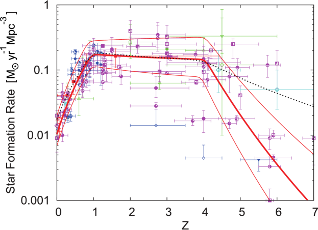
Figure 1.— [Color online] Piecewise linear star formation rate function from our fit to the subset of observed dust-corrected data. Red, blue, magenta, light blue, and green points show the observed data in IR, optical, UV, X-ray / $\gamma$-ray, and radio bands, respectively. Red lines show the SFR as function of redshift $z$ deduced from $\chi^{2}$ fitting, along with the $\pm 1\sigma$ upper and lower limits to the SFR. The reduced $\chi^{2}_{r}$ for the fit is 2.3. The black dotted line shows the SFR based upon the data set used in Yüksel et al. (2008).

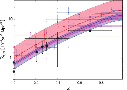
Figure 2.— [Color online] Supernova rate function $R_{SN}$ for the lower redshift interval $0\leq z\leq 1$ deduced from the SFR shown in Figure 1 via Eq. (5). This is compared with the observed supernova rate. Red thick solid line and its associated band are the best fit $R_{SN}$ function and the $\pm$ 1$\sigma$ error. Closed black circles show the measured SN rates (Li et al. (2011b), Cappellaro et al. (1999), Botticella et al. (2008), Cappellaro et al. (2005), Bazin et al. (2009), Dahlen, et al. (2004)). The blue thick line shows the best fit SN rate function from these direct supernova measurements. The blue thin lines show the upper and lower limits for a fit to the direct observations are taken from the LOSS measurement [see Leaman et al. (2011), Li et al. (2011a) and Li et al. (2011b)].

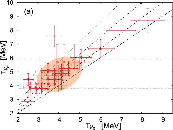
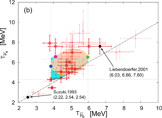
Figure 3.— [Color online] (a) The correlation between T${}_{\nu_{e}}$ and T${}_{\bar{\nu_{e}}}$. (b) The correlation between T${}_{\bar{\nu_{e}}}$ and T${}_{\nu_{x}}$. In (b) Green, red, magenta, blue, yellow and two black circles show the 7 representative points with (T${}_{\bar{\nu_{e}}}$, T${}_{\nu_{x}}$) = (6.0 MeV, 6.5MeV), (5.0 MeV, 6.0 MeV), (4.1MeV, 6.5MeV), (3.9MeV, 5.6MeV), (4.5MeV, 4.7MeV), (6.7MeV, 7.6MeV) and (2.5MeV, 2.5MeV), respectively. The Black circle at (6.7MeV, 7.6MeV) is from Liebendörfer et al. (2001), and the point at (2.5MeV, 2.5MeV) is from Suzuki (1993). These 7 pairs of T_ν are used in deriving the uncertainty in the SRN energy spectra. In both figures the orange colored ellipse indicates the 1$\sigma$ contour around the central value. The horizontal dotted lines in (a) [Vertical lines in (b)] show upper and lower limits of T${}_{\bar{\nu_{e}}}$. Straight lines show T${}_{\nu_{x}}$/T${}_{\bar{\nu_{e}}}=1/1.0,1/0.9,1/0.8,1/0.7$. The light blue area in (b) shows the allowed region of T${}_{\bar{\nu_{e}}}$-T${}_{\nu_{x}}$ pairs as discussed in the text. Red closed circles with error bars show T${}_{\bar{\nu_{e}}}$-T${}_{\nu_{x}}$ pairs derived from original numerical simulations. The error bars denote the estimated $\pm$10% change in neutrino temperatures with time as discussed in the text.

Figure 4.— Total number flux of SRN (thick line) and flux arising from various redshift bins (as labeled) as a function of $\bar{\nu_{e}}$ energy, assuming (T${}_{\bar{\nu_{e}}}$, T${}_{\nu_{x}}$) = (5.0 MeV, 6.0 MeV). Each panel presents a different oscillation case. Panel (a) is for oscillation Case I ($\bar{\nu_{e}}$ = 0.7 $\times$ $\bar{\nu_{e}}^{0}$ + 0.3 $\times$ $\nu_{x}^{0}$). Panel (b) is for oscillation Case II ($\bar{\nu_{e}}$ = ${\nu_{x}}^{0}$). Panel (c) is for no oscillations (Case III). The thin black line indicates the background noise from atmospheric neutrinos. The intersections of the SRN flux with the background sets the upper detection limit at $\sim 33-37$ MeV for the total neutrino spectrum.

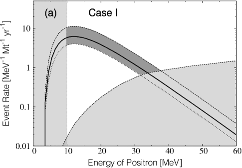
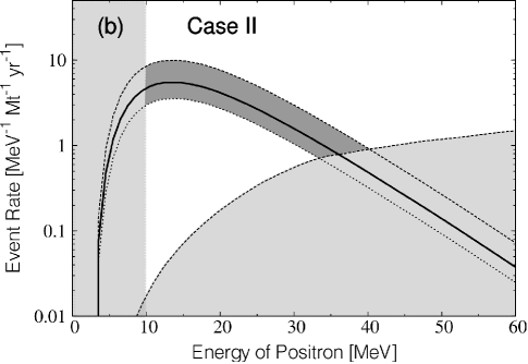
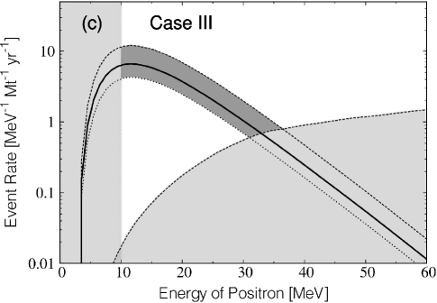
Figure 5.— Predicted $\bar{\nu_{e}}$ detection rate as a function of e⁺ energy for a 10⁶ ton class water Čerenkov detector with 1 year of run time assuming the piecewise linear SFR from the present work assuming neutrino temperatures of (T${}_{\bar{\nu_{e}}}$, T${}_{\nu_{x}}$) = (5.0 MeV, 6.0 MeV). The thick line shows the predicted SRN detection rate for the piecewise linear SFR. Thin lines show the $\pm 1\sigma$ uncertainty due to the uncertainty in the SFR fit. Panel (a) is for oscillation Case I ($\bar{\nu_{e}}$ = 0.7 $\times$ $\bar{\nu_{e}}^{0}$ + 0.3 $\times$ $\nu_{x}^{0}$). Panel (b) is for oscillation Case II ($\bar{\nu_{e}}$ = ${\nu_{x}}^{0}$), and panel (c) is for no oscillations (Case III). The shaded region in the energy range of 0 - 10 MeV indicates the region where background noise due to terrestrial nuclear reactor $\bar{\nu_{e}}$ may dominate. The shaded region that intersects the spectrum at $\sim 33$ to $37$ MeV indicates the background from atmospheric neutrinos.

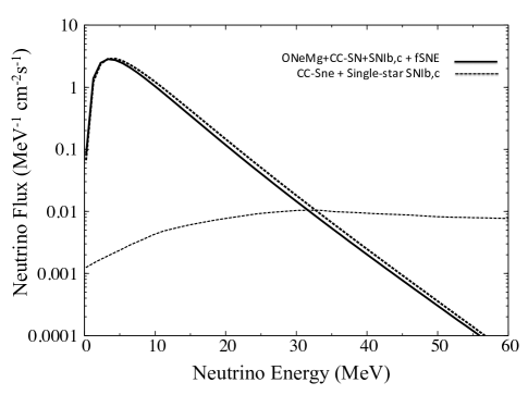
Figure 6.— Dependence of the predicted total SRN flux (upper panel) and the detection rate (lower ) on the adopted models for SNIb,c, fSNe, and ONeMg SNe in the case of a fiducial neutrino temperature of (T${}_{\bar{\nu_{e}}}$, T${}_{\nu_{x}}$) = (5.0 MeV, 6.0 MeV) and no oscillations. The solid line is for the model model with CC-SNe plus ONeMg SNe and binary SNIb,c as described in the text. The dashed line is for the single-star SNIb,c, as adopted in Horiuchi et al. (2011). The dotted line in the upper panel and the dark shaded regions in the lower panel show the neutrino backgrounds as described in Fig. 5.

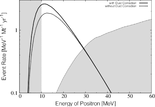
Figure 7.— Energy dependence of the SRN detection rate for two models of the SFR from Kobayashi et al. (2000). The solid line shows the detection rate based upon a model fit to the SFR data corrected for dust extinction. The dashed line is based upon a fit to the SFR data without the dust correction. Shaded regions indicate the neutrino backgrounds.

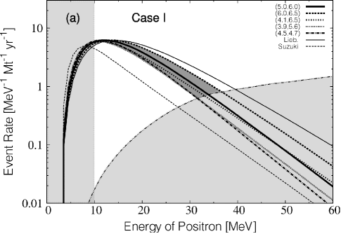
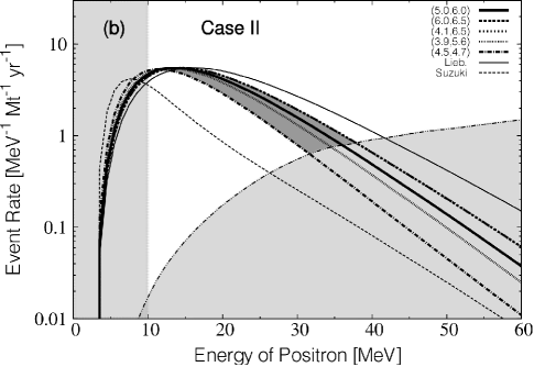
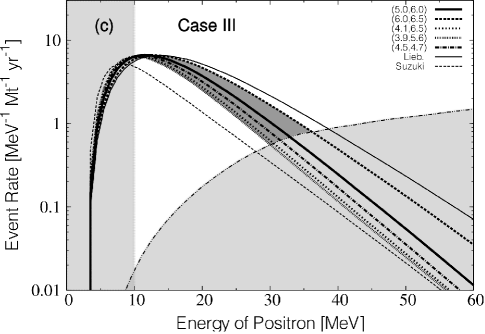
Figure 8.— $T_{\nu}$ dependence of predicted SRN detection rate from normal core collapse supernovae as a function of e⁺ energy for a 10⁶ ton class water Čerenkov detector with 1 year of run time. The three panels are for the three neutrino oscillation cases as labeled. The shaded energy range below10 MeV indicates the region where the background noise due reactor $\bar{\nu_{e}}$ may dominate. The shaded energy range that intersects the spectrum at $\sim 33$ to $37$ MeV indicates the region where the background may be dominated by noise from atmospheric neutrinos. The solid, short-dashed, long-dashed, long dash-dotted, short dash-dotted, thin line, and dotted lines as labeled represent the energy spectra for SRN detection rates assuming that (T${}_{\bar{\nu_{e}}}$, T${}_{\nu_{x}}$) = (6.7MeV, 7.6MeV), (6.0 MeV, 6.5MeV), (5.0 MeV, 6.0 MeV), (4.1MeV, 6.5MeV), (3.9MeV, 5.6MeV), (4.5MeV, 4.7MeV), (2.5MeV, 2.5MeV), respectively. Lines labeled as Lieb. (6.7MeV, 7.6MeV) and Suzuki (2.5MeV, 2.5MeV) are from Liebendörfer et al. (2001) and Suzuki (1993), respectively. The dark shaded region in each figure shows the uncertainty in the detected SRN $e^{+}$ energy spectra due to the neutrino temperature uncertainty adopted in this study.

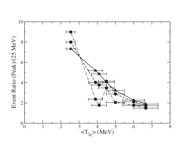
Figure 9.— Sensitivity or the ratio of events at the observed positron peak peak to events with a positron energy of 25 MeV, corresponding to the 7 fiducial SN collapse models considered here. Circles and dashed line are from Fig. 8a (oscillation Case I). Squares and dot-dashed line are from Fig. 8a (oscillation Case II). Triangles and solid line are from Fig. 8 (no oscillations Case III). This illustrates how the observed positron spectrum might be used to infer the supernova neutrino temperature. Error bars drawn indicate the adopted 10% uncertainty in model neutrino temperatures due to the variation of neutrino temperature with time during the explosion. The vertical scatter in the points indicates the uncertainty due to oscillation parameters.

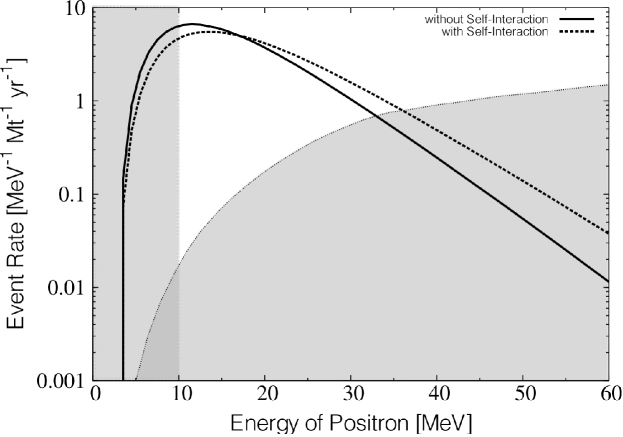
Figure 10.— Detected SRN energy spectrum for our fiducial model in cases with (dashed line) or without (solid line) of a single-angle neutrino self interaction and no neutrino oscillations. Shaded regions are the backgrounds as defined in Fig. 5.

Figure 11.— Relative contributions to the total to the total predicted SRN flux spectrum (Solid line) from CC-SNe (short dashed line), ONeMg SNe (dotted line), fSNe (long dashed line) and GRBs (dot-dashed line) for our fiducial model and three oscillation cases. The background due to atmospheric neutrinos is also indicated as a short dashed line.

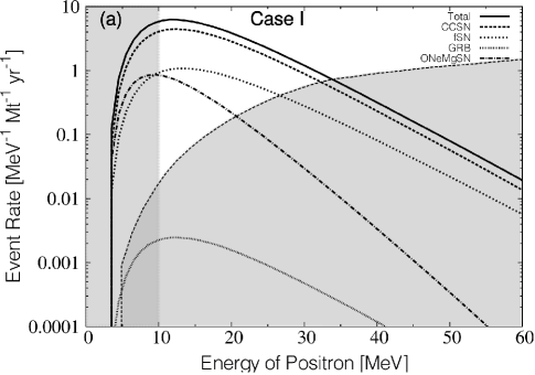
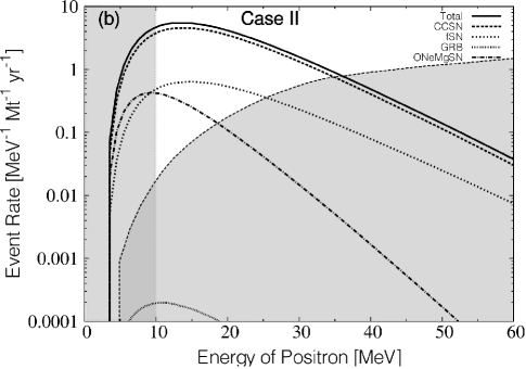
Figure 12.— Relative contributions to the total SRN detection rate (solid line) from rom CC-SNe (short dashed line), ONeMg SNe (dotted line), fSNe (long dashed line) and GRBs (dot-dashed line) for our fiducial model and three oscillation cases. Shaded regions are backgrounds as defined in Figure 5.

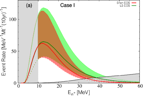
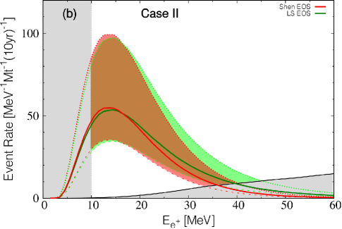
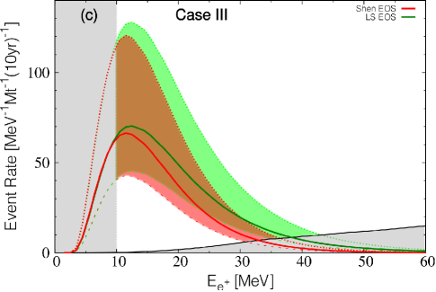
Figure 13.— Predicted $e^{+}$ energy spectra and uncertainty of the total SRN detections for the fiducial model and massive SFR deduced here. Uncertainty is based upon the SFR and the detector statistics. Each panel corresponds to the case of: (a) non-adiabatic oscillations (Case I); (b) adiabatic oscillations (Case II); and (c) no oscillations (Case III). Red, line and shaded region is for fSNe models based upon the stiff RMF EoS of Shen et al. (1998). The green line and shaded region is for fSNe based upon the soft EoS of Lattimer & Swesty (1991). Grey regions denote the backgrounds as defined in Figure 5.

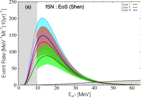
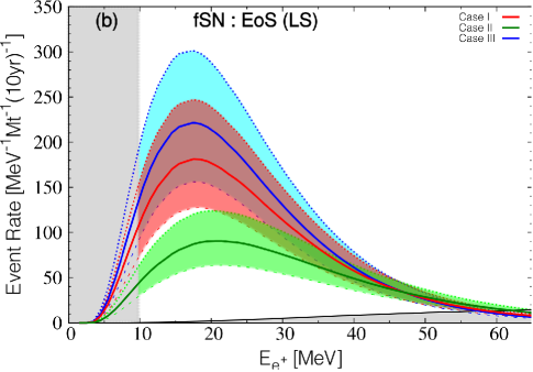
Figure 14.— Predicted $e^{+}$ energy spectra and uncertainty of the SRN detection rate as a function of $e^{+}$ energy for a $10^{6}$ ton water Čerenkov detector with 10 years of run time. Shown are cases in which failed fSNe account for a factor of two difference between supernova rate deduced from the massive SFR and the observed supernova rate. Red, green, and blue lines shows the SRN detection rate in the case of non-adiabatic (Case I), adiabatic (Case II), or no neutrino oscillations (Case III), respectively. Light red, light green, and light blue areas show the uncertainty in the SRN detection rate in each oscillation case due to the SFR of Horiuchi et al. (2011) and the detector statistics. The vertical light grey areas denote the backgrounds. Each figure presents: (a) the case that all the missing SNe are fSN modeled with the stiff EoS of Shen et al. (1998); (b) the case that all the missing SNe are fSN modeled with the soft EoS of Lattimer & Swesty (1991).

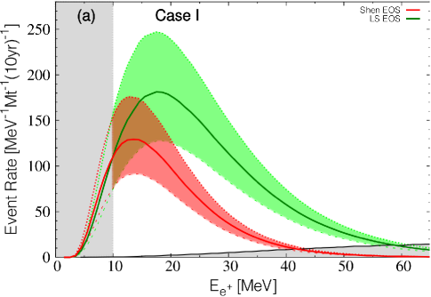
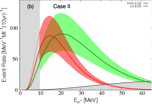
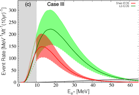
Figure 15.— Same as Fig.12 but in this case the three different cases of neutrino oscillations shown in separate panels. Red, green, and blue lines show the SRN detection rate in the case that all of the missing SNe are fSN with the stiff RMF EoS of Shen et al. (1998), and the case that all the missing SNe are fSN modeled with the soft EoS of Lattimer & Swesty (1991). Light red, light green, and light blue areas show the uncertainty in the SRN detection rate based upon the SFR of Horiuchi et al. (2011) and the detector statistics. Each figure represents the case of: (a) non-adiabatic oscillations (Case I); (b) adiabatic oscillations (Case II); and (c) no oscillations (Case III).

Table 1Coefficients for the piecewise linear star formation rate

	$\dot{\rho}_{0}$	$\alpha$	$\beta$	$\gamma$	$B$	$C$
	(M⊙Mpc${}^{-3}y^{-1}$)
Best Fit	0.0104	4.22	-0.20	-11.30	2.70$\times 10^{6}$	6.37
Upper limit	0.0200	4.22	0.14	-9.0	1.25$\times 10^{-8}$	6.87
Lower limit	0.0069	4.22	-0.42	-13.60	1.6$\times 10^{3}$	5.90

Table 2Results of numerical simulations in previous work.

model	time(s)	T${}_{\nu_{e}}$	T${}_{\bar{\nu_{e}}}$	T${}_{\nu_{x}}$	$\eta_{\nu_{e}}$	$\eta_{\bar{\nu_{e}}}$	$\eta_{\nu_{x}}$	$<e>$ or $\surd<e^{2}>$
		(MeV)	(MeV)	(MeV)
Mayle et al. (1987)	-	3.80	7.60	6.98	0.33	0.3	0.33	-
Bruenn (1987)	-	3.17	3.80	7.93	-	-	-	-
Janka & Hillebrandt (1989)	-	2.54	4.44	5.08	$\sim$0	$\sim$0	$\sim$0	$<e>$
Myra & Burrows (1990)	time table	3.49	4.12	7.60	-	-	-	$<e>$
Suzuki (1990)	1.0	3.02	4.13	4.76	-	-	-	-
Suzuki (1990)	20.0	2.54	3.17	2.85	-	-	-	-
Suzuki (1991)	1.0	2.63	4.13	4.76	-	-	-	-
Suzuki (1991)	15.0	2.54	2.85	3.02	-	-	-	-
Suzuki (1993)	1.0	2.85	3.80	4.13	-	-	-	-
Suzuki (1993)	15.0	2.22	2.54	2.54	-	-	-	-
Totani et al. (1998)	0.3	3.80	4.76	6.03	-	-	-	-
Totani et al. (1998)	10.0	3.40	6.35	7.93	-	-	-	-
Liebendörfer et al. (2001)	-	6.03	6.66	7.60	-	-	-	$\surd<e^{2}>$
Mezzacappa et al. (2001)	-	5.08	6.03	7.60	-	-	-	-
Ando & Sato (2003)	mean	3.49	5.08	6.98	-	-	-	$<e>$
Ando & Sato (2003)	fulltime	3.49	4.44	5.71	-	-	-	$<e>$
Buras et al. (2003)	0	4.48	5.24	5.33	-	-	-	$\surd<e^{2}>$
Buras et al. (2003)	0.15	4.13	5.08	7.30	-	-	-	$\surd<e^{2}>$
Beacom & Vagins (2004)	-	3.20	5.00	6.00	-	-	-	-
Gil-Botella & Rubbia (2003) 1	-	3.49	5.08	7.94	-	-	-	-
Gil-Botella & Rubbia (2003) 2	-	4.13	5.08	7.30	-	-	-	-
Gil-Botella & Rubbia (2003) 3	-	4.13	5.08	5.59	-	-	-	-
Gil-Botella & Rubbia (2003) 4	-	4.13	5.08	5.59	-	-	-	-
Gil-Botella & Rubbia (2003) 5	-	4.13	5.08	5.59	-	-	-	-

Table 3Results of numerical simulations in previous works(2).

model	time(s)	T${}_{\nu_{e}}$	T${}_{\bar{\nu_{e}}}$	T${}_{\nu_{x}}$	$\eta_{\nu_{e}}$	$\eta_{\bar{\nu_{e}}}$	$\eta_{\nu_{x}}$	$<e>$ or $\surd<e^{2}>$
		(MeV)	(MeV)	(MeV)
Accretion Phase model 1	-	4.13	4.76	5.71	2.8	3.4	1.1	$<e>$
-Keil et al. (2003)	-	3.80	4.44	4.44	1.4	2.7	0.6-1.6	-
Accretion Phase model 2	-	4.13	5.07	5.40	1.7	3.0	0.8	-
-Keil et al. (2003)	-	4.13	4.76	5.07	2.1	3.2	0.8	-
Lunardini & Smirnov (2003)	-	2.22-5.58	4.44-6.98	4.88-11.17	0.0-3.0	0.0-3.0	0.0-2.0	-
Rosswog & Liebendörfer (2003) C	-	4.20	5.50	8.90	-	-	-	-
Rosswog & Liebendörfer (2003) D	-	4.10	5.00	6.60	-	-	-	-
Rosswog & Liebendörfer (2003) E	-	5.00	5.70	9.10	-	-	-	-
Selvi & Vissani (2003)	-	4.00	5.00	7.50	-	-	-	-
Vogel (2003)	-	3.50	5.10	8.00	-	-	-	-
Dighe et al (2004) G	-	3.81	4.79	5.71	-	-	-	-
Dighe et al (2004) L	-	3.81	4.79	7.62	-	-	-	-
Gil-Botella & Rubbia (2004)	-	2.22-5.71	4.44-6.98	4.76-11.11	0.0	0.0	0.0	-
Tomàs (2004) L	-	3.81	4.76	7.62	-	-	-	-
Tomàs (2004) G1	-	3.81	4.76	5.71	-	-	-	-
Tomàs (2004) G2	-	3.81	4.76	4.76	-	-	-	-
Yoshida et al. (2004)	-	3.20	5.00	6.00	-	-	-	-
Balantekin & Yüksel (2005)	-	4.13	4.76	5.08	0.0	0.0	0.0	-
Barger (2005)	-	2.22-6.29	4.44-6.98	4.44-11.17	-	-	-	-
Athar (2005)	-	3.17-3.49	4.76-5.08	7.30-7.94	-	-	-	-
Sumiyoshi et al. (2005) SH	1.0	7.00	7.80	7.10	-	-	-	$\surd<e^{2}>$
Sumiyoshi et al. (2005) LS	1.0	8.30	8.70	8.40	-	-	-	$\surd<e^{2}>$
Beacom & Strigari (2006)	-	4.00	5.00	8.00	0.0	0.0	0.0	-
Bekman et al. (2006)	-	3.50	5.00	8.00	0.0	0.0	0.0	-

Table 4Results of numerical simulations in previous works(3).

model	time(s)	T${}_{\nu_{e}}$	T${}_{\bar{\nu_{e}}}$	T${}_{\nu_{x}}$	$\eta_{\nu_{e}}$	$\eta_{\bar{\nu_{e}}}$	$\eta_{\nu_{x}}$	$<e>$ or $\surd<e^{2}>$
		(MeV)	(MeV)	(MeV)
Choubey & Kar (2006)	-	3.50	5.00	8.00	0.0-3.0	0.0-3.0	0.0-2.0	-
Olive & Sandick (2006)	-	4.22	4.86	6.35	0.0	0.0	0.0	-
Suzuki et al. (2006)	-	3.17	4.76	4.76-7.94	0.0	0.0	0.0	-
Yoshida et al. (2006)a	-	3.20	5.00	6.00	-	-	-	-
Yoshida et al. (2006)b	-	3.20	5.00	6.66	-	-	-	-
Agafonova (2007)	-	3.17-3.81	3.49-5.40	4.76-7.62	0.0	0.0	0.0	-
Baker et al. (2007)	-	4.13	4.89	4.98	-	-	-	-
Chakraborty et al. (2008) LL	-	3.81	4.76	7.62	-	-	-	-
Chakraborty et al. (2008) G1	-	3.81	4.76	5.71	-	-	-	-
Chakraborty et al. (2008) G2	-	3.81	4.76	4.76	-	-	-	-
Dasgupta et al. (2008)	-	3.17	4.76	6.35	-	-	-	-
Dighe et al (2008) Liv	-	3.81	4.76	7.62	-	-	-	-
Dighe et al (2008) Gar	-	3.81	4.76	5.81	-	-	-	-
Kneller et al. (2008)	-	3.81	4.76	5.71	-	-	-	-
Yoshida et al. (2008) 1	-	3.20	5.00	6.00	-	-	-	-
Yoshida et al. (2008) 2	-	4.00	4.00	6.00	-	-	-	-
Yoshida et al. (2008) LT	-	3.20	5.00	6.50	-	-	-	-
Yoshida et al. (2008) ST	-	3.20	4.20	5.00	-	-	-	-
Dasgupta (2009)	-	4.76	5.71	5.71	-	-	-	-
Fischer et al. (2012)	1.0	2.9	3.8	4.3	-	-	-	$<e>$
Roberts (2012)	-	2.6	3.9	3.5	-	-	-	$<e>$

Table 5Percentage contribution to the total neutrino flux and detected events for various redshift bins.

$z_{min}$	$z_{max}$	% events	% flux
0.	5.	100.	100.
0.0	0.1	5.9	3.7
0.1	0.2	6.6	4.6
0.2	0.3	7.2	5.3
0.3	0.4	7.6	6.0
0.4	0.5	7.8	6.7
0.5	0.6	8.0	7.2
0.6	0.7	7.9	7.6
0.7	0.8	7.8	7.9
0.8	0.9	7.6	8.0
0.9	1.0	6.9	7.7
1.0	1.1	5.7	6.6
1.1	1.2	4.5	5.4
1.2	1.3	3.5	4.4
1.3	1.4	2.7	3.5
1.4	1.5	2.1	2.9
1.5	1.6	1.7	2.3
1.6	1.7	1.3	1.9
1.7	1.8	1.0	1.5
1.8	1.9	0.8	1.2
1.9	2.0	0.7	1.0
2.0	2.1	0.5	0.8
2.1	2.2	0.4	0.7
2.2	2.3	0.3	0.6
2.3	2.4	0.3	0.5
2.4	2.5	0.2	0.4
2.5	5.0	1.0	1.6

Table 6Percentage contributions to the total neutrino flux and detected events for various redshift bins using the SFR models of Kobayashi et al. (2000) with dust extinction corrected data (DC) or data without dust correction (no DC).

$z_{min}$	$z_{max}$	DC flux	no DC flux	DC Events	no DC Event
0.0	0.1	6.7	8.9	9.6	12.0
0.1	0.2	6.4	8.4	6.7	10.7
0.2	0.3	5.9	7.8	7.6	9.4
0.3	0.4	5.5	7.2	6.7	8.3
0.4	0.5	5.3	7.0	6.1	7.5
0.5	0.6	5.2	6.8	5.7	7.0
0.6	0.7	5.1	6.7	5.4	6.6
0.7	0.8	5.1	6.7	5.1	6.3
0.8	0.9	5.5	6.9	5.3	6.3
0.9	1.0	6.6	6.3	6.1	5.4
1.0	1.1	7.1	5.5	6.3	4.6
1.1	1.2	6.5	4.4	5.5	3.6
1.2	1.3	5.5	3.6	4.6	2.8
1.3	1.4	4.6	2.9	3.7	2.2
1.4	1.5	3.8	2.3	3.0	1.7
1.5	1.6	3.1	1.8	2.3	1.3
1.6	1.7	2.5	1.4	1.8	1.0
1.7	1.8	2.0	1.1	1.4	0.8
1.8	1.9	1.9	0.9	1.1	0.6
1.9	2.0	1.3	0.7	0.9	0.5
2.0	2.1	1.0	0.6	0.7	0.4
2.1	2.2	0.8	0.4	0.5	0.3
2.2	2.3	0.6	0.3	0.4	0.2
2.3	2.4	0.5	0.3	0.3	0.2
2.4	2.5	0.4	0.2	0.3	0.1
2.5	5.0	1.5	0.7	0.9	0.4

Table 7SRN detected events for 10 yr running in a 10⁶ ton water Čerenkov detector for various redshift bins and oscillation cases I, II, III.

$(T_{\bar{\nu}_{e}},T_{\nu_{x}}$)	total	z=0-1	1-2	2-3	3-4	4-5
Oscillation Case I
(6.7,7.6)	1092	744	299	41	8.3	0.8
(5.0,6.0)	814	587	202	22	3.0	0.3
(6.0,6.5)	963	674	252	31	4.9	0.5
(4.1,6.5)	716	522	173	18	2.6	0.3
(3.9,5.6)	649	483	150	14	1.9	0.2
(4.5,4.7)	682	508	156	15	1.8	0.1
(2.5,2.5)	314	245	63	5.8	0.8	0.1
Oscillation Case II
(6.7,7.6)	1102	728	316	47	9.2	1.1
(5.0,6.0)	851	592	226	28	4.4	0.4
(6.0,6.5)	934	638	255	34	5.8	0.6
(4.1,6.5)	934	638	255	34	5.8	0.6
(3.9,5.6)	782	552	203	24	3.5	0.3
(4.5,4.7)	622	457	148	14.6	1.9	0.2
(2.5,2.5)	2281	178	44	4.6	0.71	0.1
Oscillation Case III
(6.7,7.6)	10891	752	292	38	6.4	0.7
(5.0,6.0)	800	587	191	19	2.4	0.2
(6.0,6.5)	975	689	251	30	4.5	0.4
(4.1,6.5)	633	481	138	12	1.3	0.1
(3.9,5.6)	595	456	127	11	1.2	0.1
(4.5,4.7)	708	523	162	15	1.7	0.1
(2.5,2.5)	350	273	70	6.4	0.8	0.1

Table 8Neutrino temperature dependence of the total SRN detection events for a 10⁶ton water Čerenkov detector with a 10 yr run time for oscillation cases I, II, III. .

($T_{\bar{\nu}_{e}},T_{\nu_{x}}$)	$N(I)$	$N(II)$	$N(III)$
( 6.7 , 7.6 )	836	826	842
( 6.0 , 6.5 )	745	709	761
( 5.0 , 6.0 )	638	650	636
( 4.1 , 6.5 )	567	709	515
( 3.9 , 5.6 )	519	601	487
( 4.5 , 4.7 )	545	487	570
( 2.5 , 2.5 )	268	191	300

Table 9Parameters for the neutrino sources considered in this work.

detail	ONeMg SN	SNII	SNIb,c	fSN(SH EoS)	fSN(LS EoS)	GRB
mass(M☉)	(8 - 10)	8 - 25(10-25)1	8-40(10-40)1	25 - 125 (99.96$\%$)	25 - 125 (99.96$\%$)	25 - 125 (0.04$\%$)
Remnant	Neutron Star	Neutron Star	Neutron Star	Black Hole	Black Hole	Black Hole
Phenomenon	Dim Supernova	Supernova	Supernova	Failed Supernova	Failed Supernova	Gamma-Ray Burst
T${}_{\nu_{e}}$(MeV)	3.0	3.2	3.2	5.5	7.9	3.2
T${}_{\bar{\nu_{e}}}$(MeV)	3.6	5.0	5.0	5.6	8.0	5.3
T${}_{\nu_{x}}$(MeV)	3.6	6.0	6.0	6.5	11.3	4.4
E${}_{\nu_{e}}^{total}$(erg)	3.3$\times 10^{52}$	5.0$\times 10^{52}$	5.0$\times 10^{52}$	5.5$\times 10^{52}$	8.4$\times 10^{52}$	1.7$\times 10^{53}$
E${}_{\bar{\nu_{e}}}^{total}$(erg)	2.7$\times 10^{52}$	5.0$\times 10^{52}$	5.0$\times 10^{52}$	4.7$\times 10^{52}$	7.5$\times 10^{52}$	3.2$\times 10^{53}$
E${}_{\nu_{x}}^{total}$(erg)	1.1$\times 10^{52}$	5.0$\times 10^{52}$	5.0$\times 10^{52}$	2.3$\times 10^{52}$	2.7$\times 10^{52}$	1.9$\times 10^{52}$
$\triangle$ t	few $s$	few $s$	few $s$	- 0.5$s$	- 0.5$s$	- 10$s$

Table 10SRN detection rate contributions from core collapse SNe, ONeMg SNe, failed SNe, and GRBs in a 10⁶t water Čerenkov detector with 10 yr run time.

	total	z = 0-1	1-2	2-3	3-4	4-5
Case I
Total	814	586	201	21.8	3.01	0.275
SNe	593	425	149	16.2	2.21	0.200
ONeMg SNe	62.7	51.1	10.9	0.612	0.0406	0.0019
Failed SNe	158	110	42	5.00	0.749	0.073
GRB	0.327	0.235	0.0815	0.0087	0.0012	0.00010
Case II
Total	851	592	226	28.0	4.40	0.45
SNe	713	494	191	23.6	3.69	0.37
ONeMg SNe	31.2	25.5	5.40	0.30	0.02	0.00035
Failed SNe	107	72	30.2	4.07	0.69	0.08
GRB	0.0190	0.0152	0.0035	0.00028	0.000027	0.000002
Case III (no osc.)
Total	637	487	134	13.1	1.61	0.182
SNe	412	315	87.3	8.41	0.992	0.107
ONeMg SNe	62.7	52.9	9.26	0.505	0.0324	0.0019
failed SNe	161	119	37.80	4.21	0.584	0.0738
GRB	0.020	0.016	0.004	0.0004	0.0003	0.000002

References

- Abe et al. (2003) Abe,.K., et al., 2011, (Hyper-Kamiokande working group) unpublished Letter of Intent, arXiv:1109.3262 [hep-ex]
- Agafonova (2007) Agafonova, N., Yu., et al., 2007, ApPh, 27, 254
- An et al. (2012) An, F. P. et al. (Daya Bay Collaboration), 2012, Phys. Rev. Lett., 108, 171803
- Ando & Sato (2003) Ando, S. & Sato, K., 2003, Phys. Rev. D, 67, 023004
- Ando (2004) Ando, S., 2004, ApJ, 607, 20
- Arnett et al. (1989) Arnett, D., et al. 1989, ARA&A, 27, 629
- Arnouts et al. (2005) Arnouts, S., et al., 2005, ApJ, 619, L43
- Athar (2005) Athar, M., S., et al., 2005, Phys. Rev. C, 71, 045501
- Baker et al. (2007) Baker, J., et al., 2007, Phys. Rev. D, 76, 063004